The Acoustic Detection of Ultra High Energy Neutrinos
Jonathan David Perkin
Department of Physics and Astronomy
The University of Sheffield

Thesis submitted for the Degree of Doctor of Philosophy in the
University of Sheffield
$\cdot$ April 2007 $\cdot$

Abstract

Attempts have been made to parameterise the thermoacoustic emission of particle cascades induced by EeV neutrinos interacting in the sea. Understanding the characteristic radiation from such an event allows us to predict the pressure pulse observed by underwater acoustic sensors distributed in kilometre scale arrays. We find that detectors encompassing thousands of cubic kilometres are required, with a minimum of 100 hydrophones per kilometre cubed, in order to observe the flux of neutrinos predicted by the attenuation of ultra high energy cosmic rays on cosmic microwave background photons. The pressure threshold of such an array must be in the range $5\to 10$ mPa and the said detector will have to operate for five years or more. Additionally a qualitative analysis of the first acoustic data recorded by the Rona hydrophone array off the north-west coast of Scotland is reported.

For
Mum and Dad

Contents

1. 1 Introduction
   1. 1.1 A Brief History of the Neutrino
   2. 1.2 Neutrinos in the Standard Model and Beyond
   3. 1.3 Sources of Ultra High Energy Neutrinos
      1. 1.3.1 Bottom-Up neutrino production
      2. 1.3.2 Top-Down neutrino production
   4. 1.4 Observations of Trans-GZK CRs and Limits on the UHECR Flux
   5. 1.5 Summary
2. 2 Neutrino Detection Methods
   1. 2.1 Introduction
   2. 2.2 Deep Inelastic Scattering
   3. 2.3 Optical Čerenkov Neutrino Telescopes
      1. 2.3.1 AMANDA
      2. 2.3.2 ANTARES
      3. 2.3.3 Lake Baikal
      4. 2.3.4 NESTOR
      5. 2.3.5 Kilometre-Cubed optical Čerenkov neutrino telescopes
      6. 2.3.6 Limits on the neutrino flux from optical Čerenkov neutrino telescopes
   4. 2.4 Radio Čerenkov Detectors
      1. 2.4.1 ANITA
      2. 2.4.2 FORTE
      3. 2.4.3 GLUE
      4. 2.4.4 LOFAR/LOPES
      5. 2.4.5 RICE
      6. 2.4.6 SALSA
      7. 2.4.7 Limits on the neutrino flux from radio Čerenkov neutrino telescopes
   5. 2.5 Acoustic Detection of UHE Neutrinos
      1. 2.5.1 The LPM effect
      2. 2.5.2 Formation of the acoustic signal
      3. 2.5.3 Laboratory based measurements of thermoacoustic emission
      4. 2.5.4 Experimental results from SAUND
   6. 2.6 Practical Motivation for the Acoustic Technique
      1. 2.6.1 “Back of the envelope” comparison of effective volumes for an optical neutrino telescope and an acoustic telescope with 1000 sensors
   7. 2.7 Summary
3. 3 Simulating Neutrino Interactions
   1. 3.1 Introduction
   2. 3.2 Neutrino Event Generation
   3. 3.3 Simulating Neutrino Induced Particle Cascades
      1. 3.3.1 Physics processes
      2. 3.3.2 Particle production thresholds
   4. 3.4 Formation of the Acoustic Signal
   5. 3.5 Summary
4. 4 Simulating the Propagation of the Acoustic Signal
   1. 4.1 Introduction
   2. 4.2 Attenuation of the Acoustic Signal
      1. 4.2.1 Geometric attenuation
      2. 4.2.2 Attenuation by the medium
      3. 4.2.3 Angular spread
   3. 4.3 Refraction
   4. 4.4 Ambient Noise, Filtering and Thresholds
   5. 4.5 Summary
5. 5 Large Scale Detector Simulation
   1. 5.1 Introduction
   2. 5.2 The Sensitivity Estimation Procedure
   3. 5.3 Neutrino Spectra and Geometries Used
   4. 5.4 Event Reconstruction
      1. 5.4.1 Vertex location with linear rays
      2. 5.4.2 Vertex location with curvilinear rays
   5. 5.5 The Effective Volume
   6. 5.6 Optimal Hydrophone Density for Reconstruction in the Presence of Refraction
   7. 5.7 The Effect of Uncertainty in Hydrophone Locations
   8. 5.8 Reconstruction of the Neutrino Energy
   9. 5.9 The Sensitivity Calculation and Predicted Results
   10. 5.10 Summary
6. 6 First Data from Rona Underwater Acoustic Range
   1. 6.1 Introduction
   2. 6.2 Data Acquisition
      1. 6.2.1 Recording the hydrophone signals
      2. 6.2.2 Reducing the data
      3. 6.2.3 Rona calibration tones
   3. 6.3 A Novel Analysis of the Reduced Data
      1. 6.3.1 Event discrimination
      2. 6.3.2 Categorisation of events
      3. 6.3.3 Time dependence of events
      4. 6.3.4 Recurring event types
   4. 6.4 Summary
7. 7 Discussion and Outlook
   1. 7.1 The Motivation for Neutrino Astronomy
   2. 7.2 The Current Scale of Development
   3. 7.3 Simulation of Acoustic Arrays
      1. 7.3.1 Neutrino interactions
      2. 7.3.2 Formation and propagation of the signal
      3. 7.3.3 Noise and filtering
      4. 7.3.4 The large scale detector simulation
   4. 7.4 Predictions for Future Work
8. A Empirical Data
   1. A.1 Neutrino-Nucleon Cross Section
   2. A.2 Knudsen Noise Curves
9. B Comparison of Hadronic Showers from Geant4 and CORSIKA
10. C Formalism of Ray Tracing Algorithm
11. D Neutrino Source Data
12. E Recurring Event Types at Rona

List of Figures

1. 1.1 The cosmic ray spectrum
2. 1.2 Cosmic acceleration
3. 1.3 GRB Cannonball
4. 1.4 GZK neutrino fluxes
5. 1.5 Domain structures in a ferromagnet
6. 1.6 The measured UHECR flux
7. 2.1 Deep inelastic scattering
8. 2.2 Čerenkov light cone
9. 2.3 Antarctic Muon And Neutrino Detector Array
10. 2.4 AMANDA sky plot
11. 2.5 Limits on the neutrino flux from optical telescopes
12. 2.6 UHE cascades in the lunar regolith
13. 2.7 Limits on the neutrino flux from radio telescopes
14. 2.8 Schematic of the energy deposition
15. The 1979 Brookhaven-Harvard experiments
16. 2.12 SAUND schematic
17. 2.13 Limits on the neutrino flux from SAUND
18. 2.14 Simple cubic lattice
19. 2.15 Energy windows for neutrino detection techniques
20. 3.1 Propagation of neutrinos through the Earth’s crust
21. 3.2 Neutrino range in Earth’s crust
22. 3.3 Three flavour Bjorken-$y$ distribution
23. 3.4 Comparison of neutrino event generators
24. 3.5 Average energy deposited by one hundred $100$ TeV proton showers
25. 3.6 Effect of physics lists on radial shower shape
26. 3.7 Effect of physics lists on longitudinal shower shape
27. 3.8 Acoustic pressure signal from a $100$ TeV proton induced shower
28. 3.9 Peak pulse pressure vs. shower energy
29. 4.1 Sound attenuation coefficient for seawater
30. 4.2 Attenuation by seawater
31. 4.3 Angular spreading of acoustic pulses
32. 4.4 Oceanic depths of constant sound gradient
33. 4.5 Refraction geometry
34. 4.6 Computing the ray start angle
35. 4.7 Ray trace from detector simulation
36. 4.8 Ray trace for ANTARES SVP
37. 4.9 A natural limit on source distance imposed by refraction
38. 4.10 Matched filter performance
39. 5.1 Neutrino source locations
40. 5.2 Coordinate systems
41. 5.3 Unsmeared $x$-coordinate resolution
42. 5.4 Finding the pointing vector
43. 5.5 Pointing reconstruction
44. 5.6 Pointing resolution without refraction
45. 5.7 Schematic of refracted thermoacoustic energy deposition
46. 5.8 Reduced-mean $x$-coordinate resolution
47. 5.9 Reduced v.s. unreduced mean $x$-coordinate resolution
48. 5.10 Minimised $x$-coordinate resolution
49. 5.11 Range of detectable events
50. 5.12 Effective volume as a function of hydrophone density
51. 5.13 Vertexing performance v.s. hydrophone density
52. 5.14 Pointing reconstruction v.s. hydrophone density
53. 5.15 Energy reconstruction: $\chi^{2}$ minimisation
54. 5.16 Reconstructed energy v.s. actual energy
55. 5.17 Energy resolution
56. 5.18 Sensitivity of simulated arrays
57. 6.1 $10$ kHz oscillating signal at Rona
58. 6.2 Rona triggers
59. 6.3 $10$ kHz oscillating signal on $6$ channels
60. 6.4 A high frequency signal
61. Transient events
62. 6.7 Temporal distribution of Rona events
63. 6.8 A short-lived impulsive event
64. 6.9 A low frequency oscillating event
65. 6.10 A $10$ kHz sinusoidally oscillating event
66. 6.11 A high frequency event
67. 6.12 A ‘ringing’ event
68. 6.13 A ‘bipolar’ event
69. A.1 Neutrino-Nucleon cross section
70. A.2 Knudsen Noise Curves
71. B.1 Geant4 and CORSIKA longitudinal energy deposition at $10^{4}$ eV
72. B.2 Geant4 and CORSIKA longitudinal energy deposition at $10^{5}$ eV
73. B.3 Geant4 and CORSIKA radial energy deposition at $10^{4}$ eV
74. B.4 Geant4 and CORSIKA radial energy deposition at $10^{5}$ eV
75. C.1 Refraction Geometry
76. E.1 A short-lived impulsive event
77. E.2 A low frequency oscillating event
78. E.3 A $10$ kHz sinusoidally oscillating event
79. E.4 A high frequency event
80. E.5 A ‘ringing’ event
81. E.6 A ‘bipolar’ event

List of Tables

1. 1.1 The leptons
2. 1.2 Core topologies for different defects
3. 2.1 Attenuation lengths for different techniques
4. 5.1 Shower time errors
5. 5.2 Minimised vertex performance
6. 5.3 The effect of $0.1$ m uncertainty on hydrophone locations
7. 6.1 Peakiness of Rona events
8. 6.2 Frequency composition of Rona events
9. 6.3 Recurrence of events at Rona
10. 6.4 Level of coincidence at Rona

Chapter 1 Introduction

Chapters 1 and 2 of this thesis summarise the history of our understanding of neutrinos and the methods by which they can be detected. Chapters 3, 4 and 5 discuss the potential performance of hypothetical large scale neutrino detectors. Chapter 6 reports an analysis of data from an underwater acoustic sensor array situated in the north west of Scotland in the United Kingdom. Finally, in Chapter 7 a discussion summarising this work and making predictions for future work is given.

1.1 A Brief History of the Neutrino

Neutrinos are the second most abundant known particles in the Universe after cosmological photons. They are produced copiously, for example, by stellar bodies, like the Sun, throughout their considerable lifetimes and during their spectacular deaths. There are, on average, three hundred million neutrinos per cubic metre of space, billions penetrate our bodies unnoticed every second. However, neutrinos remain poorly understood.

It is because neutrino interactions are mediated only by the weak nuclear and gravitational forces that they acquire their mystery. However, it is this very same reason that makes them attractive to the astronomer. Whereas charged particles are deflected by magnetic fields, photons are absorbed by inter-stellar matter and softened by radiation fields, and more massive particles fall deeper into gravitational wells; the neutrino traverses the Cosmos retaining its energy and directionality until it eventually undergoes a collision far away from its place of origin. Should such a collision occur on Earth it could yield information from parts of the Universe no other form of light or matter can reach.

Whilst detection of neutrinos has been achieved, there has been no direct measurement of their rest mass. In fact, evidence of neutrino mass has only recently come to light. The development of our understanding of neutrinos, pertaining to neutrino astronomy, is illustrated in the following time-line (adapted from [1]):

• Charles Drummond Ellis and James Chadwick et al firmly establish that the beta decay spectrum is continuous [2],[3], contrary to the predictions of a two body decay: $n\to p+e^{-}$.

• Wolfgang Pauli postulates the existence of a third, neutral particle present in beta decay to explain the observed $\beta$ energy spectrum [4]: $n\to p+e^{-}+\nu_{neutral}$.

• Enrico Fermi incorporates Pauli’s neutral particle into beta decay theory and bestows it the name “neutrino” (little neutral one) [5]. The continuous beta decay energy spectrum is explained.

• Fred Reines and Clyde Cowan detect neutrinos from the Hanford Nuclear Reactor using a delayed-coincidence technique on the reaction: $\overline{\nu}+p\to n+\beta^{+}$ [6]. Neutrinos were registered through observation of the photons emitted simultaneously by capture of the neutron $n$ and annihilation of the positron $\beta^{+}$.

• Bruno Pontecorvo makes the first hypothesis of neutrino oscillation, in this instance between neutrino and anti-neutrino states [7].

• Ray Davis Jr measures the Solar Neutrino Flux in the Homestake Mine. He observes a deficit in the number of interactions compared to predictions by John Bahcall’s Standard Solar Model. This deficit becomes known as the “Solar Neutrino Problem” [8].

• The tau lepton is discovered at SLAC and through analysis of its decay it is concluded that the tau is accompanied by its own unique flavour of neutrino, the tau neutrino [9].

• The Kamiokande experiment confirms the solar neutrino deficit. Then, along with IMB, the first measurements of neutrinos from a supernova (SN) are made [10], [11]. Neutrino Astronomy is born.

• LEP constrains the number of light neutrino species to three: electron, muon and tau [12].

• Super-Kamiokande reports on the flavour oscillation of atmospheric neutrinos, direct evidence for three different neutrino mass states [13].

• Twenty four years after the tau lepton is discovered, DONUT reports on the first direct observation of the tau neutrino [14].

• The Sudbury Neutrino Observatory detects both neutral and charged current interactions from solar neutrinos, evidence is mounting in support of oscillations as a solution to the Solar Neutrino Problem [15].

• KAMLAND confirms neutrino oscillations consistent with the observed solar neutrino deficit, this time with reactor neutrinos [16].

• AMANDA produces the most detailed neutrino sky-map ever, with no evidence (yet) of point sources [17].

• The cubic kilometre extension of AMANDA, codenamed IceCube is under construction at the South pole [18]. ANTARES nears completion on the Mediterranean sea bed [19]. Neutrino Astronomy is in full flight.

1.2 Neutrinos in the Standard Model and Beyond

Neutrinos belong to a family of particles called “Leptons” (from the Greek word leptos meaning small or fine). Leptons exist in three flavours and each forms a couplet of one charged and one neutral particle as illustrated in Table 1.1:

$e^{-}$	$\mu^{-}$	$\tau^{-}$	$q=e$
$\nu_{e}$	$\nu_{\mu}$	$\nu_{\tau}$	$q=0$

Table 1.1: The leptons.

The Standard Model (SM) of particle physics predicts that neutrinos are massless, spin half, fermions interacting only via the weak nuclear force. This imposes the condition that all neutrinos are left-handed (and all anti-neutrinos are right-handed), since, in the massless limit it is impossible to boost to a frame of reference where a neutrino with left handed helicity (projection of spin in the direction of momentum) has a right handed chirality (the sign of the helicity).

The SM has been constructed from Quantum Field Theories (QFTs) that explain the unification of the electromagnetic and weak nuclear forces into the electro-weak force via Quantum Electro Dynamics (QED) and the interpretation of strong nuclear interactions via Quantum Chromo Dynamics (QCD). Within these QFTs there is no gravitational component, so, although the SM describes to great precision a wealth of experimental data, it remains for this reason, amongst many others, an incomplete theory. Furthermore, as has already been intimated, it does not contain a neutrino mass term.

Although it was not realised at the time, the Solar Neutrino Problem was evidence for neutrino flavour oscillations. A free neutrino propagating through space exists in a superposition of fundamental mass eigenstates $\nu_{1}$, $\nu_{2}$ and $\nu_{3}$ the mixing of which gives rise to the three neutrino flavours $\nu_{e}$, $\nu_{\mu}$ and $\nu_{\tau}$. The neutrino flavours are in fact manifestations of weak nuclear eigenstates. This can be illustrated in the form of a matrix equation:

$$\left(\begin{array}[]{l}\nu_{e}\\ \nu_{\mu}\\ \nu_{\tau}\\ \end{array}\right)=\left(\begin{array}[]{lll}U_{e1}&U_{e2}&U_{e3}\\ U_{\mu 1}&U_{\mu 2}&U_{\mu 3}\\ U_{\tau 1}&U_{\tau 2}&U_{\tau 3}\\ \end{array}\right)\left(\begin{array}[]{c}\nu_{1}\\ \nu_{2}\\ \nu_{3}\\ \end{array}\right)$$ (1.1)

where $U$ is the $3\times 3$ unitary Maki-Nakagawa-Sakata (MNS) matrix [20]. This is analogous to mixing in the quark sector as described by the Cabibbo Kobayashi Maskawa (CKM) matrix [21]. The unitary matrix $U$ can be decomposed into three rotations:

$$U=\left(\begin{array}[]{ccc}1&0&0\\ 0&c_{23}&s_{23}\\ 0&-s_{23}&c_{23}\\ \end{array}\right)\left(\begin{array}[]{ccc}c_{13}&0&e^{-i\delta_{CP}}s_{13}\\ 0&1&0\\ -e^{i\delta_{CP}}s_{13}&0&c_{13}\\ \end{array}\right)\left(\begin{array}[]{ccc}c_{12}&s_{12}&0\\ -s_{12}&c_{12}&0\\ 0&0&1\\ \end{array}\right)$$ (1.2)

where the abbreviations $s_{ij}\equiv sin\theta_{ij}$ and $c_{ij}\equiv cos\theta_{ij}$ are employed. This decomposition allows us to describe three-flavour neutrino mixing in terms of six parameters: three mixing angles $\theta_{12}$, $\theta_{23}$ and $\theta_{13}$; a complex, CP violating phase $\delta_{CP}$; and, two mass-squared differences $\Delta m^{2}_{12}=m^{2}_{2}-m^{2}_{1}$ and $\Delta m^{2}_{23}=m^{2}_{3}-m^{2}_{2}$. The sign of $\Delta m^{2}_{23}$ determines the neutrino mass hierarchy; it is said to be “normal” if $\Delta m^{2}_{23}>0$, or, “inverted” if $\Delta m^{2}_{23}<0$. Experiments in neutrino oscillation look for an appearance or disappearance in one of the neutrino flavours as a result of mixing. $\theta_{23}$ and $\Delta m_{23}$ are traditionally known as the “atmospheric” mixing parameters describing $\nu_{\mu}\to\nu_{\tau}$ oscillations; and, $\theta_{12}$ and $\Delta m_{12}$ are the “solar” mixing parameters, concerned with $\nu_{e}\to\nu_{\mu}$ flavour oscillations. In each case a deficit (or disappearance) of the expected flux of the first flavour is seen as a result of oscillation into the second kind.

Neutrino oscillations have implications for the neutrino astronomer. The flux of neutrinos from cosmic accelerators is predominantly the result of pion decays into muons and neutrinos, essentially producing no $\nu_{\tau}$, i.e. $\phi_{\nu_{e}}:\phi_{\nu_{\mu}}:\phi_{\nu_{\tau}}=1:2:0$. However, since the length of propagation from source to observer is very much greater than the baseline for oscillation, it is expected that by the time extra-terrestrial neutrinos arrive at the Earth they will be evenly mixed: $\phi_{\nu_{e}}:\phi_{\nu_{\mu}}:\phi_{\nu_{\tau}}=1:1:1$.

1.3 Sources of Ultra High Energy Neutrinos

Many theoretical models have been proposed that predict fluxes of Ultra High Energy Neutrinos (UHE$\nu$s). A recent, short review is presented in [22]; for the interested reader an exhaustive review is given by [23]. Mechanisms in which Cosmic Rays (CRs) are accelerated to UHE ($E>1$ EeV, where $1$ EeV$=10^{18}$ eV) are described as “Bottom-Up” scenarios. The subsequent weak decay of such CRs through $pp$ collisions and interaction with ambient, or intergalactic, radiation fields produces an associated flux of UHE neutrinos. So-called “Top-Down” neutrino production can occur through various exotic mechanisms such as: the weak decay of GUT scale particles produced during early cosmological epochs; annihilation of superheavy Dark Matter (DM) particles; and effects due to the existence of Quantum Gravity. Furthermore they can be a signature of “beyond the standard model” processes such as violation of Lorentz Invariance and enhancements to the neutrino-nucleon cross section. A brief discussion of Bottom-Up and Top-Down processes follows.

1.3.1 Bottom-Up neutrino production

Bottom-Up neutrino production relies exclusively on the acceleration of charged particles of cosmological origin as an injector to the neutrino flux. For instance, once a CR proton has been accelerated to UHE, it can disintegrate into pions following a collision with another proton; this subsequently produces neutrinos when the pions decay.

The cosmic ray spectrum

The high energy ($E>1$ GeV) CR spectrum, as plotted in Figure 1.1, extends a further twelve decades of energy throughout which the intensity reduces by $33$ orders of magnitude. Some $94$ years since Victor Hess first discovered CRs their origin is still widely debated. The CR flux below $E>1$ GeV is dominated by the Solar Wind: coronal ejecta that are readily captured in the Earth’s magnetic field, giving rise to the aurora phenomenon. The interstellar low energy CR flux is thus very difficult to determine. Despite being of great interest, low energy CRs will not be discussed further.

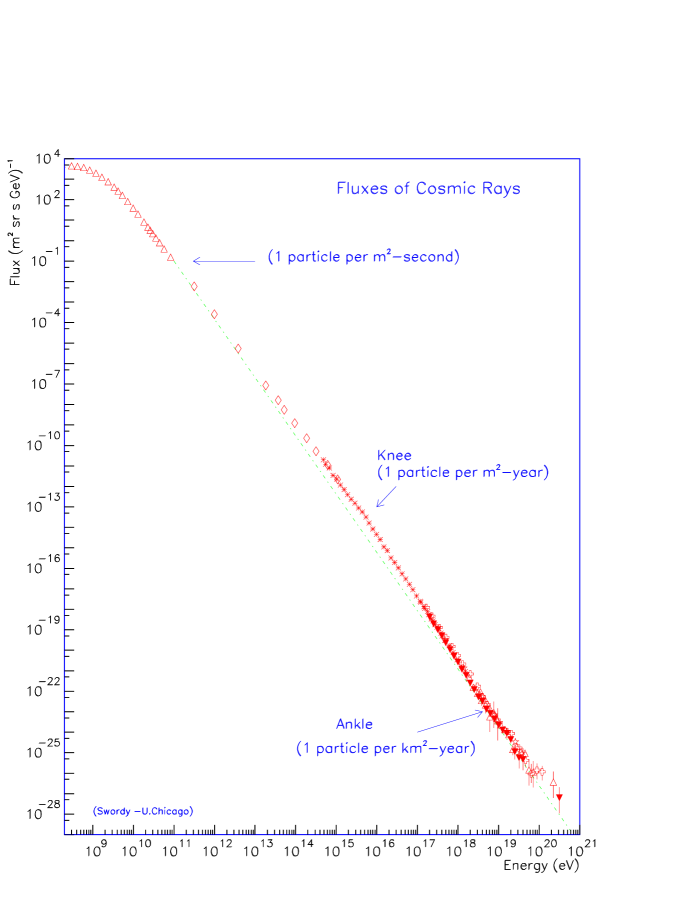
Figure 1.1: Above $1$ GeV the cosmic ray spectrum (from [24]) is well described by a broken $E^{-\gamma}$ power law, with $\gamma=2.7$ and two distinguishing features, caused by a change in spectral index $\gamma$, at $10^{14}$ eV, labelled ‘knee’ and at $10^{18}$ eV, labelled ‘ankle’.

Traditionally the CR spectrum has been well described in terms of two main features, namely the “knee” and the “ankle”. Both are due to a deviation from the underlying power law distribution, due to a change in spectral index (see caption of Figure 1.1). The causes of each of them remain a controversial topic. The origin of the “knee”, seen as a bump in the spectrum at a CR energy around $10^{14}$ eV, remains an unsolved problem, to which some of the proposed answers include: a change in CR composition, interactions with a Galactic DM halo, collisions with massive neutrinos, and different acceleration mechanisms to produce the CRs. The change in flux at the ankle has traditionally been interpreted as a transition from Galactic to extragalactic CRs. More recently it has been suggested that the contribution of extragalactic CRs is of importance at lower energies, not far above $10^{17}$ eV [25]. Furthermore, extra detail in the spectrum may yet be resolved as more experimental data is acquired, not least a potential second knee and perhaps a toe.

The concept behind Bottom-Up UHECR and UHE$\nu$ generation is illustrated in Figure 1.2. The Waxman-Bahcall (WB) [26] bound on the neutrino flux assumes that all neutrinos result from CRs accelerated at optically thin (i.e transparent to CRs) sites. Subsequently these CRs undergo $pp$ and $p\gamma$ collisions after they leave the acceleration site. This bound is however speculative, as it assumes that all the energy of the proton is transferred to the resultant pion following a collision; in reality the pions, and consequently the neutrinos, will have lower energy. The WB bound can be exceeded by non-accelerator neutrino sources, or if they exist, accelerator sites that are opaque to CRs such that they do not appear in the observed CR flux.

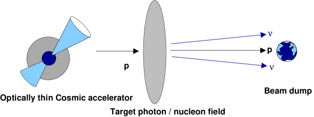
Figure 1.2: Protons are accelerated to UHEs at acceleration sites across the Universe. Matter and radiation fields provide target material for $pp$ and $p\gamma$ collisions, producing an associated flux of UHE neutrinos.

Shock acceleration mechanisms

“Fermi” acceleration is one of the driving forces that underpins the generation of UHECRs. The process of Fermi acceleration involves a transference of the bulk kinetic energy of a plasma to the individual ions it contains. Ions are accelerated, over long periods of time, by shock fronts - regions of compression in the plasma at the interface of two areas at different pressures. Successive head on collisions with a shock front tend to increase the kinetic energy of an ion. This mechanism is sufficient to produce the observed power law spectrum of CRs. However, one must add some non-linearity, to describe the shock reaction to ion acceleration, and thus ensure the energy spectrum does not diverge. Acceleration occurs in the relativistic outflows that surround a powerful central engine, such as a super-massive Black Hole (BH) in an Active Galactic Nucleus (AGN). Local inhomogeneities in the turbulent magnetic field structures confine ions initiating a random walk. Whilst the ion velocities are changed by magnetic confinement, the kinetic energy is not. It is possible for an ion to receive multiple kicks from a single shock if its random walk overtakes the compression front many times, eventually leading to relativistic ion velocities.

A second method of acceleration, resulting from bulk magnetised plasma inhomogeneities has been motivated by observational evidence. It is known as “collisionless shock acceleration” because ions are accelerated by the electromagnetic field of the plasma rather than by particle-particle collisions. The details of magnetic fields throughout the Cosmos remain elusive and continue to be actively studied; there is mounting evidence that collisionless shock acceleration can describe the observed CR spectrum from multiple sources. [27].

Acceleration sites throughout the Cosmos

Traditionally Supernova Remnants (SNR) have been regarded as the primary Galactic acceleration sites for high energy CRs below the knee. The observation of radio, optical and X-ray emission accompanying the emission of charged particles from such regions has long provided evidence for electron acceleration up to multi-GeV energies. Under the assumption that protons and other ions will be accelerated in places where electron acceleration occurs, the difficult task of determining the leptonic and hadronic components of such regions is underway. In particular, X-ray images from the CHANDRA satellite support CR acceleration in the forward blast wave of a SNR, a thin shell in the outer shock [28]. This has been determined from various details such as the shape and form of the emission, and the observed spectra.

If SNRs are typical accelerators for Galactic CRs then Active Galactic Nuclei are the traditional sites of CR acceleration beyond the Milky Way. The standard model of an AGN is comprised of a central super-massive BH surrounded by a dusty torus of matter which forms an accretion disk in the equatorial plane. Axial relativistic jets of charged particles are emitted as accreted matter falls on to the central BH. It is in the AGN jets that shock acceleration takes place. In the case where the relativistic outflow is directed towards the Earth an AGN is detected distinctly as a gamma ray source and is classified as a Blazar.

An alternative candidate accelerator is the Gamma Ray Burst (GRB). GRBs are the most energetic events observed in the Universe. There are two breeds of GRB: short, typically lasting less than two seconds; and long, typically lasting tens of seconds. The luminosity of a GRB is of the order $10^{45}$ J and can exceed that of the combined luminosity of all the stars contained within its host galaxy. The sudden gamma ray emission is now thought to be the result of a rapid mass accretion onto a compact body, resulting from events such as core collapse supernovae in stars of a few solar masses, or binary mergers . The result of such an event is a relativistic outflow of charged particles that penetrates the surrounding medium, sweeping up and accelerating ions, however the mechanism by which these relativistic outflows are produced remains a hot topic.

A novel, cannonball (CB) model, of GRBs has been formulated from the hypothesis that following a core collapse SN into a neutron star or BH, an accretion disk is formed around the compact body [29]. A CB is emitted when a large chunk of the accretion matter falls abruptly onto the compact object. The GRB photons are produced as the CB falls through the ambient radiation of the host SN and photons are Compton scattered up to GRB frequencies, see Figure 1.3. Again CR acceleration occurs in the shock fronts of the relativistic outflow.

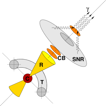
Figure 1.3: Schematic of the GRB cannonball model: A “plasmoid” is seeded by an abrupt collapse of matter from the torus (T) onto the compact body (C). A cannonball (CB) is ejected along the relativistic outflow (R), and, as it passes through the remnants of the parent supernova (SNR) photons ($\gamma$) Compton Scatter up to GRB energies.

The GZK mechanism

A golden channel for neutrino production exists through pion photo-production from UHECR protons. This takes place via excitation of the $\Delta^{+}$ resonance resulting from interaction with $2.7$ K Cosmic Microwave Background (CMB) photons, as formulated in Equation 1.3:

$$p+\gamma_{\textrm{CMB}}\to\Delta^{+}\to n+\pi^{+}$$ (1.3)

where

$$n\phantom{x} \to p+e^{-}+\overline{\nu_{e}}$$

$$\pi^{+} \to \mu^{+}+\nu_{\mu}$$

$$\mu^{+} \to e^{+}+\nu_{e}+\overline{\nu_{\mu}}$$

This reaction was postulated first by Kenneth Greisen [30] and later, independently by Zatsepin and Kuzmin [31], and has been dubbed the GZK mechanism. The threshold energy for pion production by CR protons on photons of energy $7\times 10^{-4}$ eV (the mean energy of black-body radiation at $2.7$ K) is $\approx 5\times 10^{19}$ eV. Some pion photo-production occurs below this threshold because of the high-frequency tail of the black-body photon spectrum. The consequence of this process is to limit the source distance of UHECR protons to within $\approx 50$ MPc, (within the extent of our local group of galaxies) the typical attenuation length in the CMB photon field at this energy. The flux of GZK neutrinos appears in Figure 2.13. It is highly desirable that a neutrino telescope be sensitive to the flux of cosmogenic neutrinos produced via the GZK mechanism, since this represents what is essentially a guaranteed signal, and a smoking gun for EeV scale CR proton acceleration. Predictions of the flux of GZK neutrinos must satisfy constraints on the diffuse gamma ray background due to the process: $\Delta^{+}\to p+\pi^{0}$, where $\pi^{0}\to\gamma\gamma$, which competes with the process in Equation 1.3. Such limits are presently set by the Energetic Gamma Ray Experiment Telescope (EGRET), a satellite borne detector sensitive to gamma rays in the energy range $20$ MeV to $30$ GeV. Furthermore, they are dependent on an assumed initial proton flux. An example of different GZK neutrino fluxes is presented in Figure 1.4. Also noteworthy is the photonic analogue of this mechanism, whereby CR photons are attenuated by the cosmic infrared, microwave and radio backgrounds.

Figure 1.4: Cosmogenic neutrino fluxes (from [32]) as a function of energy. The thick solid line (max) is for an initial proton flux $\propto 1/E$, assuming that the EGRET flux is entirely due to pion-photoproduction. The thin solid line ($0.2$) shows the neutrino flux when the associated photons contribute only up to $20\%$ of the EGRET flux. The dashed line indicates an initial proton flux $\propto 1/E^{2}$. The experimental points represent the UHECR flux measured by AGASA (crosses) and HiRes (asterisks) - see Section 1.4 for further discussion.

1.3.2 Top-Down neutrino production

The apparent lack of suitable candidate sites for particle acceleration up to UHE, within our neighbourhood, has motivated the investigation of possible non-accelerator sources. Here, UHE neutrinos constitute some of the decay products of arbitrary, super-massive, $X$ particles. $X$ particle production can occur through a number of mechanisms, including the decay of topological defects (a spontaneous break in symmetry during a transition in phase); metastable super heavy (i.e. $m>10^{21}$ eV) relic particles left over from the Big Bang; or very massive Dark Matter (DM) particles. Furthermore, extensions beyond SM physics, such as extra-dimensional regimes, can provide scenarios for the production of UHE neutrinos.

$X$ particles from topological defects

Topological Defects (TD) in states of matter occur as a result of symmetry breaking phase transitions. Terrestrial examples include vortex lines in superfluid helium, magnetic flux tubes in type II semiconductors and disinclination lines in liquid crystals. One usually envisages the formation of TDs as a result of thermal phase transitions. For instance, a ferromagnet acquires domain structures as it is cooled through its Curie point and a symmetry is spontaneously broken (see Figure 1.5). An extensive review of TD models, including their generation and topologies, is presented in Bhattacharjee and Sigl’s 2000 Paper “Origin and Propagation of Extremely High Energy Cosmic Rays” [33]. After the Big Bang it is natural to assume that there may have been some temperature through which the Universe cooled and underwent a similar process, acquiring domain structures [34].

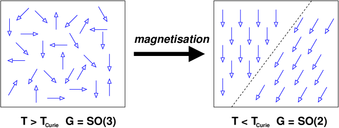
Figure 1.5: As a ferromagnet is cooled through its Curie temperature it forms domain regions of aligned magnetic field separated by Bloch walls (dotted line). Spontaneous symmetry breaking occurs as one requires the introduction of a new degree of freedom: net magnetisation to describe the state of the system. Hence there is a transition from the SO(3) to SO(2) group symmetry.

This method of formation, however, appears to contradict the inflationary paradigm, which is to dilute the concentration of unwanted TDs by introducing an exponential expansion of the Universe through an inflationary phase. It has, though, been realised that TD formation can take place after inflation by way of non-thermal phase transitions. Such models have been created that allow for abundances of quasi-stable TDs that can exist at present in the Universe [35]. In summary, even if the Universe undergoes a period of inflation during an early cosmological epoch, TD formation can form at a later time, due to non-thermal phase transitions, thus remaining in concordance with the inflationary paradigm.

Topological Defects can be described in terms of their Higgs field, the underlying quantum field predicted by theory, with which ordinary matter interacts in order to acquire mass (an analogous process is that by which massive objects moving through fluids experience drag). Generally, if $\eta$ is the vacuum expectation value (VEV) of a Higgs field in a broken symmetry phase, then an associated TD has core size $\sim\eta^{-1}$. At the centre of a core the Higgs field vanishes, the topologies of core centres are given in Table 1.2.

Core Topology	Topological Defect
point	monopole
line	cosmic string
surface	domain wall

Table 1.2: Core topologies for different defects.

Far outside of the core, symmetry is broken and the Higgs fields are in their proper ground states. Hence the ‘defect’ is a core region of unbroken symmetry (“false vacuum”) surrounded by broken symmetry regions (“true vacuum”). The energy densities of the gauge and Higgs fields within the defect are higher than outside and they are stable due to a ‘winding’ of the Higgs fields around the cores. Energy is therefore trapped inside the cores and it is in this way that the TDs acquire mass. In general the mass of the TD, $m_{TD}$, is proportional to $T_{c}$ where $T_{c}$ is the critical temperature of the defect forming phase transition. For a monopole $m_{TD}\sim T_{c}$, for a cosmic string the mass per unit length $m_{TD}\sim T_{c}^{2}$ and for a domain wall the mass per unit area $m_{TD}\sim T_{c}^{3}$. For generic symmetry breaking potentials of the Higgs field, $T_{c}\sim\eta$ [33]. Topological Defects can be envisaged as trapped quanta of massive gauge and Higgs fields of the underlying spontaneously broken gauge theory. Sometimes there are quanta of fermion fields trapped in the defect cores because of their coupling to the massive gauge and Higgs fields, this combination of fields effectively constitutes a massive object contained within the defect - this is the $X$ particle.

Metastable superheavy relic particles as $X$ particles

Metastable Superheavy Relic Particles (MSRPs) are an expected bi-product of inflation. In certain models MSRPs can exist in the present with sufficient abundance as to act as a source of non-thermal, superheavy dark matter [33]. A well cited description of CR production from relics of inflation is given in [36]. One has to overcome the problem of producing a particle that has a lifetime that is both finite and long enough for it to survive to the present cosmological epoch. This paves the way for the introduction of exotic physics such as quantum gravity and instantons. Any model put forward must adhere to present day limits set by experiment. It suffices to say that until there are higher statistics for the most energetic events, there will exist an abundance of theories proposing MSRP progenitors to the UHECR and UHE neutrino fluxes.

1.4 Observations of Trans-GZK CRs and Limits on the UHECR Flux

As stated in Section 1.3.1 the threshold energy for the GZK mechanism is $\approx 5\times 10^{19}$ eV. To date, AGASA, AUGER and HiRes have all reported the existence of particles above this threshold. The UHECR flux they have measured is shown in Figure 1.6. The appearance of CRs above the GZK threshold suggests that the origin of such CRs is within our local group of galaxies despite there being no known sources, or more specifically acceleration regions contained therein, that can produce CRs at such energies. As the number of events recorded at these energies slowly increases it should become apparent if they are a component of the diffuse CR background or they originate from point sources.

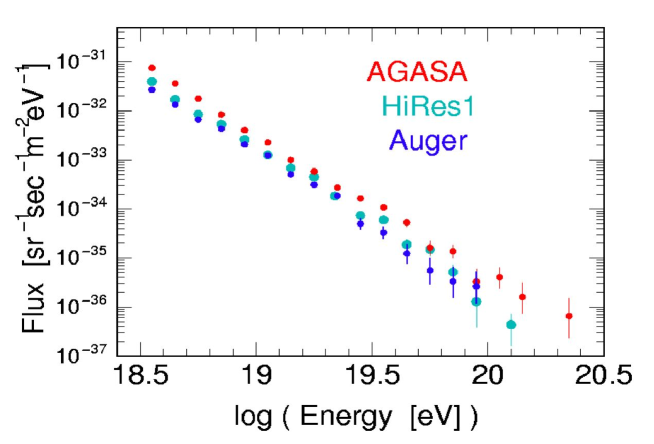
Figure 1.6: The flux of UHE Cosmic Rays (from [37]) as measured by AGASA, AUGER and HiRes. The highest energy AUGER event ($>140$ EeV) does not appear in this plot because the core of the shower fell outside the surface detector and as such it did not pass all quality cuts for flux calculations.

1.5 Summary

It has been shown in this chapter how neutrinos come to reach the Earth from various cosmological origins, most of which are not fully understood. The discovery of neutrino mass and subsequently flavour oscillations means that although one expects muon type neutrinos to outnumber electron type neutrinos by two to one, with no tau neutrino component; in fact, by the time of their arrival at Earth they are evenly mixed into equal fractions.

The flux of UHE neutrinos in which the Earth bathes is intimately linked to the acceleration and subsequent decay of UHECRs. Wherever proton acceleration has occurred, one can expect to encounter the production of neutrinos with comparable vigour. The electromagnetic and hadronic components of cosmological accelerator outflow are retarded by inter galactic matter and radiation. This presents a limit on how far we can observe them through the cosmic molasses. Neutrinos however can reach us from the furthest depths of the Universe.

The UHE neutrino flux may not rely exclusively on particle acceleration. The lack of suitable acceleration sites within our vicinity has motivated the idea that the highest energy CR events that have been observed resulted from the decay of very massive entities known only as “$X$-particles”

Chapter 2 Neutrino Detection Methods

2.1 Introduction

The detection medium for Ray Davis Jr’s pioneering Homestake experiment was a large tank of tetrachloroethene [8]. This chemical, essentially a cleaning fluid, is sensitive to neutrino capture through the reaction $\nu_{solar}+{{}_{17}\mathrm{Cl}^{37}}\to e^{-}+{{}_{18}\mathrm{Ar}^{37}}$. Neutrinos are emitted by the Sun through the conversion of hydrogen to helium and in the decay of Be⁷, B⁹, N¹³ and O¹⁵. Amazingly it was by measuring the number of individual Argon atoms present after flushing out the detector that it was possible to quantify the neutrino flux of solar neutrinos through the apparatus.

Today, there are numerous experiments across the world either under construction or in operation, dedicated to the detection of astrophysical neutrinos. The principal method by which they are registered is through Čerenkov emission. This can be at optical wavelengths via their muon daughters, or at radio frequencies via the Askaryan Effect [38]. Large, natural bodies of transparent dielectric media such as Mediterranean Sea water, Antarctic ice, subterranean salt domes and even the lunar regolith can serve as natural neutrino calorimeters.

2.2 Deep Inelastic Scattering

Figure 2.1 illustrates how high energy neutrinos $l$, interact with a target nucleon $N$, by deep inelastic scattering (DIS) on its constituent quarks. The basic interaction is given by Equation 2.1:

$$l+N\to l^{\prime}+X$$ (2.1)

where $N$ is a nucleon, $l^{\prime}$ is the outgoing lepton and $X$ is one or more excited hadrons. Interactions can be neutral current (NC), as mediated by the weak-neutral $Z$ boson, or charged current (CC) as mediated by the weak-charged $W^{\pm}$ bosons. The contributions of these two components to the total neutrino-nucleon cross section are illustrated in Figure A.1 in Appendix A.1.

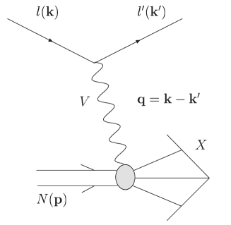
Figure 2.1: Deep inelastic scattering. $l$ is the incoming neutrino, $l^{\prime}$ the outgoing lepton; $V$ is the vector boson ($Z$ or $W^{\pm}$) and $N$ is the target nucleon. $X$ is the arbitrary excited hadronic final state. $k$, $k^{\prime}$ and $p$ are the 4-momenta of the incoming neutrino $l$, the outgoing lepton $l^{\prime}$ and the nucleon $N$ respectively.

The square momentum transfer of the interaction, also known as hardness, is defined as $Q^{2}=-q^{2}=-(\mathbf{k}-\mathbf{k^{\prime}})^{2}$. Two dimensionless scaling variables can be used to describe the kinematics of DIS, each of which represents a physical characteristic of the event. Firstly the Bjorken-x variable, defined as:

$$x=\frac{Q^{2}}{2(\mathbf{p}\cdot\mathbf{q})}$$ (2.2)

which is the fraction of the nucleon momentum carried by the participating (valence or sea, depending on $E_{\nu}$) quark. Second is the Bjorken-y variable, defined as:

$$y=\frac{\mathbf{p}\cdot\mathbf{q}}{\mathbf{p}\cdot\mathbf{k}}$$ (2.3)

which is the fraction of the lepton energy transferred to the hadronic system. In the case of a neutrino DIS then this is the fraction of the neutrino energy that goes into the hadronic cascade, the behaviour of which will be discussed further in Chapter 3.

Calorimetric registration of a neutrino DIS can result through the development of the hadronic cascade and, following CC interactions, through propagation of the charged lepton. Electrons induce an electromagnetic shower that develops collinearly to the hadronic shower, whereas muons, having a longer interaction length travel through the detector for several metres before decaying. In the case of CC tau neutrino interactions a characteristic “double bang” signal can be observed: first a hadronic cascade is initiated by the DIS which is closely followed by a displaced secondary cascade induced by the decay of the tau lepton.

Particle cascades tend to excite atoms in a calorimeter via excitation and ionisation, furthermore there is Čerenkov emission which can be observed in the visible or radio frequency band. This is explained in detail for each case below.

2.3 Optical Čerenkov Neutrino Telescopes

Optical neutrino telescopes are optimally sensitive to the weak interaction of $\nu_{\mu}$ neutrinos into muons via the process $\nu_{\mu}+N\to\mu^{-}+X$. The energy of the neutrino is shared between the resultant muon, $\mu$, and the hadronic cascade, $X$, with the muon taking between a half and three quarters of the total neutrino energy; it then continues along a path that is effectively collinear ($<0.5$ ^∘ separation for $E_{\nu}>1$ TeV) to the bearing of the incident neutrino. The charge of the traversing muon causes the surrounding medium to become polarised. Subsequent depolarisation of the medium results in the emission of Čerenkov photons along the relativistic charged particle track. Interference between photons can occur if the wavefronts overlap, which is only possible if the muon travels faster than light does in the detection medium. Hence the net polarisation of the medium is assymetric. Wavelets interfere constructively to produce the Čerenkov wavefront if $\beta(=v/c)>1/n$, where $v$ is the muon speed and $n$ is the refractive index of the medium. The range of the muon in water extends from $\sim 5$ m at $1$ GeV to $\sim 7$ km at $10$ TeV[21].

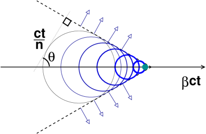
Figure 2.2: Schematic representation of Čerenkov light emission.

The number of Čerenkov photons produced, $N$, within a wavelength interval $d\lambda$ and unit distance $dx$ is given by [21]:

$$\frac{d^{2}N}{dxd\lambda}=\frac{2\pi\alpha}{\lambda^{2}}\times(1-\frac{1}{\beta^{2}n^{2}})$$ (2.4)

The wavefront formed by coherent emission of Čerenkov photons forms a cone of radiation with opening angle dependent on the velocity of the emitting particle, given by Equation 2.5. Thus if one can reconstruct the angular aperture of a Čerenkov light cone, it can be used to infer the velocity of the transient particle. One must then assume a rest mass in order to resolve the particle momentum and hence it’s energy.

$$\cos\theta=\frac{1}{\beta n}$$ (2.5)

Detection of those photons emitted is facilitated by photomultiplier tubes (PMTs), devices that convert optical quanta into charge quanta (conceptually the inverse of a light bulb). PMTs tend to be optimally sensitive at wavelengths around $450$ nm and one has to be mindful to choose a detector medium in which the scattering and absorption of such light is kept to a minimum.

Traditionally, a neutrino “telescope” views the Cosmos using the Earth as a filter to those muons produced in CR induced air showers high in the atmosphere. Hence a neutrino telescope built in the northern hemisphere, looking downward through the centre of the Earth, will see a view of the southern sky, and vice versa. Muon neutrino interactions can occur in the transparent medium surrounding the instrumentation or in the Earth’s crust below, so long as the muon has sufficient collision length to allow it to propagate through the detector, preserving the directionality of its parent neutrino. The performance of an optical neutrino telescope is limited at low energies by the short length of the muon tracks and at high energies by the opacity of the Earth. Since the neutrino-nucleon cross section increases with energy, as one looks for neutrinos with greater energy the Earth ceases to act merely as a filter and instead becomes impenetrable.

A summary of existing projects and proposed extensions follows, including, at the end of this section, the current limits on the neutrino flux as set by optical neutrino telescopes.

2.3.1 AMANDA

Undoubtedly the most advanced optical neutrino telescope to date is the Antarctic Muon And Neutrino Detector Array (AMANDA)[39]. The most recent second-phase AMANDA-II [40] is an array of $667$ downward pointing PMTs, occupying a cylinder of one kilometre height and $200$ m diameter, located $1.5$ km deep under the $3$ km thick, southern polar ice cap. Construction of AMANDA-II was completed during the austral summer of 1999-2000 following the initial phases of the shallow ice array AMANDA-A in 1993/94, AMANDA-B4 ($80$ PMTs on $4$ strings) in 1995/96 and AMANDA-B10 (an additional $216$ PMTs on $6$ strings) in 1997/98 as illustrated in Figure 2.3. Deployment of detector strings is made possible by drilling the ice with heated jets of $75$ ^∘C water. Operating at a speed of $1$ cm s^-1, it takes approximately three and a half days to bore a $50\to 60$ cm diameter hole to a depth of $2$ km. After a bore hole is formed, the strings are dropped into place and the ice re-freezes over a period of about $35$ hours.

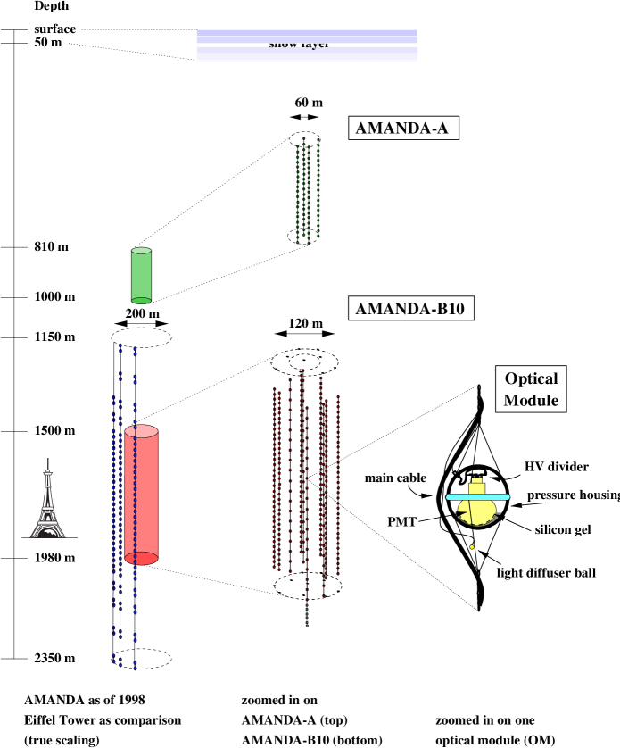
Figure 2.3: Schematic of AMANDA phases A $(1993/94)$ and B-10 $(1997/98)$ including graphic of an AMANDA optical module (OM) containing PMT. From [39].

AMANDA has been in operation for over $5$ years in its latest, phase-II, configuration collecting between $7$ and $10$ neutrinos per diem [18]. A background rate of $\sim 80$ Hz is present due to downward going muons from atmospheric CR interactions and must be rejected through angular cuts and event reconstruction. Point source searches have been performed using the first four years of AMANDA neutrino data and limits on the neutrino flux have been estimated using $800$ days of data [39]. Further analysis is currently underway. The most significant point source excess, located in the direction of the Crab Nebula, has a confidence level of only $3.4\sigma$ [18]. A view of the sky as viewed through AMANDA is plotted in Figure 2.4. Clearly there is a case for a kilometre cubed extension to AMANDA if decisive identification of point sources is to be made. IceCube [18] will incorporate the existing AMANDA-II instrumentation and extend to a total of $4800$ active PMTs and furthermore include IceTop - an array of surface based scintillator detectors for the purpose of calibration, background rejection and CR studies.

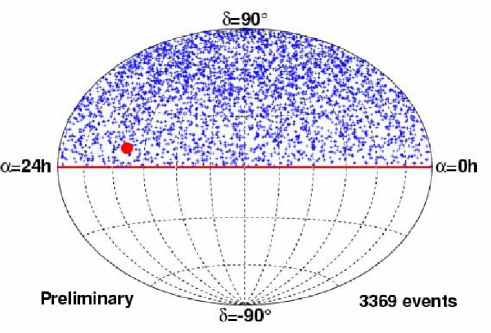
Figure 2.4: The sky as viewed through the AMANDA neutrino telescope (from [18]) with the coordinates of the crab $\alpha=19.2h$, $\delta=9.2$ ^∘ highlighted by the $\bullet$ marker.

2.3.2 ANTARES

The ANTARES (Astronomy with a Neutrino Telescope and Abyssal Environmental RESearch) neutrino telescope is currently under construction in the Mediterranean Sea, off the coast of southern France [19] . It consists of twelve $480$ m long strings each bearing $75$ ten inch Hammamatsu PMTs arranged three per storey, each enclosed in a pressure resistant glass sphere (PMT$+$sphere$=$optical module (OM)), with a declination angle of $45$ ^∘. This declination helps limit the loss of transparency due to the build up of sedimentation on the glass housing to less than $1\%$ per year. Each storey has a box of controlling electronics, the Local Control Module (LCM) along with the $3$ OMs. There are $5$ storeys per sector with a vertical spacing of $14.5$ m and $5$ sectors per line, with a horizontal line spacing of between $60$ m and $75$ m. The pointing accuracy is $\sim 1.5$ ^∘ at $E_{\nu}=100$ GeV but improves to less than $0.5$ ^∘ for energies greater than $1$ TeV due to the increased length of the muon track and the subsequent increase in Čerenkov photons [41].

Since March 2005 a Mini test Instrumentation Line with Optical Module (MILOM) has been recording data such as environmental conditions and background rates due to bio-luminescence and the decay of solute ⁴⁰K. The MILOM has detected a prevailing current of $10$ cm s^-1 in the west-east direction, a sea temperature of between $13.2$ ^∘C and $13.3$ ^∘C and a sound velocity of about $1545$ m s^-1. In June 2005 the baseline rates for light background were measured to be between $90$ kHz and $140$ kHz at a trigger threshold of $0.5$ photoelectrons [41]. The angular performance of the ANTARES telescope relies heavily on knowledge of the positioning of its OMs. This is provided by a sophisticated acoustic positioning system that has been tested on board the MILOM and has so far met the required $10$ cm spatial resolution. PMT timing resolutions of $\sim 0.5$ ns have been measured by illuminating OMs with pulsed light from LED beacons mounted at the base of the MILOM [41]. The first fully instrumented line started recording downward going, atmospheric muons as of March 2nd, 2006. By April 2007 seven fully instrumented lines were in operation. It is expected that full deployment of the completed $12$ string detector will be complete before the end of 2007.

2.3.3 Lake Baikal

Baikal is the oldest study group still active; in the late 1970s they trail blazed their way in tandem with the ill fated DUMAND (Deep Underwater Muon And Neutrino Detector) project [42] providing today’s experimentalists with a wealth of information. Located at a depth of just over a kilometre, in Lake Baikal, Siberia, is the NT200 neutrino telescope [43]. In operation since 1998, NT200 comprises $192$ OMs arranged in pairs on $8$ vertical strings attached to a fixed metallic frame. Each OM consists of a $37$ cm QUASAR PMT encased in a transparent, pressure resistant housing. Readout and control electronics sit in a similar housing and are located midway between each storey. All OMs face downward with the exception of the eleventh and second OM on each string, which are oriented in the upward direction. Successive OM pairs are separated by a $6.25$ m vertical gap, whilst the $8$ strings sit on a regular heptagon, of side $18.6$ m, with one string at the centre. Since 1998 no neutrino events have passed the NT200 cut selection criteria [43]. An upgrade to NT200+, which will incorporate three new strings and increase sensitivity to higher energy events, is underway.

2.3.4 NESTOR

The Neutrino Extended Submarine Telescope with Oceanographic Research (NESTOR) Project works at a mean depth of $4$ km in the Ionian Sea, off the southwestern tip of the Peloponnesus [44]. Briefly, the apparatus is composed of rigid titanium girders arranged in a six point star formation, with one upward and one downward facing OM at each tip. Here, an OM corresponds to one $15$ inch diameter PMT along with on board DC-DC converter, surrounded by a spherical glass housing that is pressure resistant up to $630$ atm. The diameter of each hexagonal floor (star) is $32$ m. A $1$ m sphere at the centre of each star houses the local electronics. A completed NESTOR tower consists of twelve such elements in a vertical arrangement with a separation of $30$ m. To date one star element has been deployed for testing purposes accumulating over two million triggers in the longest period of continuous operation. Proof of principle has been achieved: calibration via LED flashers; detection of backgrounds from the decay of K⁴⁰ and bio-luminescence; and reconstruction of atmospheric muon tracks all support the continued development of the full scale NESTOR detector.

2.3.5 Kilometre-Cubed optical Čerenkov neutrino telescopes

Even before the first generation of large scale neutrino telescopes are complete a second wave of activity emerges, this time on an almost unimaginable scale. The experiments described previously have become test benches for the world’s largest particle detector experiments - cubic kilometre neutrino telescopes:

IceCube

IceCube is the natural successor to AMANDA and, as mentioned in Section 2.3.1, will incorporate the existing AMANDA-II apparatus as a means to upgrading to an enormous $4800$ OMs and encompassing a cubic kilometre of Antarctic ice.

By the end of summer 2006 IceCube had $9$ new strings and $16$ of the IceTop surface Čerenkov detector stations; a further $858$ DOMs had been approved for the next stages of fitting. Each of the deployed strings, already acquiring data, consists of $60$ Digital Optical Modules (DOM) on a $2.5$ km cable [18].

KM3NeT

Funding from the European Union is now in place to undertake the KM3NeT design study phase. Building on the experiences of ANTARES, NEMO and NESTOR, the KM3NeT collaboration seeks to develop a water based partner to IceCube, at a site in the Mediterranean, yet to be determined. Such a telescope, in partnership with its austral cousin, would complete a full sky coverage, allowing for some overlap in the plane of the Galactic centre. The Galactic centre itself is viewable exclusively from the northern hemisphere.

NEMO

The NEutrino Mediterranean Observatory (NEMO) project represents an alternative ongoing effort to pilot a cubic kilometre optical Čerenkov neutrino telescope in the Mediterranean Sea. Whilst full optimisation of detector geometry has yet to be performed, a demonstration model incorporating some of the features of a kilometre cubed detector was deployed at a site off the coast of Sicily in December 2006 [45]

2.3.6 Limits on the neutrino flux from optical Čerenkov neutrino telescopes

Current limits on the neutrino flux from optical Čerenkov based detectors appear in Figure 2.5. Some predicted limits are also included based on proposed extensions to existing experiments and from new projects. Plotted on the same figure are some model neutrino fluxes predicted by theory.

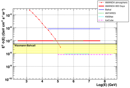
Figure 2.5: Constraints on the neutrino flux set by optical neutrino telescopes. The $\bullet$ markers represent the AMANDAII atmospheric neutrino data set, the thick solid line is the $800$ days AMANDAII sensitivity and from the same paper is an estimate of the Waxman-Bahcall neutrino flux predicted from acceleration of the highest energy cosmic rays [18]. The latest limits from the Lake Baikal experiment are plotted as the thin solid line [43]. The dashed, dotted and dash-dotted curves represent the projected sensitivities from one year of ANTARES [46], KM3NeT [47], and IceCube [18] respectively.

2.4 Radio Čerenkov Detectors

Radio Čerenkov detectors are sensitive, not to the passage of muons, but to the electromagnetic component of neutrino induced particle cascades. The optimum process for detection is a charged current $\nu_{e}$ interaction. This simultaneously initiates an electromagnetic and a hadronic particle shower from the emergent electron and hadron respectively. The two showers are in principle superimposed. In 1962 G. A. Askaryan realised that the net charge of the particle cascade, in a dense medium, will not be neutral - since positrons emitted by pair-production will annihilate in flight, leaving a negatively charged excess. Additional electro-negativity is provided by the accumulation of delta rays and Compton scattered electrons. In his paper [38] Askaryan predicts that at the maximum of an $E=10^{18}$ eV shower there is a $10\%$ electron charge excess; one can expect to observe a net $20\%-30\%$ negative charge excess.

Almost forty years after this effect was postulated came experimental confirmation. Formerly, radio emission from cosmic-ray induced particle showers was shown to be measured as a result of the geomagnetic separation of electric charges. Through the detection of photon induced cascades in $3200$ kg of silica sand, evidence for the observation of the Askaryan effect was given by correlation of the radio pulse size with the energy of a shower. Furthermore it was shown that the experimental observations were inconsistent with geomagnetic charge separation and consistent with Čerenkov emission because of the alignment of the polarisation along the shower axis and not the local geomagnetic dip [48].

A brief report of existing radio Čerenkov neutrino telescopes follows, ended by a summary of experimental limits they impose on the neutrino flux.

2.4.1 ANITA

The balloon borne ANtarctic Impulsive Transient Antenna (ANITA) experiment is a recent and innovative apparatus designed for the radio detection of CR neutrinos. An $18.4$ day flight has been achieved by a prototype, named “ANITA-lite” early in 2004. [49] The principal ANITA design features a $2\pi$ array of antennas sensitive over the frequency range $230-1200$ MHz, observing $\sim 2$Mkm³ of Antarctic ice, where the depth is equivalent to the radio attenuation length, from an altitude of $37$ km. The ANITA-lite prototype, whilst only consisting of two ANITA antennas with $12\%$ of the viewing area of the full scale detector, still observed a considerable $0.17$ Mkm³ of ice, producing competitive constraints on the UHE neutrino flux that ruled out the remaining “Z-Burst” ($\nu\overline{\nu}\to Z^{0}$) flux that was not already constrained by previous experiments, as a mechanism for the production of the highest energy CRs. Simulations of the full scale detector project a sensitivity down to sub-GZK fluxes, thus opening a window to cosmogenic neutrinos and possibly never before seen, extra galactic cosmic accelerators. A two month mission successfully launched in December 2006.

2.4.2 FORTE

Developed by the Los Alamos and Sandia National Laboratories the Fast On-orbit Recording of Transient Events (FORTE) satellite sits in a circular orbit at an altitude of $800$ km and inclined $70$ ^∘ from the Earth’s equator. Launched in 1997, its on board optical and radio frequency receivers can be exploited for the study of hadronic particle cascades in the Greenland ice sheets as well as lightning storms and for its intended use as a nuclear detonation detector. The most recent analysis of the FORTE data set contains over $4$ million events, recorded from September 1997 to December 1999[50]. Only a single event passed through each level of cuts, so the calculated flux limits for the experiment assume this to be a representation of the background level. Backgrounds are present in the form of radio emissions from lightning strikes. Certain artifacts of a lightning event can be used to reject backgrounds of this nature such as signal grouping, random polarisations and pulse pairs resulting from reflections off the ground. Lightning activity over the Greenland is however extremely rare and thus good knowledge of the geographic location of a signal can further reduce the background activity. Tentative limits have been placed on the flux of astronomical neutrinos in the energy range $10^{13}\to 10^{16}$ GeV. One treats these with caution noting that they extend beyond the scale for GUT particle masses and are calculated in the absence of neutrino-nucleon cross section data above $30$ TeV.

2.4.3 GLUE

As stated at the beginning of this chapter, it is possible to observe neutrino induced cascades that occur not in sea, ice or salt on Earth but in the lunar regolith; this is illustrated schematically in Figure 2.6. The Goldstone Lunar Ultra-high energy neutrino Experiment (GLUE) looks for radio signals from this source. This technique is facilitated by two large antennas, one $70$ m and one $34$ m in size, separated by a baseline of $22$ km. By utilising the two receivers in coincidence, with a large separation, one can in principle reduce the anthropogenic radio background. On average the background due to random coincidences and thermal noise is reported to be $3\times 10^{-3}$ Hz, resulting in a $\geq 95\%$ livetime during operation [51].

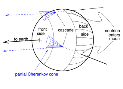
Figure 2.6: UHE cascades in the lunar regolith (from [51]).

The reported analysis incorporates a livetime of approximately $120$ hours which, although quite small, employs up to $0.1$ Mkm³ of detector material, which is enough to constrain some of the aforementioned Z-Burst and TD models. No neutrino candidate events are present in the $120$ hours data set [51].

2.4.4 LOFAR/LOPES

LOFAR, the LOw Frequency ARray, including the LOFAR PrototypE Station (LOPES), is a large scale radio telescope, being built for a broad range of astrophysical studies. One goal is the detection of CRs and neutrinos through geo-synchrotron emission and radio fluorescence in the Earth’s atmosphere and the Askaryan effect in the terrestrial and lunar regoliths [52]. The operable range of frequencies is from $15\to 240$ MHz. The cleanest channel for direct neutrino detection is through Čerenkov emission in the lunar regolith [53] in the same way as illustrated by Figure 2.6. It is predicted that the efficiency of the technique should allow for detection of neutrinos an order of magnitude below predicted GZK fluxes, after only $30$ days observation at a signal detection threshold of $500\times 10^{-26}\,\mathrm{Wm}^{-2}\mathrm{Hz}^{-1}$ [54].

2.4.5 RICE

RICE is the Radio Ice Cherenkov Experiment, at the South Pole. It was deployed in the Antarctic ice in tandem with AMANDA (section 2.3.1) and consists of an $18$ channel array of radio receivers distributed about a cube of length $200$ m. The depth of each receiver varies between $100-300$ m. Each of the dipole antennas has a dedicated, in-ice pre-amplifier before the signal transmission along a cable to the surface where background noise from local electronics and more importantly the AMANDA PMTs is filtered away. Event triggering initially requires that at least four channels register a peak above a threshold set beyond the level of thermal and background fluctuations, or that any channel registers a peak above threshold in coincidence with a $30-$fold AMANDA-B trigger. A horn antenna at the surface provides an active veto against surface generated background transient events. Raw trigger rates of $10$ Hz are reported [55] after veto. There is a reported livetime of $\sim 90\%$ after discrimination of surface transients of anthropogenic origin. Event vertices are reconstructed via the difference in arrival times of signals at successive pairs as well as a lattice interpolation algorithm; a Čerenkov cone of opening angle $57$ ^∘ is then superimposed on the vertex. A location accuracy of $\sim 5$ m is reported. Data analysis spanning records from 1999-2005 has been performed [56] yielding no events consistent with a neutrino induced cascade.

2.4.6 SALSA

The SALt dome Shower Array (SALSA) collaboration represent the greatest interest in the instrumentation of subterranean salt domes with radio antennae for the detection of ultra-high energy, neutrino induced particle cascades. To date preliminary investigations of United States sites have been undertaken as a means to surveying the suitability of naturally occurring halite deposits for use as calorimeters. Indications are that in terms of enclosed mass within one attenuation length radius, salt domes provide a competitive material to ice. Furthermore, the simple cubic-lattice structure of halite is potentially less causative of distortion through depolarisation and rotation of the signal about the plane of polarisation. Additionally halite is less birefringent than ice too. Results from a Monte Carlo (MC) simulation of an instrumented salt dome have been reported [57]. A sensitivity of the order $10$ events per year from a minimal GZK flux is expected from a $10\times 10\times 10$ antenna array on a $200$ m grid spacing. Perhaps more important is the recent experimental work that has confirmed the generation of coherent Askaryan radio pulses, in salt, as a result of a net charge excess, synthesised during the development of particle cascades [48]. As discussed at the beginning of this section, this work clearly upholds the production of radio pulses via the Askaryan effect and refutes the hypothesis of geometric charge separation as their source.

2.4.7 Limits on the neutrino flux from radio Čerenkov
neutrino telescopes

Current limits on the neutrino flux from radio Čerenkov based detectors appear in Figure 2.7. Some predicted limits are also included based on proposed extensions to existing experiments and from new projects. Plotted on the same figure are some model neutrino fluxes predicted by theory.

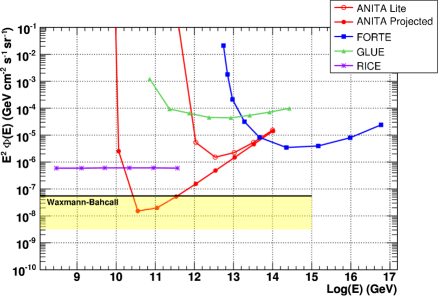
Figure 2.7: Constraints on the neutrino flux limits from radio Čerenkov detectors. The sensitivity of ANITA Lite is shown by the $\circ$ markers and the projected sensitivity of the full ANITA detector by the $\bullet$ markers [49]. The FORTE sensitivity is shown by the $\blacksquare$ markers [50]. GLUE [51] and RICE [56] are indicated by the $\blacktriangle$ and $\times$ markers respectively. Again the WB flux of neutrinos from [18] is shown.

2.5 Acoustic Detection of UHE Neutrinos

Acoustic detection of high energy particles was first postulated in 1957 [58] and subsequently full theoretical analyses of the signal production mechanism were performed (e.g. [59]). The hadronic particle cascade induced at the interaction vertex by an UHE neutrino has enough thermal energy to locally heat the surrounding medium, causing it to rapidly expand. This produces a pressure pulse, measurable on a suitable acoustic receiver. The minimum neutrino energy required for this technique lies around $10$ EeV ($10^{19}$ eV). Whilst the structure of the hadronic showers is the same for all three flavours of neutrino, the behaviour of the lepton differs. For $\nu_{e}$ type neutrinos the lepton energy is deposited as an electromagnetic cascade that is effectively detected along with the hadron shower. In the case of $\nu_{\mu}$s the resulting muon is virtually undetectable acoustically because the mean free path for catastrophic Bremsstrahlung and pair-production is of the order of several km. $\nu_{\tau}$ interactions produce a tau lepton which may or may not decay within the fiducial volume of a detector, initiating a second cascade.

2.5.1 The LPM effect

Before discussing the acoustic detection of neutrinos it is necessary to consider the dynamics of such energetic events. At EeV energies quantum interference affects the passage of leptons through a medium. The Landau Pomeranchuck Migdal (LPM) effect [60],[61] describes a suppression of the cross sections for pair production and Bremsstrahlung. This effect dominates the development of the leptonic component of a neutrino DIS event as its interaction lengths become comparable to the interatomic distances of the medium through which it propagates. An EeV electromagnetic cascade that is typically a few metres in length at TeV energies can extend to hundreds of metres because of the LPM effect. The discussion of thermoacoustic emission that follows is limited to the hadronic component of the neutrino interaction. Any acoustic emission from the electromagnetic cascade is assumed to be inaudible due to the extended nature of the source and is thus neglected.

2.5.2 Formation of the acoustic signal

The thermal energy deposition along the cascade axis occurs via ionisation and excitation of the surrounding medium and is instantaneous on the acoustic and thermal diffusion timescale. The cascade can be thought of as a series of discrete regions in which a Gaussian heat deposition occurs, resulting in an instantaneous step in temperature. The corresponding pressure wave is simply the second derivative with respect to time of the change in temperature, yielding a distinctive bipolar acoustic pulse. Because of the instantaneous development of the cascade, the acoustic radiation is emitted in phase such that individual pulses interfere. This is analogous to a line of sources emitting Huygens’ wavelets. In the far field these sources have undergone Fraunhofer diffraction such that the total acoustic radiation is confined to a narrow, so-called “pancake” with an opening angle $\theta$ of about $5$ ^∘. The geometry of the cascade and the acoustic emission is illustrated in Figure 2.8.

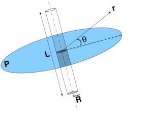
Figure 2.8: Schematic of the energy deposition. At $E_{\nu}=10^{20}$ eV, in water, a hadronic shower deposits $99\%$ of its energy in a cylinder of length $L=20$ m and radius $R=20$ cm. The energy deposition of the shower can be considered as a series of coherent sources lying along the shower axis.

Following the workings of [59] and [62] the acoustic signal production is analysed. If the energy per unit volume per unit time is given as a function $E(\mathbf{r},t)$, then the total neutrino energy is $E_{0}=\int_{V}E(\mathbf{r})d^{3}\mathbf{r}$. The wave equation for the pressure pulse produced $p$ is:

$$\nabla^{2}(p+\frac{1}{\omega_{0}}\dot{p})-\frac{1}{c^{2}}\ddot{p}=-\frac{\beta}{C_{p}}\frac{\partial E}{\partial t}$$ (2.6)

Where for seawater the parameters are:

$c$,

the speed of sound in water $\sim 1500$ ms^-1,

$\beta$,

the bulk coefficient of thermal expansion $\sim 2.0\times 10^{-4}$ K^-1,

$C_{p}$,

the specific heat capacity at constant pressure $\sim 3.8\times 10^{3}$ Jkg^-1K^-1,

$\omega_{0}$,

the characteristic attenuation frequency $\sim 25$ GHz.

It should be noted that $\omega_{0}$ is actually a function of the frequency of the radiation (it is, in fact, dependent on the sound attenuation coefficient, which is itself frequency dependent) but to keep these calculations simple it is taken as a constant for the frequency range of interest $f=10-100$ kHz. One can express the instantaneous nature of the heat deposition by $E(\mathbf{r^{\prime}},t)=E(\mathbf{r^{\prime}})\delta(t)$, where $\mathbf{r^{\prime}}$ is the location where the instantaneous heat deposition takes place. The resultant pressure wave some other location $\mathbf{r}$ as a function of time $t$ is therefore:

$$p(\mathbf{r},t)=\int_{V}E(\mathbf{r^{\prime}})G(\mathbf{r}-\mathbf{r^{\prime}},t)d^{3}\mathbf{r^{\prime}}$$ (2.7)

$G(\mathbf{r},t)$ is the pressure pulse generated by a point source $E=\delta(\mathbf{r})\delta(t)$, taking attenuation into account this is:

$$G(\mathbf{r},t)=-\frac{\beta}{4\pi C_{p}}\frac{(t-r/c)}{r\sqrt{2\pi}\tau^{3}}e^{-(t-r/c)^{2}/(2\tau^{2})}$$ (2.8)

where $\tau=\sqrt{r/(\omega_{0}c)}$.

2.5.3 Laboratory based measurements of thermoacoustic
emission

Since the thermoacoustic mechanism for detection of particle cascades was proposed [59] a number of experiments have attempted to measure the effect in the laboratory, either through the use of particle accelerator beams or high energy light sources. A discussion of two such experiments follows.

The 1979 Brookhaven-Harvard experiments

Some twenty-two years after Askaryan’s proposal of the thermoacoustic mechanism for high energy particle detection, the first experiments were undertaken at the Brookhaven National Laboratory (BNL) and Harvard University cyclotron, to record the acoustic signal emitted due to proton beams traversing fluid media. The following summary is based on the material reported in [63]. Three experimental apparatus were used:

1. The BNL $200$ MeV proton linear accelerator (LINAC) produced a beam of protons with total bunch energies between $10^{19}\to 10^{21}$ eV. The range of the beam in water was $\sim 30$ cm, with a fixed $4.5$ cm diameter. The spill time was variable between $3\to 200$ µs. The energy of the beam was not tunable.

2. The Harvard University cyclotron accelerated protons up to $158$ MeV with a beam energy that could be tuned down to $10^{15}$ eV (close to threshold for the acoustic signal). The beam had a range of $16$ cm in water with a minimum $50$ µs deposition time, which was long in comparison to the sound transit time across the diameter of the beam and thus dominated the temporal structure of the emitted acoustic signal. The beam diameter could be varied between $1\to 10$ cm.

3. A second fast extracted beam (FEB) from a $28$ GeV proton accelerator was utilised at BNL. This had a fixed beam energy of $10^{19}$ eV, with a range of $20$ cm. The diameter of the beam was variable between $5\to 20$ mm and the deposition time was short at $2$ µs. In contrast to the cyclotron experiment, where the beam spill time was the dominant effect, the sound transit time across the beam diameter dominated the temporal structure of the signal.

Each of the above apparatus had sufficient dimension to allow for resolution of the initial signal and subsequent reflections (much greater than the beam diameter or cascade length). The primary source of error was due to the uncertainty in the measurement of signal amplitudes and beam intensities. It is reported that audible clicks could be heard by the unaided ear, but this in itself did not prove the thermoacoustic mechanism. It still remained to disprove acoustic emission due to molecular dissociation and microbubble formation.

In the case of a short beam spill time ($10$ µs), where the signal transit time was $d/c=4.5$ cm/$1.5$ mm µs${}^{-1}=30$ µs in water at $20$ ^∘C, a clear bipolar signal was registered, this is plotted in Figure 2.11. The separation between this and the subsequent first reflection displayed the appropriate delay for the given geometry. The half width of the pulse was directly proportional to the transit time across the diameter of the beam and the time delay between hydrophones at two different locations was consistent with their respective path lengths. A leading compression was confirmed by placing two hydrophones $180$ ^∘ out of phase. When the beam spill time was significantly longer ($100$ µs) than the signal transit time ($30$ µs) then there was a clear separation between the leading compression and the subsequent, final rarefaction. The observed signal (Figure 2.11) is calculated as the convolution of a quasi-instantaneous pulse (Figure 2.11), and the beam spill intensity (Figure 2.11) as a function of time.

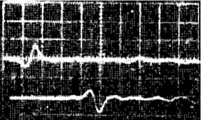
Figure 2.9: The pressure pulse observed from a $10$ µs proton beam spill (from [63]). The hydrophone producing the lower trace is $180$ ^∘ out of phase with the upper one.

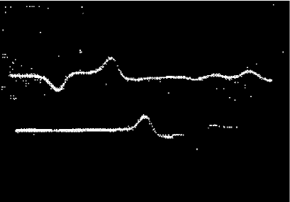
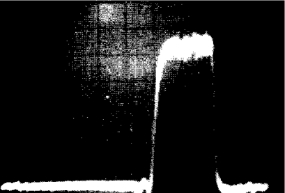
Figure 2.10: The pressure pulse observed from a $100$ µs proton beam spill (from [63]). The hydrophone producing the lower trace is $180$ ^∘ out of phase with the upper one.

Figure 2.11: Time profile of $100$ µs beam intensity (from [63]).

The signal period as a function of spill time served to act as a proof of principle for the thermoacoustic mechanism and its underlying linear theory. The level of agreement was limited to $2\sigma$ ($85\%$) due to the large errors imposed by the uncertainties in the measurements of the beam intensities and pulse heights.

Repeated tests were performed with different media such as olive oil and CCl₄ to look for deviations from the linear models as a result of excitation of ions and/or molecular dissociation. Microbubble formation was also examined by using the different media under varying combinations of temperature and pressure (so as to alter the microbubble diameters). No deviation was observed as a result of either ion excitation, molecular dissociation or microbubble formation within the $25\%$ experimental uncertainty. Furthermore the spatial dependence of signal amplitudes was shown to vary as the reciprocal of the distance away from the cascade as anticipated by the model of linear superposition in the far-field condition.

The aforementioned experiment serves as a proof of principle for the thermoacoustic model. There were large inherent uncertainties to the technique used for measuring the thermoacoustic emission from each of the accelerator beams used, constraining the agreement between the observed data and the predictions of the underlying theory only to within $2\sigma$.

Uppsala proton beam and Erlangen laser beam studies

The most recent attempt to test the predictions of the thermoacoustic mechanism [64] have utilised both a high energy ($10\to 400$ PeV total bunch energy) proton beam and an EeV pulsed infra-red ($1064$ nm) Nd:YAG laser. The proton beam, being charged, both ionises and excites the target medium but the laser beam, being neutral, will only excite target atoms. The density of pure water is maximal at a temperature of $4$ ^∘C; below this the coefficient of thermal expansion ($\beta$ in Equation 2.6) is negative. Hence an increase in temperature in pure water below $4$ ^∘C produces a compression and not an expansion. The coefficient for sea water is greater than that for pure water and increases with increasing pressure, temperature and salinity [65]. In this experiment the temperature of the target water tank was varied between $1$ ^∘C and $20.0$ ^∘C $\pm 0.1$ ^∘C. The proton beam, delivered from the $177$ MeV cyclotron at the Theodor Svedberg Laboratory in Uppsala, Sweden, had a diameter of $1$ cm and a spill time of $30$ µs. It produced a shower with approximately uniform energy deposition in water for $20$ cm, ending in a Bragg Peak at approximately $22$ cm. The Erlangen Physics Institute laser energy was adjusted between $0.1\to 10$ EeV with a fixed pulse length of $9$ ns and beam diameter of a few mm. The energy deposition of the beam, along the beam axis, decayed exponentially with an absorption length of $6.0\pm 0.1$ cm.

Acoustic pulse data from the laser produced the expected inversion, predicted by the thermoacoustic model, at $4.0$ ^∘C to within $0.1$ ^∘C. The same measurement using the proton beam however revealed an apparently temperature independent contribution to the overall amplitude, present at a level of $5\%$ of the signal at $15$ ^∘C. The results predicted by the thermoacoustic mechanism were obtained following subtraction of this artifact from the proton beam data. The source of this contribution to the acoustic signal was not verified and was identified as a topic for further investigation. A hypothesis was proposed that the extra signal was a result of the charge of the proton beam, hence it was not apparent in the laser induced pressure waves.

Whilst the results of the Erlangen-Uppsala tests still leave some unanswered questions, they appear to strengthen the support of the thermoacoustic model. It still however remains to identify the extra source of sound apparently resulting from the charged nature of the proton beam.

2.5.4 Experimental results from SAUND

The SAUND collaboration [66] have published [67] the first diffuse neutrino flux limit based on their work on a United States Navy hydrophone array located in the Tongue of the Ocean, a deep basin situated near the Bahamas. They use a seven hydrophone subset of the total $52$ hydrophone AUTEC array, arranged in a hexagonal pattern at depths between $1570$ m and $1600$ m. The spacing between hydrophones is between $1.50$ km and $1.57$ km and they are mounted upon vertically standing booms that are anchored to the seabed.

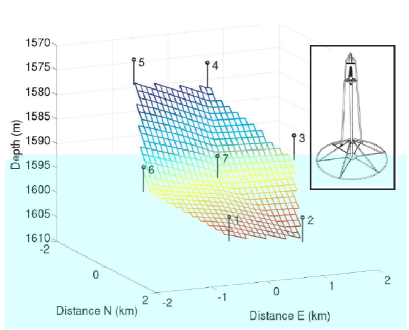
Figure 2.12: Schematic view of the hydrophone array used by the SAUND collaboration (from [67]).

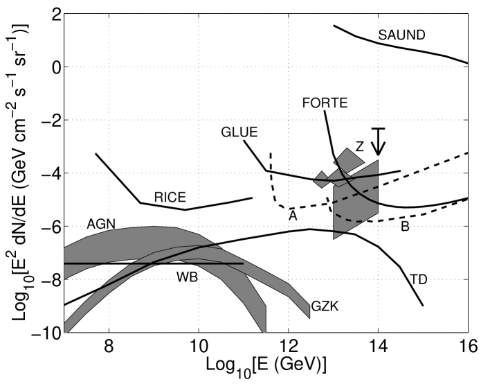
Figure 2.13: Flux limit curves for the AUTEC array (solid line labelled SAUND) and the hypothetical arrays (A and B) including the predicted flux of several theoretical models: “Z” for Z-Bursts, “TD”for Topological Defects, “WB” for the Waxman and Bahcall flux and “GZK” for the GZK theoretical flux. Some experimental limits (FORTE, GLUE and RICE) are also indicated (from [67]).

A novel technique was employed by which calibration of the hydrophones was achieved by dropping weighted light bulbs into the sea from a stationary boat at the surface. Measuring the signal as the bulb imploded under pressure gave a rough estimation of the energy sensitivity of the array to a known source and allowed for timing calibration.

In addition to the AUTEC array performance evaluation a computer simulation was developed to test the sensitivity of two hypothetical arrays. Each was comprised of hexagonal lattices of 1.5km long strings, the strings being modelled to have continuous pressure sensitivity along their entire length. Array “A” is bounded by circle of radius 5km with 500m nearest neighbour spacing. Array “B” is bounded by a circle of radius 50km, with 5km spacing between strings. The results of this work are illustrated in Fig 2.13, the next phase of this experiment “SAUND II” is currently underway.

2.6 Practical Motivation for the Acoustic Technique

The introduction hints why an astronomer would look for neutrino light: neutrinos interact only via the weak nuclear and gravitational forces. This means they can reach us from the furthest depths of the Cosmos without being deflected, illuminating parts of the universe no other particles can. The very fact that CRs exist with energies greater than $10^{20}$ eV is the greatest motivation for UHE neutrino astronomy, since there must be a neutrino counterpart to such emission. One must however convince oneself that acoustic neutrino detection can compete with existing methods and support the detection of neutrinos at the highest energies. Table 2.1 shows a comparison of signal attenuation lengths for different methods of detection.

		Water	Ice	Salt
EM Optical	(Čerenkov)	$\sim 50$ m	$\sim 100$ m	$\sim 0$ m
EM Radio	(0.1$\to$1.0GHz)	$\sim 0$ m	$\sim$ few km	$\sim 1$ km
Acoustic	(10kHz)	$\gtrsim 10$ km	$\gtrsim 10$ km	$\gtrsim 10$ km

Table 2.1: Attenuation lengths for different techniques

Acoustic detection methods can offer the largest instrumented and effective volumes since the signal propagation lengths are orders of magnitude greater than for Čerenkov detectors.

2.6.1 “Back of the envelope” comparison of effective volumes for an optical neutrino telescope and an acoustic telescope with 1000 sensors

The maximal effective volume $V_{\mathrm{eff}}$ of ANTARES to $\nu_{\mu}+\overline{\nu_{\mu}}$ is $\sim 1$ km³ [68]. ANTARES comprises approximately $1000$ sensors, instrumented in a volume of $0.03$ km³. If one assumes a regular spacing between sensors then the volume occupied per sensor is approximately $0.03/1000=3\times 10^{-5}$ km³/sensor. The simplest arrangement of these volumes is a simple cubic lattice as illustrated in Figure 2.14.

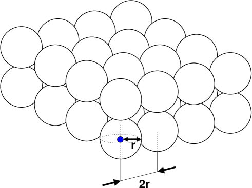
Figure 2.14: The instrumented volume is divided equally amongst each sensor. In a simple cubic lattice each sensor sits at the centre of a sphere of radius $\mathbf{r}$.

This gives a separation between sensors of:

$$\frac{4}{3}\pi r^{3} = 3\times 10^{-5}$$

$$r = 0.0192\,\mathrm{km}$$

$$2r = \sim 40\,\mathrm{m}$$

which corresponds to $80\%$ of the $\sim 50$ m attenuation length of $450$ nm Čerenkov light.

The most conservative estimate for $V_{\mathrm{eff}}$ of an acoustic array is to assume that $V_{\mathrm{eff}}=V_{\mathrm{inst}}$ where $V_{\mathrm{inst}}$ is the volume instrumented by the detector. If one populates a volume equivalent to $1000$ acoustic sensors separated by $80\%$ of an again conservative $10$ km attenuation length for sound:

$$\frac{4}{3}\pi r^{3} = \frac{V_{\mathrm{eff}}}{1000}$$

$$V_{\mathrm{eff}} = 1000\times\frac{4}{3}\pi(8/2)^{3}$$

$$V_{\mathrm{eff}} = 85333\mathrm{km}^{3}$$

Remember, we have already been conservative in our approach, and have shown that if $V_{\mathrm{eff}}=V_{\mathrm{inst}}$ for an acoustic sensor array, it can have an effective volume $\sim 85000$ times greater than an optical array, with the same number of sensors. It has, however, been suggested that an acoustic array can experience $V_{\mathrm{eff}}$ up to one hundred times greater than $V_{\mathrm{inst}}$ [69], which would then give a $85\times 10^{5}$ times larger effective volume for an acoustic array over an optical.

caveat

The Optical Modules in ANTARES are not spaced on a regular cubic lattice, the exact geometry is complex and is dependent on reconstruction requirements, but since the reconstruction requirements of our hypothetical acoustic array are unknown, we give both detectors an equivalent geometry and an equivalent sensor separation as a function of signal attenuation. Similarly positioning acoustic sensors with a separation of $10$ km, just because of the long attenuation lengths of sound, neglects any requirement for reconstruction.

In conclusion, an acoustic array can potentially have an effective volume of the order $85\times 10^{3}\to 85\times 10^{5}$ times greater than an optical array with an equivalent number of sensor elements, neglecting requirements for reconstruction. In the following chapters, for historical reasons, typically one thousand acoustic sensors are considered in a volume of one cubic kilometre, a considerably denser population than argued here. However, as the discussion progresses a sparser optimum sensor density, taking into consideration reconstruction requirements will be considered.

2.7 Summary

Three methods of detecting cosmological neutrinos have been discussed. Each one is at a different level of maturity yet all are proving fruitful. Figure 2.15 incorporates the present and predicted sensitivities from Figures 2.5 and 2.7 into an illustration of the energy ranges for each method of detection. The expected energy range of acoustic detection is also included. The case for the development of acoustic detection lies firstly in its sensitivity to the highest energy neutrinos, thus completing the study of the entire neutrino energy spectrum, and secondly, the ability of the acoustic technique to deliver detectors with vast effective volumes.

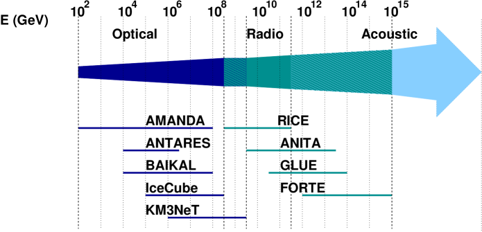
Figure 2.15: The range of neutrino energies detectable by each technique illustrated in terms of the existing and projected sensitivities of several neutrino detection experiments.

Chapter 3 Simulating Neutrino Interactions

3.1 Introduction

This chapter deals with the simulation of neutrinos colliding into the Earth at energies of several Joules. It describes the first links in the simulation chain that ultimately predicts the sensitivity of a hypothetical array of underwater acoustic sensors to a flux of ultra high energy neutrinos. The first section discusses the underlying event - the neutrino deep inelastic scatter, the second section describes simulation of the induced particle shower and the final section describes how the acoustic signal is generated as a result of the thermal energy deposition of the hadronic cascade.

3.2 Neutrino Event Generation

The kinematics of neutrino deep inelastic scattering were introduced in the opening paragraphs of Chapter 2. In order to determine the contribution of the neutrino energy to the induced hadronic cascade it is necessary to compute the Bjorken-$y$ dimensionless scaling variable. Physically $y$ describes the fraction of the incident neutrino energy that is carried away by the hadronic system.

The All Neutrino Interaction Simulation (ANIS) [70] has been developed for analysis of data from the AMANDA [39] neutrino telescope. It is a fully object oriented C++ toolkit, utilising the CLHEP vector class and HepMC event records [71]. The program generates neutrinos of any flavour according to a specified flux and propagates them through the Earth eventually forcing them to interact in a specified volume should they not be attenuated en route. The propagation of low energy ($<10^{3}$ GeV) neutrinos through the Earth’s crust and the attenuation of neutrinos at high ($>10^{9}$ GeV) energies is plotted in Figure 3.1. The range of neutrinos, through the Earth’s crust, at low and high energy is plotted in Figure 3.2.

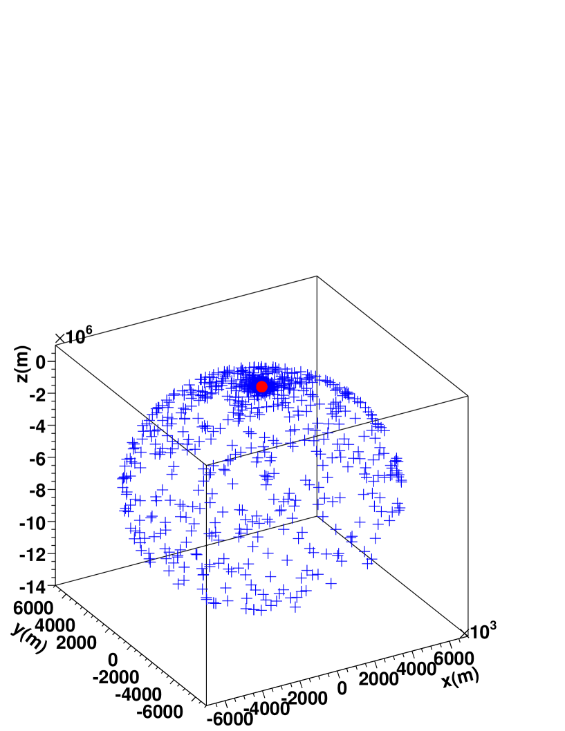
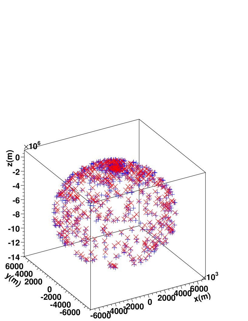
Figure 3.1: Low energy neutrinos (Left) propagate freely from the surface of the Earth ($+$ markers), through the crust to the fiducial volume ($\bullet$ marker) where they are forced to interact. High energy neutrinos (Right) do not travel far from their point of origin ($+$ markers) before they are attenuated by the crust ($\times$ markers). This demonstrates the increase in the neutrino nucleon cross section with neutrino energy.

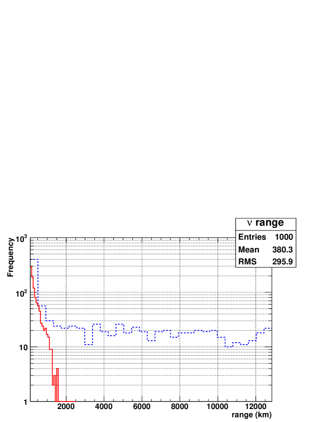
Figure 3.2: Range of neutrinos in ANIS at $1<E_{\nu}<10^{3}$ GeV (dotted) and $10^{9}<E_{\nu}<10^{12}$ GeV (solid). The low energy neutrinos can penetrate up to the full diameter of the Earth $\sim 12000$ km before they are forced to interact, whereas high energy neutrinos are attenuated by about $2000$ km of rock.

It is assumed that all neutrinos interact in a fiducial volume, a cylindrical “can” surrounding the volume instrumented by hydrophones. The energy spectrum is assumed to be flat in $\log E$, hence $dN/dE\propto E^{-1}$. Only neutrinos originating from a positive hemispherical shell (with its origin at the centre of the instrumented volume) are considered. Hence the ANIS program need only propagate neutrinos through the detection medium (water) and not through the Earth’s crust.

The mean fraction of the neutrino energy imparted to the hadronic cascade is approximately $25\%$, however, the actual value can vary from $0-100\%$. This is shown in Figure 3.3, and is assumed to be independent of neutrino energy. Initially in this simulation all hadronic cascades are assumed to contain $25\%$ of the energy of the incident neutrino, since vertex reconstruction relies on the timing and not the magnitude of a pressure pulse. The effect of a non constant $y$-value will be discussed in Section 5.8 later when describing attempts to reconstruct the energy of a neutrino from a given event.

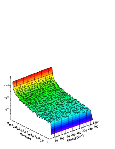
(a) Energy dependence

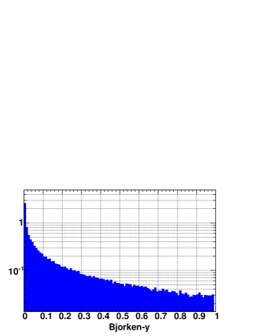
(b) Bjorken-$y$ probability density for all energies

Figure 3.3: Bjorken-$y$ probability density for three flavours of neutrino in the energy range $10^{8}\to 10^{12}$ GeV, interacting in water. As indicated by plot 3.3(a) the shape of the probability density is independent of the neutrino energy. Plot 3.3(b) is the three flavour $y$-distribution averaged over all energies between $10^{8}\to 10^{12}$ GeV (i.e. a projection of plot 3.3(a) along the energy axis).

There is one remaining issue to be addressed at this stage of the simulation, that of event multiplicity. In the section that follows it is assumed that the hadronic cascade is initiated by a single excited hadron that, following the neutrino DIS, carries $25\%$ of the energy of the incident neutrino. More accurately there will be some small number of excited partons between which this percentage of the neutrino energy is shared; however, ANIS restricts itself to calculation of the energy of the excited hadronic final state and not the parton content.

A comparison of Bjorken-$y$ distributions from ANIS and two other event generators, namely PYTHIA and a bespoke program developed for the ACoRNE collaboration, (see [72]) has been made. The results in Figure 3.4 indicate that the produced distributions are consistent.

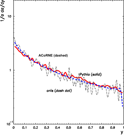
Figure 3.4: Bjorken-$y$ distributions at $10^{5}$ GeV from different event generators.

3.3 Simulating Neutrino Induced Particle Cascades

3.3.1 Physics processes

Given an expression for the energy of the hadronic system one can proceed to simulate the development of the subsequent particle cascade within a given material. A suitable particle physics toolkit for simulating the passage of particles through matter is Geant4 [73]. There are three categories of physics model at the heart of this program: those driven by theory; parameterised models which combine theory and data; and empirical physics models driven purely by data. The user is required to choose which physics models and which cross-section data are used in a given energy range. Two models can overlap in energy so long as one model does not fully occupy the same total energy range as another. A set of ready made high energy calorimetry “physics lists” are distributed with the Geant4 source code. Conceptually the formula for construction of a physics list is as follows:

$$\textsf{physics list}=\textsf{particles}+\textsf{processes}+\textsf{cross-sections}$$ (3.1)

Unless a particle is assigned a process it will do nothing in the simulation. If a particle is assigned more than one process then the processes compete. One process may invoke many models and each model has a default cross-section. It is first determined when and where a process should occur, which depends on interaction length and cross-section; secondly the final state is generated, which is dependent on the model invoked.

3.3.2 Particle production thresholds

A particle propagates through the simulated detector losing energy via the production of secondary particles. There must be some energy below which a particle no longer produces secondaries otherwise the program will suffer from infrared divergence. Hence the user must impose an energy threshold cut. However, such a cut may result in a poor estimation of the stopping location and energy deposition of the particle, so, the cut is made on the particle’s range instead. The range cut is the same for all materials but the corresponding energy threshold is material dependent. Once a particle reaches the energy below which no further secondaries are produced it is tracked to zero energy through a continuous energy loss mechanism.

In order to generate the thermal energy density $E(\mathbf{r}^{\prime})$ required by the pressure field integral in Equation 2.7 one initiates a shower simulation with a single proton at an energy corresponding to $25\%$ of the neutrino energy. The energy deposited by each successive interaction in the simulation is recorded in a ROOT[74] ntuple that can be analysed offline. As the shower ages its composition tends toward electrons and gamma rays through pion decay; the range cuts chosen for water correspond to a $3$ MeV energy threshold for tracking of e^± and $\gamma$. Below this energy no further secondaries are produced (a gamma for instance will no longer pair-produce) and the particle is forced to deposit the remainder of its energy continuously. This dramatically reduces CPU time and prevents the ntuple file size from diverging.

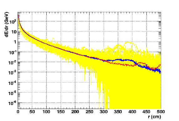
(a) Radial Energy Deposition

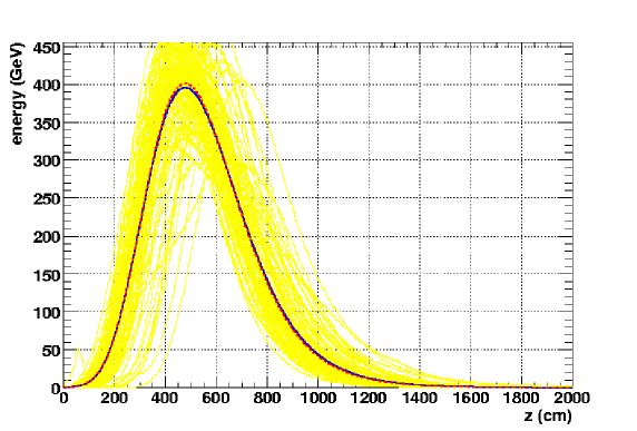
(b) Longitudinal Energy Deposition

Figure 3.5: Average radial (Figure 3.5(a)) and longitudinal (Figure 3.5(a)) energy profiles for one hundred $100$ TeV Geant4 proton showers with (solid) and without (dotted) range cuts.

The plots in Figure 3.5 illustrate the shape of the energy deposition with or without cuts applied. Whilst the effect on the shower shapes is negligible when compared to individual shower fluctuations (on top of which the average distributions are superimposed) the CPU time per event decreases from $\mathcal{O}\,20$ hours to $\mathcal{O}\,20$ minutes at $100$ TeV. Furthermore the low energy extremes of the shower (where the agreement is less good) have little effect on the resulting acoustic pulse, the shower core being the dominant contributor.

Four theory driven high energy hadronic calorimetry “use-by-case” physics lists are provided with the Geant4 distribution. They are composed of the Quark Gluon String (QGS) model or the FRITIOF (Lund string dynamics) model [75] combined with either Pre-Equilibrium or Chiral Invariant Phase-space (CHIPS) decay modes. The range of validity for each model extends from $10$ GeV to $100$ TeV. The effect of each physics list on the radial and longitudinal shower shapes is shown in Figures 3.6 and 3.7 respectively.

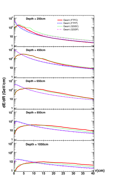
Figure 3.6: Average radial energy deposited per $20$ g cm^-2 vertical slice per unit radial distance for one hundred proton showers at $100$ TeV, using each of the high energy hadronic calorimetry physics lists. Depth refers to the distance along the shower axis.

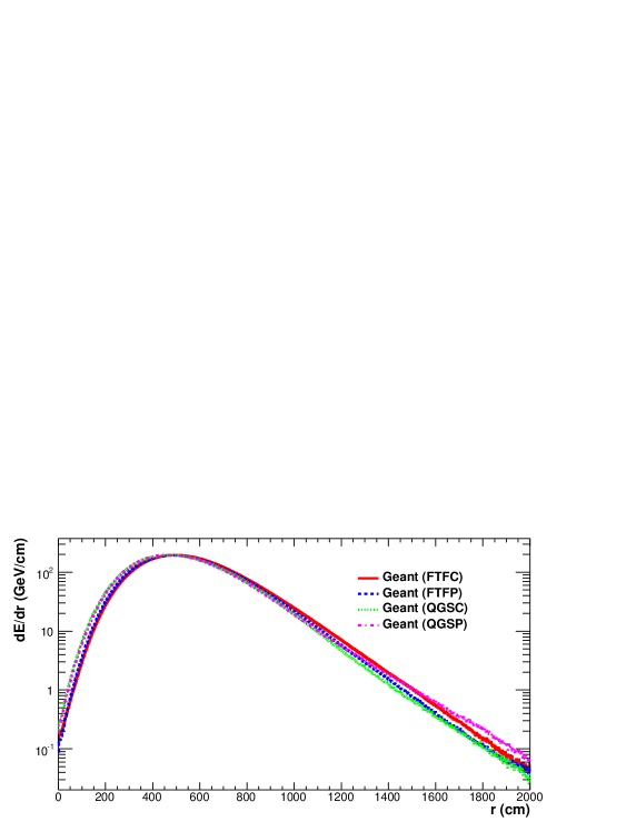
Figure 3.7: Average longitudinal energy deposition of one hundred $100$ TeV proton showers, at various depths along the longitudinal axis of the shower, using each of the high energy hadronic calorimetry physics lists.

The CHIPS decay mode tends to produce a broader, older shower, with a central energy “hole” in comparison to the pre-equilibrium decays, whilst there is little to distinguish between the QGS and FRITIOF hadron interaction schemes. References for these models can be found, for example in [76], [77], [78] and [79], as cited in the Geant4 documentation. The Pre-Equilibrium model is favoured over CHIPS since it is more consistent with the distributions seen in UHECR air showers and it is the model preferred by other groups undertaking acoustic studies. Comparisons of the longitudinal and radial shower shapes produced by Geant4 and a modified version of the CORSIKA air shower program are plotted in Appendix B.

3.4 Formation of the Acoustic Signal

The acoustic signal resulting from a hadronic cascade is computed by integrating the energy contained in the ROOTntuple as produced by the Geant4 simulation according to Equation 2.7. A typical pulse resulting from a $100$ TeV proton induced shower is plotted in Figure 3.8.

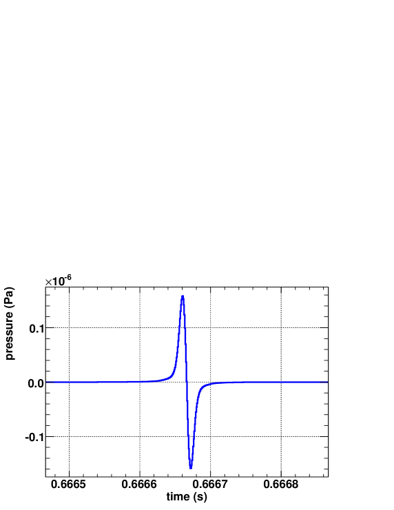
Figure 3.8: The pressure pulse for a $100$ TeV proton induced Geant4 shower in seawater, at a distance of 1km from the cascade. The angle with the plane transverse to the shower direction is $0$ ^∘.

For the purpose of simulating the performance of large scale hydrophone arrays it is necessary to determine a relationship between the energy of a neutrino and the resulting pressure amplitude at a given location. The shape of the cascade energy density becomes more uniform with increasing energy. The integrated energy of the cascade scales linearly with the energy of the neutrino; hence, the magnitude of the resultant pressure signal is assumed to scale with the energy of the neutrino. Consequently an analytical parameterisation is sought to relate peak pressure amplitude to neutrino energy. The details of how this parameterised pressure is attenuated as it propagates from the cascade to a given hydrophone is discussed in the next chapter. The peak pressures at $1$ km from various proton induced Geant4 cascades at energies in the range $10^{3}\to 10^{5}$ GeV are plotted as a function of the proton energy in Figure 3.9. A linear function is fitted to the values allowing for a direct determination of the peak pressure at $1$ km from an arbitrary shower for a neutrino of a given energy. The gradient indicates a mean pulse peak pressure of $2.12\times 10^{-11}$ Pa per GeV of thermoacoustic energy. The subsequent pulse at each hydrophone location is suitably scaled and then the effects of attenuation are applied.

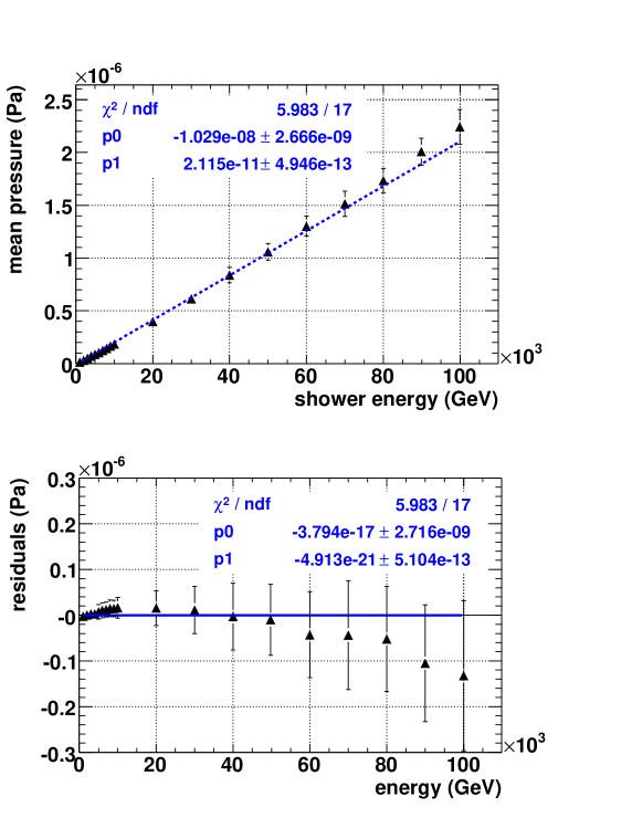
Figure 3.9: Plot of mean peak pulse pressure against energy of the hadronic shower demonstrating the linear relationship between the two. Error bars are of magnitude $1\sigma_{mean}$. The residuals plot shows the deviation of the data points from the fitted function, there is an inherent instability at higher energy due to the limited accuracies of the models used (see Appendix B).

3.5 Summary

From the simulation of UHE neutrino interactions we have learnt that approximately $25\%$ of the energy of a neutrino is carried away by the hadronic component of neutrino-nucleon deep inelastic scatter. It is therefore assumed that the particle cascade, and subsequent thermoacoustic energy deposition, induced by a neutrino with energy $E_{\nu}$, is equivalent to that produced by a proton at $E_{\nu}/4$. Furthermore, from the simulation of the evolution of TeV proton showers in the sea, we have learnt that the peak pressure of an acoustic pulse resulting from such a shower at a given distance, scales linearly with the energy contained in the shower. These findings equip us with a parameterisation allowing us to estimate the peak pressure $p$ of a pulse at $1$ km from a particle cascade initiated by a neutrino of energy $E_{\nu}$ given by:

$$p=0.25\times k_{\nu}\times E_{\nu}$$ (3.2)

where $k_{\nu}$ is the conversion constant and is equal to $21.15\times 10^{-21}$ Pa eV^-1. The parameterisation in Equation 3.2 will be used in the remainder of the simulation chain discussed in the chapters that follow.

Chapter 4 Simulating the Propagation of the Acoustic Signal

4.1 Introduction

Thus far it has been reported how the mechanisms which give rise to the distinctive bipolar pressure pulse, expected following an UHE neutrino interaction in the sea, are computed. This Chapter subsequently introduces parameterisations of signal attenuation resulting from its propagation through seawater. Incorporated into this attenuation are the effects of refraction, resulting from variation in sound velocity in the sea, and the effects of ambient noise and filtering.

4.2 Attenuation of the Acoustic Signal

A hydroacoustic pressure wave is attenuated as it propagates away from its point of origin. There are three contributions to this attenuation: a geometric factor whereby the pulse diminishes the farther it travels, a diffractive attenuation that is a consequence of the coherent nature of the acoustic emission, and the attenuation of the pulse due to the bulk mechanical properties of the medium through which it propagates. Each of these effects is discussed below.

4.2.1 Geometric attenuation

As described in Section 2.5.2 the development of the particle cascade occurs instantaneously on the thermal diffusion timescale. The result of this is coherent emission along the shower axis. In the far-field ($r\gg l$ where $r$ is the distance from the interaction and $l$ is the cascade length) the geometric attenuation of such emission goes as the reciprocal of the distance travelled [59].

4.2.2 Attenuation by the medium

The second contribution to the attenuation of the acoustic radiation, produced by a neutrino induced particle shower, is governed by the bulk mechanical properties of the medium through which it traverses. Water is a low-pass filter, high frequency components being readily attenuated, this can be seen in the sound attenuation co-efficient plot from Lehtinen et al [62] shown in Figure 4.1. For the purposes of the large scale detector simulation the attenuation was parameterised by a fourth order polynomial and recomputed for a Mediterranean water temperature of $25$ ^∘C. The effect of this attenuation on a bipolar signal is shown in Figure 4.2.

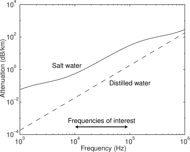
Figure 4.1: The sound attenuation coefficient for seawater (from [62]). Also shown is the absorption coefficient for distilled water.

The primary reason for the difference in absorption coefficient between seawater and distilled water is the excitation of magnesium sulfate and boric acid molecules that are present in seawater. Such molecules can have multiple stable states and transitions between states can be induced by a change of pressure, effectively converting hydroacoustic pressure into heat.

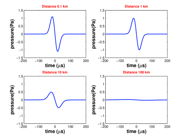
Figure 4.2: Variation of pulse shape with respect to distance, due to seawater absorption, for a signal normalised to $1$ Pa at $100$ m from the particle cascade.

4.2.3 Angular spread

As one moves out of the plane perpendicular to the shower axis, that is, the plane of the pancake, the acoustic radiation, and hence pulse pressure, is attenuated due to diffractive effects. This frequency dependent process both diminishes the pulse height and broadens the pulse width. For each frequency component of the attenuated pulse, there is a corresponding $\sin(x)/x$ diffraction pattern, in analogy to the diffraction of light through a narrow slit. The length of the shower corresponds to the size of the aperture. The pulse at zero degrees out of the pancake plane is computed by taking the Inverse Fourier Transform (IFT) at zero angle. The pulse at a given angle out of the pancake plane is thus computed by taking the IFT of the respective $\sin(x)/x$ function for that angle [81]. This effect is plotted in Figure 2. The pulse amplitude is attenuated to nearly one thousandth of its original magnitude at $5$ ^∘ out of the pancake plane for a $10$ m long shower.

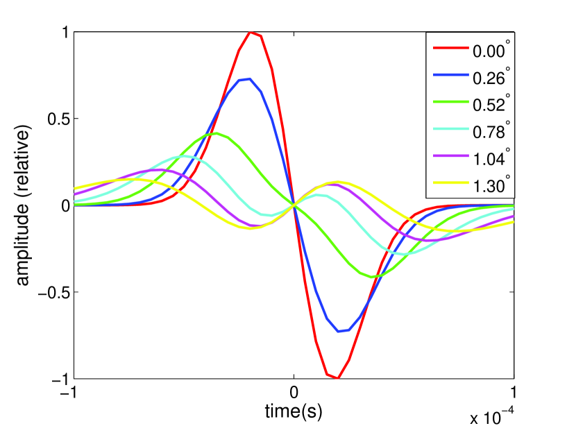
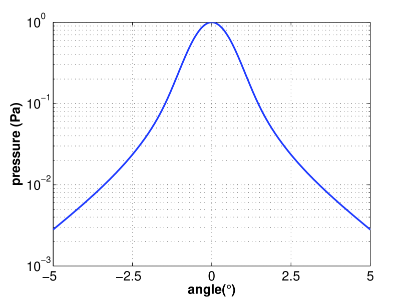
Figure 4.3: Variation of far-field pulse shapes (Left) and signal amplitudes (Right) as a function of angle out of the plane of the pancake (from [81]). The step in angle of $0.26$ ^∘ derives from the digitisation of the sample into $1024$ bins, which was chosen because it facilitates a faster IFT algorithm in MATLAB .

The angular distribution plotted in Figure 2 is parameterised and then used to scale the peak pressure recorded on a given receiver as a function of its angle out of the plane perpendicular to the shower.

The three components of attenuation described above are applied in succession to the unattenuated peak pressure amplitude as calculated via the linear energy to pressure relation formulated in Section 3.4. Given a formalism for calculating the attenuation of an acoustic pulse, as a function of the distance it propagates through the sea, a method for determining the distance travelled is desired.

4.3 Refraction

The velocity of sound in seawater is dependent on temperature, pressure, and salinity. A simple means to describe the stratification of the sea into horizontal layers of constant sound gradient is illustrated in Figure 4.4. There are three zones of sound propagation to consider: near the surface there exists an isothermal layer which is well mixed by surface waves and wind, within the isotherm the sound velocity increases with depth due to a slight increase in pressure; below the isotherm is a region known as the thermocline through which the sound velocity decreases with depth due to the corresponding decrease in temperature; below the base of the thermocline, in the deep ocean zone, the sound velocity gradient inverts and sound velocity increases with depth due to the corresponding increase in pressure.

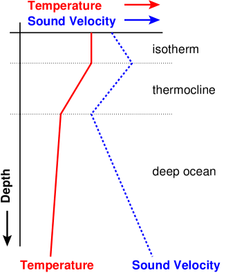
Figure 4.4: Three layers representing regions of constant sound gradient in the sea: the isotherm, the thermocline and the deep.

Sound rays tend toward the region of lowest sound velocity. Where there is an inversion in the sound velocity gradient sound rays are refracted away from each other, leading to the formation of “shadow zones”, regions from where acoustic signals may be inaudible. When building an acoustic neutrino telescope it is desirable to be far away from such environments since this will contribute to a loss in effective volume.

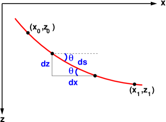
Figure 4.5: Geometry of a single curved ray in a medium with varying sound velocity.

A full derivation of the ray tracing equations in the general case, where the sound velocity gradient is not linear, and for the case of a linear sound velocity gradient can be found in Appendix C. For the geometry illustrated in Figure 4.5 with a constant sound velocity gradient $g=dc(z)/dz$, it can be shown that:

$$x_{1}-x_{0} = \frac{c_{0}}{g}\Big{(}\frac{\sin\theta_{0}-\sin\theta_{1}}{\cos\theta_{0}}\Big{)}$$ (4.1)

$$s_{1}-s_{0} = \frac{c_{0}}{g\cos\theta_{0}}(\theta_{0}-\theta_{1})$$ (4.2)

$$z_{1}-z_{0} = \frac{c_{0}}{g\cos\theta_{0}}(\cos\theta_{1}-\cos\theta_{0})$$ (4.3)

$$t_{1}-t_{0} = -\frac{1}{g}\ln\Big{\{}\frac{\cos\theta_{0}(1+\sin\theta_{1})}{\cos\theta_{1}(1+\sin\theta_{0})}\Big{\}}$$ (4.4)

where $c_{0}=c(z=0)$ is the sound velocity at the origin depth, $t_{0}$ is the time at the point of origin and $t_{1}$ is the time at point $(x_{1},z_{1})$. Angles $\theta_{0}$ and $\theta_{1}$ are the angles the ray makes with the horizontal at points $(x_{0},z_{0})$ and $(x_{1},z_{1})$ respectively; $s_{0}$ and $s_{1}$ define the arc length along the ray. For simplicity the problem has been reduced into two dimensions defining the $xz$-plane (since refraction only occurs in the vertical ($z$) direction one can arbitrarily align rays along one of the horizontal axes). The ray tracing algorithm iterates in steps of $x$ for a given path between source (cascade) and receiver (hydrophone). Equation 4.2 can be solved for the deflection angle $\theta_{1}$ which then forms the input to Equation 4.3 along with $\theta_{0}$ which is known.

In order to compute the trajectory of the real refracted ray $R$ that intersects source and receiver at $(x_{0},z_{0})$ and $(x_{1},z_{1})$ respectively one must first compute the angle of deflection $\theta_{d}$ of the deflected ray $d$ that results from sending a ray along the imaginary linear path $i$. This is because only the sound velocity as a function of depth, the coordinates $(x_{0},z_{0})$ and $(x_{1},z_{1})$; and the angle $\theta_{i}$ are known a priori.

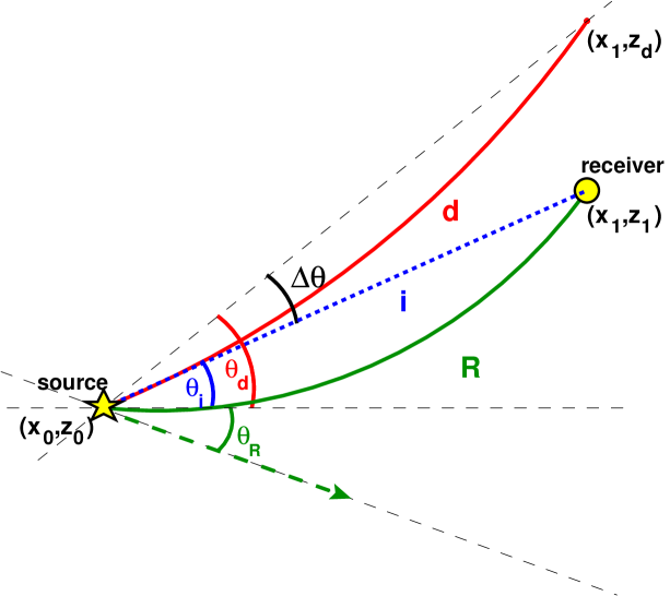
Figure 4.6: The difference between the angle of deflection $\theta_{d}$ of the deflected ray $d$ and the start angle $\theta_{i}$ of the undeflected imaginary ray $i$ is $\Delta\theta=$ $\theta_{d}$$-$$\theta_{i}$. The start angle for the real refracted ray $R$ is therefore given by $\theta_{R}$$=$$\theta_{i}$$-\Delta\theta$.

A plot of the ray trace as computed in the large scale detector simulation as described in Chapter 5 is shown in Figure 4.7.

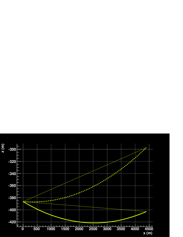
Figure 4.7: A ray trace from the large scale detector simulation. The solid curved ray and the dashed curved ray correspond to the rays $R$ and $d$ respectively in Figure 4.6.

In the case of a constant sound velocity gradient:

$$g =$$ constant

$$c = c_{0}+gz$$

where $c$ is the sound speed at depth $z$ and $c_{0}$ is the sound speed at $z=0$. The values for $c_{0}$ and $g$ are obtained from a sound velocity profile (SVP) for a particular location in the sea. The SVP at the site of the ANTARES neutrino telescope is shown in Figure 4.8 superimposed on a ray trace for a source emitting from a depth of $1500$ m at various angles to the horizontal. The effect of the inversion in the sound velocity gradient at the base of the thermocline is included, hence rays are refracted back toward the sea bed as they approach the surface. In the hydrophone array simulation only the deep sea zone, with approximated linear SVP, is considered, such that there is no inversion in the sound velocity gradient and rays are terminated at the surface without reflection. Similarly rays that hit the sea floor are terminated without reflection. This represents a more conservative approach than one where boundary reflections are considered, since the effective volume will increase if rays can reach a given array via surface or sea floor reflections. Detailed information of the boundary conditions is required to effectively model ray reflection, hence it is presently neglected.

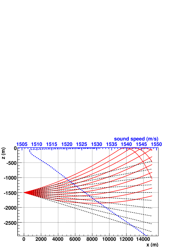
Figure 4.8: Ray trace for a source at $1500$ m depth. Refracted rays (solid) and unrefracted rays (dashed) are shown. The SVP for the ANTARES site is also shown, with sound speed across the upper $x$ axis. The ANTARES SVP is essentially linear. Neglecting the inversion in the sound speed gradient equates to extrapolating the linear section directly to the upper $x$-axis (This yields $c_{0}=1506$ ms^-1 and $g=(-)0.0156$ s^-1).

In the simulation the hydrophone array sits at $-2$ km in the deep ocean zone, far away from the thermocline in a region where the sound velocity gradient is linear. The effect of a linear sound velocity profile is to send acoustic rays along circular trajectories [82] of radius $R=c_{0}/g=1506/0.0156\sim 93$ km. There exists a natural upper limit on source distance, due to refraction, in a sea of finite depth and constant sound velocity gradient. The concept is illustrated in Figure 4.9; sources greater than $48$ km beyond an array located at mid depth in a $4000$ m deep sea cannot be detected. This is the absolute maximum distance from which a source can be heard due to the geometrical constraints of refraction. With respect to the performance of an acoustic array, by demanding several signals in coincidence, which are themselves emitted subject to angular constraints, it is unlikely a neutrino induced particle cascade could be successfully reconstructed at a distance of this magnitude. The exact limit on the distance from which cascades can be reconstructed is of importance when calculating the effective volume of a given hydrophone array and will be discussed further in Section 5.5.

Successful computation of curved ray trajectories thus allows the calculation of hit times and ray path lengths from Equations 4.2 and 4.4 respectively. The effect of attenuation as discussed in Sections 4.2.1 to 4.2.2 is thus applied to the refracted times and ray paths.

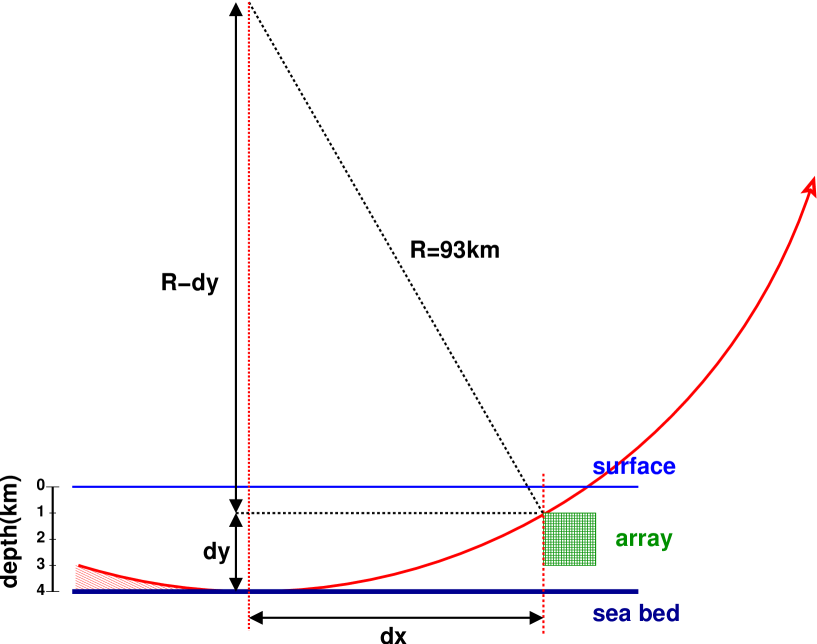
Figure 4.9: Rays following circular trajectories of radius $R=93$ km and originating from the shaded zone and beyond cannot reach the array. Hence there is a natural distance $D=2\,dx$ beyond which sources cannot be heard (so long as rays are not reflected and any inversion in the SVP is neglected, as is the case here). The Mediterranean has a maximal depth of about $4$ km, ideally an array would sit equidistant between the base of the thermocline and the sea bed. In this simulation the isotherm and thermocline are neglected along with surface and sea-bed reflections, and the array sits at mid depth. $dx=\sqrt{R^{2}-(R-dy)^{2}}$, yielding a value for $D=2\times dx=2\times 24=48$ km.

4.4 Ambient Noise, Filtering and Thresholds

Estimation of the sensitivity of a hydrophone array relies on reconstruction of the neutrino interaction vertex from the acoustic signals received. Since it is the timing of the signals that is of importance in the detector simulation, a parameterisation of neutrino energy to peak pressure can be used. In reality event triggers will depend on knowledge of the bipolar pulse shape. The performance of a matched filter is coupled to the attenuation calculation introduced in Section 4.2.3 as a means of simulating the response of a hydrophone to bipolar signals. The matched filter is applied to a flat, Gaussian white noise background. The noise level is determined from Knudsen curves (see Appendix A.2) which relate the surface wind speeds to the level of ambient noise. The matched filter enhances the signal by approximately a factor of three. The simulated hydrophones are modelled to have omnidirectional sensitivity; an example of matched filter performance is plotted in Figure 4.10. Naturally the precise shape of a bipolar signal in the sea varies as a result of the attenuation described in Section 4.2. As such a particular matched filter will be optimal for some function of distance and angle from a given source. In reality several matched filters will have to be used to fully optimise neutrino signal identification. This ensemble of filters can be represented in the large scale simulation by a single entity, optimised for all frequencies, with a probability for correct identification of a neutrino induced signal equal to unity.

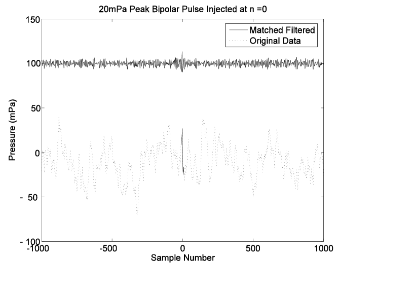
Figure 4.10: The effect of a matched filter on a bipolar signal embedded in some Rona data (from [83] which contains a full description of the matched filtering technique). The effect of such a filter on a signal embedded in a flat, Gaussian, white noise background is to enhance signal to noise by approximately a factor of three; this is the case in the large scale detector simulation. The lower plot is the raw input with the bipolar signal emboldened because it is difficult to distinguish by eye from the noise. Offset above is the filtered output, where the bipolar signal is clear relative to the background noise.

The signal detection threshold, in the detector simulation, is set at $35$ mPa, which corresponds to a probability of false alarm (PFA) of one false trigger in ten years, due to noise exclusively resulting from surface wind speed, with a five-fold coincidence. A threshold of $35$ mPa indicates a mean noise level of $35.9$ dB. The mean noise level from June to August in the Tyrrenian Sea for example is $35$ dB with an average wind speed of $5.6$ knots[80].

4.5 Summary

We have seen that acoustic radiation is modified by its transmission through the sea. This leads to a set of constraints on the simulation of a large scale acoustic array. Hydrophones that are greater than $5$ ^∘ out of the plane defined by the acoustic pancake are neglected because of the signal attenuation resulting from diffraction. There is a natural, geometry dependent, limit on the distance from which a source can be heard by a hydrophone located in a sea of finite depth because of the refraction of sound rays towards the surface. Finally, a threshold for detection of $35$ mPa has been established based on the ambient noise in the sea and the probability that this noise could emulate a neutrino like acoustic signal.

Chapter 5 Large Scale Detector Simulation

5.1 Introduction

All the ingredients are now available for the recipe that computes the sensitivity of a hypothetical array of hydrophones to a flux of UHE neutrinos. In summary the following steps have been described:

• Generation of the mean fraction of the incident neutrino energy taken away by the hadronic particle cascade.

• Simulation of the evolution of a hadronic cascade through seawater, yielding the thermal energy density deposited therein.

• Integration of the cascade energy and subsequent production of the bipolar acoustic signal.

• Parameterisation of the pulse formation process for fast calculation of peak acoustic pressure using the far-field approximation.

• Modelling of the attenuation of acoustic radiation as it permeates the surrounding seawater thus diminishing the peak pressure.

• Calculation of the trajectories and signal times for sound rays undergoing refraction due to a gradient in the sound velocity as a function of ray depth.

The following discussion explains the procedures undertaken in a bespoke simulation for the purpose of estimating hypothetical hydrophone array performances.

5.2 The Sensitivity Estimation Procedure

The steps taken by the large scale detector simulation are as follows:

Step 1.

An ensemble of downward going neutrinos is generated with an energy spectrum linear in $\log_{10}E_{\nu}$.

Step 2.

A hydrophone array is “constructed” in a deep sea environment from a file containing the coordinates of typically one thousand hydrophones distributed at random in a volume of one cubic kilometre.

Step 3.

The program then samples the neutrino spectrum and calculates the detector response on an event by event basis:

1. Each neutrino is forced to interact in a fiducial volume, called the “can”, that surrounds the volume defined by the hydrophone locations.

2. The peak pressure as a function of neutrino energy and attenuation at each hydrophone is calculated for both refracted and unrefracted sound rays assuming an omnidirectional sensitivity.

3. The pressure amplitude and arrival time for all those hydrophones that register a signal above threshold is recorded, taking into consideration the performance of a matched filter.

Step 4.

For those events that register hits above threshold reconstruction of the interaction vertex and the neutrino trajectory is attempted.

Step 5.

If the vertex reconstruction algorithm returns an unphysical vertex location the event is discarded, otherwise the event is classified as detected.

Step 6.

The sensitivity of the hydrophone array under examination is then calculated from the number of successfully reconstructed events. This is translated into a limit on the neutrino flux assuming that the hydrophone array detected no events for a given period of observation.

An example of the source distributions from which the event data are sampled can be found in Appendix D. Since we are operating close to threshold, a hard cut can be placed on the angle of a given receiver with respect to the plane of the pancake such that above $5$ ^∘ or so the receivers are neglected since the angular attenuation has diminished the signal by several orders of magnitude (see Section 4.2.3).

5.3 Neutrino Spectra and Geometries Used

As with the neutrino event generation program discussed in Section 3.2 the neutrino energy spectrum is arbitrarily modelled to be flat in $\log E$ since the ensuing sensitivity calculation will incorporate a model independent neutrino flux. Therefore:

$$\frac{dN}{d(\log E_{\nu})}=\textrm{constant}\Leftrightarrow\frac{dN}{dE}\propto E^{-1}$$ (5.1)

The neutrinos are isotropic over a hemispherical shell that is centred at the origin of the instrumented volume. All neutrinos propagate freely from the shell to a point in the cylindrical, fiducial volume, known as the “can” that envelops the volume defined by the hydrophone locations. The distribution of generated neutrino events is plotted in Figure 5.1.

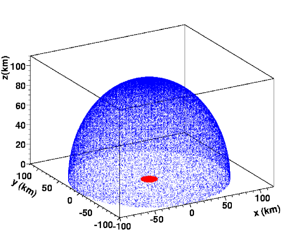
Figure 5.1: The spatial distribution of neutrino source locations isotropic over a positive hemispherical shell centred on the instrumented volume. Surrounding the instrumented volume is the cylindrical can. The radius of the shell is somewhat arbitrary as long as the shell itself encompasses the can. In this plot it is $100$ km.

The origin of the coordinate system that is employed in this simulation is defined to be at the centre of the instrumented volume at a depth of $2000$ m in a sea of depth $4000$ m. A conventional right-handed set of axes is fixed thus, with the $z$-axis running vertically and the $xy$-plane defining the horizontal. This coordinate system is illustrated in Figure 5.2. Typically $1000$ hydrophones are placed, at random, in a volume of one kilometre cubed, centred at the origin.

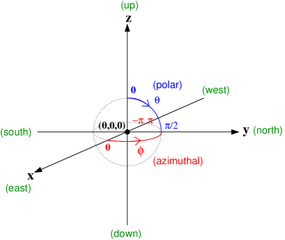
Figure 5.2: Coordinate system employed in the hydrophone array sensitivity estimation program.

5.4 Event Reconstruction

Signal arrival times are used to resolve interaction vertices. The formula for vertex reconstruction of sound rays that have undergone refraction is different from the formula that is used for rays that have linear trajectories.

5.4.1 Vertex location with linear rays

In a homogeneous medium the velocity of sound $c$ is constant. Point source location from differences in signal arrival times is well documented and has been implemented by the RICE [55], SAUND [67], Erlangen [69] and ACoRNE groups. The standard formalism is described below.

A receiver at location $\vec{r}_{i}$, hears a signal at time $t_{i}$, from a source at location $\vec{v}$, originating at time $t_{0}$, according to the following equation

$$|\vec{v}-\vec{r}_{i}|^{2}=c^{2}(t_{i}-t_{0})^{2}$$ (5.2)

Expanding the bracketed terms and solving for $\vec{v}$ gives:

$$v^{2}+r_{i}^{2}-2\vec{v}\cdot\vec{r}_{i} = c^{2}(t_{i}-t_{0})^{2}$$

$$(r_{i}^{2}-r_{j}^{2})-c^{2}[(t_{i}-t_{0})^{2}-(t_{j}-t_{0})^{2}] = 2\vec{v}\cdot(\vec{r}_{i}-\vec{r}_{j})$$

$$(r_{i}^{2}-r_{j}^{2})-c^{2}[t_{i}^{2}-t_{j}^{2}-2t_{0}(t_{i}-t_{j})] = 2\vec{v}\cdot(\vec{r}_{i}-\vec{r}_{j})$$

$$(r_{i}^{2}-r_{j}^{2})-c^{2}[t_{i}^{2}-t_{j}^{2}]+2c^{2}t_{0}(t_{i}-t_{j}) = 2\vec{v}\cdot(\vec{r}_{i}-\vec{r}_{j})$$

which can be expressed in the form of a matrix equation:

$$\overrightarrow{\mathbf{R}}+t_{0}\overrightarrow{\mathbf{T}}=\mathbf{M}\vec{v}$$ (5.3)

where, in the limiting case of four receivers:

$$\overrightarrow{\mathbf{R}} = {r_{i}^{2}-r_{j}^{2}-c^{2}(t_{i}^{2}-t_{j}^{2})}\quad(i,j=1,2;1,3;1,4)$$

$$\overrightarrow{\mathbf{T}} = {2c^{2}(t_{i}-t_{j})}\quad\qquad\qquad(i,j=1,2;1,3;1,4)$$

$$\mathbf{M} = 2\left(\begin{array}[]{ccc}dx_{12}&dy_{12}&dz_{12}\\ dx_{13}&dy_{13}&dz_{13}\\ dx_{14}&dy_{14}&dz_{14}\\ \end{array}\right)$$

(Here, the receiver with index $1$ is taken as the reference receiver, $dx,dy,dz$ are the difference in $x,y$ and $z$ coordinates respectively, between this receiver and the other receivers that detect a signal). Therefore:

$$\vec{v} = \mathbf{M}^{-1}(\overrightarrow{\mathbf{R}}+t_{0}\overrightarrow{\mathbf{T}})$$

$$= \mathbf{M}^{-1}\overrightarrow{\mathbf{R}}+t_{0}\mathbf{M}^{-1}\overrightarrow{\mathbf{T}}$$

One defines:

$$\overrightarrow{\mathbf{P}} = \mathbf{M}^{-1}\overrightarrow{\mathbf{R}}$$ (5.5)

$$\overrightarrow{\mathbf{Q}} = \mathbf{M}^{-1}\overrightarrow{\mathbf{T}}$$ (5.6)

then:

$$\vec{v}=\overrightarrow{\mathbf{P}}+t_{0}\overrightarrow{\mathbf{Q}}$$ (5.7)

The minimum number of receivers required for vertex reconstruction to be possible is four. If there are $n$ receivers the system becomes over constrained and matrix $\mathbf{M}$ becomes a $3\times(n-1)$ matrix. Because $\mathbf{M}$ is no longer symmetric it must be inverted using singular value decomposition (SVD). For an $(m\times n)$ matrix $\mathbf{A}$ with $m\geq n$, the singular value decomposition is given by:

$$\mathbf{A}=\mathbf{U\,L\,V}^{T}$$

where $\mathbf{U}$ and $\mathbf{V}$ are orthogonal $m\times m$ and $n\times n$ matrices containing the column and row eigenvectors respectively. $\mathbf{L}$ is an $m\times n$ matrix containing the eigenvalues in increasing order. The inverse of $\mathbf{A}$ is therefore given by:

$$\mathbf{A}^{-1}=\mathbf{V\,L}^{-1}\,\mathbf{U}^{T}$$

Since $\overrightarrow{\mathbf{P}}$ and $\overrightarrow{\mathbf{Q}}$ are known, it only remains to find $t_{0}$. This is done by solving the propagation time equation for any receiver amongst the four:

$$|\vec{v}-\vec{r}_{i}|^{2}=c^{2}(t_{i}-t_{0})^{2}=|\overrightarrow{\mathbf{P}}+t_{0}\overrightarrow{\mathbf{Q}}-\vec{r}_{i}|^{2}$$ (5.8)

which is simply a quadratic in $t_{0}$:

$$c^{2}t_{i}^{2}+c^{2}t_{0}^{2}-2c^{2}t_{i}t_{0}=\mathbf{P}^{2}+t_{0}^{2}\mathbf{Q}^{2}+r_{i}^{2}+2t_{0}\overrightarrow{\mathbf{P}}\cdot\overrightarrow{\mathbf{Q}}-2\overrightarrow{\mathbf{P}}\cdot\vec{r}_{i}-2t_{0}\overrightarrow{\mathbf{Q}}\cdot\vec{r}_{i}$$ (5.9)

rearranging for $t_{0}$ gives:

$$(c^{2}-\mathbf{Q}^{2})t_{0}^{2}+(2\overrightarrow{\mathbf{Q}}\cdot\vec{r}_{i}-2\overrightarrow{\mathbf{P}}\cdot\overrightarrow{\mathbf{Q}}-2c^{2}t_{i})t_{0}-(\mathbf{P}^{2}+r_{i}^{2}-2\overrightarrow{\mathbf{P}}\cdot\vec{r}_{i}-c^{2}t_{i}^{2})=0$$ (5.10)

Both roots to Equation 5.9 are potentially viable. The correct root is sought by minimising the following chi-squared:

$$\chi^{2}=\sum_{i=0}^{N_{\textrm{receivers}}}(t_{i}-t_{r})^{2}$$ (5.11)

where as before $t_{i}$ is the arrival time of the signal at the receiver located at $\vec{r}_{i}$, and the reconstructed time $t_{r}$ is given, in terms of the signal emission time $t_{\pm s}$ and vertex location $\vec{v}_{\pm}$, from the positive and negative solutions, by:

$$t_{r}=t_{\pm s}+\frac{(\vec{r}_{i}-\vec{v}_{\pm})}{c}$$

which yields the correct root $99.9\%$ of the time. Interestingly, simply invoking causality is not sufficient since in many cases both roots are allowed; the exact number of causal and non-causal roots is dependent on the geometry of the detector and the can. The vertex resolution of a one thousand hydrophone array, of one cubic kilometre instrumented volume in the case of a constant sound velocity, is plotted in Figure 3.

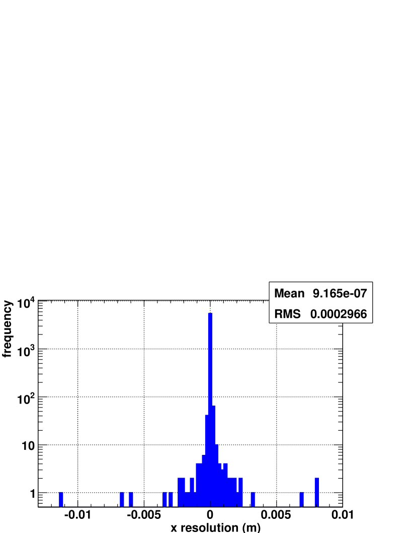
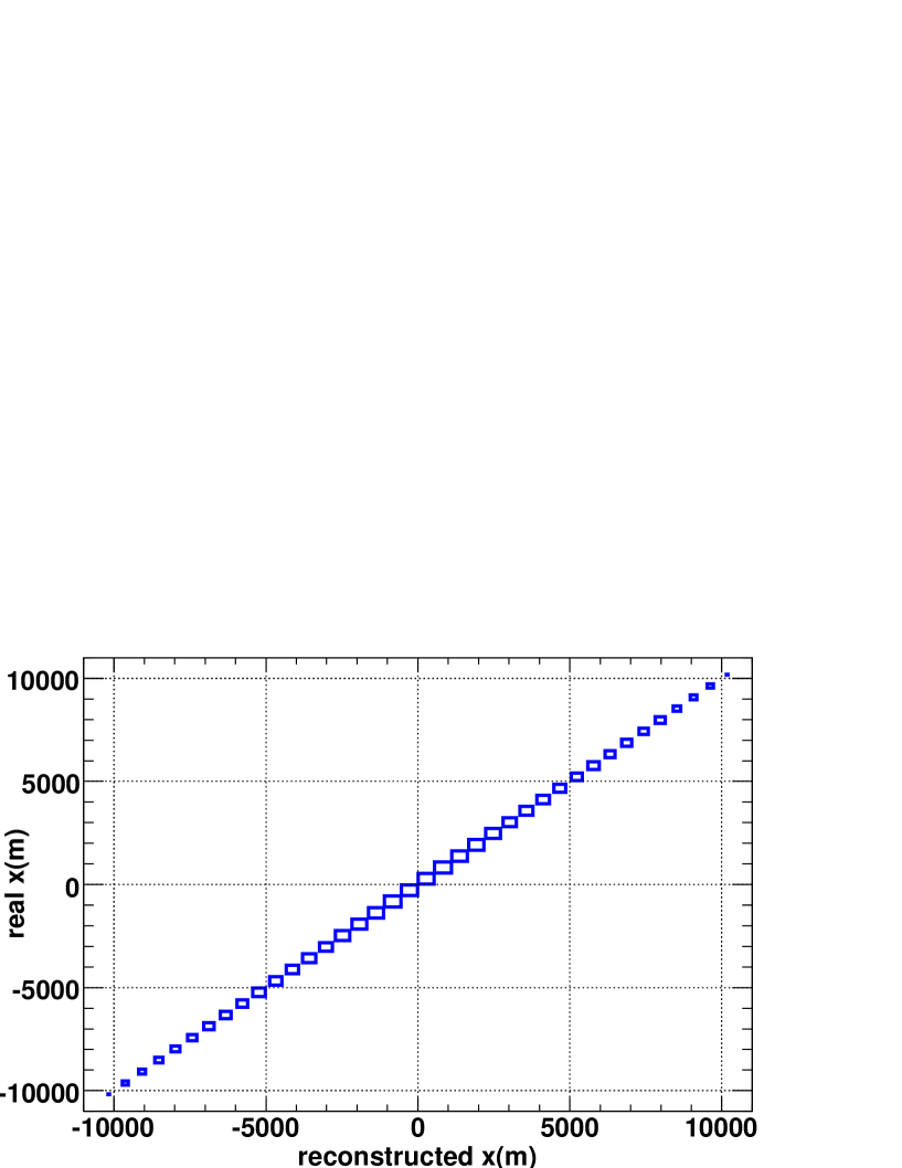
Figure 5.3: The resolution of the vertex $x$-coordinate, in the case of a constant sound velocity and no smearing on the hydrophone location, has a mean value consistent with zero and a standard deviationof less than $1$ mm.

Now, given the interaction vertex, and a set of receiver signals confined to a plane perpendicular to the direction of the neutrino, all one has to do to resolve the cosmic source of the neutrino is point back through the vertex with a vector normal to the pancake plane. The neutrino pointing vector has been reconstructed in two ways: firstly by taking the normal to the plane defined by the vertex and the two most energetic receivers in the pancake, as illustrated in Figure 5.4; secondly by taking the cross product of two vectors orthogonal to each other and the cascade direction, as plotted directly from the simulation in Figure 5.4.

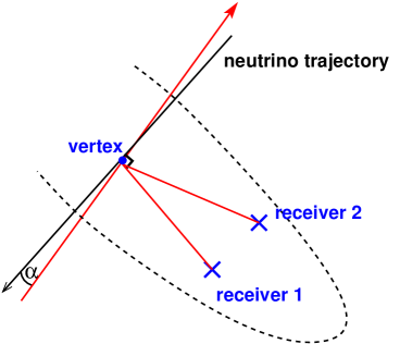
Figure 5.4: The vector normal to the plane defined by a pair of hydrophones lying in the acoustic pancake and the reconstructed vertex points back along the axis of the hadronic cascade. Hence this vector is collinear with the trajectory of the incident neutrino. The pointing resolution is defined by the angle $\alpha$ between the pointing vector and the incoming neutrino trajectory.

The procedure, subsequently called the “Top2” algorithm, for determining these vectors is as follows:

1. calculate the centre of mass of the system of hit receivers - this lies in the plane of the pancake; then, translate the coordinate system such that the origin is at the centre of mass.

2. Define a vector $\vec{v}_{1}$ that points from the centre of mass to the vertex.

3. Rotate the coordinate system such that $\vec{v}_{1}$ is aligned along (say) the $x$-axis, then collapse the system into $2D$ by discarding the $x$-coordinates.

4. Perform a least squares fit to the hit receivers in $yz$-plane, because the centre of gravity is at the origin, the intercept of this line will be at zero, define a second vector $\vec{v}_{2}$ in the direction of this line.

5. Rotate the system back - vectors $\vec{v}_{1}$ and $\vec{v}_{2}$ are orthogonal to each other, the neutrino pointing vector is simply $\vec{v}_{1}\times\vec{v}_{2}$.

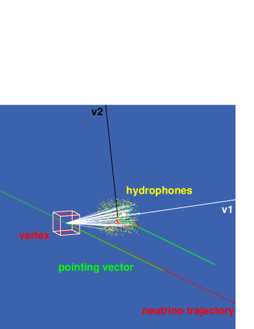
Figure 5.5: Output from the simulation displaying vectors $\vec{v}_{1}$ and $\vec{v}_{2}$ and the resultant pointing vector as described in the text.

The pointing resolution is defined as the angle $\alpha$ between the real neutrino trajectory and the reconstructed pointing vector. A comparison of the resolution from both methods discussed above is plotted in Figure 5.6, a mean pointing resolution of $6.9$ ^∘ is obtained from the Top2 algorithm and $12.0$ ^∘ from the collapsed mean algorithm, in the absence of refraction, for an array of $1000$ hydrophones distributed at random in a volume of one cubic kilometre.

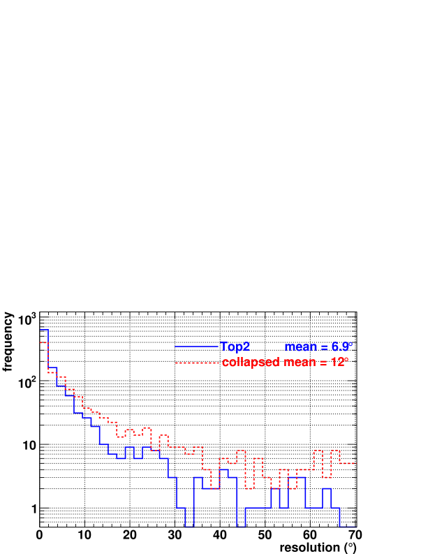
Figure 5.6: The pointing resolution of both reconstruction techniques for an array of one thousand hydrophones distributed randomly in a volume of one kilometre cubed and a can radius of $10$ km. The resolution is defined as the angle between the true neutrino trajectory and the reconstructed pointing vector.

5.4.2 Vertex location with curvilinear rays

If the velocity of sound is a function of depth, $c=c(z)$, then Equation 5.2 is no longer valid. Sound rays follow curved trajectories and the pancake becomes warped, this is illustrated in Figure 5.7. Unlike for constant sound velocity, there is no analytical solution to the event vertex $\vec{v}$ and the signal emission time $t_{0}$.

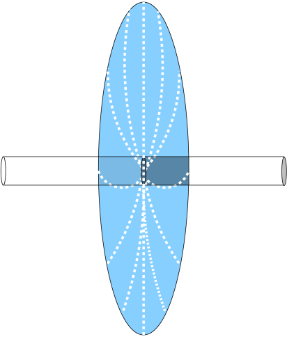
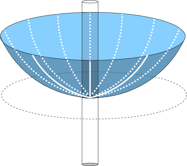
Figure 5.7: Schematic of the energy deposition. Refraction occurs only in the vertical plane; there are two extreme cases: that when the shower is horizontal (Left) and that when the shower is vertically inclined (Right). In the former case, there is no deformation of the pancake such that the radiation field is bent outside the plane orthogonal to the shower axis.

One now relies on iterative minimisation to interpolate towards event vertices in the presence of refraction. This concept has been employed elsewhere by the RICE [55] and SAUND [67] collaborations to enable reconstruction of vertices in the data from their respective experiments. For a given set of hits on a sensor array one can minimise the following metric:

$$\mathbf{M}=\sum_{i=0}^{N_{\textrm{receivers}}}(t_{i}-t_{v})^{2}$$ (5.12)

where $t_{i}$ is the arrival time of the signal recorded by the receiver located at $\vec{r}_{i}$ and $t_{v}$ is the time it takes for a signal from a test location $\vec{v}$ to reach the same receiver. In references [55] and [67] minimisation begins from a location determined by analysis of precomputed look-up tables containing the sensor hit times for regularly spaced locations in the fiducial volume surrounding the detector. In this approach, the number of test locations, and hence computations, scales with the size of the fiducial volume under consideration. When volumes of a hundred or so cubic kilometres are being dealt with the process becomes inefficient, taking several minutes per event (depending on can size and lattice density). Instead, an estimate of the vertex location is sought from which the minimisation procedure can begin.

The equations for point source location in a homogeneous medium, from signal arrival times, can be used to approximate the location of a point source in an inhomogeneous medium. Starting with Equation 5.3, where, in the limiting case of four receivers:

$$\overrightarrow{\mathbf{R}} = {r_{i}^{2}-r_{j}^{2}-c^{2}(t_{i}^{2}-t_{j}^{2})}\quad(i,j=1,2;1,3;1,4)$$

$$\overrightarrow{\mathbf{T}} = {2c^{2}(t_{i}-t_{j})}\quad\qquad\qquad(i,j=1,2;1,3;1,4)$$

$$\mathbf{M} = 2\left(\begin{array}[]{ccc}dx_{12}&dy_{12}&dz_{12}\\ dx_{13}&dy_{13}&dz_{13}\\ dx_{14}&dy_{14}&dz_{14}\\ \end{array}\right)$$

Again, the receiver with index $1$ is taken as the reference receiver, $dx,dy,dz$ are the difference in $x,y$ and $z$ coordinates respectively, between this receiver and the other receivers that detect a signal. Additionally $c=c(z)$, where $z$ is the mean depth of the four receivers and $\mathbf{M}$ is always a $3\times 3$ square matrix. Solving for the vertex $\vec{v}$ gives:

$$\vec{v}=\mathbf{M}^{-1}\overrightarrow{\mathbf{R}}+t_{0}\mathbf{M}^{-1}\overrightarrow{\mathbf{T}}$$

which is once more solved via the propagation time equation:

$$|\vec{v}-\vec{r}_{i}|^{2}=c^{2}(t_{i}-t_{0})^{2}=|\mathbf{M}^{-1}\overrightarrow{\mathbf{R}}+t_{0}\mathbf{M}^{-1}\overrightarrow{\mathbf{T}}-\vec{r}_{i}|^{2}$$

The mean vertex $\overline{\vec{v}}$ from $N_{q}$ quadruplets of receiver signals is thus calculated as:

$$\overline{\vec{v}}=\frac{1}{N_{q}}\sum_{i=0}^{i=(N_{q})}\vec{v}_{i}$$ (5.14)

There are:

$${}_{N}C^{4}=\frac{N!}{(N-4)!4!}$$ (5.15)

unique receiver quadruplets from $N$ receiver signals. This number rapidly diverges as $N$ increases; for example, there are $230300$ possible four-receiver combinations of $50$ receivers. Furthermore calculation of the unique permutations is in itself computationally intensive. As such a “reduced mean” with fewer elements is desired. Three “reduced mean vertices” have been considered. The first is the mean vertex from each receiver and its three spatial-nearest-neighbours; the second is the mean vertex from each receiver and its three temporal-nearest-neighbours; and the third is the mean vertex from each receiver and its three pressural-nearest-neighbours. In each case there are only $N-3$ contributions to the mean, so for $50$ receivers there are only $46$ permutations compared to the $230300$ above. All three methods rely on Equation 5.11 to solve for the vertex, utilising the sound velocity at the mean depth of a given receiver quadruplet. Now, neither root of the quadratic is in fact a unique solution to the propagation time equation (Equation 5.9) since we have substituted a linearly variable sound velocity in place of a constant sound velocity. As such there is an inherent instability in the estimation method, however, an estimate of the mean is found nonetheless. Calculation of estimated vertices takes less than one second per event on a standard $2$ GHz processor with $512$ MB of RAM.

The comparative vertex $x$-coordinate resolution from the three reduced mean vertices is plotted in Figure 5.8, indicating that the temporal-nearest-neighbours gives the best estimate of the vertex. The $x$ resolution of the temporal mean with respect to the unreduced mean is subsequently plotted in Figure 5.9, confirming that the vertex estimate from this method is not only a computationally less intensive than taking the mean vertex from all receiver combinations but more accurate. The standard deviation on the shower time, $\sigma_{t}$, for each of the reduced mean vertices is displayed in Table 5.1; here it can be seen why the reduced temporal mean gives the best performance, showing the smallest intrinsic error on the shower time as returned by Equations 5.9 and 5.11.

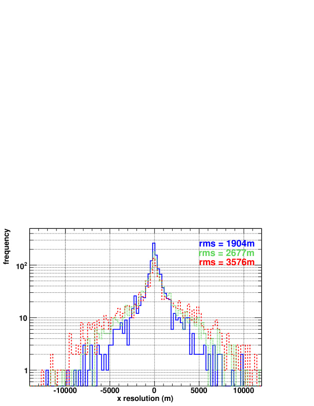
Figure 5.8: The resolution of the reconstructed vertex $x$-coordinate. The solid curve represents the temporal mean with $\sigma=1904$ m; the dotted curve is the pressural mean with $\sigma=2677$ m; and, the dashed curve is the spatial mean with $\sigma=3576$ m. No smearing on the hydrophone locations was included and an array of $200$ hydrophones distributed at random in a volume of one kilometre cubed was used. $10,000$ neutrinos were generated in a can of radius $10$ km.

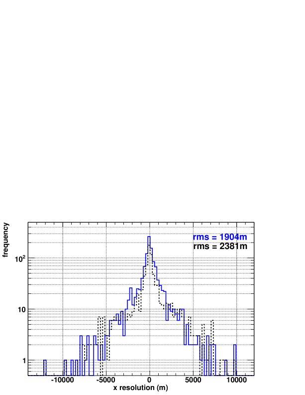
Figure 5.9: The resolution of the reconstructed vertex $x$-coordinate. The solid curve represents the temporal mean with $\sigma=1904$ m and the dashed curve is the unreduced mean with $\sigma=2381$ m.

Minimisation of Equation 5.12 begins from the reduced temporal mean vertex and is performed by MINUIT [84], the de facto High Energy Physics minimisation package. A comparison of the vertex resolution of the unreduced mean, the reduced temporal mean and the vertex returned by MINUIT is plotted in Figure 5.10.

Figure 5.10: The resolution of the reconstructed vertex $x$-coordinate. The solid curve represents the temporal mean with $\sigma=1904$ m and the dashed curve is the minimised $x$ resolution with $\sigma=1259$ m.

Reduced Mean	$\sigma_{t}$ (s)
temporal	2.68
spatial	2.98
pressural	3.04

Table 5.1: Standard deviations of the shower times returned by Equations 5.9 and 5.11 for each of the reduced mean methods in a can of radius $10$ km.

Vertex minimisation for the same $200$ hydrophones as for each of the estimated vertices is evaluated in Table 5.2. Eighty-seven percent of temporal minimised vertices are found to within $1000$ m of the true vertex compared to $68\%$ of estimated vertices; furthermore, $30\%$ of minimised vertices are reconstructed to within $0.1$ m of the true vertex compared to $1\%$ or less of estimated vertices. Naturally different array densities will offer different reconstruction performance and this will be discussed further in Section 5.6. Furthermore increasing the radius of the fiducial volume beyond $10$ km will make the effects of refraction more pronounced.

A note on MINUIT performance

The performance of MINUIT is not only sensitive to the starting parameters but the topology of the $\chi^{2}$ hypersurface and has not been optimised in this study. The minimisation procedure begins with some estimate of the true vertex as returned by the temporal-nearest-neighbour vertexing algorithm described previously. Additionally one must specify an estimate of the error on the associated parameters, namely the $x$, $y$ and $z$ coordinates of the estimated vertex. Furthermore one must decide whether to constrain the values that $x$, $y$ and $z$ can take or whether to leave them unconstrained. In this study the vertex coordinates were constrained to be within the fiducial volume, i.e. the can. This was decided to be so because an unconstrained fit can lead to test locations well beyond the fiducial volume, resulting in ray traces over thousands of kilometres. This is problematic because the number of iterations possible in the ray trace calculation is limited by the amount of physical memory in the computer on which the simulation is running. One can arbitrarily reduce the number of iterations made but this reduces the number of straight line segments used to approximate the circular ray path and thus causes it to appear more and more like a straight line therefore reducing the accuracy of the operation. An expression for the error on the estimated vertex on an event by event basis should improve the minimisation procedure; however, for the purpose of this study the error in $x$ and $y$ was set at one can radius and the error in $z$ was set at one can height for every event. Additionally the vertex reconstruction problem in the presence of refraction is non-linear and as such MINUIT is not guaranteed to successfully converge on the best solution.

		Temporal		Spatial		Pressural
	Res. $<\pm$	estimated	minimised	estimated	minimised	estimated	minimised
	$1000$ m	$68\%$	$87\%$	$43\%$	$81\%$	$64\%$	$84\%$
	$100$ m	$19\%$	$64\%$	$10\%$	$59\%$	$27\%$	$63\%$
	$10$ m	$3\%$	$49\%$	$1.8\%$	$48\%$	$7\%$	$48\%$
	$1$ m	$0.4\%$	$39\%$	$0.3\%$	$34\%$	$2\%$	$39\%$
	$0.1$ m	$0\%$	$30\%$	$0.08\%$	$26\%$	$1\%$	$29\%$
	$0.01$ m	$0\%$	$14\%$	$0\%$	$13\%$	$0.7\%$	$13\%$

Table 5.2: Minimised vertex performance. The resolution is defined as $x_{recon}-x_{real}$ where $x_{recon}$ and $x_{real}$ are the reconstructed and real vertex $x$-coordinates respectively. Minimisation beginning from the temporal mean vertex can be seen to provide the best performance. Here the can radius is $10$ km.

5.5 The Effective Volume

The effective volume $V_{eff}$ of a simulated array is defined as:

$$V_{eff}=\frac{N_{det}}{N_{gen}}\times V_{gen}$$ (5.16)

where $N_{det}$ and $N_{gen}$ are the number of events that are detected and the number of events that are generated respectively, and $V_{gen}$ is the volume in which events are generated. The behaviour of Equation 5.16 is such that by increasing the volume $V_{gen}$ in which event vertices are generated, $V_{eff}$ will increase proportionally, however this is offset by a reduction in the number of detections, particularly at lower energy and in essence therefore raises the threshold. $V_{gen}$ should certainly extend beyond the instrumented volume and in practice one usually fixes the size of $V_{gen}$ with the maximum range for source detection, remembering that beyond $24$ km parts of the sea are geometrically inaccessible to sound rays subtending the array (see Figure 4.9 in Section 4.3). Running the simulation with no pressure threshold and a can radius greater than $48$ km determines the extent to which events can be detected as constrained by geometry only. The range of those events that produce a reconstructable vertex is plotted in Figure 5.11. This range determines the radius of the volume $V_{gen}$ when calculating the effective volume, $V_{eff}$.

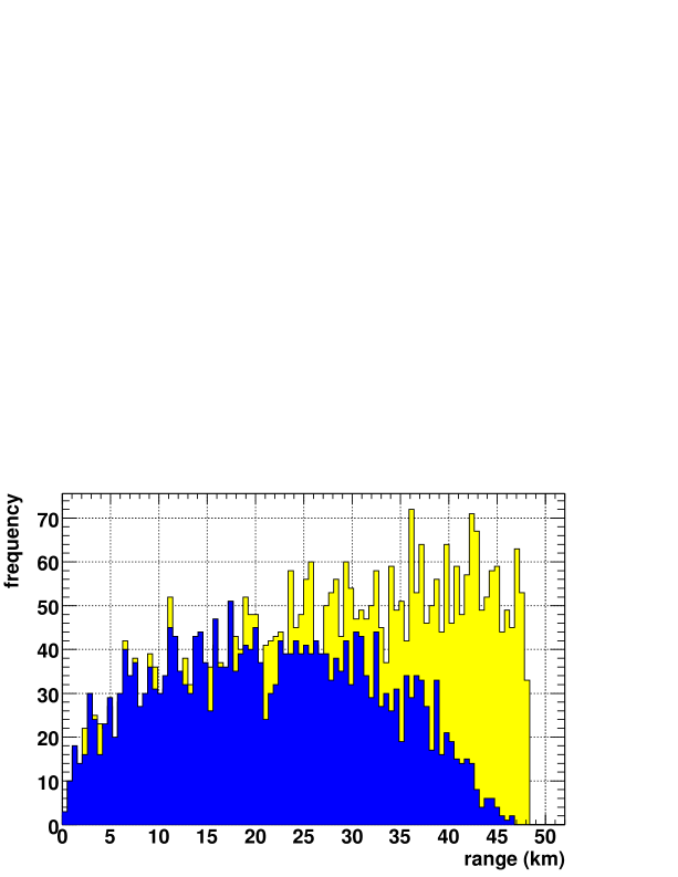
Figure 5.11: Range of events accessible due to the limitations imposed by refraction. The lighter histogram corresponds to the range of events detected if refraction is neglected and shows a continuous acceptance up to $48$ km. The darker histogram is the range of detected events in consideration of refraction. Beyond $24$ km the acceptance reduces until no events are detected at a range just below $48$ km.

Given an expression for the effective volume, with a $48$ km can radius it is possible to test the effect of different array densities. An optimum number of hydrophones is sought, that is, the minimum number of sensors required above which there is no significant improvement in the effective volume. This relationship is plotted in Figure 5.12. Above a density of $400$ hydrophones per cubic kilometre the gain in effective volume is small, especially above $10^{12}$ GeV. At lower energies sensor density is of more importance; at least $800$ hydrophones per cubic kilometre are required for an optimal $v_{eff}$. The matter of hydrophone density still requires further discussion with respect to the resolving power of a given array.

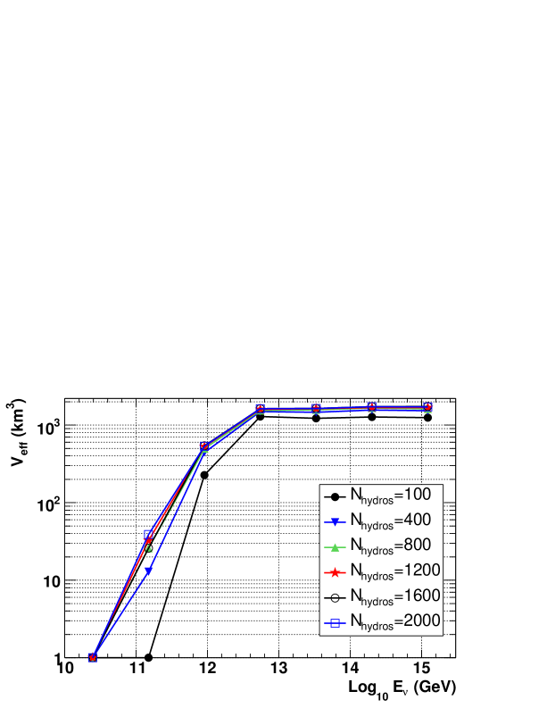
Figure 5.12: Effective volume as a function of hydrophone density for cubic kilometre arrays.

5.6 Optimal Hydrophone Density for Reconstruction in the Presence of Refraction

The sensitivity of a hypothetical detector relies on its ability to reconstruct the vertex of a given event. However if such a detector is to be used as a “telescope” for the purpose of Neutrino Astronomy, then it must also provide information on the trajectory and energy of a neutrino. One may therefore pose the following question: “what is the optimal hydrophone density required to provide the best vertex and pointing resolution, via the reconstruction algorithms introduced thus far?” Typically one thousand hydrophones have been considered in a volume of one kilometre cubed. From Section 5.5 a minimum number of sensors has been found for which the effective volume of an array is maximal. An optimum sensor density for vertexing and pointing accuracy is now desired. The standard deviation on the vertex $x$, $y$ and $z$ coordinates as a function of hydrophone density and the number of reconstructions within $10$ cm of the actual vertex location are plotted in Figure 5.13.

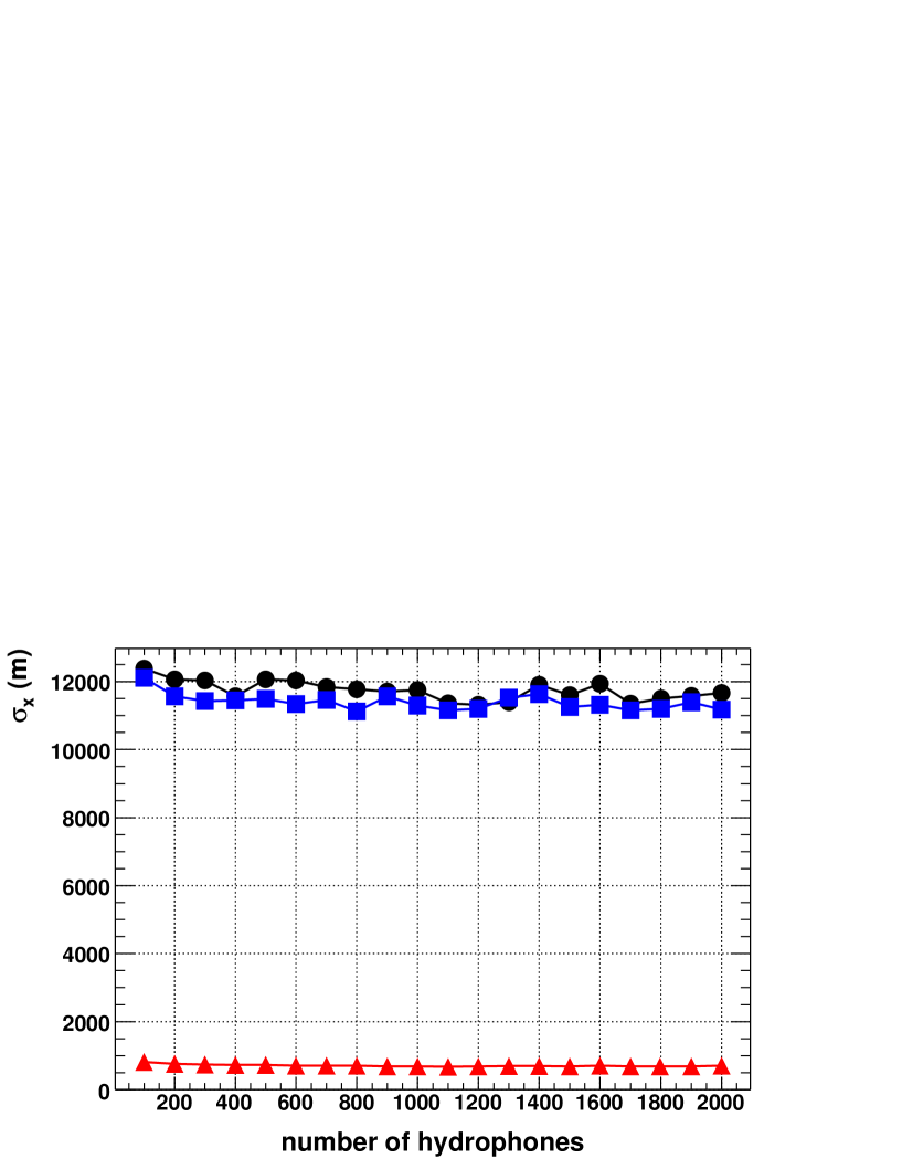
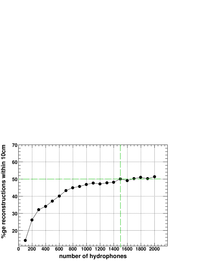
Figure 5.13: Resolution (Left) and accuracy (Right) of vertexing as a function of the number of hydrophones. Resolution in $x$ ($\bullet$ marker) and $y$ ($\blacksquare$ marker) plateaus beyond a hydrophone density of a $300$ per cubic kilometre whereas the number of reconstructions up to a given accuracy continues to improve up to a hydrophone density of $1500$ per cubic kilometre. Because the can is much larger radially ($48$ km) than it is in height ($4$ km) the $z$-coordinate ($\blacktriangle$ marker) resolution is much better than in $x$ and $y$.

The pointing reconstruction as a function of hydrophone density is evaluated in Figure 5.14.

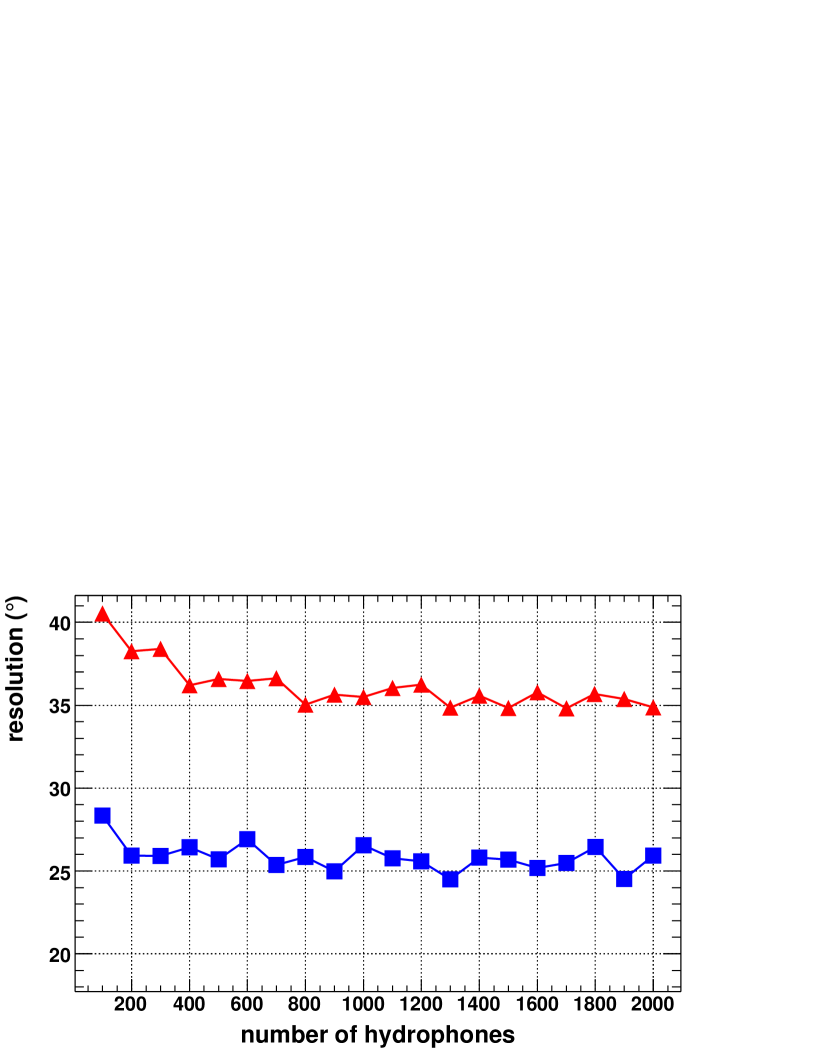
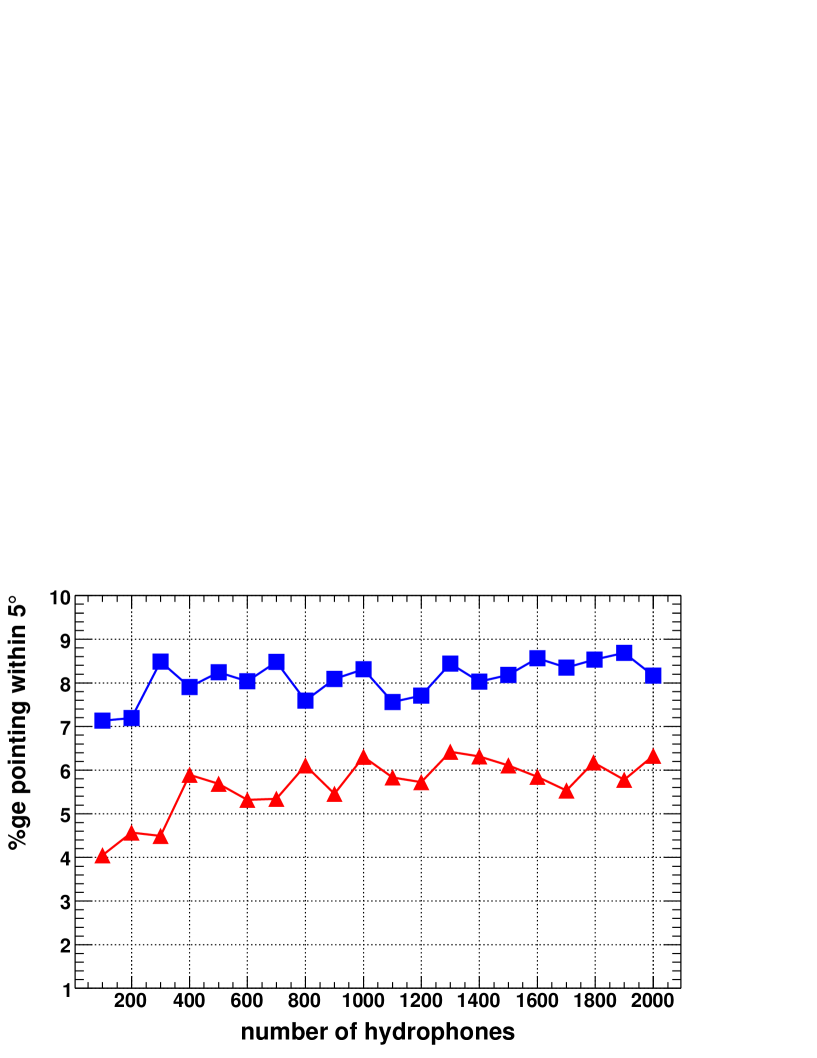
Figure 5.14: Top2 ($\blacksquare$ marker) and Collapsed ($\blacktriangle$ marker) pointing resolution (Left) and accuracy (Right). In each case there is little improvement (within fluctuations) from beyond $600$ hydrophones per cubic kilometre.

5.7 The Effect of Uncertainty in Hydrophone Locations

The ANTARES [19] neutrino telescope utilises a High Frequency Long Base Line (HFLB) acoustic positioning system, operating at $40-60$ kHz over a base of $300\times 300$ m, combined with local tilt-meter-compass sensors to obtain the location of its sensor elements in the depths of the Mediterranean Sea. The system provides spatial positioning to an accuracy of $0.1$ m. One may therefore assume that any future undersea detector array will have at least comparable performance. The effect of smearing the hydrophone locations by a Gaussian distribution with width $\sigma_{h}=0.1$ m on the standard deviation of the vertex $x$-coordinate ($\sigma_{x}$) and the Top2 pointing vector ($\sigma_{\mathrm{Top2}}$) is summarised in Table 5.3.

	Vertexing		Pointing
$\sigma_{h}$ (m)	$\sigma_{x}$ (m)	$\sigma_{x}<0.1$ m	$\sigma_{\mathrm{Top2}}$ (∘)	$\sigma_{\mathrm{Top2}}<5$ ∘
$0.0$	$11230$	$47.6\%$	$28.0$	$8.89\%$
$0.1$	$11800$	$47.5\%$	$28.6$	$8.60\%$

Table 5.3: The effect of a $0.1$ m hydrophone location uncertainty on reconstruction performance of a $1000$ hydrophone, $1$ km³ array in a can of radius $48$ km.

5.8 Reconstruction of the Neutrino Energy

As previously stated, an estimate of the energy of an interacting neutrino is required if one is to use a hydrophone array for neutrino astronomy. To be able to identify a source in the sky is one thing, but to understand the processes occurring therein some kind of calorimetry is necessary. A simple method was tested for determining the energy resolution. The following $\chi^{2}$ was evaluated:

$$\chi^{2}=\sum_{h=1}^{N_{\mathrm{hydros}}}P_{h}-P_{e}$$ (5.17)

where $N_{\mathrm{hydros}}$ is the number of hydrophones in the array, $P_{h}$ is the pressure recorded on each hit hydrophone and $P_{e}$ is the pressure expected at each phone. The pressure expected at each phone is a function of the reconstructed vertex location, the angle out of the plane of the pancake and the incoming neutrino energy. $\chi^{2}$ is calculated for a range of energies and the energy at which it is a minimum should then correspond to the energy of the incoming neutrino.

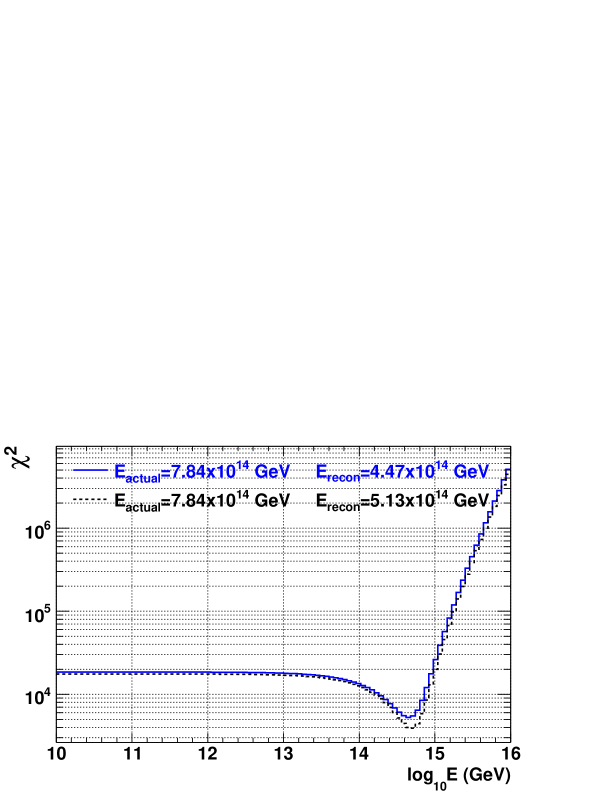
Figure 5.15: Plot of $\chi^{2}$ as described by equation 5.17 for one event with successful vertex reconstruction with (solid curve) and without (dashed curve) refraction. In each case the energy is reconstructed below the true value.

As can be seen from the plot in Figure 5.15 the $\chi^{2}$ minimisation has yielded a result that is below the actual neutrino energy; however, this is easily explained. Here the expected energies were calculated merely as function of the distance of the resolved vertex without considering the attenuation due to being outside the plane of the pancake. So, the expected pulses on those phones outside the pancake plane is over-estimated, the true neutrino energy would have to be slightly larger in reality to produce these signals. We can see this effect more easily in Figure 5.16 which displays $log_{10}E_{\mathrm{recon}}$ on the horizontal axis and $log_{10}E_{\mathrm{actual}}$ on the vertical axis, for over a thousand events. Superimposed on the plot is the line $y=x$ to aid the observation of the systematic shift of the $E_{\mathrm{recon}}$ towards lower energy. The mean reconstructed energy is $(61\pm 17)\%$ of the actual energy in the presence of refraction and $(63\pm 12)\%$ without. Naturally one can assume that adding the effects of angular attenuation to the $\chi^{2}$ calculation will improve the reconstruction; however this has not been undertaken in this work. Instead, to give an estimate of the potential energy reconstruction performance $E_{\mathrm{recon}}$ has been multiplied by a scale factor in order to systematically shift values to higher energy, this can be seen plotted in Figure 5.16. The resulting energy resolution is plotted in Figure 5.17.

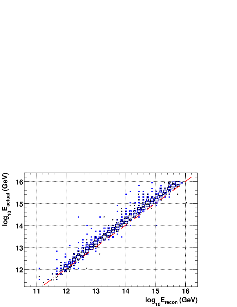
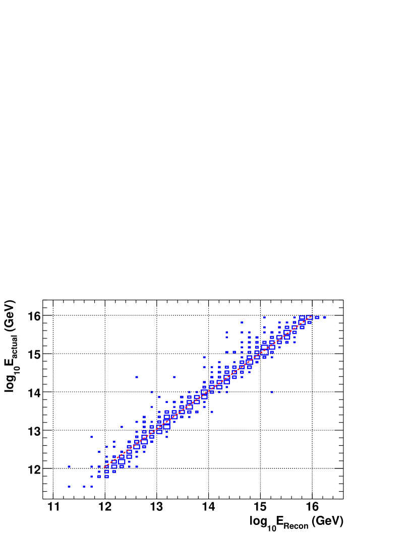
Figure 5.16: (Left) The distribution of $E_{\mathrm{recon}}$ v.s.$E_{\mathrm{actual}}$,it is offset from the dashed line $E_{\mathrm{recon}}=E_{\mathrm{actual}}$ due to systematic underestimation of the neutrino energy. (Right) The shifted distribution of $E_{\mathrm{recon}}$ v.s.$E_{\mathrm{actual}}$ compensating for the underestimation of the neutrino energy. Both plots include the effects of refraction.

Up until this point it has been assumed that a constant $25\%$ of the energy of the incident neutrino is imparted upon the resulting hadronic cascade which in turn generates the thermoacoustic pressure wave detected a given hydrophone array. As discussed in Section 3.2 the proportion of the neutrino energy liberated by the cascade can in fact fluctuate from $0-100\%$. Including the effects of a non-constant Bjorken-$y$ by sampling from the distribution plotted in Figure 3.3(b) value reduces the effectiveness of the energy reconstruction (by a factor orders of magnitude greater than the underestimation error); the resulting energy resolution is plotted in Figure 5.17.

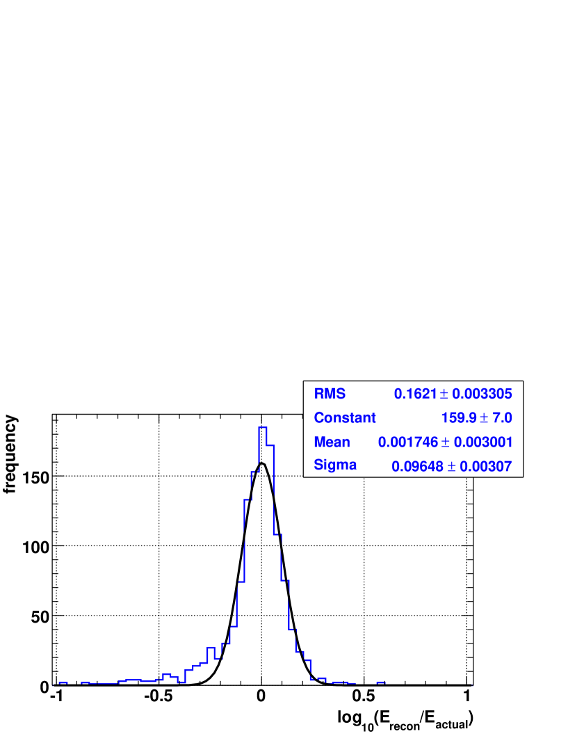
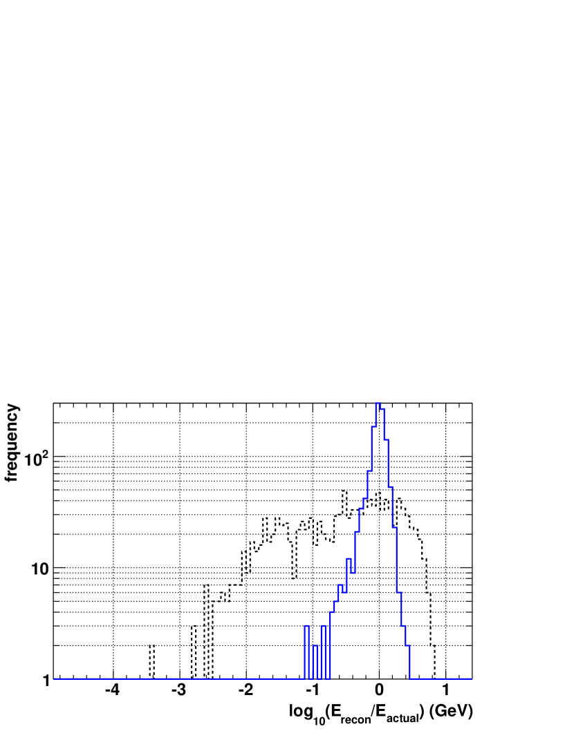
Figure 5.17: (Left) Potential energy resolution with $\sigma_{\log_{10}E}\sim 0.1$, assuming a constant Bjorken-$y$ of $0.25$. (Right) Energy resolution with $\sigma_{\log_{10}E}\sim 0.8$, smeared by a non-constant Bjorken-$y$ (dashed) on top of the unsmeared energy resolution (solid). Both plots include compensation for systematic underestimation of the neutrino energy and include the effects of refraction.

5.9 The Sensitivity Calculation and Predicted Results

The simulations described thus far determine the ability of a given hypothetical array of hydrophones to detect UHE neutrinos across a range of energies. For a given energy, it is therefore possible to place an upper limit on the neutrino flux, assuming that no events are detected within a certain time window. The following calculation is based on the formalism laid out in reference [50]. The principal equation is:

$$\Phi(E)=\frac{S_{\mathrm{up}}}{E\times\lambda(E)}$$ (5.18)

• $\Phi(E)$ is the limit on the differential flux $[dN_{\nu}/dEdAd\Omega dt]$ in units of
  GeV^-1cm^-2 sr^-1 s^-1.

• $S_{\mathrm{up}}$ is the upper limit on the number of detected events that one places. Assuming that no events are seen, then 95% confidence level upper limits correspond to setting $S_{\mathrm{up}}=3.0$  (or $2.3$ for 90% confidence level) in the absence of background [85].

• $\lambda(E)$ is the number of events that we would detect if a unit differential flux were incident on our detector at a unique energy $E$, for time $T$. It can therefore be written as:

  $$\lambda(E)=\sigma_{\nu N}(E)\times\rho\times N_{\mathrm{A}}\times V\times 2\pi\times f_{MC}(E)\times T$$ (5.19)

  where:

  • $\sigma_{\nu N}(E)$ is the neutrino-nucleon cross section at energy $E$. This is an extrapolated result (see Appendix A.1).

  • $\rho$ is the density of water.

  • $N_{\mathrm{A}}$ is Avogadro’s number.

  • $V$ is the fiducial volume (i.e. the can) where $V=\pi\times(R_{\mathrm{can}})^{2}\times H_{\mathrm{can}}$.

  • $T$ is the exposure time in seconds

  • $f_{MC}(E)$ is the fraction of Monte Carlo events generated at energy $E$ that are detected (and reconstructed).

The sensitivity of an array of $1000$ hydrophones, distributed at random in a volume of one cubic kilometre, is plotted in Figure 5.18 (labelled 1yr-35mPa-1000), the pressure threshold is $35$ mPa and the period of operation one year. Also shown is the sensitivity of $1500$ km³ array, with $100$ hydrophones per cubic kilometre operating at a pressure threshold of $5$ mPa for $5$ years (labelled 5yr-5mPa-1500). This is an indicator of the size and scale of an array required if one is to be sensitive to the cosmogenic neutrino flux (labelled GZK) resulting from the attenuation of UHECRs on the $2.7$ K CMB photons. The sensitivity curves for this study and the other experiments included on the plot represent a limit on the neutrino flux based on no neutrinos being detected within the period of operation. Also shown are the neutrino fluxes predicted by some theoretical models.

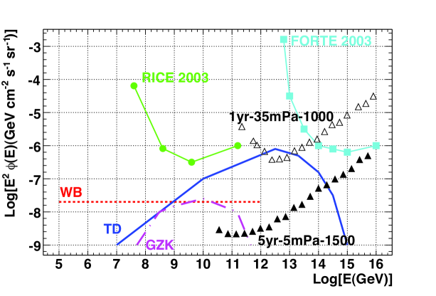
Figure 5.18: Predicted limits on the neutrino flux from this study ($\triangle$ and $\blacktriangle$), RICE ($\bullet$) and FORTE ($\blacksquare$). Also shown are those fluxes predicted by the Waxman-Bahcall (dotted), Topological Defect (solid) and GZK (dash-dotted) models from Figure 2.13.

5.10 Summary

The details of a simulation dedicated to calculating the ability of hypothetical large scale arrays of hydrophones to detect a flux of UHE neutrinos, has been reported. Through the use of ray tracing algorithms, the effects of refraction have been incorporated on an event by event basis on cubic kilometre scales, building on previous work ([80],[69]) which neglected or approximated refractive effects. The treatment of vertex reconstruction, which in a homogeneous medium can be solved analytically with almost perfect accuracy (see Figure 3), presents a non-linear problem, without an analytically determinable solution. Numerical computation of refracted vertices has subsequently been discussed, extending the work beyond that which incorporates pre-computed look-up tables ([55],[67]) which prove to be computationally expensive when looking to simulate arrays of thousands of cubic kilometres. Additionally the dependencies of effective volume, vertex resolution and pointing accuracy on hydrophone density have been investigated. A full study of array optimisation is required to maximise performance for all three effects in unison. Array performances have been translated into limits on the neutrino flux as a means of comparing the sensitivity of different instrumented volumes. In order to observe and successfully reconstruct a so-called GZK neutrino, it has been shown that hydrophone arrays encompassing volumes of several thousand cubic kilometres and operating at pressure thresholds of around $5$ mPa are required.

Chapter 6 First Data from Rona Underwater Acoustic Range

6.1 Introduction

The ACoRNE collaboration has access to the QinetiQ Underwater Acoustic Range at Rona in Northwest Scotland. This facility is operated and maintained by QinetiQ on behalf of the Ministry of Defence (MoD) and is used for the measurement of radiated acoustic signatures from Royal Navy ships and submarines in broad equivalence to the United States AUTEC array in the Bahamas as used by the SAUND collaboration. The array comprises eight wide band hydrophones distributed along Inner Sound - a $12$ km long strait separating the Inner Hebridean islands of Rassay and Rona from the Scottish mainland - with an average depth of $\sim 230$ m. Six of the hydrophones are located at mid-water on cables that are anchored at the lower end to the seabed and pulled taut by a buoy tethered at the upper end, one is anchored to the floor and the eighth is $30$ m from the bottom. The array extends over about one and a half kilometres and thus has a sound transit time of approximately one second. Since December $2005$ data acquisition has been underway. The first run constituted $15$ days of continuous readout at a sampling frequency of $140$ kHz and amounted to $2.8$ TB of raw information.

6.2 Data Acquisition

6.2.1 Recording the hydrophone signals

The eight Rona hydrophones are commercially available wide band sensors with a flat frequency response up to resonance at $50$ kHz. The ACoRNE data acquisition (DAQ) philosophy is to send all data to shore unfiltered and archive it for processing and analysis offline. Every ten minutes each of the Rona hydrophones produces a waveform audio format (WAV) file; the eight files are placed in a time-stamped directory and written immediately to an $8$ TB RAID disk array. In September $2006$ the DAQ was upgraded to incorporate an LT03 tape drive with mechanical loader and barcode reader. The WAV files are compressed using the Free Lossless Audio Compression (FLAC) codec and written onto $400$ GB LT03 tapes nightly and then removed from the RAID array. Compression via FLAC reduces the file size to approximately $45\%$ of its orginal size, with no loss of information. Because of the sensitive nature of the Rona facility remote access to these data is impossible; as such tapes are physically mailed to ACoRNE members by the operating staff. No filtering whatsoever has been introduced thus far, so prior to analysis the raw data remains intact.

The motivation for such a byte-intensive system is to enable the use of linear-phase digital filters. Unless the phase response of a recording system is linear, different Fourier components of the signal can lag over different timescales and the signal becomes distorted. As such a zero distortion, linear phase DAQ is desired. Analogue filters that meet these criteria are readily available; however, digital signal processing offers a greater degree of versatility and is thus employed instead. Digital linear phase filters require a time-reversed signal input in order to maintain zero distortion. This cannot be achieved in real time which is why unfiltered data are retained. Furthermore there is no limit on the number of times the unfiltered data can be reprocessed following any further developments in the DAQ system. If a single set of analogue filters were implemented before the data were written it would be a one shot mechanism and the raw data would be irreversibly changed. Moreover, it has already been pointed out that several matched filters will be required for optimised detection of neutrinos at all angles and distances (see Section 4.4). Offline analysis of unfiltered data thus allows several passes through multiple matched filters, giving the greatest degree of flexibility for matched filter development.

6.2.2 Reducing the data

The current DAQ chain is composed of four triggers that are designed to maximise retention of neutrino-like signals. The emphasis of this study is to categorise as many types of potential background as possible such that they can be readily identified and subtracted from future data, in the hope that what remains is the signal observed from UHE neutrino induced particle cascades in the sea. In order of increasing priority, candidate events were triggered in the initial offline data reduction by: pressure (T1=$P$); the derivative of pressure with respect to time (T2=$dP/dt$); the second derivative of pressure with respect to time (T3=$d^{2}P/dt^{2}$); and a Matched Filter (T4=$\mathcal{M}$). The raw data were analysed in $10$ s intervals. For each interval the time stamp for the five most energetic triggers in $P$, $dP/dt$, $d^{2}P/dt^{2}$ and $\mathcal{M}$ triggers are taken. $1000$ samples ($7.14$ ms) either side of the event are retained for each time stamp and an overlap is said to occur if two triggers are within $500$ samples. If two triggers of the same type occur within the $500$ sample coincidence window, then the most energetic is taken and the other discarded. If triggers of different types occur within the $500$ sample window then the trigger with the highest priority as described above is retained.

6.2.3 Rona calibration tones

Roughly once a day a test of the data transmission between each of the Rona hydrophones and the shore station is performed. A $1$ kHz sinusoid is injected electrically behind the cable-hydrophone connection and the signal is recorded at the shore station, to verify the integrity of data transmission along the cable. The calibration tones are injected into the system sequentially, that is one hydrophone at a time, and are thus easily rejected by a demand for coincidence between events. No $1$ kHz signals have been observed in this analysis as would be expected since a demand for coincidence rejects the sequential signals.

6.3 A Novel Analysis of the Reduced Data

6.3.1 Event discrimination

A total of $12,453,500$ signals were retained from the first $15$ days of Rona data by the data reduction code. An attempt has been made to identify and classify different types of event within this data set. In concordance with the large scale detector simulation discussed in previous chapters, only those events above a threshold pressure of $35$ mPa and with a four-fold or greater hit multiplicity were considered. In order to discriminate against random noise, Fourier analysis of the events was applied such that only those events that showed the same peak harmonic in each coincident hydrophone were retained.

Fourier analysis facilitates identification of the frequency composition of a signal. The FFTW algorithm was employed to calculate a discrete Fourier transform (DFT) of the sampled data. An effective DFT requires a window function ${w}(n)$ to select a finite number of samples of the raw data $x(n)$. The sampled data can be thus expressed by the following equation:

$${v}(n)={w}(n)x(n)$$ (6.1)

where ${w}(n)$ is the aforementioned window function. There are many forms of window function available, a couple of popular examples being the Hanning and Blackmann Windows as defined by Equations 6.2 and 6.3 respectively.

$${w}(n) = \frac{1}{2}\big{[}11-\cos\frac{2\pi n}{N-1}\big{]}$$ (6.2)

$${w}(n) = 0.42-0.5\cos\frac{2\pi n}{N-1}+0.08\cos\frac{4\pi n}{N-1}$$ (6.3)

However, such window functions are best suited to analysis of continuous periodic signals and were not implemented. The type of signal one expects from a neutrino is much more impulsive. A so-called Rectangular Window is better suited to transient signals, this is expressed in Equation 6.4 below:

$${w}(n) = 1\qquad\mathrm{for}\quad 0\leq n\leq N-1$$

$${w}(n) = 0\qquad\mathrm{elsewhere}.$$ (6.4)

In general a DFT requires that the number of samples is an integer power of two. In this analysis, an event was viewed through a window of $N=2^{7}=128$ samples, corresponding to width of $128/140000=914.28$ µs; this is the sample period. Remember, a typical bipolar signal from a neutrino with a dominant frequency of $10$ kHz produces a pulse $\sim 100$ µs wide and thus fits comfortably within this window. A smaller window could have been chosen, to better isolate events, but at a cost of reducing the number of harmonics identifiable in the DFT. There are $N/2=64$ fundamental harmonics of the sampling period in a DFT of $N=128$ samples of data; the $n$th harmonic is at $n\times 140000/128=n\times 1093.75$ Hz. A window of $N=128$ samples was chosen because it gave a good compromise between signal isolation and harmonic identification.

Identification of events showing the same dominant frequency was achieved by requiring that all coincident events showed a maximum in the same bin (i.e harmonic) of the DFT histogram. This is illustrated clearly by the identification of sinusoidally oscillating tones present in the data, as plotted in Figure 6.1.

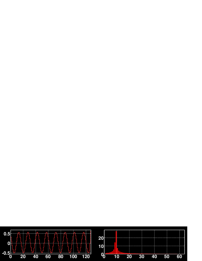
Figure 6.1: Example of a $10$ kHz oscillating signal. The left hand display shows the pressure signal in mPa and the right hand plot shows the magnitude of the DFT. In the pressure signal the $x$-axis corresponds to sample number, there are $128$ samples in the event window producing $64$ harmonics in the DFT. A clear peak in the tenth harmonic of the DFT is indicative of a single frequency sinusoidal composition at $\sim 10$ kHz.

Discrimination of sinusoidal signals is aided by the fact that they show distinct, isolated peaks in the DFT. If a sinusoidally oscillating signal has a period that is an integer number of sampling periods, a peak occupying a single bin in the DFT would be observed. However, in the case plotted in Figure 6.1, the signal period is $100$ µs and the sampling period is $128/140000=914.29$ µs. This mismatch is the source of the tails either side of the peak in the tenth harmonic in the DFT; the effect is known as leakage.

6.3.2 Categorisation of events

Of the $12,453,500$ reduced events, $3526$ corresponded to multiplicities of four or greater above the $35$ mPa threshold with an equivalent frequency composition as identified in the DFT. The number of triggers per hydrophone and the trigger frequencies are plotted in Figure 6.2.

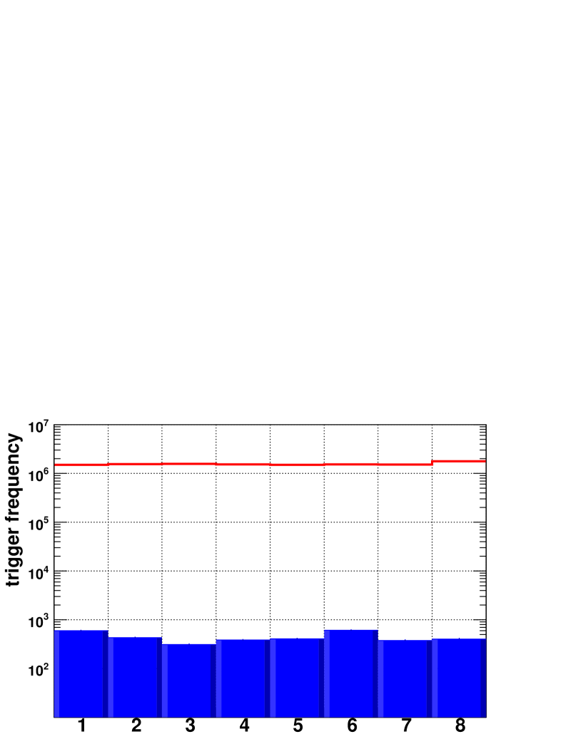
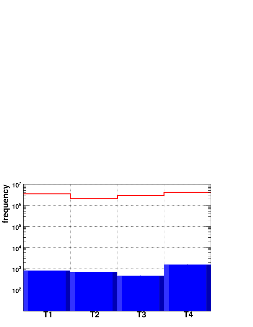
Figure 6.2: The number of triggers before (unfilled) and after (filled) cuts on each hydrophone at Rona, as retained by the data reduction code (Left). The number of instances if each trigger (Right).

Oscillating signals

One hundred and twenty-nine of the $3526$ events that passed the selection criteria were signals of a sinusoidally oscillating nature. These events, whilst originally being classified as calibration tones, did not occur at occasions when a Rona calibration tone was scheduled to be injected into the system, as recorded in the recorder logbook entries. Nor were the frequencies consistent with those injected by the Rona operators. An example of such a signal is plotted in Figure 6.3.

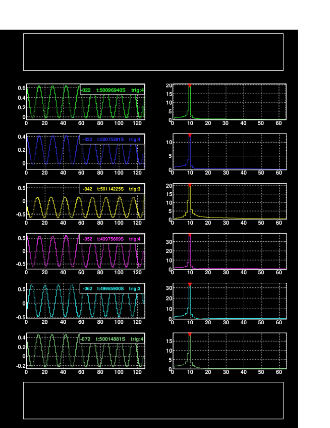
Figure 6.3: A $10$ kHz event coincident on six hydrophones showing a clear sine wave component. Traces are Pressure (Pa) (Left) and DFT magnitude (Right). Sample number runs along the $x$-axis.

The source of these signals is currently unknown but it is suggested that they represent an anthropogenic background as opposed to bio-acoustical or environmental noise. All of the $10$ kHz oscillating signals identified in this analysis occurred on 14/12/2005 between 11:24 and 14:14. Two higher frequency oscillating signals were recorded with a five-fold coincidence at 10:24 on 14/12/2005 at 10:24, one high frequency signal on 16/12 at 04:44 and one further high frequency oscillating signal on 24/12 at 07:33. An example of one of the high frequency hydrophone traces is plotted in Figure 6.4, the remainder of the oscillating signals being at $10$ kHz.

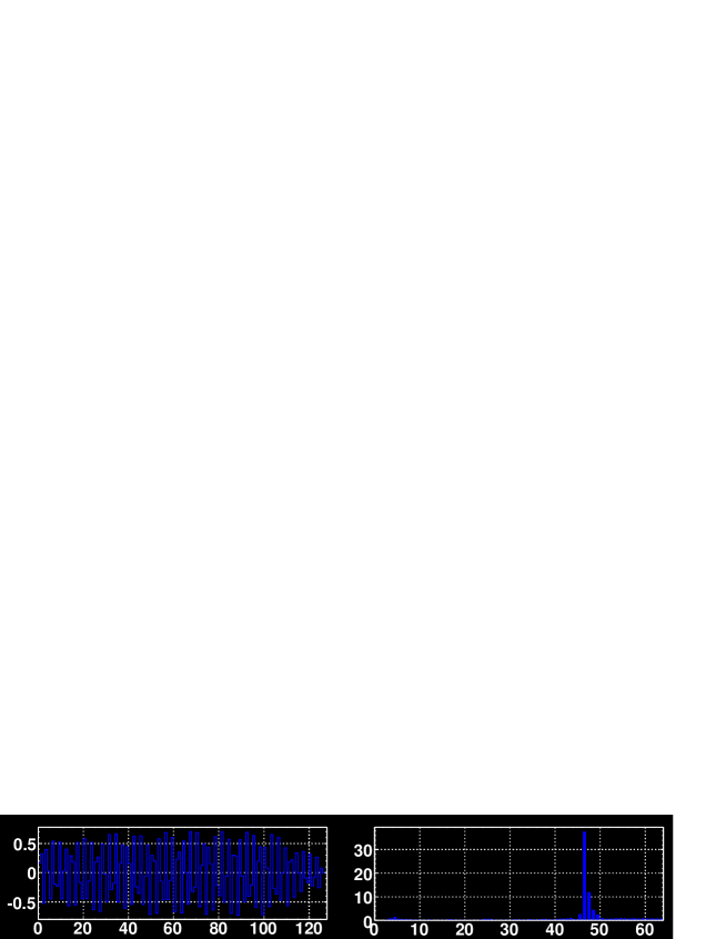
Figure 6.4: Example of a high frequency signal at Rona. The peak of the DFT is in the $46$th harmonic, corresponding to a frequency of $\sim 50$ kHz.

Transient events

The remaining $3397$ events were further subcategorised in terms of their frequency composition. Firstly the DFT of an event was analysed and classified as one of three types: smooth, mixed, or peaky as according to the criteria in Table 6.1.

Peakiness	Mean Number of Peaks in DFT
smooth	$\overline{N}_{\mathrm{peaks}}<2.5$
mixed	$\overline{N}_{\mathrm{peaks}}=2.5$
peaky	$\overline{N}_{\mathrm{peaks}}>2.5$

Table 6.1: Events were categorised in terms of their Peakiness, a variable determined by the number of peaks in the DFT.

The threshold for peakiness of $2.5$ is somewhat arbitrary but was chosen because it gave a good separation between events that showed a continuous DFT spectrum and those that showed a relative separation between peaks in the DFT. An example of two such events is plotted in Figures 6.6 and 6.6.

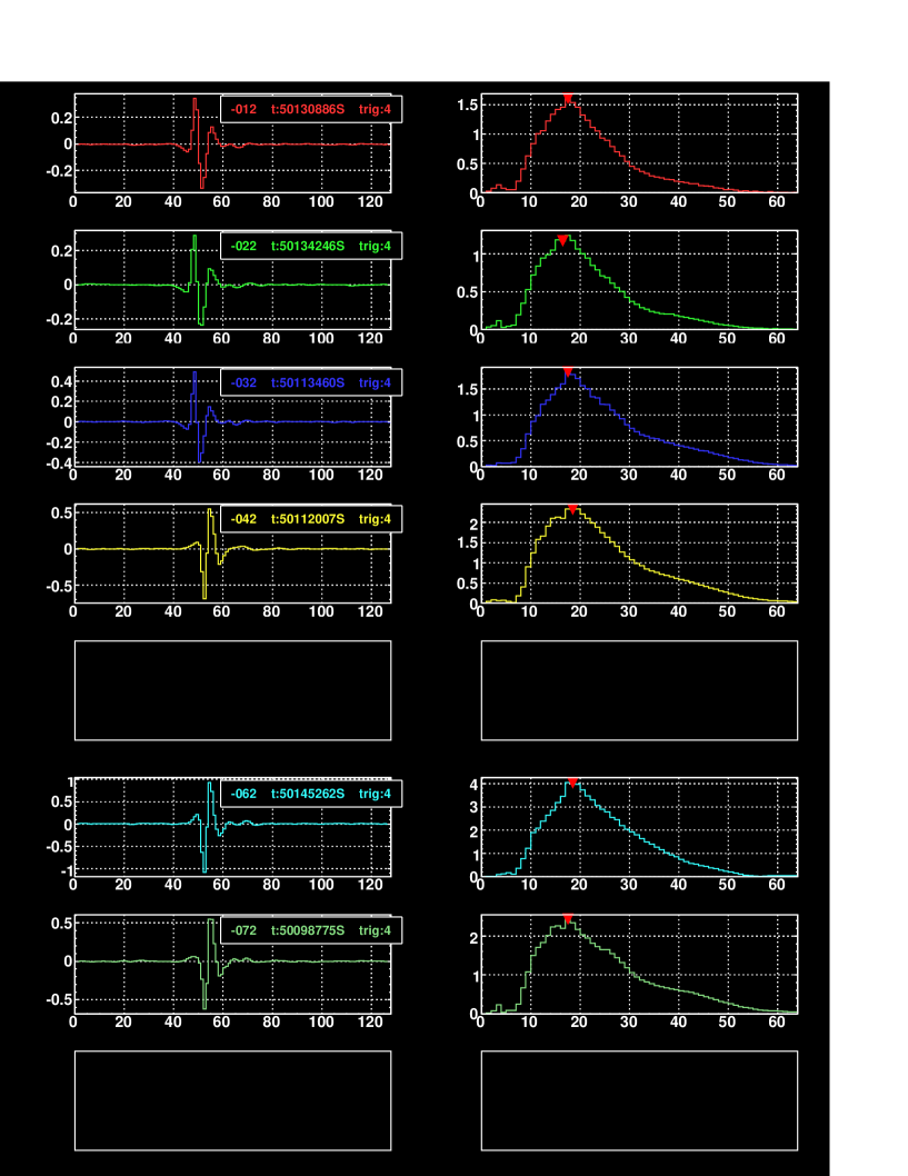
Figure 6.5: An event with a smooth DFT
$\overline{N}_{\mathrm{peaks}}=1$.

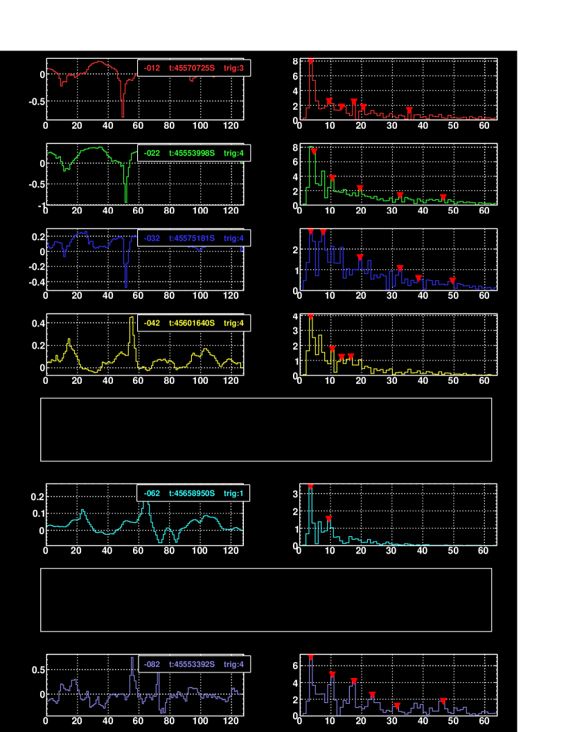
Figure 6.6: An event with a peaky DFT
$\overline{N}_{\mathrm{peaks}}=4.83$.

Observing the DFTs of the reduced Rona events, it is clear to see that there are two extremes in the acoustic data. The first is a periodic, oscillating signal such as the $10$ kHz sinusoid in Figure 6.3. This type of signal produces a distinct single peak in the DFT. The second is a type of signal evident in Figure 6.6. This appears to be an impulsive event, as indicated by the continuous DFT. The pulse shape of impulsive events is dominated by the impulse response of the hydrophone system whereas continuous oscillating signals show little contribution from the detector elements. Studying the shape of the DFT, i.e. their peakiness, thus gives an insight on the nature and origin of these events.

Analysis of the remaining $3397$ events that did not categorise as sinusoidally oscillating signals yielded $2329$ smooth, $44$ mixed and $969$ peaky signals. These events were further sub-categorised in terms of the magnitude of their frequency components according to the criteria in Table 6.2.

Frequency Range (kHz)		Mean DFT Harmonic
low	($\phantom{0}0<F<22$)	$0<\overline{\mathrm{DFT}}<20$
medium	($22<F<44$)	$20<\overline{\mathrm{DFT}}<40$
high	($44<F<70$)	$40<\overline{\mathrm{DFT}}<64$

Table 6.2: Rona events were sub-categorised according to the mean value of the DFT histogram.

No events satisfied the criteria for classification as high frequency. Only $55$ events classified as medium frequency events thus indicating a clear dominance of events below $\sim 22$ kHz.

6.3.3 Time dependence of events

Investigation into the temporal distribution of Rona events passing pressure and coincidence cuts suggests that activity is intermittent. There can be periods of sustained activity, lasting for several hours, showing events in every consecutive ten minute WAV file; and, there can be periods where a high number of events occur within a very short space of time, occupying only a single ten minute WAV file. The temporal variation in activity is best illustrated in a plot of event frequency as a function of time. Figure 6.7 shows this.

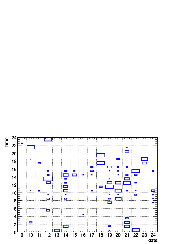
(a) 2D temporal distribution of Rona events

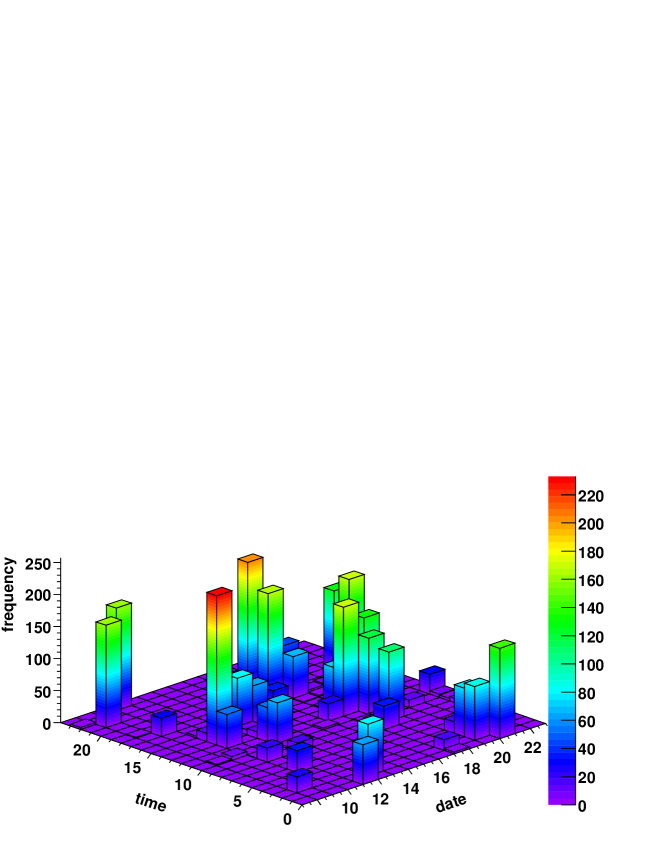
(b) $3D$ temporal distribution of Rona events

Figure 6.7: $2D$ and $3D$ plots of the temporal distribution of Rona events. Activity appears to be constrained to bursts of varying length and intensity. A large number of events can occur in a short space of time, producing isolated peaks such as the one at 21:00 on the 10th; or, events can be produced during a burst sustained over several hours such as the period between 08.00 and 16.00 on the 14th.

6.3.4 Recurring event types

Certain types of event, with distinct characteristics, are seen in the data on a recurring basis. An attempt has been made to categorise such events. Six distinct signal shapes have been identified. What follows is a brief description of each event type, ending with a table summarising the dates on which each of the events occur in the Rona data. For each type of event a single hydrophone signal inclusive of DFT is plotted, pressure in Pa runs along the $y$-axes and sample number along the $x$-axes. The full event displays showing coincidences can be found in Appendix E.

Short impulsive

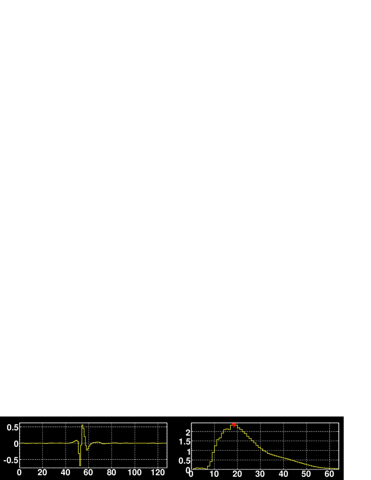
Figure 6.8: A short-lived impulsive event.

As already introduced in Section 6.3.2, there is a category of event that appears to display an impulsive component. It is categorised by a short duration multi-polar waveform and a continuous DFT. It is however indeterminable from the DFT alone whether the signal is actually the response of a hydrophone to an impulse or if it really is a bipolar signal with a $\sim 20$ kHz peak frequency as one might expect from an UHE hadronic cascade.

Low frequency oscillator

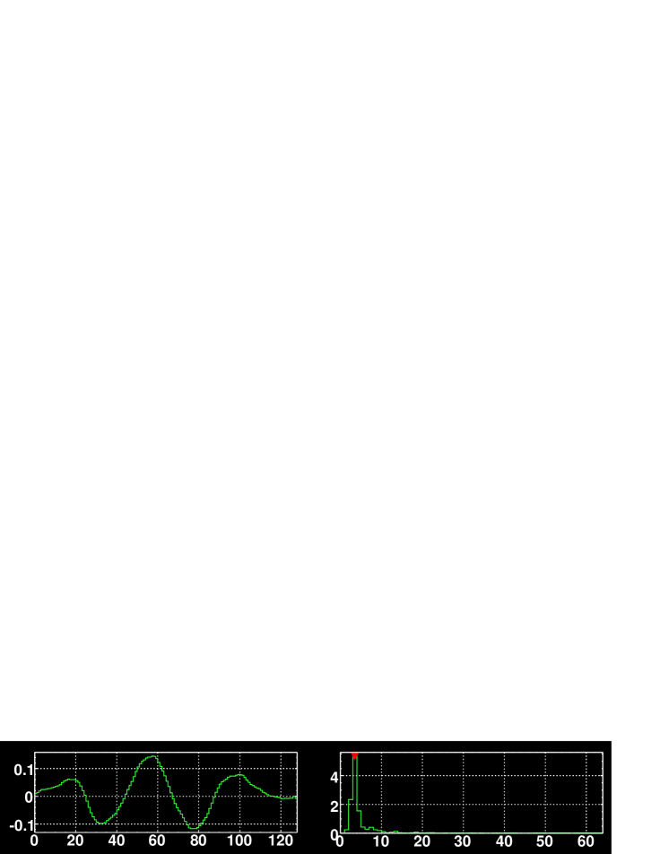
Figure 6.9: A low frequency oscillating event.

An event categorised by a low frequency ($\leq 4$ kHz) oscillating waveform appears consistently throughout the first fifteen days of Rona data. The pressure wave of these signals can often appear as in Figure E.2 or it can be somewhat distorted. Nevertheless this kind of signal is present in almost every day’s worth of data (see Table 6.3) and thus constitutes a significant background.

10kHz sinusoidal

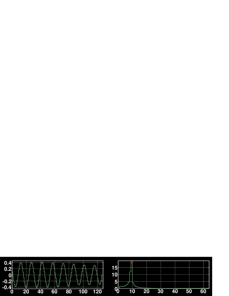
Figure 6.10: A $10$ kHz sinusoidally oscillating event.

Again, this signal has previously been introduced in Section 6.3.1. At first it was thought that these $10$ kHz oscillating signals were in fact calibration charges injected into the Rona DAQ to verify the integrity of transmission along the eight hydrophone to shore cables. However, this was later ruled out because they do not occur at times when the calibration tones were injected nor are they at the right frequency. Nonetheless, it is suggested that these signals are anthropogenic in origin.

High frequency oscillator

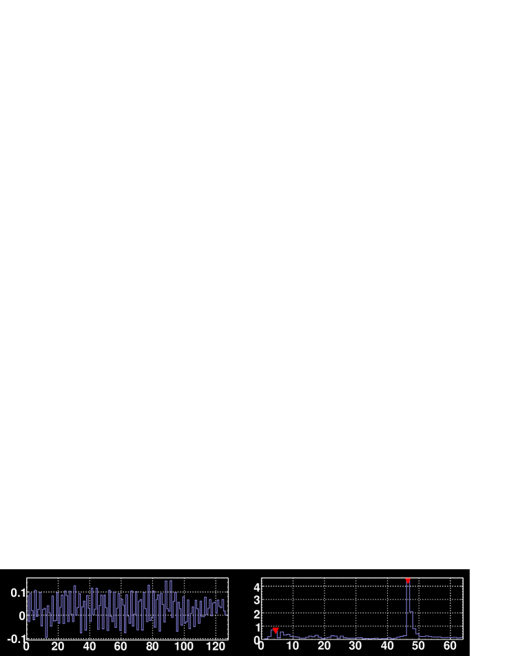
Figure 6.11: A high frequency event.

Higher frequency oscillating signals are also present in the Rona data but with a much lower abundance than the low frequency oscillators and the $10$ kHz sinusoids. Typically they occur at frequencies around $50$ kHz.

Ringer

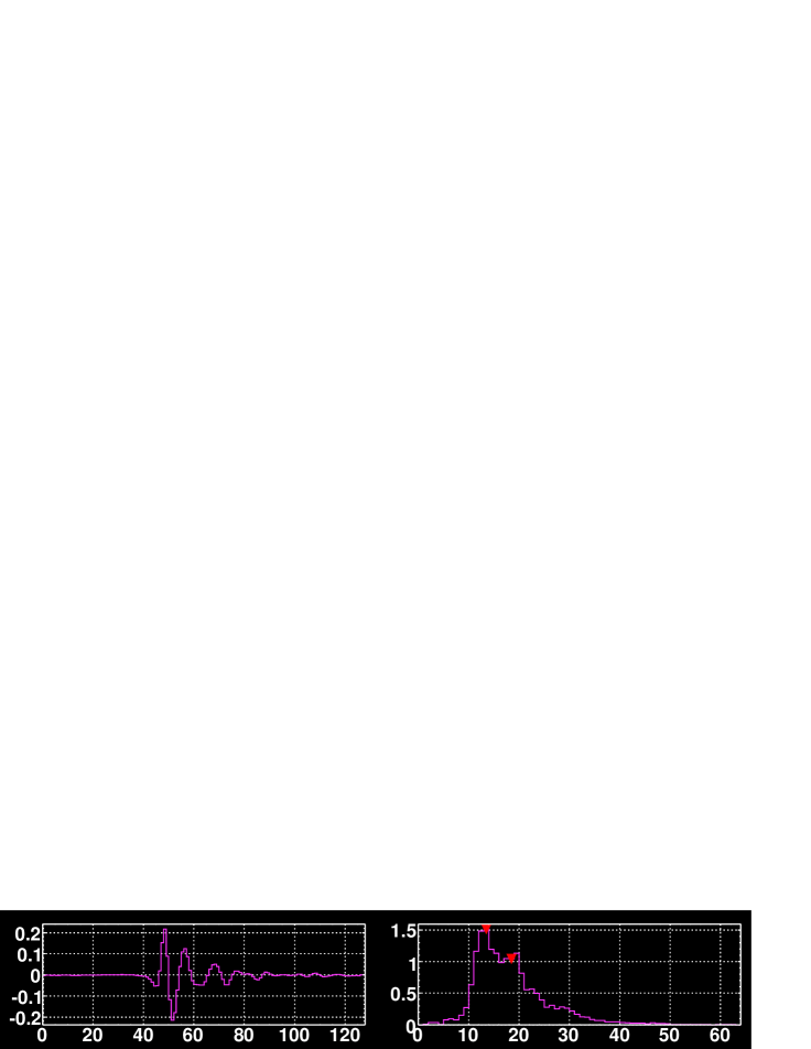
Figure 6.12: A ‘ringing’ event.

Some events in the Rona data occur periodically that demonstrate a decaying and oscillating pressure signal. There are two possible reasons for the appearance of such a signal: firstly, there is a decaying oscillating pressure wave in the water; secondly, due to a non-linearity in the phase response of the hydrophone system an asymmetric time delay of different Fourier components has caused the signal to ring. It is impossible to know for certain which of the two explanations is correct for any given case so these events have been arbitrarily labelled as “ringers”.

Bipolar

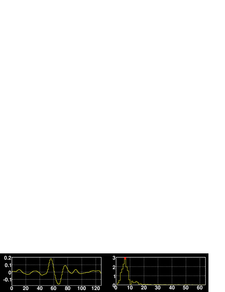
Figure 6.13: A ‘bipolar’ event.

Finally, this analysis has identified a class of event that is approximately bipolar in shape with a frequency close to that which we would expect from a neutrino induced particle cascade at some far-field distance from the Rona array. The signal is certainly not flat either side of the bipolar part of the pulse, and may indeed contain an oscillating component but one can imagine that if a smaller window had been chosen a clearer bipolar signal would be observed.

Clearly there are noise sources around the Rona array that can portray themselves as originating from UHE hadronic cascades. Further, more detailed work, beyond the scope of this somewhat qualitative analysis, is required to fully understand such backgrounds.

Occurrences of identified signal types

The identified signal types as described above recurred on several days throughout the data analysis. Table 6.3 summarises this information.

Event Type	Recurrence
Short impulsive	11th, 12th, 14th, 20th
Low frequency oscillator	9th-12th, 14th-17th, 19th-21st, 23rd
$10$ kHz sinusoidal	14th
High frequency	14th, 16th, 24th
Ringer	12th, 21st, 24th
Bipolar	17th, 19th-22nd, 24th

Table 6.3: Recurrence of events at Rona.

6.4 Summary

The DAQ as was in operation between 09/12 and 24/12/2005 at the Rona hydrophone array in Scotland has been described. Additionally a novel analysis of the raw $12,453,500$ events triggered by the ACoRNE data reduction has been reported. $3526$ passed offline cuts demanding that: there is a coincidence between four or more hydrophones; the peak pressure is above $35$ mPa; and, the maximum peak in the DFT of each coincident signal is at the same frequency. The requirement for four-fold or greater coincidence above a threshold of $35$ mPa puts the analysis in concordance with the sensitivity simulation described in previous chapters. Table 6.4 summarises the scale of coincidence amongst the analysed data. A total of $1059$ events showed a five-fold coincidence or greater. In Section 4.4 it was stated that for a mean noise level of $35.9$ dB only one false trigger in ten years, due to noise, with a five-fold coincidence should be observed. By integrating the energy of the pulses triggering the ACoRNE DAQ in this $15$ days worth of data, a noise level of between $90\to 100$ dB is observed, which demonstrates a higher level of noise activity than the location considered in the ACoRNE proposal. Furthermore it is suggested that there is an anthropogenic component of the Rona events that raises the noise level above that predicted by sea state alone. The noise at Rona provides an abundance of “signals”, the observation of which enables development of the data acquisition system. The more developed DAQ can then, in theory, be implemented elsewhere at a warmer, deeper and ultimately quieter site more suited to the acoustic detection of UHE neutrinos.

Level	4-fold	5-fold	6-fold	7-fold	8-fold
Frequency	2468	845	182	32	0

Table 6.4: Coincidences at Rona.

Chapter 7 Discussion and Outlook

7.1 The Motivation for Neutrino Astronomy

The motivation for Neutrino Astronomy is broad and compelling. As was discussed in the introduction the eventual first detection of neutrinos lagged their initial postulation by some twenty-three years. They are an essential component of the Standard Model of physics and are the second-most abundant known particle in the Universe yet their properties are still shrouded in mystery. One thing is for sure: the UHE $pp$ and $p\gamma$ interactions that follow the production of the highest energy cosmic rays will carry with them an associated flux of UHE neutrinos (Section 1.3.1). Due to their infinitesimal mass and lack of electric charge they can offer a unique perspective of the Cosmos. What is more, the scope for so-called “new physics” offered by Neutrino Astronomy is abundant, whether it is from the decay of exotics such as topological defects or relic big bang particles, or the annihilation of dark matter, neutrinos can offer a window into the frontier territories of quantum scale gravity, extra dimensions, super-symmetry and dark matter (Section 1.3.2).

7.2 The Current Scale of Development

The Neutrino Astronomy effort is a global endeavour extending across the surface of the Earth from pole-to-pole and above-and-below from high in the atmosphere to the depths of the sea (Sections 2.3, 2.4 and 2.5). It is because of the pioneering efforts of those such as the ill-fated DUMAND project and the long established lake Baikal experiment that today’s neutrino telescopes can look to the future and envisage a technology on the cubic kilometre scale and beyond. Despite such grand aspirations the field as a whole remains in its infancy when compared, say, to the status of radio astronomy and to a lesser extent UHECR and TeV gamma astronomy. One hopes that in the years to come the fruits borne by this labour can match that which is emerging from experiments such as AUGER and HESS in the present day.

The acoustic detection of UHE neutrinos is undoubtedly the least well developed technique. However it is arguably the most elegant in its simplicity. The direct detection of the thermoacoustic emission resulting from the interaction of UHE neutrinos at the Earth, with an off the shelf technology such as commercially available wide band hydrophones, is unrivalled in its potential to offer huge effective volumes without the necessity of complicated detector design.

7.3 Simulation of Acoustic Arrays

7.3.1 Neutrino interactions

The ACoRNE simulation work has continued to be developed following the formation of the collaboration. From calculations of the initial interaction of a neutrino at the Earth to the reconstruction of the thermoacoustic emission by cubic kilometre arrays of hydrophones a vast number of processes require consideration. Understanding the neutrino-nucleon cross-section at EeV energies depends on some combination of parameterised empirical data, extrapolated to higher energies, and theoretically motivated approximations. Man-made particle accelerators will likely never rival those of nature in their ability to accelerate particles to the highest energies. Presently it is from CR air shower experiments that we gain the most insight into particle interaction cross-sections at the TeV scale and beyond. Eventually neutrino telescopes, it is hoped, will provide the same quality of information as experiments such as HI-RES, KASCADE, AUGER and those alike, allowing the existing models that are relied upon in programs such as ANIS, PYTHIA and CORSIKA to be tuned to a finer degree of accuracy. For now we accept that the level of uncertainty in our particle interaction simulations is at worst within the level of individual event fluctuations (Sections 3.3.2 and Appendix B).

7.3.2 Formation and propagation of the signal

The formation of the bipolar acoustic signal characteristic of an UHE neutrino induced particle cascade relies exclusively on knowledge of the thermoacoustic energy deposited by the hadronic cascade. Efforts both experimental and theoretical have been made to best understand this mechanism. In the simulation work contained in this thesis, parameterisations of the integrated thermal energy resulting from the Geant4 and CORSIKA programs at various energies have been utilised to these ends (Section 3.4). Furthermore, the far-field approximation has been invoked to parameterise the peak pulse pressure, which has been shown to vary in direct proportion to the energy of the cascade.

The propagation of acoustic signals in the sea is as rich and diverse a field as Neutrino Astronomy. To attempt to incorporate something with such a magnitude of complexity into simple parameterisations of absorption, attenuation and propagation (Sections 4.2 and 4.3) is perhaps something of an injustice. Nevertheless progress will continue to be made upon the first generation codes that incorporated a constant velocity of sound towards more complicated ray-traced methods as described in this work, complex absorption models and beyond. Knowledge of the sound velocity profile surrounding a detector is critical to our understanding of its performance. Indeed we are fortunate that the deep sea presents something of an idealised situation in that the SVP is essentially linear, yet it remains to be seen exactly how accurate our understanding of it need be. What is more the boundary conditions at the sea surface and sea bed that have been neglected in this work present in themselves a broad subject for study. If the bipolar acoustic signal can undergo surface or sea bed reflections without experiencing too much distortion then the effective volume for a given array may extend well beyond the cutoff of $48$ km observed in this work.

7.3.3 Noise and filtering

The effects of noise and filtering again encompass a vast amount of research that is parameterised into the simple models utilised in the large scale detector simulation described in this thesis (Section 4.4). What is being learnt from experimental projects such as SAUND in the Bahamas, the acoustic branches of the ANTARES and NEMO collaborations at their respective sites, and from the ACoRNE project at Rona (Chapter 6) is that the backgrounds presented to the acoustic neutrino astronomer are numerous and multifaceted, presenting in themselves events that emulate the type of signal one may expect from an UHE neutrino induced particle cascade. Understanding of thresholds continues to develop as data are gathered from arrays such as those operated by the aforementioned groups and so does the continuing development of matched filters.

7.3.4 The large scale detector simulation

The reconstruction algorithms developed as part of this work represent the first iteration in what will undoubtedly mature into a vastly more complex field of study. Sensitivity predictions for acoustic arrays at present represent the work of a handful of people working broadly in isolation. In addition to the development of the computerised models, described above, that effectively sit as a front-end to the large scale simulation there is scope for further refinement of the techniques, already in use in this study, with respect to vertexing, pointing and calorimetry (Sections 5.4, 5.6 and 5.8). Better development of the minimisation procedure has already been alluded to (Section 5.4.2), additionally optimising the reconstruction of the acoustic pancake remains an interesting and open matter for study. One can envisage much improved performance by fully exploiting the unique pancake geometry.

The nature of this work, as it was conceived in the beginning, was to consider typically one thousand hydrophones in a volume of one cubic kilometre. We have seen that there are different factors for which array density can be optimised such as the effective volume and the reconstruction performance (Sections 5.5 and 5.6). Naturally if one were to begin a proposal to design and build a dedicated acoustic array for the purpose of UHE neutrino astronomy extra considerations such as cost and deployability come into play; the randomly distributed arrays investigated here may practically be very difficult to manufacture. Clearly there is a great deal of research potential for proper optimisation of the geometry of an acoustic array.

With respect to the sensitivity predictions made here (Section 5.9), there is broad agreement with the work published in reference [69], (which recursively agrees with predictions from the IceCube collaboration). In loose terms, as current predictions stand, one requires a pressure threshold around $5-10$ mPa operating across an array of over a thousand cubic kilometres with at least one hundred hydrophones per cubic kilometre if the proposed flux of GZK neutrinos is to be observed. Given further study and development of array optimisation and reconstruction algorithms, this may change.

7.4 Predictions for Future Work

Within the field of acoustic neutrino astronomy there is now some idea of the scales (thousands of cubic kilometres) to be considered if one wants to guarantee observation of those neutrinos resulting from the attenuation of UHECRs by the cosmic microwave background radiation. Undoubtedly that level of commitment is years beyond today’s level of activity. Currently, acoustic projects exist by utilising existing infrastructures, be it through military hardware such as the AUTEC and Rona arrays used by SAUND and ACoRNE respectively, or by piggybacking the deployment of existing sea or ice based detectors such as ANTARES, NEMO and IceCube. This latter strategy paves the way for hybrid detection. Because water doesn’t facilitate radio detection and there is no overlap in energy for simultaneous optical and acoustic detection of a given neutrino (see Figure 2.15), ice is surely the best medium for hybrid detection. This is further enhanced by its higher density and longer light absorption lengths than for water, coupled with the potential for shear wave acoustics thanks to the lattice-like structure of ice. Within the IceCube collaboration work is underway to extend to hybrid optical/radio/acoustic detection. Any detector offering simultaneous registration of the same event via two independent means has intrinsically less systematic uncertainty. One as yet unanswered question that remains for the acoustic neutrino astronomer is that of positively identifying a signal as being that of a neutrino and completely ruling out any other source. Naturally a coincident radio based detection would remove a great deal of uncertainty.

As the ANTARES project nears full deployment the boreal cubic kilometre scale neutrino telescopes begin their design phases. Acoustic instrumentation is already a part of the ANTARES design scheme and is almost certainly going to feature in the next generation telescopes in the Mediterranean. If this existing infrastructure can be utilised in such a way as to provide readout for acoustic detection then the first cubic kilometre, sea-based acoustic neutrino telescopes may not be far away thus completing complementary neutrino telescopy in both the northern and southern hemispheres, a requisite for full sky coverage. The neutrino-light in which the Earth bathes will soon illuminate the world’s largest active particle detectors and enlighten physicists to the mysteries foretold by nature’s most enigmatic cosmic messenger.

Appendix A Empirical Data

A.1 Neutrino-Nucleon Cross Section

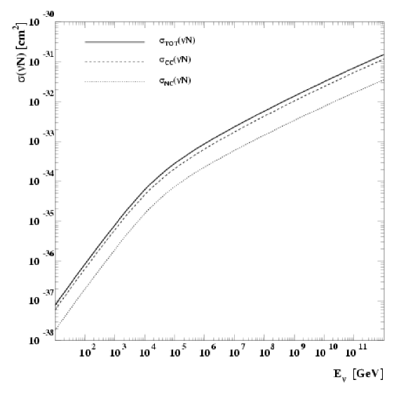
Figure A.1: The total neutrino-nucleon cross section and its charged current and neutral current contributions. Taken from [88]. The cross section for neutrino interactions at UHE was extrapolated from this plot and translated into the following code:

  // log10(sigma/cm^2) = -32.60 + (0.362*(log10(E/GeV)-7))
  // INPUT  : energy in eV
  // OUTPUT : cross section in cm^2

  double egev    = energy/1E09;
  double log10cs = -32.60 + (0.362*(log10(egev)-7.0));
  return pow(10,log10cs);

A.2 Knudsen Noise Curves

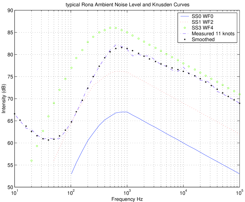
Figure A.2: Typical Knudsen noise curves (SS0, SS1, SS3) at the RONA site off the west Scottish coast used by the ACoRNE collaboration. These curves parameterise the ambient noise levels as a function of Sea States as defined by the World Meteorological Organisation. Also included is the measured noise level at Rona (Refer to legend).

Appendix B Comparison of Hadronic Showers from Geant4 and CORSIKA

The longitudinal and radial profiles of thermal energy deposition from hadronic cascades produced by two programs: Geant4 and CORSIKA are compared. The CORSIKA program, designed for the production of UHECR induced air showers, in the upper atmosphere of Earth, has been modified to produce hadronic cascades resulting from UHE neutrinos in a seawater medium [72].

In each case the average of $100$ showers is plotted to smooth out fluctuations on an event by event basis. The agreement between the shower shapes from Geant4 and CORSIKA is within the $20\%\to 30\%$ fluctuations seen between showers and the $\sim 30\%$ uncertaintity between choice of theoretical models in each program.

The modified version of CORSIKA has been developed so thermal energy densities for hadronic cascades initiated by primaries beyond the $100$ TeV limit inherent to Geant4 can be produced. Hence the extrapolated pressure to energy parameterisation need not be relied upon. A study of shower shapes and peak pulse pressure resulting from CORSIKA showers has however validated the assumption that pressure scales linearly with shower energy.

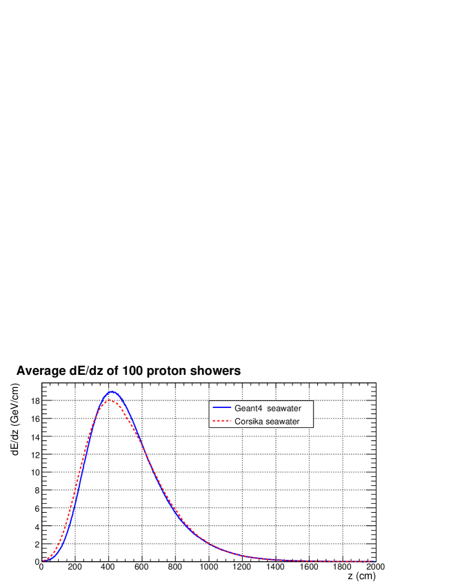
Figure B.1: Geant4 and CORSIKA longitudinal energy deposition at $10^{4}$ eV.

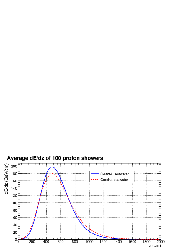
Figure B.2: Geant4 and CORSIKA longitudinal energy deposition at $10^{5}$ eV.

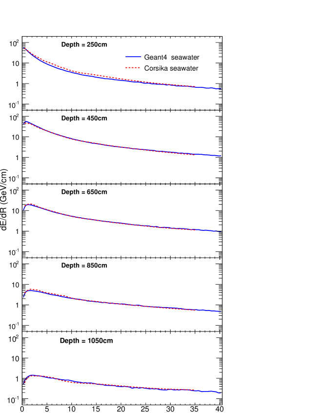
Figure B.3: Geant4 and CORSIKA radial energy deposition at $10^{4}$ eV for various depths along the shower axis.

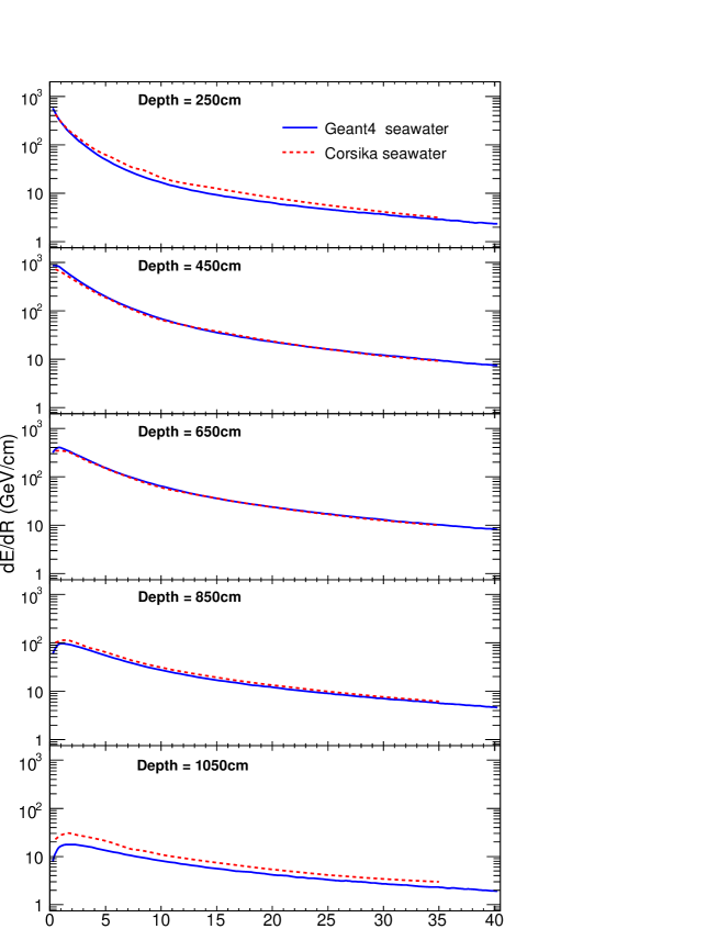
Figure B.4: Geant4 and CORSIKA radial energy deposition at $10^{5}$ eV for various depths along the shower axis.

Appendix C Formalism of Ray Tracing Algorithm

We start with the differential equations for ray paths in inhomogeneous (meaning the velocity of sound is not constant) media as given in [82] and proceed through the derivation therein:

$$\frac{d}{ds}\Big{(}n\frac{dx}{ds}\Big{)} = \frac{\partial n}{\partial x}$$ (C.1)

$$\frac{d}{ds}\Big{(}n\frac{dy}{ds}\Big{)} = \frac{\partial n}{\partial y}$$ (C.2)

$$\frac{d}{ds}\Big{(}n\frac{dz}{ds}\Big{)} = \frac{\partial n}{\partial z}$$ (C.3)

where index of refraction $n=c_{n}/c$ and $c_{n}$ is the velocity when the angle $\theta$ of the ray with respect to the horizontal is $0$. If the velocity $c$ is a function of $z$ only then $n=n(z)$ and Equations C.1 through C.3 are reduced to:

$$n\frac{dx}{ds} =$$ constant

$$n\frac{dy}{ds} =$$ constant

$$\frac{d}{ds}\Big{(}n\frac{dz}{ds}\Big{)} = \frac{dn}{dz}$$ (C.4)

We can arbitrarily collapse into $2$ dimensions by observing that the first two equations imply the ray path lies in a plane orthogonal to the $xy$-plane.

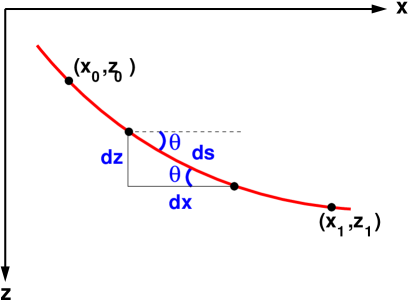
Figure C.1: Geometry of a single curved ray in a medium with varying sound velocity.

From Figure C.1 we see:

$$\frac{dx}{ds} = \cos\theta$$

$$\frac{dz}{ds} = \sin\theta$$ (C.5)

Taking the first equation of Equation C.4 and substituting the first equation from Equation C.5:

$$\frac{\cos\theta}{c}=\frac{1}{c_{n}}=K$$ (C.6)

which is Snell’s Law. $K$ is called the ray parameter which, for the geometry in Figure C.1 can be conveniently written as:

$$K=\frac{\cos\theta_{0}}{c_{0}}=\frac{\cos\theta_{1}}{c_{1}}$$ (C.7)

where $c_{0},\theta_{0}$ and $c_{1},\theta_{1}$ are the sound velocity and angle at $(x_{0},z_{0})$ and $(x_{1},z_{1})$ respectively. Substituting the second equation from Equation C.5 into the second equation in Equation C.4 we have:

$$\frac{dn}{dz} = \frac{d}{ds}(n\sin\theta)$$

$$= n\frac{d\sin\theta}{ds}+\sin\theta\frac{dn}{ds}$$

$$= n\cos\theta\frac{d\theta}{ds}+\sin\theta\frac{dn}{ds}$$

$$= n\cos\theta\frac{d\theta}{ds}+\sin\theta\frac{dn}{dz}\frac{dz}{ds}$$

$$= n\cos\theta\frac{d\theta}{ds}+\sin^{2}\theta\frac{dn}{dz}$$

which can be solved for $d\theta/ds$,

$$\frac{d\theta}{ds} = \frac{\cos\theta}{n}\frac{dn}{dz}$$ (C.8)

$$= -\frac{\cos\theta}{c}\frac{dc}{dz}$$

$$= -K\frac{dc}{dz}$$

This yields the important result that the curvature of the ray $d\theta/ds$ is directly proportional to the velocity gradient $dc/dz$. From the geometry in Figure C.1 we can see that

$$\frac{dx}{dz}=\cot\theta$$ (C.9)

such that horizontal range of the ray is given by:

$$dx = \cot\theta dz$$

$$x_{1}-x_{0} = \int_{z_{0}}^{z_{1}}\cot\theta dz$$ (C.10)

The travel time along the ray is given by:

$$dt = \frac{ds}{c}$$

$$t_{1}-t_{0} = \int_{z_{0}}^{z_{1}}\frac{ds}{c}$$

$$t_{1}-t_{0} = \int_{z_{0}}^{z_{1}}\frac{dz}{c\sin\theta}$$ (C.11)

Similarly, from the geometry in Figure C.1, the ray path length is given by:

$$ds = \frac{dz}{\sin\theta}$$

$$s_{1}-s_{0} = \int_{z_{0}}^{z_{1}}\frac{dz}{\sin\theta}$$ (C.12)

In the case of a linear sound velocity gradient:

$$c = c_{m}+gz$$

$$\frac{dc}{dz} = c^{\prime}=g$$ (C.13)

where the second term is the derivative with respect to $z$ of the first. We can now substitute the differential form of Equation C.13 into Equation C.8:

$$\frac{d\theta}{ds}=-Kg$$ (C.14)

$d\theta/ds$ is the curvature of the ray, and for a linear sound velocity gradient is constant. Hence the ray trajectory follows the arc of a circle. The radius of curvature $R$ is given by:

$$R_{c}=\frac{1}{|d\theta/ds|}=\frac{1}{|-Kg|}$$ (C.15)

Equations C.10, C.11 and C.12 for horizontal range, travel time and path length respectively can be expressed in terms of $\theta$. Starting with Equation C.10 we have:

$$x_{1}-x_{0} = \int_{z_{0}}^{z_{1}}\cot\theta dz$$

$$= \int_{z_{0}}^{z_{1}}\frac{\cos\theta}{\sin\theta}$$

$$= \int_{\theta_{0}}^{\theta_{1}}\frac{\cos\theta d\theta}{Kc^{\prime}}$$

where we have used $dz/\sin\theta=-d\theta/Kc^{\prime}$ obtained by differentiating Snell’s Law:

$$\cos\theta = Kc$$

$$\frac{d\cos\theta}{dz} = Kc^{\prime}$$

$$\frac{\sin\theta\,d\theta}{dz} = -Kc^{\prime}$$

$$\frac{dz}{\sin\theta} = -\frac{d\theta}{Kc^{\prime}}$$

The integral now becomes:

$$x_{1}-x_{0} = -\int_{\theta_{0}}^{\theta_{1}}\frac{\cos\theta\,d\theta}{Kg}$$

$$= -\frac{1}{Kg}[\sin\theta]_{\theta_{0}}^{\theta_{1}}$$

$$= \frac{1}{Kg}(\sin\theta_{0}-\sin\theta_{1})$$

$$= \frac{c_{0}}{g}\Big{(}\frac{\sin\theta_{0}-\sin\theta_{1}}{\cos\theta_{0}}\Big{)}$$

Similarly, starting with Equation C.11:

$$t_{1}-t_{0} = \int_{z_{0}}^{z_{1}}\frac{dz}{c\sin\theta}$$

$$= -\int_{\theta_{0}}^{\theta_{1}}\frac{d\theta}{g\cos\theta}$$

$$= -\frac{1}{g}\ln\Bigg{\{}\frac{\sec\theta_{1}+\tan\theta_{1}}{\sec\theta_{0}+\tan\theta_{0}}\Bigg{\}}$$

$$= -\frac{1}{g}\ln\Bigg{\{}\frac{\tan\Big{(}\frac{\theta_{1}+\pi/2}{2}\Big{)}}{\tan\Big{(}\frac{\theta_{0}+\pi/2}{2}\Big{)}}\Bigg{\}}$$

$$= -\frac{1}{g}\ln\Bigg{\{}\frac{\cos\theta_{0}(1+\sin\theta_{1})}{\cos\theta_{1}(1+\sin\theta_{0})}\Bigg{\}}$$

Finally from Equation C.12:

$$s_{1}-s_{0} = \int_{z_{0}}^{z_{1}}\frac{dz}{\sin\theta}$$

$$= -\int_{\theta_{0}}^{\theta_{1}}\frac{d\theta}{Kg}$$

$$= \frac{1}{Kg}{\theta_{0}-\theta_{1}}$$

$$= \frac{c_{0}}{g\cos\theta_{0}}(\theta_{0}-\theta_{1})$$

One can formulate an equation for the change in depth of the ray directly from Equation C.13 by using Snell’s Law as given in Equation C.7. From:

$$z=\frac{c-c_{m}}{g}$$

One can write:

$$z_{1}-z_{0} = \Bigg{(}\frac{c_{1}-c_{m}}{g}\Bigg{)}-\Bigg{(}\frac{c_{0}-c_{m}}{g}\Bigg{)}$$

$$= \frac{c_{1}-c_{0}}{g}$$

$$= \frac{1}{g}\Bigg{(}c_{0}\frac{\cos\theta_{1}}{\cos\theta_{0}}-c_{0}\Bigg{)}$$

$$= \frac{c_{0}}{g\cos\theta_{0}}(\cos\theta_{1}-\cos\theta_{0})$$

In summary, when the sound velocity gradient is constant, the horizontal range, travel time, ray path length and change in depth are given by:

$$x_{1}-x_{0} = \frac{c_{0}}{g}\Bigg{(}\frac{\sin\theta_{0}-\sin\theta_{1}}{\cos\theta_{0}}\Bigg{)}$$ (C.16)

$$t_{1}-t_{0} = -\frac{1}{g}\ln\Bigg{\{}\frac{\cos\theta_{0}(1+\sin\theta_{1})}{\cos\theta_{1}(1+\sin\theta_{0})}\Bigg{\}}$$ (C.17)

$$s_{1}-s_{0} = \frac{c_{0}}{g\cos\theta_{0}}(\theta_{0}-\theta_{1})$$ (C.18)

$$z_{1}-z_{0} = \frac{c_{0}}{g\cos\theta_{0}}(\cos\theta_{1}-\cos\theta_{0})$$ (C.19)

Equations C.17, C.18, C.19 and C.19 form the basis for the ray tracing algorithm.

Appendix D Neutrino Source Data

The neutrino spectrum $E_{\nu}$, source distribution $(\rho,\theta,\phi)_{\nu}$ and interaction coordinates $(r,z,\phi)_{\mathrm{int}}$ as generated in the large scale detector simulation (Chapter 5) is summarised by the following plots (with energy in GeV, angles in radians and distances in metres):

Appendix E Recurring Event Types at Rona

The coincident signals for each event introduced in Section 6.3.4 are as follows:

Figure E.1: A short-lived impulsive event.

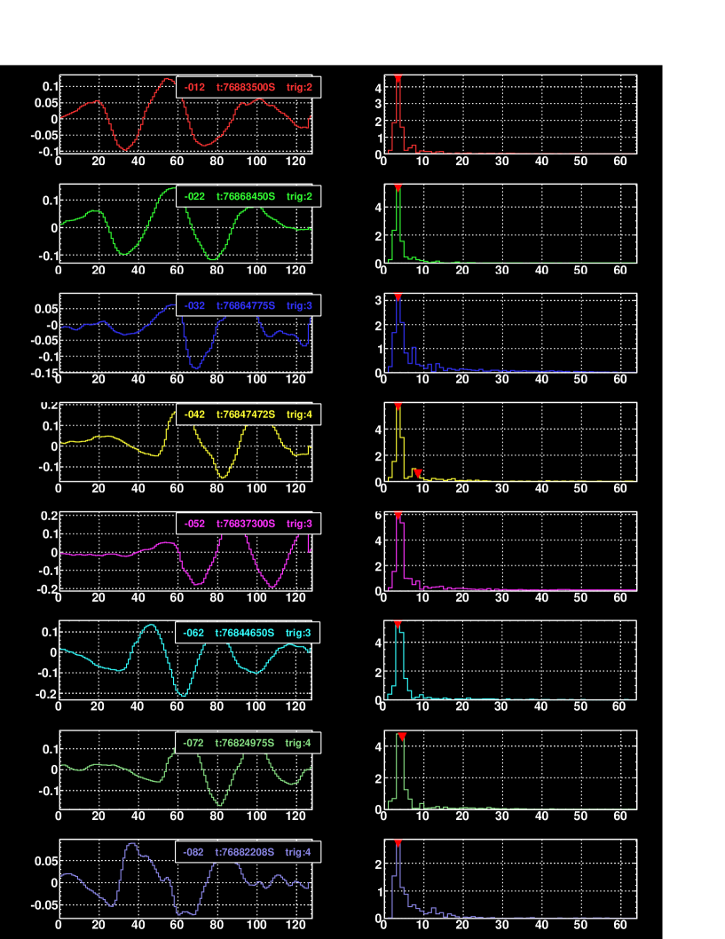
Figure E.2: A low frequency oscillating event.

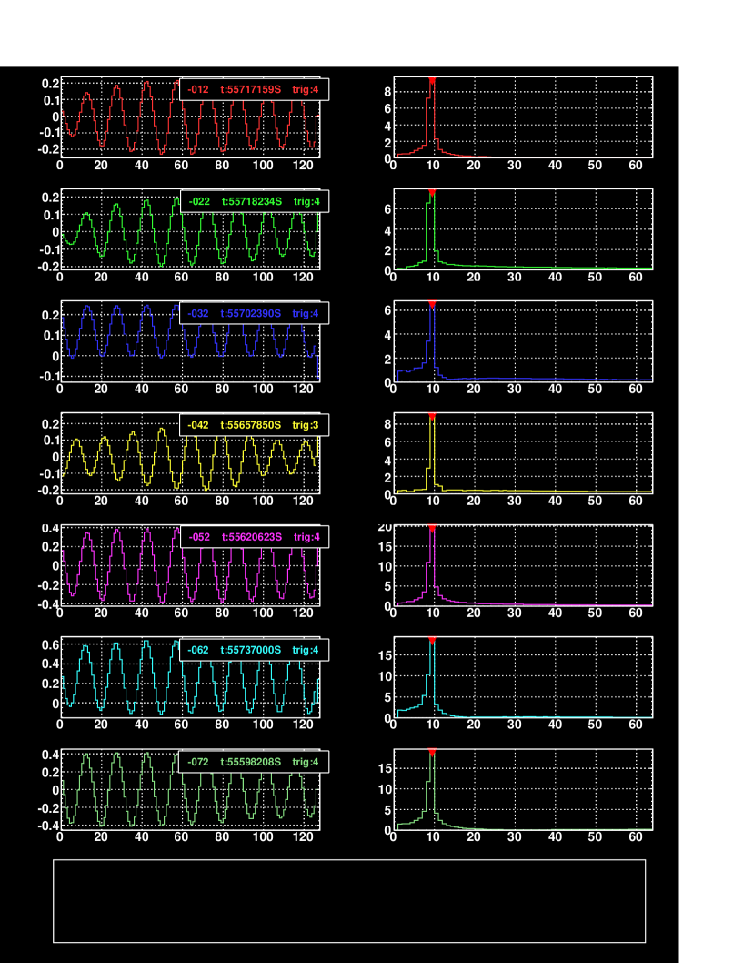
Figure E.3: A $10$ kHz sinusoidally oscillating event.

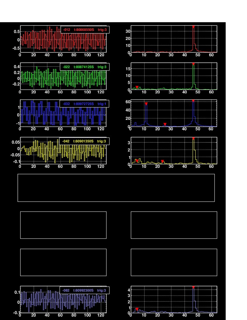
Figure E.4: A high frequency event.

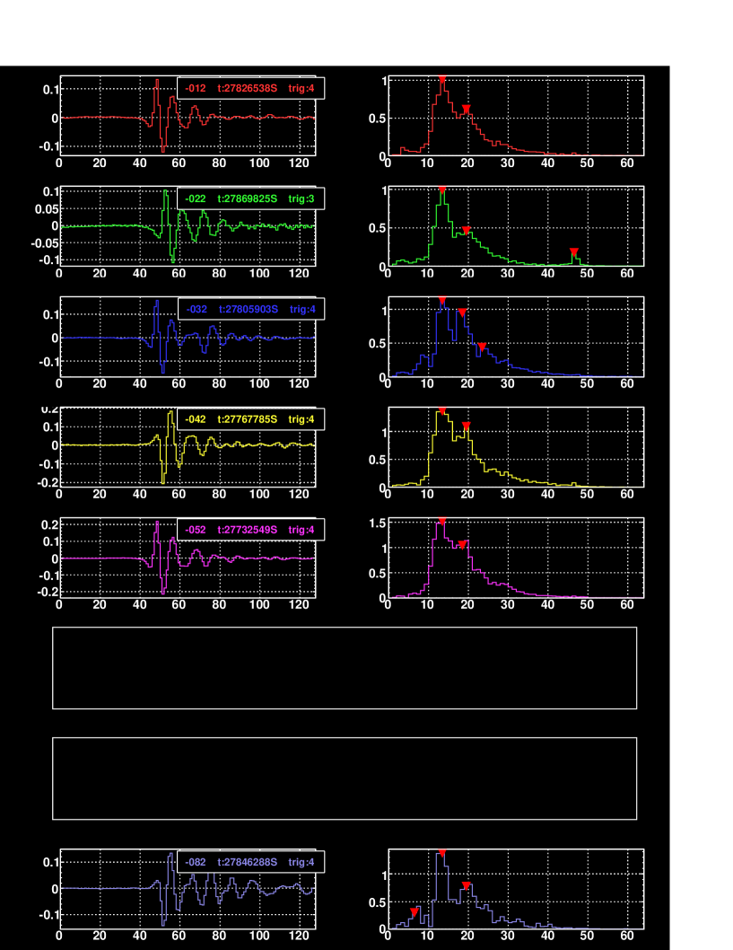
Figure E.5: A ‘ringing’ event.

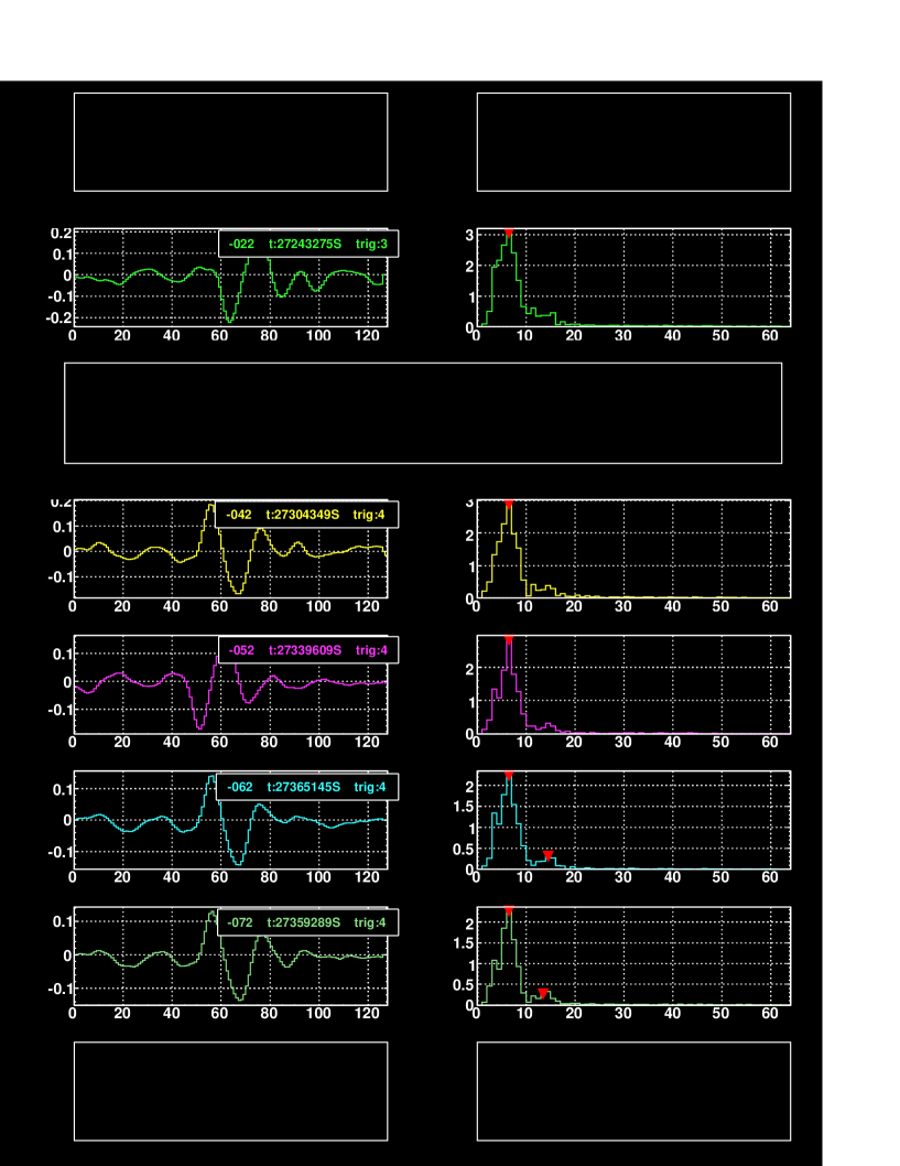
Figure E.6: A ‘bipolar’ event.

Bibliography

- [1] Modified by G. Gratta from an original by J. Learned and S. Pakvasa, http://kamland.stanford.edu/timeline/ accessed 16/02/2006, Website.
- [2] J. Chadwick, Verh. Deutsch. Phys. Ges. 16 (1914).
- [3] C. D. Ellis, Internat. Conf. on Phys. 15 (1934).
- [4] W. Pauli, Liebe Radioaktive Dammen und Herren, Open letter to the radioactive group during GAU excursion to Tübingen, 1930.
- [5] E. Fermi, Nuovo Cimento 11, 1 (1934).
- [6] F. Reines and C. L. Cowan, Jr., Phys. Rev. 92, 830 (1953).
- [7] Pontecorvo, B. and Gribov, V., Phys. Lett. 28B (1969).
- [8] R. Davis Jr., Phys. Rev. Lett 20, 1205 (1968).
- [9] M. L. Perl et al, Phys. Rev. Lett. 35, 1489 (1975).
- [10] K. Hirata, T. Kajita, M. Koshiba et al, Phys. Rev. Lett. 58 (1987).
- [11] R. M. Bionta, G. M. Blewitt, C. B. Bratton, et al, Phys. Rev. Lett. 58 (1987).
- [12] S. N. Ganguli, CERN-preprint (1989).
- [13] The Super-Kamiokande Collaboration, Phys. Rev. Lett. 81, 1562 (1998).
- [14] The DONUT collaboration: K. Kodama et al, Nucl. Inst. Meth. Phys. Res. A 493, 45 (2002).
- [15] The SNO Collaboration, Phys. Rev. Lett. 89 (2002).
- [16] The KAMLAND Collaboration, Phys. Rev. Lett. 90 (2003).
- [17] AMANDA Collaboration: J. Ahrens et al, Phys. Rev. Lett. 92 (2004).
- [18] F. Halzen, Submitted to EPJC (2006), astro-ph/0602132.
- [19] Y. Becherini, Talk given at TAUP 2005, Zaragoza, Spain (2006), astro-ph/0603570.
- [20] Ziro Maki, Masami Nakagawa, Shoichi Sakata, Prog. Theor. Phys. 28, 870 (1962).
- [21] Particle Data Group, The Particle Physics Booklet, 2002.
- [22] V. Berezinsky, Nuclear Physics B (Proc. Suppl.) 151, 260 (2006), astro-ph/0505220.
- [23] Diego F. Torres and Luis A. Anchordoqui, Rept.Prog.Phys. 67, 1663 (2004), astro-ph/0402371.
- [24] J. Cronin, T. K. Gaisser and S. P. Swordy, Sci, Amer. 276 (1994).
- [25] A. M. Hillas, Based on invited talk in ”Cosmology, Galaxy Formation and Astroparticle Physics on the pathway to the SKA”, Oxford, April, 2006, astro-ph/0607109.
- [26] John Bahcall, Eli Waxman, Phys.Rev. D 64 ((2001)), hep-ph/9902383.
- [27] E. Waxman, Invited review presented at the 33rd annual European Physical Society Conference, Rome, 2006, astro-ph/0607353.
- [28] J. S. Warren et al, Astrophys. J. 634, 376 (2005), astro-ph/0507478.
- [29] A. Dar, The origin of cosmic rays at all energies, in Proceedings of the 11th International Workshop on Neutrino Telescopes, pp. 451–476, 2005, astro-ph/0601329.
- [30] K. Greisen, Phys. Rev. Lett 16, 748 (1966).
- [31] G. T. Zatespin and V. A. Kuzmin, JETP. Lett 4, 78 (1966).
- [32] C. Aramo et al, Astropart.Phys. 23, 65 (2005), astro-ph/0407638.
- [33] P. Bhattacharjee and G. Sigl, Phys. Rep. 327, 109 (2000).
- [34] T. W. Kibble, J. Phys. A 9, 1387 (1976).
- [35] A. L. S. Khlebnikov, L. Kofman and I. Tkachev, Phys. Rev. Lett 81, 2012 (1998).
- [36] V. A. Kuzmin, Phys. Rep 320, 199 (1999), hep-ph/9903542.
- [37] Karl-Heinz Kampert (for the Pierre Auger Collaboration), Cosmic Rays at the Highest Energies – First Data from the Pierre Auger Observatory, 2006, astro-ph/0608136.
- [38] G. A. Askaryan, JETP 14, 441 (1962).
- [39] E. Andres et al, Astrophys. J 13, 1 (2000), astro-ph/9906203.
- [40] E. Andres et al, Nature 410, 441 (2001).
- [41] J. A. Aguilar, et al., submitted to Astropart. Phys (2006), astro-ph/0606229.
- [42] The DUMAND project http://www.phys.hawaii.edu/dumand/ accessed 02/05/2006.
- [43] V. Aynutdinov et al, Astropart. Phys. 25, 140 (2006), astro-ph/0508675.
- [44] G. Aggouras et al, Nucl. Inst. Meth. Phys. Res. A 552, 420 (2005).
- [45] P. Piattelli et al, Nucl. Phys. B. Proc. Suppl. 143, 359 (2005).
- [46] Igor Sokalski, The ANTARES experiment: past, present and future, in The Highest Energy Cosmic Rays and QCD, World Scientific, 2005, hep-ex/0501003.
- [47] Presented at VLVnT2 Workshop, Catania, Siciliy, Italy (2005), astro-ph/0606068.
- [48] D. Saltzberg and P. Gorham et al, Phys. Rev. Lett. 86 (2001).
- [49] S.W. Barwick et al, Phys. Rev. Lett. 96 (2006), astro-ph/0512265.
- [50] N. G. Lehtinen et al, Phys. Rev. D. 69 (2004), astro-ph/0309656.
- [51] P. Gorham et al, Phys. Rev. Lett. 93 (2004), astro-ph/0310232.
- [52] H.J.A. Rottgering et al, LOFAR - Opening up a new window on the Universe, in Cosmology, galaxy formation and astroparticle physics on the pathway to the SKA, 2006, astro-ph/0610596.
- [53] H. Falcke, Radio detection of cosmic rays with LOFAR and LOPES, presentation given at ”TeV Particle Astrophysics II”.
- [54] O. Scholten et al, Detecting UHE Cosmics & Neutrinos off the Moon; an Optimal Radio Window, in Acoustic and Radio EeV Neutrino Detection Activities, 2006, astro-ph/0609179.
- [55] I. Kravchenko et al, Astropart. Phys. 19, 15 (2003), astro-ph/0112372.
- [56] I. Kravchenko et al, submitted to Phys. Rev. D. 73 (2006), astro-ph/0601148.
- [57] P. Gorham et al, Nucl. Inst. Meth. A. 490, 476 (2002), hep-ex/0108027.
- [58] G. A. Askaryan, Sov. J. Atom Energy 3, 921 (1957).
- [59] J. G. Learned, Phys. Rev. D 19 (1979).
- [60] L. D. Landau and I. Ya. Pomeranchuk., Dokl. Akad. Nauk SSSR 92, 535 (1953).
- [61] A. Migdal, Phys. Rev. 103 (1956).
- [62] Nikolai G. Lehtinen et al, Astropart.Phys. , 279 (2002), astro-ph/0104033.
- [63] L. Sulak et al, Nucl. Inst. Meth. 161, 203 (1979).
- [64] K. Graf et al, Testing the thermo-acoustic sound generation in water with proton and laser beams, in Acoustic and Radio EeV Neutrino Detection Activities, pp. 127–131, World Scientific, 2006, astro-ph/0509450.
- [65] H. U. Sverdrup, Martin W. Johnson and Richard H. Fleming, The Oceans, Their Physics, Chemistry, and General Biology. (New York: Prentice-Hall, 1942).
- [66] The SAUND Collaboration, http://hep.stanford.edu/neutrino/saund accessed 14/03/2007, Website.
- [67] J. Vandenbroucke, G. Gratta and N. Lehtinen, Astrophys.J. 621, 301 (2005), astro-ph/0406105.
- [68] T. Montaruli for the ANTARES Collaboration, Neutrino Astronomy with ANTARES, in Proc. of XXXIV Int. Symposium on Multiparticle Dynamics, hep-ex/0410079.
- [69] T. Karg, Detection of ultra high energy neutrinos with an underwater very large volume array of acoustic sensors: A simulation study, PhD thesis, Universität Erlangen-Nürnberg, 2006.
- [70] A. Gazizov and M. P. Kowalski, Comput. Phys. Commun. 172, 203 (2005), astro-ph/0406439.
- [71] L. Lönnblad, Computer Phys. Comm 84, 307 (1994).
- [72] T. Sloan, Simulation of Ultra High Energy Neutrino Interactions in Ice and Water, Article submitted to Astropart. Phys., 2007.
- [73] S. Agostinelli et al, Nucl. Inst. Meth. Phys. Res. A 506, 250 (2003).
- [74] R. Brun and F. Rademakers, Nucl. Inst. Meth. in Phys. Res. A 389, 81 (1997).
- [75] H. Pi., Computer Phys. Comm. 71 (1992).
- [76] P.V. Degtyarenko, M.V. Kossov and H.P. Wellisch, Eur. Phys. J. A8, 217 (2000).
- [77] P.V. Degtyarenko, M.V. Kossov and H.P. Wellisch, Eur. Phys. J. A9, 411 (2000).
- [78] A. B. Kaidalov and K. A. Ter-Martirosyan, Physics Letters B 117, 247 (1982).
- [79] B. Andersson et al, Physics Reports 97, 31 (1983).
-
[80]
The ACoRNE Collaboration
accessible at http://pppa.group.shef.ac.uk/acorne.php PPARC PP/C504019 Accessed 07/02/2007, 2000. - [81] S. Danaher, Private communication.
- [82] C. A. Boyles, Acoustic waveguides: applications to oceanic science (New York: Wiley, 1984).
- [83] S. Danher, First Data from ACoRNE and Signal Processing Techniques, in Acoustic and Radio EeV Neutrino detection Activities, edited by L. Thompson and S. Danher, Institute Of Physics, 2006, in press.
- [84] F. James, MINUIT: Function Minimization and Error Analysis, Website.
- [85] Particle Data Group, J. Phys. G 33, 297 (2006).
- [86] R. Nahnhauer and S. Böser, editor, Acoustic and Radio EeV Neutrino detection Activities, World Scientific, 2005.
- [87] L. Thompson and S. Danaher, editor, Acoustic and Radio EeV Neutrino detection Activities, Institute Of Physics, 2006, in press.
- [88] J. Kwiecinski, A. D. Martin, A. M. Stasto, Acta Phys.Polon. B31, 1273 (2000), hep-ph/0004109.