Magnetization reversal driven by spin-injection : a mesoscopic spin-transfer effect

Abstract

A mesoscopic description of spin-transfer effect is proposed, based on the spin-injection mechanism occurring at the junction with a ferromagnet. The effect of spin-injection is to modify locally, in the ferromagnetic configuration space, the density of magnetic moments. The corresponding gradient leads to a current-dependent diffusion process of the magnetization. In order to describe this effect, the dynamics of the magnetization of a ferromagnetic single domain is reconsidered in the framework of the thermokinetic theory of mesoscopic systems. Assuming an Onsager cross-coefficient that couples the currents, it is shown that spin-dependent electric transport leads to a correction of the Landau-Lifshitz-Gilbert equation of the ferromagnetic order parameter with supplementary diffusion terms. The consequence of spin-injection in terms of activation process of the ferromagnet is deduced, and the expressions of the effective energy barrier and of the critical current are derived. Magnetic fluctuations are calculated: the correction to the fluctuations is similar to that predicted for the activation. These predictions are consistent with the measurements of spin-transfer obtained in the activation regime and for ferromagnetic resonance under spin-injection.

In the context of spintronics, spin transfer is a generic term that describes the magnetization reversal or magnetization excitations of a ferromagnetic layer provoked by the injection of a spin-polarized electric current. This effect has now been observed while measuring the magnetization of many different systems liste0 . It has also been implemented into the last generation of magnetic random access memories MRAM .

Spintronics immerged first with the discovery of spin-injection and giant magnetoresistance (GMR) GMR . Effects of spin-injection at a junction of a ferromagnet are successfully described within the two spin-channel model Johnson ; Wyder ; ValetFert ; Levy ; Weg . In this description, GMR, or spin-accumulation, is due to the spins of the conduction electrons that are driven out-of equilibrium by an interface: the difference of the electro-chemical potentials $\Delta\mu$ between the two spin-channels leads to a redistribution of the spin populations through spin-flip mechanisms. Depending on the magnetic state of the ferromagnet at the junction, this redistribution of spin-dependent electronic populations modifies the resistance. For this reason, the GMR can be used as a probe (e.g. read heads for hard disk drive) in order to measure precisely the position of a nanoscopic ferromagnetic moment in the corresponding configuration space. Inversely, from the point of view of the ferromagnetic properties, it is natural to expect that the spin-flip mechanism at the interface modifies locally the density of the magnetic moments in this configuration space. This is a consequence of both the spin-orbit coupling (or s-d relaxation), and the redistribution of spins in the magnetic configuration space. The spin-injection would then be responsible for a gradient of the density in the magnetic configuration space, that contributes to the diffusion processes of the ferromagnetic moment.

The aim of this work is to investigate the consequences of this redistribution mechanism for the ferromagnetic moments. This task is performed in the framework of the nonequilibrium theory of mesoscopic systems Rubi1 ; RubiFDT . In this context, the coupling between the spin of conduction electrons and the ferromagnetic order parameter is due to the introduction of a relevant Onsager cross-coefficient that links the spin-polarized electric currents (i.e. transport of mass, spins, and electric charges in the normal space) to the ferromagnetic current (i.e. a massless transport of ferromagnetic moments in the corresponding space). Physically, this spin-transfer cross-coefficient accounts for the fact that the spins of the conduction electrons also contribute to the transport of the ferromagnetic order parameter in the space of magnetic moments, in analogy with the thermoelectric Peltier-Seebeck cross-coefficient that accounts for the fact that charge carriers contribute also to the transport of heat.

The motivation for a classical mesoscopic analysis was the need to account for the following highly specific properties observed in spin-transfer experiments that can hardly be accounted for in direct microscopic approaches Slon ; Berger ; Miltat ; Revue . First, in single domain ferromagnets, the reversible part of the hysteresis loop is not significantly modified under current injection, while the irreversible jump is drastically modified Revue . Second, the amplitude of spin-transfer is proportional to the giant magnetoresistance and to the amplitude of the current MSU2 ; Jiang ; Manchon . Third, the Néel-Brown activation law is still valid under current injection, with a correction of the barrier height that is quasi-symmetric under both the permutation of the magnetic configuration (parallel to anti-parallel and inversely) and the change of the direction of the current MSU2 ; Moi ; Fabian ; Buhrman . ”Quasi”-symmetric means here that a quantitative shift (a factor 2 to 4 in general) is systematically observed in the amplitude of spin transfer for both transitions in spin-valve structures. Fourth, this last quasi-symmetry is also observed in the context of ferromagnetic resonance under current injection close to the equilibrium states (i.e. with an weak spin-injection) DienyRes . In order to compare the results of the model with these observations, after calculating the diffusive correction of the Landau-Lifshitz-Gilbert equation (LLG) due to spin-injection in the first section, the correction to activation law is derived in a second section, and the correction to the fluctuations is derived in the third section.

.1 Spin-injection correction to the ferromagnetic Landau-Lifshitz-Gilbert Equation

In the framework of the two conducting channel approximation, the system is described by two electronic populations. A first conducting channel is carrying the conduction electrons of spin up $\uparrow$ with the electric conductivity $\sigma_{\uparrow}$ and the other channel is carrying the electron conduction of spin down $\downarrow$ with the electric conductivity $\sigma_{\downarrow}$. The quantification axis is defined by the direction of the magnetization of the ferromagnet. The Ohm’s law is valid for each channel: in a 1D ferromagnetic wire described with a single space coordinate $z$, the electric current $J^{e}_{\uparrow}$ (resp. $J^{e}_{\downarrow}$ ) is related to the local electric field $E_{\updownarrow}=-\frac{1}{e}\frac{\partial\mu^{e}_{\updownarrow}}{\partial z}$ Levy through the conductivity: $J^{e}_{\updownarrow}=\sigma_{\updownarrow}E_{\updownarrow}$, where $\mu^{e}_{\uparrow}$ (resp. $\mu^{e}_{\downarrow}$) is the electrochemical potential of the channel of spins $\uparrow$ (resp. $\downarrow$).

In the case of an interface between a normal metal and a ferromagnet (or between two ferromagnets), the spin-dependent relaxation between both electronic populations leads to a redistribution of spins within the two channels, that is driven by the difference between the two electro-chemical potentials $\Delta\mu^{e}(z)=\mu^{e}_{\uparrow}-\mu^{e}_{\downarrow}$ (the ”spin-neutral” electrochemical potential is defined, in turns, by $\mu^{e}_{0}=\mu^{e}_{\uparrow}+\mu^{e}_{\downarrow}$). The parameter $\Delta\mu^{e}$ accounts for the spin-injection, or spin accumulation, mechanism (see Fig. 1). The equilibrium state of the spin system is recovered in the bulk where, by definition, $\Delta\mu^{e}(\infty)=0$. This corresponds to a distance of some few times the spin-diffusion length (some tens of nanometers in usual Co or Ni layers). The description can be generalized to multichannel model that includes the spins of the conduction electron of the $s$ band and of the spins of the conduction electrons of the $d$ band, with the corresponding interband relaxation MTEPW ; Revue . For convenience, a two-channel approximation is used in the following, in which we define $J_{0}^{e}=J^{e}_{\uparrow}+J^{e}_{\downarrow}$ as the ”spin-neutral” electrical current, and $\delta J^{e}=J^{e}_{\uparrow}-J^{e}_{\downarrow}$ is the spin-polarized electrical current.

The system under consideration is composed not only by the microscopic spins up and down carried by the conduction electrons of different nature (band $s$ or $d$), but also by a ferromagnet of length $v$ ( $v$ is also the volume in the normal space for a section unity) described by a ferromagnetic order parameter $\vec{M}$. The last variable is defined in the space of the ferromagnetic moments ( Fig. 2) of constant modulus : $\vec{M}=M_{s}\vec{u}_{r}$, called $\gamma$ - space in the following Prigogine . This space can be defined on the unit sphere (see Fig. 2) with the two angles $\theta$ and $\varphi$, the radial unit vector $\vec{u}_{r}$, the azimuth unit vector $\vec{u}_{\theta}$ and the zenith unit vector $\vec{u}_{\varphi}$ . The magnetization is then described statistically in the configuration space by the density $\rho^{F}(\theta,\varphi)$ of ferromagnetic moments oriented at a given direction $\gamma=\{\theta,\varphi\}$, and also by the ferromagnetic potential energy $V^{F}(\theta,\varphi)$ that contains at least the contributions due to the external magnetic field $\vec{H}$ and the anisotropy energy. Typically, for a uniaxial anisotropy with anisotropy constant $K$, the ferromagnetic potential writes: $V^{F}(\theta,\varphi)=Ksin^{2}(\theta)-M_{s}Hcos(\theta-\phi)$ where $\phi$ gives the direction of the applied field. This potential energy has the form of a double well potential (Fig. 2).

In the absence of spin-injection, the magnetization is a conserved variable, so that the conservation law writes $\frac{\partial\rho_{0}^{F}}{\partial t}=-div(\vec{j}_{0}^{F})$, where $\vec{j}_{0}^{F}=j_{0}^{F\theta}\vec{u}_{\theta}+j_{0}^{F\varphi}\vec{u_{\varphi}}$ is the ferromagnetic current density and the operator $div$ is the divergence defined on the surface of a unit sphere. This is no longer the case under spin-injection at an interface: due to the redistribution of spins in the different channels (especially from $s$ band to $d$ band) spins are transferred from one sub-system to the other, and the ferromagnetic sub-system becomes an open system. In order to work in a larger system that is closed, i.e. that does not exchange magnetic moments with the environment, the total ferromagnetic density $\rho^{F}_{tot}$ and total ferromagnetic current $\vec{j}_{tot}^{F}$ are defined in what follows.

In the total system, that includes both the ferromagnetic layer and the spin-polarized current, the entropy production d$\mathcal{S}$/dt (per unit of solid angle and per unit of length) is given by

$$\frac{d\mathcal{S}}{dt}=-\frac{1}{T}\left(\vec{j}_{tot}^{F}.\vec{\nabla}\mu^{F}-\delta J^{e}\frac{\partial{\Delta{\mu}^{e}}}{e\partial{z}}-J_{0}^{e}\frac{\partial{\mu_{0}^{e}}}{e\partial{z}}\right)$$ (1)

where $T$ is the temperature assumed uniform, $\vec{\nabla}$ is the gradient defined on the surface of the unit sphere, $\mu^{F}$ is the total ferromagnetic chemical potential, and $e$ the charge of the electron. The last term in the right hand side is the Joule heating, the second term is the dissipation related to the giant magnetoresistance, and the first term is the ferromagnetic dissipation that defines the total ferromagnetic current $\vec{j}_{tot}^{F}$ in the internal space of magnetic moments DeGroot .

From the expression of the entropy production Eq. (1) and the second law of thermodynamics d$\mathcal{S}/dt\geq 0$, the flux involved in the system are related to the generalized forces through the matrix of the Onsager transport coefficients Stueckelberg

$$\left(\begin{array}[]{c}j^{\varphi F}\\ j^{\theta F}\\ \delta J^{e}\\ J^{e}_{0}\end{array}\right)=-\left(\begin{array}[]{cccc}L_{\varphi\varphi}&L_{\varphi\theta}&0&0\\ L_{\theta\varphi}&L_{\theta\theta}&l&0\\ 0&\tilde{l}&\sigma_{0}&\beta\sigma_{0}\\ 0&0&\beta\sigma_{0}&\sigma_{0}\end{array}\right)\left(\begin{array}[]{c}\frac{1}{sin(\theta)}\frac{\partial\mu^{F}}{\partial\varphi}\\ \frac{\partial\mu^{F}}{\partial\theta}\\ \frac{1}{e}\frac{\partial{\Delta{\mu}^{e}}}{\partial{z}}\\ \frac{1}{e}\frac{\partial\mu^{e}_{0}}{\partial z}\end{array}\right)$$ (2)

All coefficients are known, except the new cross-coefficients $l$ and $\tilde{l}$, introduced in this model, and related to the experimental parameters at the end of the next section. The electric conductivity $\sigma_{0}$ is given, in the two channel approximation, by $\sigma_{0}=\frac{\sigma_{\uparrow}+\sigma_{\downarrow}}{2}$, and the conductivity asymmetry $\beta$ is given by $\beta=\frac{\sigma_{\uparrow}-\sigma_{\downarrow}}{\sigma_{0}}$. The four ferromagnetic transport coefficients are $\{L_{\theta\theta},L_{\theta\varphi},L_{\varphi\theta},L_{\varphi\varphi}\}$. However, the Onsager-Casimir reciprocity relations give $L_{\theta\varphi}=-L_{\varphi\theta}$, and the symmetry imposes that $L_{\theta\theta}=L_{\varphi\varphi}$ Revue . Furthermore, the two transport coefficients left are not independent since they are both related to the Gilbert damping coefficient $\eta$ and the gyromagnetic factor $\Gamma$ . The following relation holds Revue :

$$L_{\theta\theta}=-\alpha L_{\theta\varphi}=\frac{\rho_{0}^{F}\alpha\Gamma}{vM_{s}(1+\alpha^{2})}$$ (3)

where $\alpha=\eta\Gamma M_{s}$ is the normalized Gilbert damping coefficient.

In the absence of spin-injection $\Delta\mu^{e}=0$ and there is no coupling between the currents. In that case, the well-known LLG equation of the ferromagnetic layer of volume $v$ is recovered by inserting the ferromagnetic chemical potential Mazur

$$\mu^{F}=k_{B}Tln(\rho_{0}^{F})+vV^{F}$$ (4)

into the expression of the ferromagnetic current density $\vec{j}_{0}^{F}=-\bar{\mathcal{L}}\vec{\nabla}\mu^{F}$ where $\bar{\mathcal{L}}$ is the 2x2 matrix of components $\{L_{\theta\theta},L_{\theta\varphi},L_{\varphi\theta},L_{\varphi\varphi}\}=L_{\theta\theta}/\alpha\left(\{\alpha,-1,1,\alpha\}\right)$. We have the expression:

$$\vec{j_{0}^{F}}v=-\frac{\rho_{0}^{F}\Gamma}{M_{s}(1+\alpha^{2})}\left\{\vec{u}_{r}\times\left(\vec{\nabla}V^{F}+\frac{k_{B}T}{v}\frac{\vec{\nabla}\rho_{0}^{F}}{\rho_{0}^{F}}\right)-\alpha\vec{u}_{r}\times\left[\vec{u}_{r}\times\left(\vec{\nabla}V^{F}+\frac{k_{B}T}{v}\frac{\vec{\nabla}\rho_{0}^{F}}{\rho_{0}^{F}}\right)\right]\right\}$$ (5)

The LLG equation (that includes diffusion terms) is deduced immediately by dividing Eq. (5) with the density $\rho_{0}^{F}$, thanks to the relations $\rho_{0}^{F}\frac{d\vec{u}_{r}}{dt}=\vec{J}_{0}^{F}$ and $\vec{M}=M_{s}\vec{u_{r}}$ Revue .

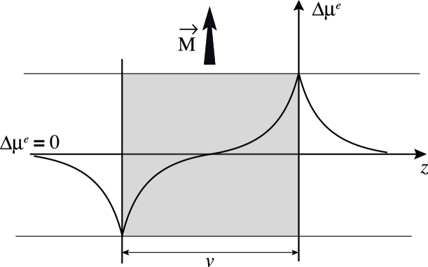
Figure 1: Illustration of the spin-accumulation occurring in a nanoscopic ferromagnetic layer with its two non-ferromagnetic contacts: the profile of the electrochemical potential difference $\Delta\mu^{e}$ is plotted as a function the spatial coordinate $z$.

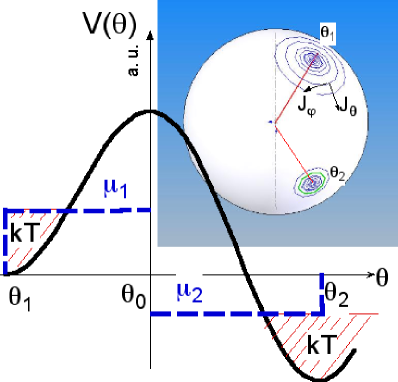
Figure 2: The configuration space of the ferromagnetic order parameter is represented by a sphere of radius unity. The double well shown is a projection over the plane that contains the two equilibrium states at $\theta_{1}$ and $\theta_{2}$, and the top of the barrier at $\theta_{0}$. The step approximation for the chemical potential $\mu(\theta)$ is plotted with the thermal fluctuations sketched by the dashed area around the two minima.

In the presence of spin injection, $\Delta\mu\neq 0$ and a correction to the above LLG equation is expected, due to the phenomenological transport spin-transfer coefficient $l$, introduced in the Onsager matrix of Eq. (2). For the sake of simplicity, we only treat the coupling of longitudinal spin relaxation along the vector $\vec{u}_{\theta}$.

Assuming $l$ constant, the longitudinal component of the total ferromagnetic current in the layer $\vec{\mathcal{J}}^{F}(\theta,\varphi,v)=\int_{v}\vec{j}^{F}(\theta,\varphi,z)dz$ has the form,

$$\mathcal{J}^{\theta F}(\theta,\varphi,v)=j_{0}^{\theta F}(\theta,\varphi)v-l\int_{v}\,\frac{\partial\Delta\mu^{e}}{\partial z}(\theta,z)dz$$ (6)

The quantity $\beta\,\int_{v}\frac{\partial\Delta\mu^{e}}{\partial z}dz$ is proportional to the giant magnetoresistance $R_{GMR}$ generated at the interface ValetFert ; Revue (see Fig. 1 and condition ):

$$\beta\,\int_{v}\frac{\partial\Delta\mu^{e}}{\partial z}dz=8eIR_{GMR}(\theta)$$ (7)

where $J^{e}_{0}=I$ is the electric current injected in the junction of section unity. Since the giant magnetoresistance $R_{GMR}(\theta)$ depends on the angle between the incident spin-polarized current (e.g. defined by the magnetization state of a second magnetic layer in a spin-valve structure) and the ferromagnetic layer, it depends on the state of the ferromagnetic layer, i.e. the position in the $\gamma$-space. Eq. (6) shows that the total ferromagnetic current is simply related to the gradient of a total chemical potential $\mu^{F}_{tot}$:

$$\vec{\mathcal{J}}^{F}=-\bar{\mathcal{L}}\vec{\nabla}\mu^{F}_{tot}$$ (8)

The total chemical potential $\mu^{F}_{tot}$ writes:

$$\mu^{F}_{tot}(\theta)=\mu^{F}(\theta)+\frac{l}{L_{\theta\theta}}\,\mathcal{V}^{e}(\theta)$$ (9)

where the electrospin chemical potential $\mathcal{V}^{e}(\theta)$ is given by an integration over the length of the ferromagnet in the direction $z$, and over the angle $\theta$:

$$\mathcal{V}^{e}(\theta)=\frac{1}{e}\int_{\theta}\int_{v}\frac{\partial\Delta\mu^{e}}{\partial z}(z,\theta^{\prime})dz\,d\theta^{\prime}=\frac{8eI}{\beta}\int_{\theta}R_{GMR}(\theta^{\prime})d\theta^{\prime}$$ (10)

Inserting the ferromagnetic chemical potential Eq. (4) into Eq. (9) yields

$$\mu^{F}_{tot}(\theta)=kT\,ln(\rho_{0}^{F}\left(\theta)\right)+\frac{l}{L_{\theta\theta}}\,\mathcal{V}^{e}(\theta)+vV^{F}(\theta)$$ (11)

In order to deal with the density of the total system $\rho_{tot}^{F}$, the contribution of the spin-dependent scattering is included in the logarithm :

$\mu^{F}_{tot}=kT\,ln(\rho_{tot}^{F})+vV^{F}$ where

$$\rho^{F}_{tot}(\theta)=\rho_{0}^{F}(\theta).e^{\frac{l}{kTL_{\theta\theta}}\,\mathcal{V}^{e}(\theta)}$$ (12)

Consequently, the expression of the ferromagnetic-electrochemical potential takes the same form as in the case of a ferromagnetic chemical potential without spin-injection, but with a modified density (that depends on the spin dependent scattering process).

The total ferromagnetic current, given by Eq. (8), writes now:

$$\vec{\mathcal{J}^{F}}=-\frac{\rho_{tot}^{F}\Gamma}{M_{s}(1+\alpha^{2})}\left\{\vec{u}_{r}\times\left(\vec{\nabla}V^{F}+\frac{k_{B}T}{v}\frac{\vec{\nabla}\rho_{tot}^{F}}{\rho_{tot}^{F}}\right)-\alpha\vec{u}_{r}\times\left[\vec{u}_{r}\times\left(\vec{\nabla}V^{F}+\frac{k_{B}T}{v}\frac{\vec{\nabla}\rho_{tot}^{F}}{\rho_{tot}^{F}}\right)\right]\right\}$$ (13)

Once again, the corresponding generalized LLG equation is directly obtained from the expression $\frac{d\vec{u}_{r}}{dt}=\frac{\vec{\mathcal{J}}_{tot}^{F}}{\rho^{F}_{tot}}$. The equation can be rewritten with introducing the ”pseudo” effective field $\vec{\tilde{H}}_{eff}=-\vec{\nabla}V^{F}+\frac{k_{B}T}{v}\frac{\vec{\nabla}\rho_{tot}^{F}}{\rho_{tot}^{F}}$, so that the Generalized LLG equation takes the usual form:

$$\frac{d\vec{u}_{r}}{dt}=\frac{\Gamma}{M_{s}(1+\alpha^{2})}\left\{\vec{u}_{r}\times\vec{\tilde{H}}_{eff}-\alpha\vec{u}_{r}\times\left[\vec{u}_{r}\times\vec{\tilde{H}}_{eff}\right]\right\}$$ (14)

This equation has the same form than that of the LLG equation without spin-injection (note that it is mainly a consequence of the approximation of longitudinal coupling only, disregarding precessional coupling), but the diffusion part of the effective field is modified through the correction of the density $\rho_{tot}^{F}=\rho_{0}^{F}e^{\frac{l}{k_{B}TL_{\theta\theta}}\mathcal{V}^{e}}$ :

$$k_{B}T\left(\frac{\vec{\nabla}\rho_{tot}^{F}}{\rho_{tot}^{F}}-\frac{\vec{\nabla}\rho_{0}^{F}}{\rho_{0}^{F}}\right)=\frac{l}{L_{\theta\theta}}\frac{\partial\mathcal{V}^{e}}{\partial\theta}\vec{u}_{\theta}$$ (15)

the correction due to spin-injection $\frac{8le}{\beta k_{B}TL_{\theta\theta}v}R_{GMR}I$ is consequently a correction to the diffusion term that is proportional to the GMR and to the injected current. However, this diffusion term accounts for fluctuations Brown . The effect of the diffusion terms cannot be taken into account in the quasi-static hysteresis loop (i.e. for vanishing temperature or infinite measurement times) as a deterministic effective field (this point is discussed in the references Moi ; Revue ). A deterministic correction to the reversible part of the hysteresis (the quasi-static states) is hence not expected here. In contrast, the effect of this correction is considerable in the activation regime or in ferromagnetic resonance near equilibrium, described in the next sections.

.2 Spin-injection correction to the activation process

What is the consequence of the diffusion correction Eq. (15) in the activation regime of magnetization reversal? This question is investigated below for large time scales (beyond nanosecond time scales, or ”high barriers”), with the corresponding activation process, i.e. the so-called Néel-Brown relaxation SpinTorque . In the activation regime, the effect of the precession can be neglected: the gradient $\vec{\nabla}$ and the divergence operator can be reduced to the scalar derivative $\frac{\partial}{\partial\theta}$.

The ferromagnetic potential $V^{F}$ has a double well structure (Fig. 2), with the two minima $\theta_{1}$ and $\theta_{2}$, and a maximum at $\theta_{0}$. The description of the activation process is based on the high barrier approximation under which the ferromagnetic current becomes a step function in the $\theta$ space:

$$\mathcal{J}^{F}(\theta,t)=\mathcal{J}^{F}(t)\left[\Theta(\theta-\theta_{1})-\Theta(\theta-\theta_{2})\right]$$ (16)

where $\Theta(\theta)$ is the Heaviside step function.

The chemical potential can also be approximated by a step function that takes the value of the equilibrium states in the left ($\theta_{1}$) or in the right ($\theta_{2}$) side of the potential barrier in the ferromagnetic configuration space (Fig. 2) : $\mu^{F}(\theta,t)=\mu^{F}(\theta_{1},t)\Theta(\theta_{0}-\theta)+\mu^{F}(\theta_{2},t)\Theta(\theta-\theta_{0})$. Using now this expression, the density function $\rho_{tot}^{F}(\theta)$ of the ferromagnet in configuration space writes:

$$\rho_{tot}^{F}(\theta,t)=\rho_{tot}^{F}(\theta_{1},t)e^{-\frac{v\left(V^{F}(\theta)-V^{F}(\theta_{1})\right)}{k_{B}T}}\Theta(\theta_{0}-\theta)+\rho_{tot}^{F}(\theta_{2},t)e^{-\frac{v\left(V^{F}(\theta)-V^{F}(\theta_{2})\right)}{k_{B}T}}\Theta(\theta-\theta_{0})$$ (17)

The ferromagnetic current is related to the gradient of the generalized chemical potential through our fundamental relation Eq. (8) : $\mathcal{J}^{F}(\theta,t)=-L_{\theta\theta}\frac{\partial{\mu_{tot}^{F}(\theta,t)}}{\partial{\theta}}$. This equation can be written into the more convenient form

$$\mathcal{J}^{F}(\theta,t)=-D_{tot}^{F}(\theta)\,e^{-\frac{vV^{F}(\theta)}{k_{B}T}}\,\frac{\partial e^{\frac{\mu^{F}_{tot}(\theta,t)}{k_{B}T}}}{\partial\theta}$$ (18)

with the diffusion coefficient

$$D_{tot}^{F}(\theta)\equiv\frac{kTL_{\theta\theta}}{\rho_{tot}^{F}(\theta)}=D_{0}^{F}.e^{-\frac{l\mathcal{V}^{e}(\theta)}{k_{B}TL_{\theta\theta}}}$$ (19)

where the second equality is deduced from Eq. (12 ) and the parameter $D_{0}^{F}=L_{\theta\theta}.k_{B}T/\rho_{0}^{F}$ (dimension of angle per unit of time) is the usual ferromagnetic diffusion coefficient that is constant.

The activation process is described by a rate equation (see Eq. (23) below), e. i. a contracted description that is obtained by performing a reduction of the continuous internal variable $\theta$ over the equilibrium states $\theta_{i}$ ($i=\{1,2\}$).

The total flow has a zero divergence current density $div\mathcal{J}^{F}=0$. The system is quasi stationary and the total current is $\mathcal{I}=2\pi sin(\theta)\mathcal{J}(t)$. Eqs. (16) and Eqs. (18) can be integrated over the measure $exp(vV/k_{B}T)d\theta$ to give:

$$\mathcal{I}\int\frac{e^{\frac{vV^{F}(\theta)}{k_{B}T}}}{2\pi sin\theta}\left[\Theta(\theta_{1}-\theta)-\Theta(\theta_{2}-\theta)\right]d\theta=-\int D_{tot}^{F}(\theta)\,e^{-\frac{vV^{F}(\theta)}{k_{B}T}}\,\frac{\partial e^{\frac{\mu^{F}(\theta)}{k_{B}T}}}{\partial\theta}d\theta$$ (20)

so that the total current writes RqueDistrib :

$$\mathcal{I}=D_{tot}^{F}(\theta_{0})\frac{e^{\mu(\theta_{2})/k_{B}T}-e^{\mu(\theta_{1})/k_{B}T}}{\int^{\theta_{2}}_{\theta_{1}}\frac{e^{vV^{F}(\theta)/k_{B}T}}{2\pi\,sin(\theta)}\,d\theta}$$ (21)

Defining the number of representative points near equilibrium by $n(\theta_{i})=\int_{-\epsilon}^{\theta_{i}+\epsilon}\rho(\theta^{\prime})2\pi sin(\theta^{\prime})d\theta^{\prime}$, the density in the double well potential Eq. (17) leads to the expressions:

$$e^{\mu(\theta_{1})/k_{B}T}=\frac{n_{tot}(\theta_{1})}{2\pi\int_{-\epsilon}^{\theta_{0}}e^{-vV^{F}(\theta)/k_{B}T}sin(\theta)d\theta}$$

$$e^{\mu(\theta_{2})/k_{B}T}=\frac{n_{tot}(\theta_{2})}{2\pi\int_{\theta_{0}}^{\theta_{2}+\epsilon}e^{-vV^{F}(\theta)/k_{B}T}sin(\theta)d\theta}$$ (22)

where $\epsilon$ is a real number. Inserting the above equation into Eq. (21) leads to the generalized rate equation:

$$\mathcal{I}=\dot{n}_{tot}(\theta_{1})=-\dot{n}_{tot}(\theta_{2})=\frac{n_{tot}(\theta_{1})}{\tilde{\tau}_{1\rightarrow 2}}-\frac{n_{tot}(\theta_{2})}{\tilde{\tau}_{2\rightarrow 1}}$$ (23)

Using the steepest descents approximation RqueSteepest for the three integrals present in Eq. (21) after inserting Eqs. (22), the total relaxation times write:

$$\tilde{\tau}_{i\rightarrow i\pm 1}^{-1}=D_{tot}(\theta_{0})\frac{sin(\theta_{0})}{sin(\theta_{i})}\frac{v\sqrt{|(V^{F})^{\prime\prime}(\theta_{0})||(V^{F})^{\prime\prime}(\theta_{i})|}}{2\pi kT}e^{\frac{vV^{F}(\theta_{i})-vV^{F}(\theta_{0})}{k_{B}T}}$$ (24)

More explicitly, this generalized rate equation as the form of the usual Néel -Brown relaxation rates $\tau_{i\rightarrow i\pm 1}$, with an exponential correction expressed in terms of the electrospin chemical potential $\mathcal{V}^{e}(\theta_{i})$:

$$\dot{n}_{tot}(\theta_{1})=-\dot{n}_{tot}(\theta_{2})=\frac{n(\theta_{1})}{\tau_{1\rightarrow 2}}e^{-\frac{l\left(\mathcal{V}^{e}(\theta_{1})-\mathcal{V}^{e}(\theta_{0})\right)}{k_{B}T\,L_{\theta\theta}}}-\frac{n(\theta_{2})}{\tau_{2\rightarrow 1}}e^{-\frac{l\left(\mathcal{V}^{e}(\theta_{2})-\mathcal{V}^{e}(\theta_{0})\right)}{k_{B}T\,L_{\theta\theta}}}$$ (25)

where $\mathcal{V}^{e}(\theta)=8eI\int_{0}^{\theta}R_{GMR}(\theta^{\prime})d\theta^{\prime}/\beta$. Accordingly, the Néel-Brown activation law is still valid under current injection, with a correction that can be added to the potential energy barrier. The total potential energy including the contribution of the spin-injection writes :

$$V_{tot}(\theta)=V^{F}(\theta)+\frac{8leI}{\beta L_{\theta\theta}}\int_{\theta}R_{GMR}(\theta^{\prime})d\theta^{\prime}$$ (26)

The correction to the energy barrier is proportional to the current I and to the GMR integrated over the magnetization states corresponding to the energy barrier height. Eq. (25) shows that the process follows the Néel-Brown activation law with the relaxation times: $\tilde{\tau}=\tau_{0}\,e^{-\frac{\Delta V_{tot}}{k_{B}T}}$ where $\Delta V_{tot}=V_{tot}(\theta_{i})-V_{tot}(\theta_{0})$, $\theta_{i}=\{\theta_{1},\theta_{2}\}$ and $\tau_{0}$ is the usual waiting time (i.e. the prefactor in Eq.(24) ).

In order to compare this analysis with experimental results performed on nanopillars, let us assume a spin-valve structure with two ferromagnetic layers composed of identical materials with $\beta\geq 0$, in which only two states along the anisotropy axes are allowed. One layer is fixed (the pinned layer) and the states of the other (the ”free” layer) are investigated. The magnetization states of the free layer are $\theta_{1}=0$ for the parallel configuration (P) and $\theta_{2}=\pi$ for the ant parallel configuration (AP). The GMR for the P state $R_{GMR}(0)=0$ corresponds to the reference configuration (no spin-flip). The AP configuration $R_{GMR}(\pi)=\Delta R$ corresponds to the maximum GMR. If we take the most simple form for the angular dependence of the GMR Dieny $R_{GMR}(\theta)=\Delta R\,\left(1-cos(\theta)\right)$, we have $\mathcal{V}^{e}(0)-\mathcal{V}^{e}(\pi/2)=-\frac{4I\Delta R(\pi-2)}{\beta}$ and $\mathcal{V}^{e}(\pi)-\mathcal{V}^{e}(\pi/2)=+\frac{4I\Delta R(\pi+2)}{\beta}$.

Note that the GMR parameter $\Delta R$ is a function of $\beta$: expressed in terms of the spin diffusion length $l_{sf}$ it writes Revue $\Delta R/R=\frac{\beta^{2}}{1-\beta}\frac{l_{sf}}{v}$ (where $v$ is the length of the layer).

In conclusion, the injection of the current leads to suppress one transition and to accelerate the other: the current provokes the magnetization reversal from one configuration to the other, and the transition depends on the current direction. In the exemple ebove, the current provokes the magnetization reversal from P to AP configuration for positive current, and provokes the magnetization reversal from AP to P configuration for negative current. This is a sufficient condition in order to accounts for the hysteresis loop of the magnetization driven by the current. In the general case, both transitions are defined with the relaxation rate

$$\tau_{i}=\tau_{0}\,e^{-\frac{\Delta V^{F}\pm\frac{c_{i}\,l\Delta R}{\beta L_{\theta\theta}}I}{2k_{B}T}}$$ (27)

with a asymmetry factor $c_{i}\equiv\int_{\theta_{i}}^{\theta_{0}}R_{GMR}(\theta)d\theta/\Delta R$, and the coefficient $L_{\theta,\theta}$ is defined in Eq. (3)

( $c_{P}=(\pi-2)/2$ and $c_{AP}=(\pi+2)/2$ in the simple exemple given above). The quasi-symmetry under both the permutation of the magnetic configurations and the change of the current direction observed experimentally is hence contained in the result expressed in Eq. (25).

From an empirical point of view, the expression often used in order to fit the data introduces the critical current $I_{c}$ (measured at zero external field and extrapolated at zero Kelvin), such that: $\tilde{\tau}=\tau_{0}\,e^{-\frac{E_{a}}{kT}(1-\frac{I}{I_{c}})}$ where $E_{a}$ is the anisotropy energy of the ferromagnetic layer under consideration. Result Eq. (25) shows that the critical current is given by the expression:

$$I_{c}=-\frac{\Gamma\alpha E_{a}}{vM_{s}(1+\alpha^{2})c_{i}}\left(\frac{\rho^{F}_{0}}{el}\right)\frac{\beta}{8\Delta R}$$ (28)

The Néel-Brown law under current injection is measured in references MSU2 ; Moi ; Fabian ; Buhrman , with the typical asymmetry between the two transitions of a factor 2 to 4. The relation $I_{c}\propto 1/\Delta R$ is verified in reference MSU2 . The proportionality with $\beta$ is observed through the change of the sign while changing the scattering anisotropy MSU3 . Note that the phenomenological results presented here can be generalized to tunnel junctions (see e.g. the work of Schmidt and et al. in terms of spin injection in magnetic semiconductors Molenkamp ). In the case of tunnel barrier a factor ten is typically gained in the magnetoresistance $\Delta R$, so that the critical currents in Eq. (28) are also decreased by a factor ten TJ .

What is the value of the spin-transfer coefficient $l$? In order to compare with the ferromagnetic transport coefficient $L_{\theta\theta}/\rho_{0}^{F}=\Gamma\alpha/(M_{s}(1+\alpha^{2}))$ - expressed as the inverse of an action $J^{-1}.s^{-1}$ - the phenomenological coefficient is compared in the same units: $\frac{l}{e\rho_{0}^{F}}=-\frac{E_{a}\beta}{e8\Delta RI_{c}c_{i}}\left(\frac{L_{\theta\theta}}{\rho_{0}^{F}}\right)$.

Experiments performed on typical pseudo spin-valve systems show that it is possible to switch the magnetization at zero external field in both directions (AP to P or P to AP in the previous exempla) for currents of the order of $\pm$ 1 mA. For such currents, the energy transferred is of the order of 10 meV MSU2 : the measured quantity is the slope of the points $1/I_{c}$ plotted as a function of $\Delta R$ for the two transitions. The anisotropy energy $E_{a}$ is of the order of 0.1 $eV$. The spin-transfer coefficient $l/e$ is consequently of the order of $10^{-1}L_{\theta\theta}$ to $10^{-2}L_{\theta\theta}$.

On the other hand, the activation experiments under current injection allow to access directly to the spin-transfer coefficient through the Néel-Brown law, without the need to measure the activation energy $E_{a}$. The quantity measured is the slope $s=\partial(ln(\tau/\tau_{0}))/\partial I$. Eq. (26) and Eq. (27) show that: $\frac{l}{eL_{\theta\theta}}=kTs\beta\left(8e\int_{\theta_{eq}}^{\theta_{0}}R_{GMR}(\theta^{\prime})d\theta^{\prime}\right)^{-1}\approx 0.1$. The order of magnitude $10^{-1}$ is confirmed experimentally in references MSU2 ; Moi , together with the factor 2 to 4 in the asymmetry.

.3 Spin-injection correction to the fluctuations

Due to its diffusive nature, the correction produced by the spin-injection can hardly be observed on the reversible state of the hysteresis. The above section shows that the activated irreversible jump of the magnetization is in contrast strongly modified by the spin-injection. Beyond the activation process, the presence of supplementary ferromagnetic diffusion processes strongly affects another experimentally accessible parameter: the linear response of the ferromagnetic moment to magnetic field, spin-injection, and thermal excitations. The response is then proportional to the fluctuations.

The fluctuations occurring near the quasi-static states in the double-well potential can be analyzed from the general fluctuation-dissipation theorem (FDT) in the $\gamma$-space RubiFDT . The density $\tilde{\rho}^{F}$ is subjected to random fluctuations that are introduced through a random current $\mathcal{J}_{r}^{F}$, which satisfies FDT:

$$\langle\mathcal{J}^{F}_{r}(\theta,t)\mathcal{J}_{r}(\theta^{\prime},t^{\prime})\rangle=2D_{tot}^{F}(\theta)\langle\rho_{tot}^{F}(\theta,t)\rangle\delta(\theta-\theta^{\prime})\delta(t-t^{\prime})$$ (29)

The variation of density is now corrected by the presence of the fluctuation current:

$$\frac{\partial}{\partial t}\rho_{tot}(\theta,t)=-\mathcal{J}^{F}(\theta,t)-\mathcal{J}_{r}^{F}(\theta,t)$$ (30)

Applying step by step the method described above for the rate equation (Eqs. (20) to (23)) to the Eq. (30) , the following expression of the fluctuations is obtained (see reference RubiFDT ):

$$\langle\mathcal{I}_{r}(t)\mathcal{I}_{r}(t^{\prime})\rangle=\frac{\langle n_{tot}^{F}\rangle(\theta_{1})}{\tilde{\tau}_{1\rightarrow 2}}-\frac{\langle n_{tot}^{F}\rangle(\theta_{2})}{\tilde{\tau}_{2\rightarrow 1}}$$ (31)

where the relaxation times $\tilde{\tau}$ are that previously defined. This expression has not the usual form of a FDT which means that this theorem, strictly valid when fluctuations take place around equilibrium states, is not fulfilled. The theorem is restored near an equilibrium state $\langle n_{tot}^{F}\rangle^{eq}=\langle n_{tot}^{F}\rangle(\theta_{1})$ or $\langle n_{tot}^{F}\rangle^{eq}=\langle n_{tot}^{F}\rangle(\theta_{2})$ because transitions from one equilibrium state to the other are neglected. We obtain from Eq. (31) $\langle\mathcal{I}_{r}(t)\mathcal{I}_{r}(t^{\prime})\rangle^{eq}=\frac{\langle n_{tot}^{F}\rangle^{eq}}{\tilde{\tau}_{eq}}\delta(t-t^{\prime})$. This last expression is valid in the cases of linear ferromagnetic resonance experiments, i.e. in a situation where the current is well below the critical current $I_{c}$ defined in Eq. (28) DienyRes . A more complicated behavior (highly non-linear) should be expected for strong excitations near or beyond the critical current $I_{c}$ in order to interpret the non-linear resonance experiments STReson .

In conclusion, in the case of linear ferromagnetic resonance (FMR) measured below $I_{c}$ and observed close to one equilibrium state ($\theta_{1}$ or $\theta_{2}$), a correction to the response of the ferromagnet is expected, that takes the same form as that calculated for the activation process:

$$\langle\mathcal{I}_{r}(t)\mathcal{I}_{r}(t^{\prime})\rangle^{eq}=2D_{0}^{F}\,\frac{\langle n_{0}^{F}\rangle}{\tau_{eq}}exp\left(-\frac{l(\mathcal{V}^{e}(\theta_{i})-\mathcal{V}^{e}(\theta_{0}))}{k_{B}T\,L_{\theta\theta}}\right)\delta(t-t^{\prime})$$ (32)

The behavior expected is then surprisingly similar to that predicted in the case of the activation process, except that it holds for the amplitude of the linear response and not for the transition rates. For $\beta\geq 0$, we expect an exponential increase (resp. suppression) of the response in the AP state with a positive (resp. negative) current, and an exponential increase (resp. suppression) of the response in the P state with a negative (resp. positive) current. This highly specific characteristic is in agreement with that observed experimentally in the context of FMR measurements under spin-injection below critical current $I_{c}$, i.e. a situation in which the magnetization is close enough to equilibrium states (see results presented in reference DienyRes ).

.4 Link with microscopic theories

Before concluding, a last question must be invoked about the relation between the model presented here and the microscopic theories of spin-transfer torque Slon ; Berger ; Miltat ; ListTheo . The phenomenological transport coefficient $l$ (and of course the known transport coefficient $L_{\theta\theta}$ and $\beta\sigma_{0}$) could formally be defined from the relevant Hamiltonian expression with the help of projection-operator formalisms Fick , or any other techniques Kambersky ; Montigny that lead to the coupled stochastic transport equations of the spin-polarized current and the ferromagnetic order parameter in the corresponding configuration space. The difficulty is to manipulate on an equal footing a microscopic degree of freedom, the spin of conduction electrons, and a collective variable, the magnetic order parameter. This task is far beyond the present report, but it is possible to gain some insight with dimension considerations. The physical mechanism proposed here for spin-transfer is based on the spin-injection only, that is responsible for the supplementary diffusion effect of the magnetization through the modification of the local densities of magnetic moments (redistribution of spins). This redistribution of spins between the electric sub-system and the magnetic sub-system is governed by specific spin-flip scattering mechanisms (or spin dependent creation-anhilation mechanisms). The microscopic approach would define the relevant mechanism and deduce the typical spin-transfer relaxation time $\tau_{tr}$. The relation between mesoscopic and microscopic approaches can consequently be invoked through the relation between the correction of the diffusion constant $\delta D_{tot}^{F}$ (expressed in dimension of angle per unit of time) and the relaxation time: $\delta D_{tot}^{F}\propto\delta n/\tau_{tr}$, where $\delta n$ is the amount of spins transferred from the electric sub-system to the ferromagnet.

In the approach proposed by Berger Berger in a pioneering work, a spin-transfer process at the interface is described at the electronic level by a typical spin relaxation time $\tau_{sd}$ calculated from the s-d exchange Hamiltonian. If we assuming that the relevant spin-flip relaxation is governed by this mechanism $\tau_{tr}=\tau_{sd}$, we would have $\delta D_{tot}^{F}\propto 1/\tau_{sd}$ under the relevant hypotheses. In that case, the spin-transfer described here in terms of diffusion process would be a consequence, in parallel to GMR effects, of the s-d exchange interaction occuring at the microscopic level.

.5 Conclusion

A description of spin-transfer has been proposed at the mesoscopic level, based uniquely on the spin-injection mechanism occuring at the junction with a ferromagnet. The spin-accumulation at the interface leads to a local change of the density of magnetic moments in the corresponding configuration space. The gradient of density generates a diffusion process of the ferromagnetic order parameter, which is responsible for the magnetization reversal.

The spin-injection has been described at the interface of a ferromagnet by means of the usual two-conduction channel model which simplifies the spin-polarized current and the giant magnetoresistance analyses. The dynamics of the ferromagnet is treated by means of an out-of-equilibrium mesoscopic model with a ferromagnetic current defined in the configuration space of uniform magnetic moments. The coupling between the two currents is introduced through a new phenomenological Onsager cross-coefficient $l$ that accounts for the fact that the spins carried by the electric charges in the normal space contribute also to the transport of ferromagnetic moments in the ferromagnetic configuration space. It as been shown that the correction to the LLG equation that governs the dynamic of the magnetization comes from a diffusion term. We have found that the Néel-Brown activation law is still valid, with a correction to the barrier height that is proportional to the integral of the giant magnetoresistances over the ferromagnetic states, from the equilibrium to the top of the barrier. The expression of the critical current $I_{c}$ is given as a function of GMR, the damping factor and the new spin-transfer cross-coefficient $l$. Furthermore, the correction to the fluctuations is shown to be analogous to that of the activation and is also expressed as an exponential term. These results are consistent with the results obtained experimentally in quasi-static modes (hysteresis loops as a function of the current), in the activation regime under spin-injection, and in linear resonance experiments under spin-injection with $I\leq I_{c}$.

References

- (1) M. Tsoi et al. Phys. Rev. Lett. 80, 4281 (1998), J-E. Wegrowe et al. Europhysics lett. 45 626 (1999), F. J. Albertet al. Appl. Phys. Lett. 77 3809 (2000), J. Grollier et al. Appl. Phys. Lett. 78, 3663 (2001), E. B. Myers et al. Phys. Rev. Lett. 89, 196801 (2002), J. Z. Sunet al. Appl. Phys. Lett. 81, 2202 (2002), J.-E. Wegrowe et al. Appl. Phys. Lett. 80, 3775 (2002), B. Oezyilmazet al. Phys. Rev. Lett 91, 067203 (2003).
- (2) ”A Novel Nonvolatile Memory with Spin Torque Transfer Magnetization Switching: Spin-RAM” ; M. Hosomi et al. IEDM Technical Digest. IEEE International, 459 (2005).
- (3) M. N. Baibich, J. M. Broto, A. Fert, F. Ngyen Van Dau, F. Petroff, P. Etienne, G. Creuzet, A. Friederich, and J. Chazelas, Phys. Rev. Lett. 61, 2472 (1988) and G. Binasch, P. Grunberg, F. Saurenbach, and W. Zinn, Phys. Rev. B 39, 4828 (1989).
- (4) M. Johnson and R.H. Silsbee Phys. Rev. B 35, 4959 (1987); M. Johnson and R. H. Silsbee, Phys. Rev. B 37, 5312 (1988).
- (5) P. C. van Son, H. van Kempen, and P. Wyder, Phys. Rev Lett. 58, 2271 (1987).
- (6) T. Valet and A. Fert, Phys. Rev. B, 48, 7099 (1993).
- (7) P. M. Levy, H. E. Camblong, S. Zhang, J. Appl. Phys. 75, 7076 (1994).
- (8) J.-E. Wegrowe, Phys. Rev. B 62, 1067 (2000).
- (9) D. Reguera, J. M. Rubí, and J. M. G. Vilar, J. Phys. Chem. B 109 (2005) 21502.
- (10) A. Perez-Madrid, D. Reguera, J.M. Rubí, Physica A 329 (2003), 357.
- (11) J. C. Slonczewski, J. Magn. Magn. Mat. 159 L1 (1996).
- (12) L. Berger Phys. Rev. B 54, 9353 (1996).
- (13) M. Stiles and J. Miltat in Spin Dynamics in confined Magnetic Structures III, Ed. B. Hillebrands, and A. Thiaville (Springer, Berlin 2006).
- (14) J.-E. Wegrowe, M. C. Ciornei, H.-J. Drouhin, J. Phys.: Condens. Matter 19, 165213 (2007).
- (15) S. Urazhdin, O. Norman, W. Birge, W. P. Pratt, and J. Bass, Phys. Rev. Lett. 92, 146803 (2003) and M. AlHajDarwish, A. Fert, W. P. Pratt Jr. and J. Bass J. Appl. Phys. 95, 7429 (2004).
- (16) Y. Jiang, S. Abe, T. Ochiai, T. Nozaki, A. Hirohata, N. Tezuka, and K. Inomata, Phys. Rev. Lett. 92, 167204 (2004).
- (17) A. Manchon, N. Strelkov, A. Deac, A. Vedyayev, and B. Dieny, Phys. Rev. B 73, 184418 (2006).
- (18) J.-E. Wegrowe, Phys. Rev. B 68, 214414 (2003)
- (19) A. Fabian, C. Terrier, S. Serrano Guisan, X. Hoffer, M. Dubey, L. Gravier, J.-Ph. Ansermet, and J.-E. Wegrowe, Phys. Rev. Lett. 91, 257209 (2003).
- (20) I. N. Krivorotov, N. C. Emley, A. G. F. Garcia, J.C. Sankey, S. I. Kiselev, D. C. Ralph, and R. A. Buhrman, Phys. Rev. Lett. 93, 166603 (2004).
- (21) S. Petit, C. Baraduc, C. Thirion, U. Ebels, Y. Liu, M. Li, P.Wang, and B. Dieny, Phys. Rev. Lett. 98, 077203 (2007).
- (22) J.-E. Wegrowe, Q. Anh Nguyen, M. Al-Barki, J.-F. Dayen, T. L. Wade, and H.-J. Drouhin, Phys. Rev. B 73 134422, (2006).
- (23) The -space is the space of the ”internal degree of freedom”, as defined by Ilya Prigogine and Peter Mazur in Physica 19, 241 (1953).
- (24) The discussion about the definition of the generalized flux (and typically about the heat current) from the entropy production can be found in S. R. De Groot and P. Mazur, non equilibrium thermodynamics Amsterdam : North-Holland, 1962. See also the discussion in the context of transport in semiconductors by J. E. Parrott, IEEE Trans. Electron Devices 43, 809 (1996).
- (25) For a first principle approach, see E.C.G. Stueckelberg and P.B. Scheurer, thermocinétique phénoménologique galiléenne” Birkauser Verlag, Basel and Stuttgart, 1974.
- (26) A statistical justification of this typical form of the chemical potential was given by P. Mazur, Physica A 261, 451 (1998).
- (27) See the discussion for the introduction of the diffusion term by Brown Jr. in W. F. Brown Jr., Phys. Rev. 130, 677 (1963)
- (28) S. Urazhdin, N. O. Birge, W. P Pratt, J. Bass, Appl. Phys. Lett. 84, 1516 (2004).
- (29) In the framework of the two channel approximation (with channels and ), an interface between two layers of length and , conductance and , and spin-diffusion length and gives rise to the resistance: , as derived in Wegrowe et al. J. Phys.: Condens. Matter 19, 165213 (2007).
- (30) This approach cannot be identified, without further considerations, to the derivation of an activation process under spin-transfer-torque, provoked by a deterministic spin-torque term added to the Landau-Lifshitz-Gilbert equation (in our case, the derivation is based on the diffusion term). Such studies with spin-transfer torque can be found in Z. Li and S. Zhang, Phys. Rev.B 69 134416 (2004), D. M. Apalkov and P. B. Visscher, Phys. Rev. B, 72 180405(R) (2005), C. Serpico, G. Bertotti, I. D. Mayergoyz, M. d’Aquino, R. Bonin, J. Appl. Phys. 99, 08G505 (2006) and G. Bertotti, C. Serpico, I. D. Mayergoyz, R. Bonin, M. d’Aquino, J. Mag. Magn. Magn. 316 285 (2007).
- (31) B. Dieny, V. S. Seriosu, S. S. P. Parkin, B. A. Gurney, D. R. Wilhoit, D. Mauri, Phys. Rev. B 43, 1297 (1991).
- (32) According to the expression of the chemical potential in terms of Heaviside distributions, the derivative in the sense of the distribution of is where is the Dirac distribution.
- (33) The Steepest step Descent approximation writes: where is a twice-differentiable function with a global maximum in and M is a large number compared to .
- (34) G. Schmidt, D. Ferrand, L. W. Molenkamp, A. T. Filip, and B. J. van Wees, Phys. Rev. B 62, R4790 (2000).
- (35) Yiming Huai et al. Appl. Phys. Lett. 84, 3118 (2004), K. Yagami et al. Appl. Phys. Lett. 85, 5634 (2004), Zhitao Diao et al. Appl/ Phys. Lett. 87, 232502 (2005), Jun Hayakawa et al. Japanese. J. Appl. Phys. 44, L1267 (2005), Zhitao Diao et al. J. Appl. Phys. 99, 08G510 (2006), Hitoshi Kubota et al. Appl. Phys. Lett. 89, 032505 (2006), T. Inokuchi et al. Appl. Phys. Lett. 89, 102502 (2006), G. D. Fuchs et al. Phys. Rev. Lett. 96, 186603 (2006) Z. T. Diao et al. J. Phys.: Condens. Matter 19, 195209 (2007), Masatoshi Yoshikawa et al. J. Appl. Phys. 101, 09A511 (2007).
- (36) S. I. Kiselev et al. Nature 425, 380 (2003)., M. R. Pufall et al. Phys. Rev. B 69, 214409 (2004), M. Covingtonet al. Phys. Rev. B, 69, 184406 (2004), I.N. Krivorotovet al. Science 307 28 (2005), T. Devolderet al. Phys. Rev. B 71, 184401 (2005).
- (37) Ya. B. Bazaliy, B.A. Jones, and S.-C. Zhang, Phys. Rev. B, 57, R3213 (1998), X. Waintal , E. B. Myers, P. W. Brouwer, and D. C. Ralph, Phys. Rev. B 62, 12317 (2000), A. Brataas, Yu. Nazarov, and G.E.W Bauer, Phys. Rev. Lett. 84, 2481 (2000); D. Harnando, Y. V. Nazarov, A. Brataas, and G.E.W Bauer, Phys. Rev. B 62, 5700 (2000); S. Zhang, P. M. Levy, and A. Fert, Phys. Rev. Lett. 88, 236601 (2002), M. D. Stiles, J. X. Xiao, and A. Zangwill, Phys. Rev. B 69, 054408 (2004), M. L. Polianski and P. W. Brouwer, Phys. Rev. Lett. 92, 026602 (2004), J.W. Zhang, P. M. Levy, S.F. Zhang, V. Antropov, Phys. Rev. Lett. 93, 256602 (2004), P. M. Levy and J.W. Zhang, Phys. Rev. B 70, 132406 (2004), J. Barnas, A. Fert, M. Gmitra, I. Weymann, and V. K. Dugaev, Phys. Rev. B 72,024426 (2005).
- (38) E. Fick and S. Sauermann, the quantum statistics of Dynamic Processes, Springer Series in Solid-States Sciences 86, Ed. M. Cardona, P. Fulde, K. von Klitzing, H.-J. Queisser, Berlin Heidelberg 1990.
- (39) V. Kambersky, Can. J. Phys. 48, 2906 (1970), V. L. Safonov and H. N. Bertram, Phys. Rev. B 71, 224402 (2004).
- (40) F. M. Saradzhev, F. C. Khanna, Sang Pyo Kim, M. de Montigny, Phys. Rev. B 75, 024406 (2007).