Tunneling dynamics of few bosons in a double well

Abstract

We study few-boson tunneling in a one-dimensional double well. As we pass from weak interactions to the fermionization limit, the Rabi oscillations first give way to highly delayed pair tunneling (for medium coupling), whereas for very strong correlations multi-band Rabi oscillations emerge. All this is explained on the basis of the exact few-body spectrum and without recourse to the conventional two-mode approximation. Two-body correlations are found essential to the understanding of the different tunnel mechanisms. The investigation is complemented by discussing the effect of skewing the double well, which offers the possibility to access specific tunnel resonances.

I Introduction

Using ultracold atoms, it has become possible to study hallmark quantum effects—such as tunneling—at an unprecedented level of precision and control pitaevskii ; dalfovo99 ; pethick ; leggett01 . One prime example is tunneling of matter waves, where Bose-Einstein condensates have facilitated the observation of Josephson oscillations albiez05 ; milburn97 ; smerzi95 and the complementary nonlinear self-trapping albiez05 ; anker05 ; javanainen86 . In the case of Josephson oscillations, the atoms—initially prepared mostly in one well—simply tunnel back and forth between two potential wells in analogy to a current in a Josephson junction. However, above a critical interaction strength, the atoms essentially remain trapped in that well for the experimental lifetime even though they repel each other.

While the above effects have been observed for macroscopic coherent matter waves, many tools such as optical lattices have promoted a trend to study smaller systems with few atoms only. Permitting a high degree of control, they offer the chance to study finite-size effects and this way allow for a deeper understanding of the microscopic mechanisms in ultracold atoms. As an example, the recently evidenced stability of repulsively interacting atom pairs as they move in a lattice winkler06 , as well as the direct observation of their first- and second-order tunneling dynamics foelling07 , should be seen as few-body counterparts of the above self-trapping transition. This motivates a thorough theoretical investigation of the few-boson tunneling mechanisms.

However, while those effects are confined to the regime of relatively weak interactions, interatomic forces can be adjusted experimentally over a wide range, e.g., by exploiting Feshbach resonances koehler06 . In particular, it is well known that in one dimension (1D) one can tune the effective interaction strength at will via a confinement-induced resonance Olshanii1998a , which makes it possible to explore the limit of strong correlations. If the bosons repel each other infinitely strongly, they can be mapped to noninteracting fermions girardeau60 , in that the exclusion principle serves to mimic the hard-core interaction. While the bosons share local aspects with their fermionic counterparts, nonlocal properties such as their momentum distribution are very different. Sparked also by the experimental demonstration paredes04 ; kinoshita04 ; kinoshita06 , this fermionization has attracted broad interest (see girardeau00 ; das02 ; Busch03 ; minguzzi05 ; alon05 ; deuretzbacher06 ; zoellner06a ; zoellner06b ; zoellner07a and Refs. therein).

In this light, the question naturally arises whether the notion of tunneling can be pushed to the strongly interacting fermionization limit. Indeed, a recent study has shown that a fermionized atom pair tunnels coherently almost like a single atom zoellner07c . In this paper, we give a systematic account of how few-boson tunneling evolves in the crossover from weak to strong correlations. Moreover, we extend that study to two-atom tunneling resonances occuring in asymmetric wells.

Our paper is organized as follows. Section II introduces the model and briefly reviews the concept of fermionization. In Sec. III, we give a concise presentation of the computational method. The subsequent section is devoted to the results on tunneling in a symmetric double well for two atoms (Secs. IV.1–IV.3) and more atoms (Sec. IV.4). Finally, we illuminate the effect of tilting the double well in Sec. V.

II Theoretical background

II.1 Model

The subject of this article is the double-well dynamics of few atoms ($N=2-4$), which shall be described by the many-body Hamiltonian (see zoellner06a for details)

$$H=\sum_{i=1}^{N}\left[\frac{1}{2}p_{i}^{2}+U(x_{i})\right]+g\sum_{i<j}\delta_{\sigma}(x_{i}-x_{j}).$$

Here the double-well trap $U(x)=\frac{1}{2}x^{2}+h\delta_{w}(x)$ is modeled as a superposition of a harmonic oscillator and a central barrier shaped as a Gaussian $\delta_{w}(x)=e^{-x^{2}/2w^{2}}/\sqrt{2\pi}w$ (of width $w=0.5$, where harmonic-oscillator units are employed throughout.) The effective interaction in 1D can be represented as a contact potential Olshanii1998a , but is mollified here with a Gaussian $\delta_{\sigma=0.05}$ so as to alleviate the well-known numerical difficulties caused by the $\delta$ function. We focus on repulsive forces, i.e., $g\in[0,\infty)$.

To prepare the initial state $\Psi(0)$ with a population imbalance—in our case, such that almost all atoms reside in the right well only—we make that side energetically favorable by adding a linear external potential $-d\cdot x$ (with sufficiently large $d\sim 0.1-1$, depending on $N$ and $g$) and let the system relax to its ground state $\Psi_{0}^{(d>0)}$. To study the time evolution in the symmetric double well (Sec. IV), the asymmetry $d$ will be ramped down to $d\to 0$ nonadiabatically (we typically choose a ramp time $\tau\sim 1$). By extension, it is possible to take any final asymmetry $\lim_{t\to\infty}d(t)\neq 0$, which allows us to look at the case where one well is energetically offset (Sec. V).

II.2 Fermionization

A peculiarity of 1D systems is that bosons with infinitely strong repulsive point interactions, $g\to\infty$, become impenetrable. Mathematically, this means that its configuration space becomes disconnected into regions $\{x_{i}\neq x_{j}\>\forall i<j\}$, a feature which allows the system to be solved exactly via the Bose-Fermi map girardeau60 that establishes an isomorphy between the exact bosonic wave function $\Psi_{g\to\infty}^{+}$ and that of a (spin-polarized) non-interacting fermionic solution $\Psi_{0}^{-}$,

$$\Psi_{\infty}^{+}=A\Psi_{0}^{-},$$ (1)

where $A=\prod_{i<j}\mathrm{sgn}(x_{i}-x_{j})$. The mapping rests on general grounds and is valid for both stationary and explicitly time-dependent states. Since $A^{2}=1$, their (diagonal) densities as well as their energy $E$ will coincide with those of the corresponding free fermionic states. That makes it tempting to think of the exclusion principle as mimicking the interaction ($g\to\infty$), which is why this limit is commonly referred to as fermionization.

III Computational method

Our goal is to investigate the few-atom quantum dynamics in the crossover to the highly correlated fermionization limit $g\to\infty$ in an exact fashion. This is numerically challenging, and most studies on the double-well dynamics so far have relied on two-mode models milburn97 ; tonel05 ; salgueiro06 ; creffield07 ; dounasfrazer07a valid for sufficiently weak coupling. Here we adopt the Multi-Configuration Time-Dependent Hartree (mctdh) method mey90:73 ; bec00:1 ; mctdh:package . Its principal idea is to solve the time-dependent Schrödinger equation

$$\begin{array}[]{c}i\dot{\Psi}(t)=H\Psi(t)\end{array}$$

as an initial-value problem by expanding the solution in terms of direct (or Hartree) products $\Phi_{J}\equiv\varphi_{j_{1}}\otimes\cdots\otimes\varphi_{j_{N}}$:

$$\Psi(t)=\sum_{J}A_{J}(t)\Phi_{J}(t).$$ (2)

The (unknown) single-particle functions $\varphi_{j}$ ($j=1,\dots,n$) are in turn represented in a fixed primitive basis implemented on a grid.

Note that in the above expansion not only the coefficients $A_{J}$ but also the single particle functions $\varphi_{j}$ are time dependent. Using the Dirac-Frenkel variational principle, one can derive equations of motion for both $A_{J},\varphi_{j}$ bec00:1 . Integrating this differential-equation system allows us to obtain the time evolution of the system via (2). This has the advantage that the basis $\{\Phi_{J}(t)\}$ is variationally optimal at each time $t$. Thus it can be kept relatively small, rendering the procedure very efficient. We stress that $\Psi$ obeys bosonic permutation symmetry even though the direct-product basis does not; this is ensured by correct symmetrization of the expansion coefficients.

Although designed for time-dependent simulations, it is also possible to apply this approach to stationary states. This is done via the so-called relaxation method kos86:223 . The key idea is to propagate some wave function $\Psi(0)$ by the non-unitary $e^{-H\tau}$ (propagation in imaginary time.) As $\tau\to\infty$, this exponentially damps out any contribution but that stemming from the true ground state like $e^{-(E_{m}-E_{0})\tau}$. In practice, one relies on a more sophisticated scheme termed improved relaxation mey03:251 ; meyer06 , which is much more robust especially for excitations. Here $\langle\Psi|H|\Psi\rangle$ is minimized with respect to both the coefficients $A_{J}$ and the orbitals $\varphi_{j}$. The equations of motion thus obtained are then solved iteratively by first solving for $A_{J}$ with fixed orbitals and then ‘optimizing’ $\varphi_{j}$ by propagating them in imaginary time over a short period. That cycle will then be repeated.

IV Symmetric double well

Let us first focus on the tunnel dynamics in a symmetric well ($d=0$). Our primary focus is on how the tunneling changes as we pass from single-particle—i.e., uncorrelated—tunneling ($g=0$) to tunneling in the presence of correlations and finally to the fermionization limit ($g\to\infty$). It is natural to first look at the conceptually clearest situation where $N=2$ atoms initially reside in the right-hand well (Sec. IV.1), with an eye toward the link between tunneling times and the few-body spectrum (Sec. IV.2) as well as the role of two-body correlations (Sec. IV.3). With this insight, we tackle the more complicated dynamics of $N=3,4,\dots$ atoms in Sec. IV.4.

IV.1 From uncorrelated to pair tunneling

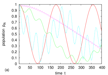
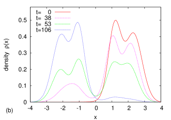
Figure 1: (color online) Two-atom dynamics. (a) Population of the right-hand well over time, $p_{\mathrm{R}}(t)$, for different interaction strengths $g=0$ (—), $g=0.2$ (- - -), $g=4.7$ (${\color[rgb]{1,0,1}\cdots}$), and $g=25$ (${\color[rgb]{0,1,1}-\cdot-}$). (b) Snapshots of the one-body density $\rho(x)$ for different times $t$ in the strongly correlated case $g=25$. (All quantities in harmonic-oscillator units throughout, see text.)

Absent any interactions, the atoms should simply Rabi-oscillate back and forth between both wells. This can be monitored by counting the percentage of atoms in the right well, $p_{\mathrm{R}}(t)=\langle\Theta(x)\rangle_{\Psi(t)}=\int_{0}^{\infty}\rho(x;t)dx$ ($\rho$ being the one-body density) or, correspondingly, the population imbalance $\delta=p_{\mathrm{R}}-p_{\mathrm{L}}=2p_{\mathrm{R}}-1$. Figure 1(a) confirms that $p_{\mathrm{R}}$ harmonically oscillates between 1 and 0. By contrast, if the atoms repel each other, then the tunneling process will be modified. For $g=0.2$, one sees that the tunneling oscillations have become a two-mode process: There is a fast (small-amplitude) oscillation which modulates a much slower oscillation in which the atoms eventually tunnel completely ($p_{\mathrm{R}}\approx 0$). In case $g$ is increased further, we have found that the tunneling period becomes indeed so long that complete tunneling may be hard to observe. For instance, at $g=1.3$ (not displayed here) the period is as large as $2\times 10^{3}$. What remains is a very fast oscillation with only a minute amplitude – this may be understood as the few-body analogue of quantum self-trapping, as will be discussed in Sec. IV.2. As we go over to much stronger couplings (see $g=4.7$), we find that the time evolution becomes more complex, even though this is barely captured in the reduced quantity $p_{\mathrm{R}}$ [Fig. 1(a)]. What is striking, though, is that near the fermionization limit (see $g=25$) again a simple picture emerges: The tunneling, whose period roughly equals that of the Rabi oscillations, is superimposed by a faster, large-amplitude motion. This intriguing result states that the strongly repulsive atoms coherently tunnel back and forth almost like a single particle. As an illustration, snapshots of the density at different $t$ are displayed in Fig. 1(b): At $t=0$, the fragmented pair starts out in the right well, and gradually tunnels to the left well until the fermionized pair state reemerges on the left at $t\approx 106$.

IV.2 Spectral analysis

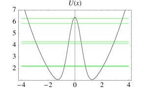
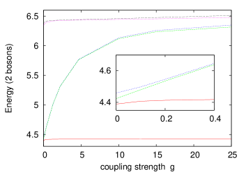
Figure 2: (color online) (a) Single-particle spectrum $\{\epsilon_{a}\}$ of a double well with barrier height $h=8$. (b) Two-particle spectrum as a function of the interaction strength $g$. Inset: Doublet formation with increasing $g$.

In order to understand the oscillations, let us regard the evolution of the few-body spectrum $\{E_{m}(g)\}$ as $g$ is varied (Fig. 2b). In the noninteracting case, the low-lying spectrum of $N=2$ atoms is given by distributing all atoms over the symmetric and antisymmetric single-particle orbital of the lowest doublet (illustrated in Fig. 2a). This yields the $N+1$ energies

$$\{E_{m}=E_{0}+m\Delta^{(0)}\mid m=0,\dots,N\},$$

where $\Delta^{(0)}=\epsilon_{1}-\epsilon_{0}$ is the energy gap between these two orbitals or, in other words, the width of the lowest band. Assuming that for sufficiently small $g$ still only $N+1=3$ levels are populated in $\Psi(t)=\sum_{m}e^{-iE_{m}t}c_{m}\Psi_{m}$, then the imbalance $\delta(t)\equiv\langle\Theta(x)-\Theta(-x)\rangle_{\Psi(t)}$ (and likewise $p_{\mathrm{R}}$) can easily be computed to be

$$\delta(t)=\delta^{\left(01\right)}\cos(\omega_{01}t)+\delta^{\left(12\right)}\cos(\omega_{12}t),$$ (3)

where $\omega_{mn}=E_{m}-E_{n}$ and $\delta^{(mn)}=4\langle\Psi_{m}|\Theta(x)|\Psi_{n}\rangle c_{m}c_{n}$ is determined by the participating many-body eigenstates. Note that the term $(mn)=(02)$ vanishes since, by antisymmetry, only opposite-parity states are coupled. At $g=0$, due to the levels’ equidistance, only a single mode with Rabi frequency $\omega_{01}=\omega_{12}=\Delta^{(0)}$ contributes. For very small interaction energies compared to $\Delta^{(0)}$, the equidistance is slightly lifted, so that the Rabi oscillations are modulated by a tiny beat frequency $\omega_{01}-\omega_{12}$ (not shown). However, as the interaction is increased further, the two upper lines $E_{1,2}$ virtually glue to one another to form a doublet, whereas the gap to $E_{0}$ increases (Fig. 2b, inset).

This level adhesion, already calculated for $N\leq 5$ in Ref. zoellner07a , may be understood from a naive lowest-band two-mode model (see milburn97 for details): As $g$ is increased, the on-site interaction energy eventually overwhelms the tunneling energy $\Delta^{(0)}$, and the eigenstates evolve from number states $|N_{0}^{(0)},N_{1}^{(0)}\rangle$ in the delocalized (anti-)symmetric orbitals $\phi_{a=0,1}^{(0)}$ into superpositions of number states $|N_{\mathrm{L}},N_{\mathrm{R}}\rangle$ in the left/right-localized orbitals $\varphi_{\mathrm{L(R)}}^{(0)}=\frac{1}{\sqrt{2}}\left(\phi_{0}^{(0)}\mp\phi_{1}^{(0)}\right)$. It goes without saying that any two such degenerate number states $|\nu,N-\nu\rangle\neq|N-\nu,\nu\rangle$ violate parity symmetry and only serve to form a two-dimensional energy subspace, which for nonzero $\Delta^{(0)}$ corresponds to the doublets in Fig. 2(b).

With these considerations on the weak-interaction behavior in mind, Eq. (3) asserts that for times $t\ll T_{12}\equiv 2\pi/\omega_{12}$, we only see an oscillation with period $T_{01}\ll T_{12}$, offset by $\delta^{(12)}$, which on a longer timescale modulates the slow tunneling of period $T_{12}$. For small initial imbalances, we have $\left|\delta^{(01)}/\delta^{(12)}\right|\propto\left|c_{0}/c_{2}\right|\gg 1$; so for short times we observe the few-body analog of Josephson tunneling. In our case of an almost complete imbalance, in turn, $|\delta^{(12)}|$ dominates, which ultimately should correspond to self-trapping, viz., extremely long tunneling times. These considerations convey a simple yet ab initio picture for the few-body counterpart of the crossover from Rabi oscillations to self-trapping.

It is obvious that the two-frequency description above breaks down as the gap to higher-lying states melts (see Fig. 2b), even though for two atoms no actual crossings with higher states occur, as opposed to $N\geq 3$ zoellner07a ; dounasfrazer07b . The consequences for the spectrum are twofold: (i) the quasi-degenerate doublet will break up again, and (ii) states emerging from higher bands will be admixed. For the imbalance dynamics, (i) implies that the “self-trapping” scenario will give way to much shorter tunnel periods again, while (ii) signifies a richer multi-band dynamics. An indication of this may be seen in Fig. 1 for $g=4.7$, but it most clearly manifests toward fermionization, $g=25$.

In the fermionization limit $g\to\infty$, the system also becomes integrable again via mapping (1). As an idealization, assume that at $t=0$ we put two (noninteracting) fermions in the right-hand well, where they would occupy the lowest two orbitals, namely $\varphi_{\mathrm{R}}^{(\beta)}$, $\beta=0,1$. Expressing this (fermionic) number state $\Psi(0)=\left(\prod_{\beta=0,1}\hat{a}_{\mathrm{R}}^{(\beta)}\right)^{\dagger}|0\rangle$ through the single-particle eigenstates $|\boldsymbol{n}=\{n_{a_{\beta}}^{(\beta)}\}\rangle_{\!-}$ via $\hat{a}_{\mathrm{R}}^{(\beta)}=\frac{1}{\sqrt{2}}(\hat{a}_{0}^{(\beta)}+\hat{a}_{1}^{(\beta)})$ leads to

$$\Psi(t=0)=\frac{1}{2}\sum_{a_{0},a_{1}\in\{0,1\}}|1_{a_{0}}^{(0)};1_{a_{1}}^{(1)}\rangle_{\!-},$$

where $1_{a_{\beta}}^{(\beta)}$ denotes occupation of the symmetric ($a_{\beta}=0$) or antisymmetric ($a_{\beta}=1$) orbital in band $\beta$. The frequencies $\omega_{\boldsymbol{n},\boldsymbol{n}^{\prime}}=E_{\boldsymbol{n}}-E_{\boldsymbol{n}^{\prime}}$ contributing to $\Psi(t)$ follow in a straightforward fashion:

$$\omega_{\boldsymbol{n},\boldsymbol{n}^{\prime}}=\sum_{\beta,a_{\beta}}\epsilon_{a_{\beta}}^{(\beta)}\left(n_{a_{\beta}}^{(\beta)}-n_{a_{\beta}}^{\prime(\beta)}\right)=\sum_{\beta}\Delta^{(\beta)}\underbrace{\left(n_{1}^{(\beta)}-n_{1}^{\prime(\beta)}\right)}_{=0,\pm 1}.$$ (4)

Moreover, let us focus on the imbalance dynamics. Since $\delta^{(\boldsymbol{nn}^{\prime})}\neq 0$ only for opposite-parity states $\boldsymbol{n},\boldsymbol{n}^{\prime}$, the sum must contain only an odd number of terms. For the special case of two atoms, we obtain the simple result that the only participating frequencies are $\Delta^{(0)}$ (the lowest-band Rabi frequency, corresponding to the longer tunneling period) and $\Delta^{(1)}$ (the larger tunnel splitting of the first excited band). This links the strongly interacting dynamics to the noninteracting Rabi oscillations.

IV.3 Role of correlations

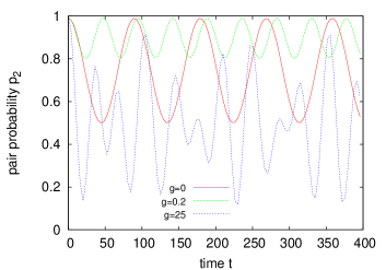
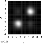
Figure 3: (color online) Top: Probability $p_{2}(t)$ of finding two atoms in the same well for $g=0,0.2,25$. Bottom: Snapshots of two-body correlation function $\rho_{2}(x_{1},x_{2})$ at equilibrium points, $\delta(t_{*})=0$, for $g=0$ ($t_{*}=44$), $g=0.2$ ($t_{*}=128$), and $g=25$ ($t_{*}=53$) – from left to right.

In order to unveil the physical content behind the tunneling dynamics, let us now investigate the two-body correlations. Noninteracting bosons simply tunnel independently, which is reflected in the two-body density $\rho_{2}(x_{1},x_{2})$. As a consequence, if both atoms start out in one well, then in the equilibrium point of the oscillation it will be as likely to find both atoms in the same well as in opposite ones. This is illustrated in Fig. 3, which exposes snapshots $\rho_{2}(x_{1},x_{2};t_{*})$ at the equilibrium points (where $\delta(t_{*})\stackrel{{\scriptstyle!}}{{=}}0$) and visualizes the temporal evolution of the pair (or same-site) probability

$$p_{2}(t) = \langle\Theta(x_{1})\Theta(x_{2})+\Theta(-x_{1})\Theta(-x_{2})\rangle_{t}$$

$$= \int_{\{x_{1}\cdot x_{2}\geq 0\}}\negthickspace\rho_{2}(x_{1},x_{2};t)dx_{1}dx_{2}.$$

As we introduce small correlations, the pair probability does not drop to $0.5$ anymore – at $g=0.2$ it notably oscillates about a value near 100%. This signifies that both atoms can essentially be found in the same well in the course of tunneling, which is apparent from the equilibrium-point image of $\rho_{2}$. In plain words, they tunnel as pairs. At this point, it is instructive to revisit the eigenstate analysis above: While the $g=0$ eigenstates $\Psi_{1,2}$ are delocalized, at intermediate $g=0.2$ they have basically evolved into superpositions $|N_{\mathrm{L}}=2,N_{\mathrm{R}}=0\rangle\pm|0,2\rangle$ of pair states localized in each well. In this light, the dynamics solely consists in shuffling the population back and forth between these two pair states.

Figure 3 in hindsight also casts a light on the fast (small-amplitude) modulations of $p_{\mathrm{R}}$ encountered in Fig. 1(a), namely by linking them to temporary reductions of the pair number $p_{2}$. Thus it is fair to interpret them as attempted one-body tunneling. Along the lines of the spectral analysis above, this relates to the contribution from the ground state, in which the two atoms reside in opposite wells and which does not join a doublet. Since $\Theta(x_{1})\Theta(x_{2})+\Theta(-x_{1})\Theta(-x_{2})$ is parity symmetric, only equal-parity matrix elements contribute to $p_{2}$, which yields $p_{2}(t)\approx 1-2p^{(02)}\sin^{2}\left(\omega_{02}t/2\right)$.

It is clear that, as before, the time evolution becomes more involved as the interaction energy is raised to the fermionization limit (cf. $g=25$). The two-body correlation pattern is fully fragmented not only when the pair is captured in one well (corresponding, e.g., to the upper right corner $x_{1},x_{2}\geq 0$), but also when passing through the equilibrium point $t=53$. These contributions from higher-band excited states also reflect in the evolution of $p_{2}(t)$, which is determined by the two modes $\omega_{\pm}=\Delta^{(0)}\pm\Delta^{(1)}$. Over time, $p_{2}$ passes through just about any value from $1$ (pair) to almost zero (complete isolation). In analogy to free fermions, it is again tempting to understand this involved pattern as two fermions tunneling independently with different frequencies.

IV.4 Many-body effects

Although having focused on the case of $N=2$ atoms so far, the question of higher atom numbers is interesting from two perspectives. For one thing, at stronger interactions many results become explicitly $N$-dependent, including distinctions between even/odd atom numbers zoellner06a ; zoellner07a . On the other hand, in a setup consisting of a whole array of 1D traps like in paredes04 ; kinoshita04 ; kinoshita06 , number fluctuations may automatically admix states with $N>2$.

IV.4.1 Complete imbalance

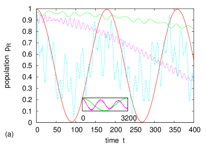
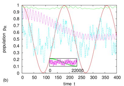
Figure 4: (color online) Time evolution $p_{\mathrm{R}}(t)$ of (a) $N=3$, (b) $N=4$ atoms initially in one well. Shown are the coupling strengths $g=0$ (—), $g=0.2$ (- - -), $g=4.7$ (${\color[rgb]{1,0,1}\cdots}$), and $g=25$ (${\color[rgb]{0,1,1}\boldsymbol{-\cdot-}}$). Insets: Long-time behavior for $g=0.2$ (the longer period) and $g=4.7$. (Observe the different time scales in both insets.)

For $N\geq 3$, the weak-interaction behavior does not differ conceptually. In fact, Eq. (3) carries over,

$$\delta(t)=\sum_{m<n}\delta^{(mn)}\cos(\omega_{mn}t),$$

but with the sum now running over $0\leq m<n\leq N$. Strictly speaking, the dynamics is thus no longer determined by two but rather in principle $N(N+1)/2$ modes $(mn)$ – although about half of these fail to contribute by symmetry. Nonetheless, the basic pattern can be understood from the two-atom case, as will become clear in a moment.

For $g=0$, assume an ideal initial state with all atoms in the right-localized orbital $\phi_{\mathrm{R}}=\frac{1}{\sqrt{2}}\left(\phi_{0}+\phi_{1}\right)$ of the lowest band. The weight coefficients $c_{N}(N_{0})=\langle N_{0},N-N_{0}|\Psi(0)\rangle$ with respect to the eigenstates $|N_{0},N_{1}\rangle$ have a binomial distribution

$$\left|c_{N}(N_{0})\right|^{2}=\frac{1}{2!^{N}}\binom{N}{N_{0}}\stackrel{{\scriptstyle N\to\infty}}{{\sim}}\delta_{\Delta N_{0}}(N_{0}-\bar{N}_{0})$$

which for larger $N$ asymptotically equals a Gaussian, with a sharp peak ($\Delta N_{0}=\sqrt{N}/2$) near $\bar{N_{0}}=N/2$. In this light, only these few states should contribute. Again, the equidistance of the levels guarantees a simple imbalance oscillation with $\Delta^{(0)}$. For interaction energies small compared to $\Delta^{(0)}$, the Rabi oscillations will again be modulated by beats, similar to the case $N=2$.

As we move to larger values $g\sim 0.2$, the higher-lying of the $N+1$ levels have again merged into doublets zoellner07a . In particular, the highest eigenstate pair was conjectured to be roughly of the form $|N_{\mathrm{L}}=N,N_{\mathrm{R}}=0\rangle\pm|0,N\rangle$ (in the limit $h\to\infty$). The idealized state distribution should be peaked at just these two vectors, whose energy splitting in the bare two-mode model has been estimated as $\omega\sim 2NU/(N-1)!\times(2\Delta^{(0)}/U)^{N}$ salgueiro06 , where $U$ denotes the on-site interaction energy. Thus the tunnel period is expected to grow exponentially as $N\to\infty$, a trend which may be roughly extrapolated from Fig. 4 (insets). Ultimately, this should connect to the condensate dynamics valid for $N\gg 1$ milburn97 ; tonel05 ; salgueiro06 ; creffield07 , when tunneling becomes inaccessible for all intents and purposes. Of course, realistically, neighboring states will also be excited, which makes the time evolution richer. However, the separation of time scales leads to the characteristic interplay of fast, small-amplitude oscillations (related to attempted single-particle tunneling) and a much slower tunnel motion, as observed in Fig. 4.

Things become more intricate if we leave the two-mode regime, cf. $g=4.7$. As has been demonstrated in zoellner07a , (anti-)crossings with higher-lying states (which connect to higher-band states at $g=0$) occur for $N\geq 3$. Given our experience of the two-atom case, one might again expect a simplified behavior as we approach the fermionization limit. However, we will argue below that this has to be taken with a grain of salt because an initial state with $N$ hard-core bosons in one well is highly excited. In the spirit of the Bose-Fermi map, an idealized state with $N$ fermions prepared in one well will have contributions from all excitations $|1_{a_{0}}^{(0)};1_{a_{1}}^{(1)};\dots;1_{a_{N-1}}^{(N-1)}\rangle_{\!-}$ ($a_{\beta}=0,1$ $\forall\beta$) in the $N$ lowest bands, which is proven by induction on $N=2$. In view of (4), many more frequencies are expected to be present: Besides the individual tunnel splittings $\Delta^{(\beta)}$ for each band, these should in principle be all four combinations $\Delta^{(0)}\pm\Delta^{(1)}\pm\Delta^{(2)}$ for $N=3$, and $4\times 4$ combinations $\{\Delta^{(l)}\pm\Delta^{(m)}\pm\Delta^{(n)}\mid 0\leq l<m<n\leq N\}$ for $N=4$ etc, taking into account parity-selection rules. However, in the fermionization limit with the idealized initial state above, things simplify even further. Since $\hat{N}_{\mathrm{R}}\equiv\sum_{\beta}a_{\mathrm{R}}^{(\beta)\dagger}a_{\mathrm{R}}^{(\beta)}$ —the Fock-space representation of $\Theta(x)$ in the context of Eq. (3)— is a one-particle operator, an eigenstate $|\boldsymbol{n}\rangle_{\!-}$ is coupled only to “singly excited” states of the type $|\boldsymbol{n}^{\prime}\rangle_{\!-}=a_{\mathrm{1}}^{(\beta)\dagger}a_{0}^{(\beta)}|\boldsymbol{n}\rangle_{\!-}$ (for some $\beta$), with an excitation frequency $\omega_{\boldsymbol{n},\boldsymbol{n}^{\prime}}=\Delta^{(\beta)}$. This yields an imbalance of

$$\delta(t)=\frac{1}{N}\sum_{\beta=0}^{N-1}\cos\Delta^{(\beta)}t\qquad(g\to\infty).$$

This simple formula should be contrasted with the surprising complexity of the fermionization dynamics already for atom numbers as small as $N=3,4$. This is illustrated in Fig. 4, where $p_{\mathrm{R}}(t)=[(\delta(t)+1]/2$ is plotted (cf. $g=25$). To be sure, for finite $g$ and using a realistic loading scheme, a few more modes contribute, thus naturally rendering the dynamics more irregular. But even the inocuous formula above can account for the seemingly erratic patterns in Fig. 4: The key to see this is to consider the distribution of frequencies $\{\Delta^{(\beta)}\}$. In the unrealistic limit that $\Delta^{(\beta)}\approx\Delta^{(0)}$ $\forall\beta$, the imbalance would be a neat Rabi oscillation for any $N$, $\delta(t)\approx\cos\Delta^{(0)}t$. However, a realistic barrier likely has a Gaussian-type shape and a finite height; hence the splittings of higher bands tend to grow monotonically. As a consequence, only the lower-band frequencies $\Delta^{(\beta)}$ will contribute to the tunneling, whereas the higher-band splittings make for much faster modulations, which average out on a larger time scale. The gist is that for $N\gg 1$, those few lowest-band modes only have a weight of $O(1/N)$, so in a realistic scenario one expects quasi-equilibration around $p_{\mathrm{R}}=1/2$.

IV.4.2 Partial imbalance

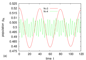
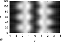
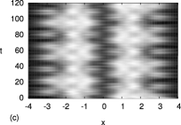
Figure 5: (color online) Partial-imbalance effects in the fermionization limit ($g=25$). (a) Small-imbalance oscillations (Scenario 1.) for $N=3,4$ atoms. Plotted is the population of the right-hand well, $p_{\mathrm{R}}(t)$. Bottom: Density evolution $\rho(x;t)$ for $N-1=2$ (b) and $N-1=3$ atoms (c) initially in the right-hand well if exactly one atom is present on the left (Scenario 2.).

While we have so far assumed that all atoms are prepared in one well, it is natural to ask what the effect of incomplete imbalances $p_{\mathrm{R}}(0)<1$ would be. For simplicity, we will focus on the fermionization limit (here $g=25$). Two scenarios are conceivable, in principle:

1. Small imbalances $p_{\mathrm{R}}\approx 1/2$, i.e., small perturbations of the ground state;

2. Preparing, say, $N-1$ atoms in one well and one in the other.

Option (1.) is plotted in Fig. 5(a) for $N=3,4$. We clearly observe Josephson-type oscillations in each case, but with markedly different time scales. This may be understood from the spectral structure near fermionization zoellner07a : For even $N$, the fermionic ground state $|1_{0}^{(0)},1_{1}^{(0)},\dots,1_{0}^{(N/2-1)},1_{1}^{(N/2-1)}\rangle_{\!-}$ has all bands filled, so that the lowest excitation is created by moving one atom from band $\beta=N/2-1$ to $\beta=N/2$. Thus the “Josephson” frequency $\omega_{01}=\epsilon_{0}^{(N/2)}-\epsilon_{1}^{(N/2-1)}$ is a large inter-band gap, which for $N=4$ gives a period of $T_{01}\approx 4$. For odd $N$, by contrast, the mechanism is a different one: Here the ground state leaves the highest band only singly occupied, so that the lowest excitation frequency is the small intra-band splitting $\omega_{01}=\Delta^{(N-1)/2}$. In Fig. 5(a) ($N=3$), this may be identified as the rather long period $T_{01}\approx 40$.

Scenario (2.), paraphrased in the case $N=3$, is the question of the fate of an atom pair if the target site (the left well) is already occupied by an atom. The striking answer, as evidenced in Fig. 5(b), is that the process can be viewed as single-atom tunneling on the background of the symmetric two-atom ground state. The tunneling frequency in the fermionization limit is $\Delta^{(1)}\approx 2\pi/40$, which has the intuitive interpretation of a fermion which—lifted to the band $\beta=1$—tunnels independently of the two lowest-band fermions. From that point of view, it should come as no surprise that adding another particle destroys that simple picture. In fact, Fig. 5(c) reveals that if we start with $N-1=3$ atoms on the right, then the tunneling oscillations appear erratic at first glance, and a configuration with three atoms per site becomes an elusive event (see, e.g., $t\approx 22,44$ or $72$). In the fermionic picture, this can be roughly understood as superimposed tunneling of one atom in the first excited band ($\Delta^{(1)}$) and another in the second band ($\Delta^{(2)}\approx 2\pi/15$), while the remaining zeroth-band fermions remain inactive.

V Asymmetric double well

We have so far used the tilt $d$ of the double well merely as a tool to load the atoms into one well. The question naturally arises whether the actual tunnel oscillations can be studied in asymmetric wells so as to manipulate the nature of the tunneling. Specifically, we consider a setup similar to Sec. IV: Two atoms are prepared in the right well (i.e., in ground state $\Psi_{0}^{(d_{0})}$with a large initial asymmetry $d_{0}$). Subsequently, the asymmetry is ramped down to a final value $d\neq 0$, thus triggering the tunnel dynamics.

V.1 Tuning tunneling resonances

In symmetric wells, pair tunneling is always resonant in the sense that an initial state with all atoms on one site is equal in energy to one with all atoms in the opposite well dounasfrazer07b ; foelling07 . Conversely, single-atom tunneling should only be likely so long as the repulsive interaction does not shift the pair state’s energy off resonance with a target state of only a single atom on the left. This squares with our finding that the pair probability $p_{2}$ (Fig. 3) drops to 50% in the equilibrium points for $g=0$, while in the correlated case ($g=0.2$) it does not vary considerably from unity. To condense this insight into a single quantity, let us define

$$\bar{p}_{1}=\max_{t>0}\{1-p_{2}(t)\}$$

as the (maximum) single-atom probability, relating to the event of finding the atoms in different wells.

Figure 6 shows how $\bar{p}_{1}$ changes when the final asymmetry $d$ between the wells is varied. For $g=0$, $\bar{p}_{1}(d)$ has a plateau for $d\leq 0.011$. This relates to the transition from coexistence of single-atom and pair tunneling (at $d=0$) to the point where the right-hand well is lowered such in energy that the initial pair state energetically matches a state with exactly one atom on the left. From the perspective of the two-body density in Fig. 3, the final state at $d=0.011$ corresponds to the equilibrium-point snapshot for $d=0$. For larger values of $d$, the energy difference between both wells is too large to transfer a substantial fraction of the population to the other well.

By contrast, at $g=0.2$ the repulsion is sufficiently strong to drive the single-atom tunneling off resonance at $d=0$ (Fig. 6). Lowering the right well so as to compensate for the interaction-energy shift leads to a dramatic increase of the tunnel amplitude near $d=0.038$. The value of $\bar{p}_{1}\approx 1$ confirms that this is pure single-atom tunneling: After half a tunnel period, both atoms are found precisely in opposite wells, until they return to the pair state on the right site.

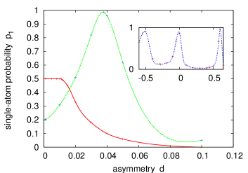
Figure 6: (color online) Maximum single-atom probability $\bar{p}_{1}$ as a function of the tilt parameter $d$. Solid line: uncorrelated tunneling, $g=0$; dashed line: correlated tunneling, $g=0.2$. Inset: Near the fermionization limit, $g=25$. Note that the resonances are not symmetric in $d$ owing to the unsymmetric initial state $\Psi(0)$.

Despite the more convolved dynamics that emerges as we go higher interactions, the one-atom tunnel resonance persists. However, in the fermionization limit $g\to\infty$, yet another resonance emerges at $d=0$ already (Fig. 6). As in the uncorrelated case, this signifies coincident single-atom and pair tunneling. This resonance, however, is much more sensitive to symmetry breaking, which is intelligible from the picture of two fermions hopping simultaneously in different bands $\beta=0,1$. Skewing the double well ($d>0$) thus attenuates both one- and two-atom tunneling until another, pure single-atom resonance is hit at $d=0.58$. Conversely, energetically lifting the right-hand well ($d\approx-0.5$) makes tunneling to excited target states accessible.

V.2 Spectral analysis

To better understand the dependence of the tunnel dynamics on the tilt $d$, let us consider the two-body spectrum $\{E_{m}(d)\}$ at fixed coupling $g$. Since both the noninteracting and the fermionization limit can be deferred from the single-particle spectrum, we will first stop to review the tilted double well.

V.2.1 One-body spectrum

Figure 7: Single-particle spectrum $\{\epsilon_{a}(d)\}$ of a double well as a function of the asymmetry $d$.

Figure 7 displays the spectrum $\{\epsilon_{a}(d)\}$ of the double well $U(x)=\frac{1}{2}x^{2}+h\delta_{w}(x)-d\cdot x$ for variable asymmetries $d$. For simplicity, let us resort to a simple model and expand the one-body Hamiltonian $h(p,x)=\frac{1}{2}p^{2}+U(x)$ in terms of two modes $\phi_{\alpha=\mathrm{L(R)}}$ localized on the left (right) site (tacitly assuming a fixed band $\beta$). We denote by

• $\langle\phi_{\alpha}|h|\phi_{\alpha}\rangle=\bar{\epsilon}\pm\varsigma/2$ the energies pertaining to isolated wells, where the left site has an energy offset $\varsigma$

• $\left|\langle\phi_{\mathrm{L}}|h|\phi_{\mathrm{R}}\rangle\right|=\Delta/2$ the tunnel coupling.

Then a straightforward diagonalization yields

$$\phi_{a,\varsigma} \propto \Delta\cdot\phi_{\mathrm{L}}+\left[\varsigma\pm\Delta(\varsigma)\right]\phi_{\mathrm{R}}\qquad(a=0,1)$$

$$\epsilon_{a,\varsigma} = \bar{\epsilon}\mp{\scriptstyle\frac{1}{2}}\Delta(\varsigma)$$

where $\Delta(\varsigma)\equiv\sqrt{\Delta^{2}+\varsigma^{2}}$ is the energy gap in the presence of the tilt. In the symmetric case, the states are simply given by the (anti-)symmetric orbitals $\phi_{a,\varsigma=0}\propto\phi_{\mathrm{L}}\pm\phi_{\mathrm{R}}$, with the usual tunnel splitting $\Delta(0)\equiv\Delta$. As we switch on a tilt $\varsigma>0$, parity is broken and the once delocalized states break up into one decentered on the left ($\phi_{1}$) and one on the right ($\phi_{0}$) as $\varsigma\gg\Delta$. This goes along with a level repulsion of $\epsilon_{0/1,\varsigma}$ about $\varsigma=0$, where the $\phi_{1}$ state pinpointed on the left site is energetically lifted, and vice versa. As the states decouple for $\varsigma\gg\Delta$, the energy approaches that of the isolated subsystem $\epsilon_{a,\varsigma}\sim\bar{\epsilon}\mp\varsigma/2$.

The above picture holds for each band $\beta$ individually, provided their levels are well separated. In fact, Fig. 7 confirms that scenario for tilts small compared to the interband gap, $\varsigma\ll\bar{\epsilon}^{(\beta+1)}-\bar{\epsilon}^{(\beta)}\sim 2$. For strong enough asymmetries $d$, though, states emerging from different bands mix, and new avoided crossings are observed in the plot.

V.2.2 Two-body spectrum

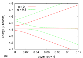
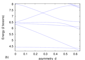
Figure 8: (color online) Two-body spectrum $\{E_{m}(d)\}$ in a tilted double well. (a) $g=0,\,0.2$ (b) $g=25$.

Noninteracting limit:

In the uncorrelated system, $g=0$, the many-body spectrum $\{E_{\boldsymbol{n}}=\sum_{a}n_{a}\epsilon_{a}\}$ is obtained from the number states $|\boldsymbol{n}\rangle$ of the single-particle eigenstates $\phi_{a}$. The energy shift of the levels $E_{\boldsymbol{n}}(d)$ with respect to $d=0$ thus depends on the balance between contributions from symmetric orbitals $\phi_{0}^{(\beta)}$ and antisymmetric ones. Specifically, the $d=0$ ground state exhibited in Fig. 8(a) is a coherently symmetric state $|20\rangle=[\phi_{0}^{(0)}]^{\otimes 2}$. Consistently, for perturbations $d>0$ it localizes on the right, with its level shifting downward – in stark contrast to the second excitation $|02\rangle=[\phi_{1}^{(0)}]^{\otimes 2}$. In between, $|11\rangle$ is a compromise between these two borderline cases in that both partial energy shifts cancel out, leaving a delocalized state. This gives us a new perspective on the tunneling dynamics reflected in Fig. 6. Imagine we start with all atoms prepared in the right well, viz., the ground state $\Psi_{0}^{(d\to\infty)}$, and then ramp down $d(t)\to 0$ so as to trigger the tunneling. If we follow the ground-state level nonadiabatically, then at $d=0$ it finds three closely packed levels $E_{m}(0)$ it can couple to – in the sense that $\left|\langle\Psi_{m}|\Psi(0)\rangle\right|\neq 0$, so that a nontrivial dynamics becomes possible. In fact, at $d=0$, these correspond to Rabi oscillations. If we were to choose a final asymmetry $d\stackrel{{\scriptstyle<}}{{\sim}}0.01$ (in the notation above, $\varsigma^{(0)}<\Delta^{(0)}$), roughly the same level would be available, confirming the plateau encountered in Fig. 6. However, for final values $d>0.01$, the levels decouple, and no longer are there any target states at disposal for tunneling.

Medium interactions:

These elementary thoughts also help us explore the nontrivial dynamics for intermediate couplings, as shown for $g=0.2$ in Fig. 8(a). The $d=0$ ground state, in the limit $\Delta^{(0)}\to 0$, has the Mott-insulator form $|1_{\mathrm{L}}1_{\mathrm{R}}\rangle$ and should be insensitive to symmetry breaking $d>0$. By contrast, the quasi-degenerate excited pair $|2_{\mathrm{L}}0_{\mathrm{R}}\rangle\pm|0_{\mathrm{L}}2_{\mathrm{R}}\rangle$ only requires a minute perturbation to break up into two localized states. It is plain to see that, at $d\approx 0.04$, the lower excited curve anti-crosses the ground state, and the two states are virtually swapped. Resorting again to a simple two-mode model, the (avoided) crossing occurs for tilts $\varsigma=U$ matching the on-site repulsion energy.

The bearing this has on the tunnel dynamics is evident: Apart from the self-trapping scenario at $d=0$, there is a fairly broad tunnel resonance at $d\approx 0.04$, where the fully imbalanced initial state $\Psi(0)$ couples to that with one atom on each site, $|1_{\mathrm{L}}1_{\mathrm{R}}\rangle$. This is but the one-body resonance encountered in Fig. 6. To come by a crude estimate for the critical value $d_{c}$, assume that the energy of initial and final states match, $\langle H_{d_{c}}\rangle_{\mathrm{i}}=\langle H_{d_{c}}\rangle_{\mathrm{f}}$. Modeling the initial pair state by the ground state $\Psi_{0}^{(d_{0})}$ (at the initial $d_{0}>0$), and the final state with a single atom on the left by $\Psi_{0}^{(0)}$, yields the estimate

$$d_{c}=d_{0}-\left(E_{0}^{(0)}-E_{0}^{(d_{0})}\right)/N\left\langle x\right\rangle^{(d_{0})}$$

in terms of the ground-state energies at the initial $d_{0}>0$ and $d=0$, respectively, and the elongation $\left\langle x\right\rangle$ at time $t=0$.

Fermionization limit:

Figure 8(b) shows the spectrum near fermionization, $g=25$. The $d=0$ ground state turns out to be widely robust against perturbations, which can be understood from the fact that its fermionic counterpart $|1_{\mathrm{0}}^{(0)}1_{1}^{(0)}\rangle_{\!-}$ has balanced populations of right- and left-localizing orbitals. The only way to obtain a right-localized ground state is to lower one well enough for it to hit a localized state from the upper band. This is what happens at $d\approx 0.6$, where the tilt energy $\varsigma^{(1)}/2=\bar{\epsilon}^{(1)}-\bar{\epsilon}^{(0)}$ compensates the inter-band gap. That crossing marks just the one-body resonance seen in Fig. 6 at $d\approx 0.6$. In the fermionic picture invoked above, it may be thought of as one excited fermion tunneling to the lowest level on the left.

If we follow the localized state nonadiabatically, then at $d=0$ we recover the mixed single-atom/pair resonance laid bare in Fig. 6. Further ramping up the right well to $d\approx-0.3$ (where the spectrum is mirrored at $d=0$), we see yet another crossing. A closer look reveals that the partner state is entirely localized on the left, so that one might hope for a pair resonance. However, as both states are localized in disjoint regions, they are not coupled by the perturbation ($-d\cdot x$), and in practice no tunnel resonance is observed. It may be illuminating to look at this from the fermionic perspective. For $d\approx-0.3$, the initial state on the right is $\Psi(0)\approx|1_{1}^{(0)}{;1}_{1}^{(1)}\rangle_{\!-}$, while the partner state emanating from $E(0)\approx 8$ in turn is given by $|1_{0}^{(0)}{;1}_{0}^{(2)}\rangle_{\!-}$. In this light, the tunneling “resonance” in question refers to the following situation: Two fermions simultaneously hop from the zeroth (first excited) level on the right down to the zeroth level (up into the second level) of the energetically lower left site. While both processes individually are off resonance, the total energy is conserved. This reflects in the one-body spectrum (Fig. 7), where no avoided crossing is to be observed at $d\approx-0.3$ – rather, there is an accidental crossing of the sums $E_{\boldsymbol{n}}=\sum_{a}n_{a}\epsilon_{a}$. However, at $d\approx-0.6$, another avoided crossing emerges, which—in the fermion language—corresponds to multiple one-body resonances with the first and second excited level in the left well.

VI Conclusions and outlook

We have analyzed the crossover from uncorrelated to fermionized tunneling of few 1D bosons in a double well. The pathway leads via strongly delayed pair tunneling for medium interactions—associated with doublet formation in the few-body spectrum—to fermionized tunneling, where the strongly correlated atoms tunnel back and forth with characteristic modulations. By analogy to free fermions, these may be understood as multi-band Rabi oscillations, which become more and more complex and quasi-equilibrate for large atom numbers. To uncover the physical mechanisms, it is essential to study two-body correlations. These reveal a strong suppression of single-atom tunneling for intermediate coupling, with a revival toward fermionization, where an involved interplay of pair and single-atom tunneling is observed.

Whereas for small interactions, higher atom numbers essentially only increase the tunnel period but do not change the scenario qualitatively, the multi-atom dynamics becomes much richer as fermionization is approached. Apart from the above case of a complete initial imbalance, this applies to situations where not all atoms are initially in one well. In particular, Josephson-type small-amplitude oscillations exhibit vastly different time scales for odd/even numbers. On the other hand, initially storing an extra atom in the target well suppresses the lowet-band tunneling and thus leads to a simplified dynamics.

Finally, studying the dynamics in asymmetric wells provides a valuable perspective on the tunnel mechanism in terms of one- and two-atom tunnel resonances. Depending on the energy difference between the sites, the tunnel amplitude can be largely enhanced or suppressed. For noninteracting bosons, this has been described by a plateau of the single-atom probability about the asymmetry parameter $d=0$. At medium interactions, in turn, single-particle tunneling becomes resonant only when the energy offset of one well compensates the interaction-energy shift at $d>0$. In the fermionization limit, another $d=0$ resonance emerges, accompanied by higher-level resonances at $d\neq 0$. Those features are explained in terms of avoided crossings in the spectrum as $d$ is varied. Such a deeper understanding of the tunneling may pave the way to an active control of strongly correlated systems, for instance by allowing to transport definite numbers of atoms from a reservoir to a target well.

- (1) L. Pitaevskii and S. Stringari, Bose-Einstein Condensation (Oxford University Press, Oxford, 2003).
- (2) F. Dalfovo, S. Giorgini, L. Pitaevskii, and S. Stringari, Rev. Mod. Phys. 71, 463 (1999).
- (3) C. J. Pethick and H. Smith, Bose-Einstein condensation in dilute gases (Cambridge University Press, Cambridge, 2001).
- (4) A. J. Leggett, Rev. Mod. Phys. 73, 307 (2001).
- (5) M. Albiez et al., Phys. Rev. Lett. 95, 010402 (2005).
- (6) G. J. Milburn, J. Corney, E. M. Wright, and D. F. Walls, Phys. Rev. A 55, 4318 (1997).
- (7) A. Smerzi, S. Fantoni, S. Giovanazzi, and S. R. Shenoy, Phys. Rev. Lett. 79, 4950 (1997).
- (8) T. Anker et al., Phys. Rev. Lett. 94, 020403 (2005).
- (9) J. Javanainen, Phys. Rev. Lett. 57, 3164 (1986).
- (10) K. Winkler et al., Nature 441, 853 (2006).
- (11) S. Fölling et al., Nature 448, 1029 (2007).
- (12) T. Köhler, K. Góral, and P. S. Julienne, Rev. Mod. Phys. 78, 1311 (2006).
- (13) M. Olshanii, Phys. Rev. Lett. 81, 938 (1998).
- (14) M. Girardeau, J. Math. Phys. 1, 516 (1960).
- (15) B. Paredes et al., Nature 429, 277 (2004).
- (16) T. Kinoshita, T. Wenger, and D. S. Weiss, Science 305, 1125 (2004).
- (17) T. Kinoshita, T. Wenger, and D. S. Weiss, Nature 440, 900 (2006).
- (18) M. D. Girardeau and E. M. Wright, Phys. Rev. Lett. 84, 5691 (2000).
- (19) K. K. Das, M. D. Girardeau, and E. M. Wright, Phys. Rev. Lett. 89, 170404 (2002).
- (20) T. Busch and G. Huyet, J. Phys. B 36, 2553 (2003).
- (21) A. Minguzzi and D. M. Gangardt, Phys. Rev. Lett. 94, 240404 (2005).
- (22) O. E. Alon and L. S. Cederbaum, Phys. Rev. Lett. 95, 140402 (2005).
- (23) F. Deuretzbacher, K. Bongs, K. Sengstock, and D. Pfannkuche, Phys. Rev. A 75, 013614 (2007).
- (24) S. Zöllner, H.-D. Meyer, and P. Schmelcher, Phys. Rev. A 74, 053612 (2006).
- (25) S. Zöllner, H.-D. Meyer, and P. Schmelcher, Phys. Rev. A 74, 063611 (2006).
- (26) S. Zöllner, H.-D. Meyer, and P. Schmelcher, Phys. Rev. A 75, 043608 (2007).
- (27) S. Zöllner, H.-D. Meyer, and P. Schmelcher, cond-mat/0709.3163 .
- (28) A. P. Tonel, J. Links, and A. Foerster, J. Phys. A 38, 1235 (2005).
- (29) A. N. Salgueiro et al., Eur. Phys. J. D 44, 537 (2007).
- (30) C. E. Creffield, Phys. Rev. A 75, 031607 (2007).
- (31) D. R. Dounas-Frazer and L. D. Carr, quant-ph/0610166 .
- (32) H.-D. Meyer, U. Manthe, and L. S. Cederbaum, Chem. Phys. Lett. 165, 73 (1990).
- (33) M. H. Beck, A. Jäckle, G. A. Worth, and H.-D. Meyer, Phys. Rep. 324, 1 (2000).
- (34) G. A. Worth, M. H. Beck, A. Jäckle, and H.-D. Meyer, The MCTDH Package, Version 8.2, (2000). H.-D. Meyer, Version 8.3 (2002). See http://www.pci.uni-heidelberg.de/tc/usr/mctdh/.
- (35) R. Kosloff and H. Tal-Ezer, Chem. Phys. Lett. 127, 223 (1986).
- (36) H.-D. Meyer and G. A. Worth, Theor. Chem. Acc. 109, 251 (2003).
- (37) H.-D. Meyer, F. L. Quéré, C. Léonard, and F. Gatti, Chem. Phys. 329, 179 (2006).
- (38) D. R. Dounas-Frazer, A. M. Hermundstad, and L. D. Carr, Phys. Rev. Lett. 99, 200402 (2007).