Measurement of the Total Charm Cross Section by Electron-Positron Annihilation at Energies Between 3.97-4.26 GeV

Abstract

Using the CLEO-c detector, we have measured the charm hadronic cross sections for $e^{+}e^{-}$ annihilations at a total of thirteen center-of-mass energies between 3.97 and 4.26 GeV. Observed cross sections for the production of $D\bar{D}$, $D^{*}\bar{D}$, $D^{*}\bar{D}^{*}$, $D_{s}\bar{D}_{s}$, $D_{s}^{*}\bar{D}_{s}$, and $D_{s}^{*}\bar{D}_{s}^{*}$, in addition to the total charm cross section are presented. Observed cross sections were radiatively corrected to obtain tree-level cross sections and R.

University of Minnesota Physics Professor Yuichi Kubota, Ph.D. and Professor Ronald Poling, Ph.D. 64

To my wife, my family, and my friends for all of their love, support and most importantly their patience.

Acknowledgement - [ak-nol-ij-muh nt] An expression of appreciation or gratitude. I have been so lucky during my time at the University of Minnesota: lucky to have received supportive advisors, lucky to have been part of an innovative, collaborative group, and damn lucky to have such a loving network of friends and family. I would like to express my appreciation and gratitude on these first pages of my dissertation.

• I would like to thank my advisors Yuichi Kubota and Ron Poling for their support over the years. Their continual patience, insight, and suggestions have no doubt helped me get to this point in my career. Their enthusiasm, curiosity and passion for physics and of tackling problems is truly inspirational. It was certainly a pleasure to have worked with and learn from such fine physicists.

• I would also like to thank the other University of Minnesota group members both past and present: Valery Frolov, Kaiyan Gao, Datao Gong, Selina Li, Alexander Scott, and Chris Stepaniak. Tim Klein, who was always willing to lend a hand, in addition to making the best mojito in town. Prof. Dan Cronin-Hennessy’s willingness and ability to add insight to perplexing and complicated questions and problems. Alex Smith, for alway having his door, or cubicle, open for questions and discussions. In particular, I would like to send thanks to Justin Hietala and Pete Zweber for their many discussions with me about my analysis and of physics in general. Additional thanks to Pete for, among these discussions, he was willing to be my chauffeur, tour guide, and social director while in Ithaca, New York.

• I would like to thank the many people that have supported me during this long process. I can only work so much, right?!? I would like to thank Jim and Kara Melichar, Tom O’Connor, Justin Holzman, Mark McCarthy, Brian Gulden, Maggie Edmiston, Steve Udycz, Joe Skinner, Jake Kern, Nathan Moore, Sarah and Paul Way, Andy Cady, Erik Beall, Paul Barsic, Pete Vassy, Christine Crane, Adrienne Zweber, Norm Lowrey, Curtis Jastremsky, Paras Naik, Mike Watkins, Laura Adams, and Lynde Klein. Special kudos to my softball team, Quit Yer Pitchin’, for a painful and slightly embarrassing, yet enjoyable few seasons. These people, and countless others, have made my graduate school days in Minnesota fulfilling and adventurous. As a result, I have many stories and memories to keep with me always.

• I would also like to send thanks for the overwhelming love and support of my family. My parents, John and Kathy Lang, have always taught me the value of hard work and persistence. I would also like to thank my grandmothers, Betty Walchli and Colletta Lang, my brother, Mike, sister-in-law, Brandy, and nephew, Michael, and my Aunt and Uncle Tricia and Tom Sweeney, as well as my adoring mother-in-law, Cheryl Clever (C.L.).

  I would also like to take a moment to thank those family members who had supported me throughout these many years, and who are now celebrating with me in spirit. Thank you to my grandfathers, William F. Walchli and Russell Lang and to my favorite little brother (in-law), Adam Clever.

• Finally, but most certainly not least, I would like to thank my wife, Sarah, for whom I am extremely thankful. Her love, friendship, patience, encouragement, and sense of humor, have given my life immense purpose, joy, and meaning. The finished work that is to follow would have no meaning or satisfaction without having her with me to share it. I love you Angle!

Chapter Introduction

This dissertation is devoted to the study of charm-meson production in $e^{+}e^{-}$ annihilations at thirteen center-of-mass energies between 3.97 GeV and 4.26 GeV. Specifically, we have used the CLEO-c detector to measure exclusive cross sections for several final states and the inclusive cross sections for the production of the charmed mesons $D^{0}$, $D^{+}$ and $D_{s}$. To provide the background for this research I first review some of the foundations of elementary particle physics, including the Standard Model of quarks and leptons.

During the past century, our understanding of nature and structure of matter has been dramatically transformed, beginning with the discovery that atoms are divisible structures composed of subatomic particles. With this discovery and others the modern picture began to form of atoms consisting of a positively charged nucleus surrounded by negatively charged electrons.

Elementary particle physics is the study of the fundamental constituents of matter and their interactions. It began with the discoveries of the electron (Thomson), atomic nucleus (Rutherford) and the neutron (Chadwick), developing slowly at the same time that the theoretical foundations of quantum mechanics were being laid. Meanwhile, investigation of cosmic rays and the development of accelerator-based experiments in the 1940’s, 1950’s, and the 1960’s led to the discovery of many more particles, particles that do not exist in ordinary matter. With the seemingly endless additions of new particles, the sentiment grew that there must be another level of substructure to explain this particle “zoo”. This sentiment ultimately led to the invention, by Gell-Mann and Zweig [1], of a model that describes most observed particles as being composed of the more fundamental particle known as the quark.

1 The Standard Model

The modern framework which describes the fundamental particles and interactions is called the Standard Model. The Standard Model incorporates the quarks and the leptons (the electron and its relatives) into a successful framework that has proven to be very rugged and reliable over the years. The quarks and leptons are said to be fundamental because they are structureless: they are point-like and indivisible. Even though they are structureless, however, they still possess intrinsic properties such as spin, charge, color, etc. All particles but one can be arranged into three groups: quarks, leptons, and force carriers or mediators. The remaining particle, the Higgs boson, has a special job in the model. The Higgs is the last remaining particle of the Standard Model yet to be discovered. It plays the key role in explaining the mass of the other particles, specifically the large mass difference between the photon, the vector bosons and the quarks.

The leptons come in six types which are listed in Table 1 along with their corresponding masses and charges. The lightest charged lepton is the familiar electron. The muon ($\mu$) and tau ($\tau$) have the same general properties as the electron, but they have larger masses. These heavier versions are unstable and therefore not found in ordinary matter. Each charged lepton is accompanied by a weakly interacting electrically neutral neutrino: $\nu_{e}$, $\nu_{\mu}$, and $\nu_{\tau}$. Together each lepton and its accompanying neutrino form a family, sometimes referred to as a generation. All leptons have intrinsic angular momentum, or spin, of $\frac{1}{2}\hbar$ and are therefore fermions.

Table 1: The six types of leptons in the Standard Model. The masses are taken from Ref. [2]. The electric charges are given in units of $|e|$, where $e$ is the charge of an electron ($|e|=1.602\times 10^{-19}$ Coulombs). The neutrino’s masses are given at $95\%$ confidence level.

Family	Name	Electric	Mass
		Change $\frac{Q}{|e|}$
I	$e$	$-1$	511 keV
	$\nu_{e}$	$0$	$<$3 eV
II	$\mu$	$-1$	106 MeV
	$\nu_{\mu}$	$0$	$<$0.19 MeV
III	$\tau$	$-1$	1.78 GeV
	$\nu_{\tau}$	$0$	$<$18.2 MeV

Similarly, the quarks also come in six types, which can also be split into three generations. The first generation of quarks consists of the up ($u$) and down ($d$). Together with the electron the first generation of quarks make up all the ordinary matter around us. The second generation (strange ($s$) and charm ($c$) quarks) and the third generation (bottom ($b$) and top ($t$) quarks) make-up the rest of the known quarks. Since they have intrinsic angular momentum of $\frac{1}{2}\hbar$, all quarks are fermions. Some properties of the quarks are shown in Table 2. Quarks are never individually observed but rather are seen only in combinations called hadrons. There are two types of hadrons: mesons, which are bound states of a quark and an anti-quark, and baryons, which are bound states of three quarks or anti-quarks.

Table 2: The six types of quarks in the Standard Model. The masses are taken from Ref. [2]. The electric charges are given in units of $|e|$, where $e$ is the charge of an electron ($|e|=1.602\times 10^{-19}$ Coulombs). The quark masses are approximate since the complicated strong interactions that take place inside the hadrons make it difficult to define and measure the individual quark masses. However, because of its short lifetime, the top quark does not have time to bind into hadrons, and therefore it has the smallest fractional uncertainty on its mass.

Family	Name	Electric	Mass
		Change $\frac{Q}{|e|}$
I	$u$	$+\frac{2}{3}$	1-4 MeV
	$d$	$-\frac{1}{3}$	4-8 MeV
II	$c$	$+\frac{2}{3}$	1.15-1.35 GeV
	$s$	$-\frac{1}{3}$	80-130 MeV
III	$t$	$+\frac{2}{3}$	174 GeV
	$b$	$-\frac{1}{3}$	4.1-4.4 GeV

The interactions among these fundamental particles are the four forces: strong, weak, electromagnetic, and Gravitational. Of these, Gravity is by far the weakest, plays no role in the interactions described in this dissertation, and is not part of the Standard Model. In the Standard Model the three remaining forces are represented as an exchange of gauge bosons between interacting particles. All gauge bosons have integer spin, and some of their properties are shown in Table 3. Of the fundamental fermions, only the quarks interact through the action of all three forces. The charged leptons experience only the weak and electromagnetic forces, and the neutrinos interact only via the weak force.

Table 3: The gauge bosons in the Standard Model. The masses are taken from Ref. [2]. The electric charges are giving in units of $|e|$, where $e$ is the charge of an electron ($|e|=1.602\times 10^{-19}$ Coulombs).

Force	Name	Electric	Mass
		Change $\frac{Q}{|e|}$
strong	gluons $g$	$0$	0
weak	W-Bosons $W^{\pm}$	$\pm 1$	80.4 GeV
	Z-Boson $Z^{0}$	$0$	91.2 GeV
electromagnetic	Photon $\gamma$	$0$	0

The electromagnetic force is responsible for the binding of electrons to the nucleus inside the atom. The mediator of this force, the photon, couples to electrically charged particles. The quantum theory describing the electromagnetic interaction is called Quantum Electrodynamics (QED) and has been extensively tested. QED is the most accurate physical theory constructed.

The weak interaction was first discovered in nuclear decays. All fundamental fermions, including the neutrinos, participate in the weak interaction. The mediators of the weak force are the vector bosons, the $W^{\pm}$ and the $Z$, which are massive, explaining its very short range, since the range is proportional to $1/M$. Interactions involving the charged $W$-bosons involve changes the flavor of the particles involved. These changes can lead to spontaneous decays of the type $\mu^{-}\rightarrow{e^{-}}\bar{\nu}_{e}\nu_{\mu}$. Since the decay involves the charged $W$-boson, these types of interactions are known as “charged current” interactions.

The strong force involves the exchange of gluons between particles possessing “color charge” [3], which is analogous to the electric charge. The only fundamental particles possessing color charge are the quarks and gluons. Therefore, the leptons do not participate in strong interactions. Each quark carries one of the three colors, usually denoted red ($r$), green ($g$), and blue ($b$), while the anti-quarks carry anti-color: $\bar{r}$, $\bar{g}$, and $\bar{b}$. The quantum theory which describes the strong force is known as quantum chromodynamics (QCD).

One interesting aspect of QCD is color confinement, the feature that no free quarks exist in nature. Rather, quarks must bind into the composite particles known as hadrons, are color-neutral. Therefore the anti-quark of the meson will have the anti-color of its quark partner, while for a baryon each quark will possess a different color. The origin of the confinement is related to the fact that gluons themselves carry color and therefore interact with each other. As two quarks are pulled apart, the gluon-gluon interactions form a narrow tube resulting in a constant force. As the separation of the two quarks increases, so does the energy, until at some distance it becomes energetically favorable to “pop” out quarks from the vacuum to “dress” the quarks into hadrons. Confinement is not a feature of QED since the photon is electrically neutral. That is, as two charged particles get pulled apart, the force between them decreases allowing atoms to ionize.

Another interesting aspect of QCD is asymptotic freedom [4]. As the momentum transferred in an interaction increases, the strength, or coupling, in the interaction decreases. Therefore, in these types of interactions, perturbative methods can be applied to the calculations, as they are in QED. However, because the strength of the interaction increases at lower momenta, QCD calculations are very difficult in most cases.

Since this thesis is devoted to the production of charm mesons, a dedicated review of charm follows in the next section.

2 Charm

The quark model, when it was introduced by Gell-Mann and independently by Zweig in 1964, explained all hadrons matter as being combinations of three kinds of quarks: up ($u$), down ($d$), and strange ($s$). Initially, there was no experimental reason for any additional quarks, but Bjorken and Glashow [5], as a way of making nature more symmetrical at a time when there were three known quarks and four known leptons, predicted the existence of the yet-to-be discovered charm ($c$) quark. The Glashow-Iliopoulos-Maiani (GIM) mechanism [6, 7] made the case for charm more compelling, explaining the experimentally unobserved strangeness-changing neutral currents (SCNC) in the theory by adding charm in a particular way to the weak hadronic current which would otherwise be expected.

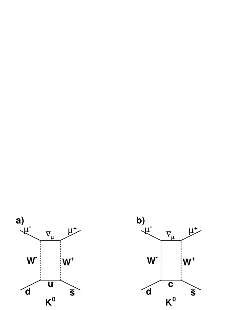
Figure 1: The decay of $K^{0}\rightarrow\mu^{+}\mu^{-}$ and the GIM mechanism. The only difference between a) and b) is the virtual quark, that is the $u$ quark is replaced by the $c$ when going from a) to b). The decay vanishes with the addition of the charm quark, thus eliminating strangeness-changing neutral currents as demanded by the data.

In 1963, Cabibbo had noticed that the decay rates of strange particles differed from those of non-strange particles [8]. For example, the decay rate for $K^{-}\rightarrow\mu^{-}\bar{\nu}_{\mu}$ was different from $\pi^{-}\rightarrow\mu^{-}\bar{\nu}_{\mu}$, even after correcting for phase space. Since the quark content of the particles was different, $\bar{u}d$ for the $\pi^{-}$ as compared to $\bar{u}s$ for the $K^{-}$, Cabbibo hypothesized that, in the weak interaction, the $u$ couples to a $d^{{}^{\prime}}$ quark, which is a superposition of the physical $d$ and $s$ quarks. To be explicit, $d^{{}^{\prime}}=d\cos\theta_{c}+s\sin\theta_{c}$, where $\theta_{c}\approx 13^{o}$ is known as the Cabibbo angle. The transition probability of a $d$ quark changing to a $u$ quark is proportional to $\cos^{2}\theta_{c}$ whereas it is $\sin^{2}\theta_{c}$, for a $s$ quark changing to a $u$ quark. This leads to the difference in the decay rates.

At the time, and assuming no charm quark, the decay $K^{0}\rightarrow\mu^{+}\mu^{-}$ was calculated to have a rate much larger ($\propto\sin\theta_{c}\cos\theta_{c}$) than the experimental limits would allow ($K_{s}\rightarrow\mu^{+}\mu^{-}<3.2\times 10^{-7}$ [2]). However, with the addition of the charm quark, another diagram, or term, enters into the calculation, canceling the decay in the limit of SU(4) symmetry. Therefore, not only do the $s$ and $d$ quark couple to the $u$ quark, but they now also couple to the $c$ quark, where $s^{{}^{\prime}}=s\cos\theta_{c}-d\sin\theta_{c}$. Now, the transition probability of a $s$ quark changing to a $c$ quark is proportional to $\sin^{2}\theta_{c}$, whereas it is $\cos^{2}\theta_{c}$ for a $s$ quark changing to a $c$ quark. Notice the $c$ quark diagram contribution ($\propto-\sin\theta_{c}\cos\theta_{c}$) to the amplitude of $K_{s}\rightarrow\mu^{+}\mu^{-}$, meaning that SCNC are canceled with the addition of the $c$ quark. Figure 1 shows the two diagrams for the decay $K^{0}\rightarrow\mu^{+}\mu^{-}$. In addition to the charm quark explaining the cancellation of SCNC, it also explained the smallness of the $K_{S}$-$K_{L}$ mass difference, which arises because of mixing. This difference, gives one an idea, in broken SU(4), of the mass of the charm quark, about 1.5 GeV [10]. Now, assuming the binding energy is small relative to the mass of the charm quark, a meson composed of a charm quark should also have a mass close to the charm quark mass.

The so-called “November Revolution” followed the 1974 discovery of the $J/\psi$ resonance, and the subsequent exploration of the charm sector resoundingly validated the quark model. The computational power of the quark model was further verified in that the closed-charm ($c\bar{c}$) states $J/\psi$ and $\psi{{}^{\prime}}$ had widths in agreement with the Okubo-Zweig-Iizuka (OZI) suppression hypothesis [11].

2.1 $D$-mesons

The theory of weak decays of quarks, as formulated by Cabibbo and extended by GIM, predicted that most of the charmed particles should have a $K$ meson in the final state. This can be viewed as the charm quark transforming into a strange quark followed by the dressing of the quarks into mesons. Gaillard, Lee, and Rosner [12] proposed that charmed mesons, either $D^{0}$($c\bar{u}$) or $D^{+}$($c\bar{d}$), could be observed by looking for peaks in the invariant-mass spectrum of $K^{-}\pi^{+}$ or $K^{-}\pi^{+}\pi^{+}$. Diagrams of these decays are shown in Figs. 2 and 3.

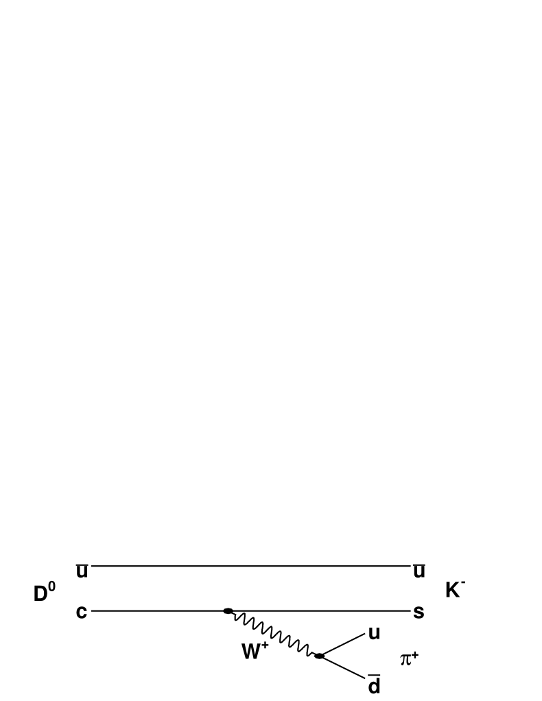
Figure 2: Quark diagram for $D^{0}\rightarrow{K^{-}\pi^{+}}$. The light $\bar{u}$ quark does not participate in the decay and is referred to as a “spectator”.

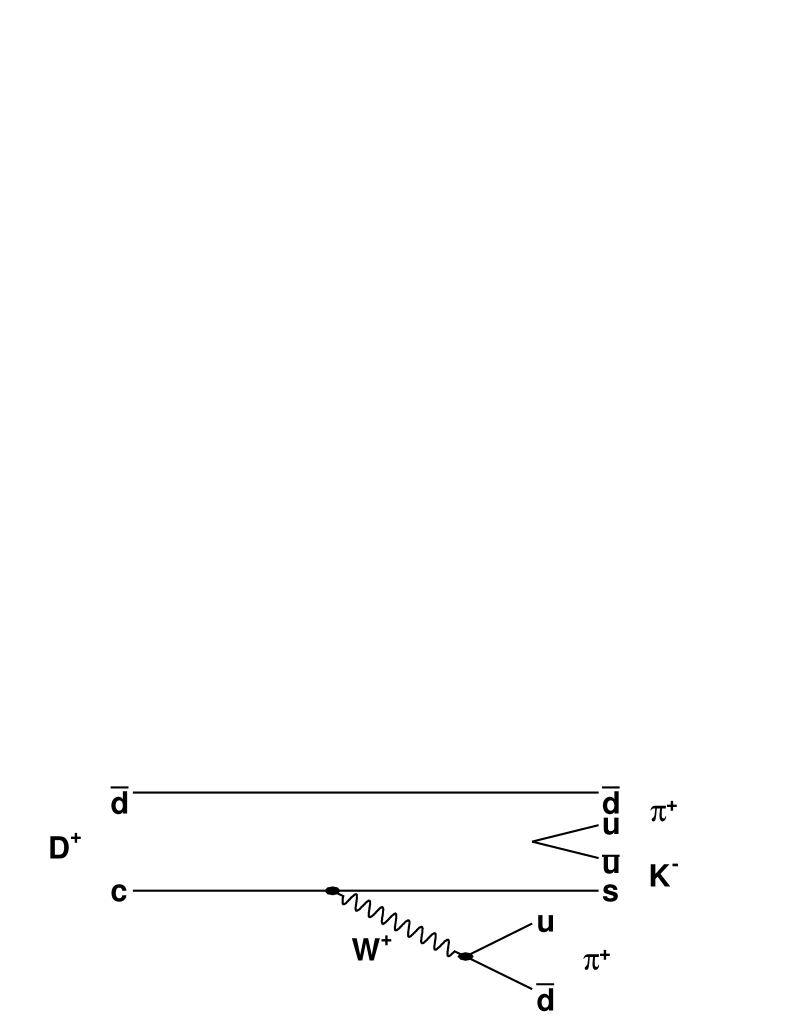
Figure 3: Quark diagram for $D^{+}\rightarrow{K^{-}\pi^{+}\pi^{+}}$. The light $\bar{d}$ quark does not participate in the decay and is referred to as a “spectator”.

The first detection of a $D$-meson decay was made by the Mark I collaboration [13] in the modes $D^{0}\rightarrow{K}^{-}\pi^{+}$, $D^{0}\rightarrow{K}^{-}\pi^{+}\pi^{-}\pi^{+}$, and ${D}^{+}\rightarrow{K}^{-}\pi^{+}\pi^{+}$. In addition to these charm mesons, the Mark I collaboration also observed the lowest charm-meson excited states of $D^{*0}$ and $D^{*+}$ [14].

In addition to a charm quark combining with an up or a down quark to form a meson, it can also combine with a strange quark to form what is referred to as a $D_{s}$ meson. The decay of this type of meson can be characterized by the conversion of the charm quark into a strange quark with an emission of a virtual $W$-boson. The simplest possible final products result when the newly-formed strange quark pairs with a strange quark to form a $\phi$ or an $\eta$ meson and the virtual $W$-boson forms a charged pion. Therefore, a search for an excess of $\eta\pi$ or $\phi\pi$ production would be evidence of $D_{s}$ mesons. The discovery of $D_{s}$ (initially called $F$) was presented by the CLEO collaboration in 1983 by observing a peak in the invariant mass spectrum for the decay mode $\phi\pi$ [15], following a period of considerable experimental uncertainty [16].

3 Motivation for this Measurement

The years following the charm discovery provided few opportunities for its detailed study, especially the $D_{s}$. The CLEO-c experiment was proposed in 2001 as to provide the first high-statistics study of charmed particles with a state-of-the–art detector. Initial CLEO-c running beginning in late 2003, focused on studies of $D^{0}$ and $D^{+}$, with the expectation that $D_{s}$ studies would follow.

From August until October 2005, the CLEO-c collaboration carried out a scan of the center-of-mass energy range from 3970 to 4260 MeV. The main purpose of this scan was to determine the optimal running point for CLEO-c studies of $D_{s}$-meson decays. Secondary objectives included detailed measurements of the properties of charm production in this region, tests of previous theoretical predictions, and confirmation and additional studies of the $Y(4260)$ state reported by the BaBar collaboration [17]. In this dissertation, measurements with the scan data of the cross sections for inclusive hadron production, charmed-hadron production, and the production of specific final states including charmed mesons are presented. We present results both without and with radiative corrections. We also report initial studies with detailed features of these events and present comparisons with past measurements and theoretical expectations. All of which will add to our present understanding for systems containing heavy and light quarks.

3.1 Previous Experimental Results

The total hadronic cross section in $e^{+}e^{-}$ annihilations is generally presented in terms of $R$, which is defined as follows:

$$R=\frac{\sigma(e^{+}e^{-}\rightarrow{hadrons})}{\sigma(e^{+}e^{-}\rightarrow\mu^{+}\mu^{-})}.$$ (1)

Incorporating the well-known $\mu$-pair cross section with its $1/s$ energy dependence gives

$$\sigma(e^{+}e^{-}\rightarrow{hadrons})=R\sigma(e^{+}e^{-}\rightarrow\mu^{+}\mu^{-})=R\frac{86.8{\rm{~{}nb~{}GeV}}^{2}}{E_{\rm{cm}}^{2}}.$$ (2)

If strong interactions are ignored:

$$R=3\sum_{i}q^{2}_{i}$$ (3)

where the summation is over all kinematically allowed quark flavors at the energy of interest, $q_{i}$ is the quark’s corresponding charge (either $-1/3$ or $2/3$), and the factor are 3 is due to the fact that there is 3 different colors available. This approximation only holds in energy regions well above the $q\bar{q}$ bound states.

Equation 1, counts the number of possible quarks that are available at a particular energy. In the energy region below, the $J/\psi$ resonance, $M_{J/\psi}=3.097$ [2], only the $u,~{}d,$ and $s$ quarks contribute to $R$:

$$R=3[(\frac{2}{3})^{2}+(\frac{1}{3})^{2}+(\frac{1}{3})^{2}]=2$$ (4)

Above this energy the $c$ quark can also contribute to the ratio.

$R$ has been measured over a very wide energy range by many experiments [2], including recent measurements with the Beijing Spectrometer (BES) [18] in the energy range of interest for CLEO-c. Fig. 4 shows the current state of knowledge of $R$ at center-of-mass energies between 3.2 and 4.4 GeV.

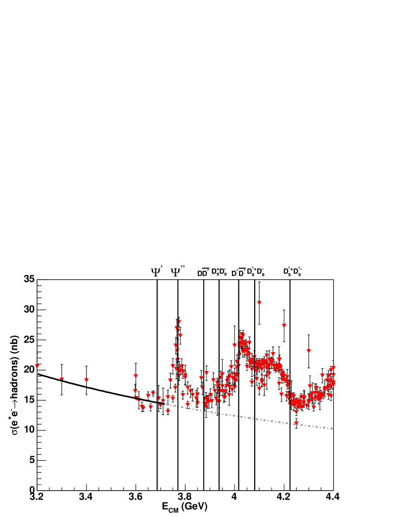
Figure 4: $\sigma(e^{+}e^{-}\rightarrow{hadrons})$ from the 2005 PDG [2]. The solid line is a $\frac{1}{s}$ fit to the data and the dotted line is the extension of the fit to higher energies. The vertical lines indicate the various thresholds and resonances present in the region.

The data in Fig. 4 has been radiatively corrected. The correction depends on the center-of-mass energy and the behavior of the cross section at lower energies. There is a rich structure in this energy region, reflecting the production of $c{\bar{c}}$ resonances and the crossing of thresholds for specific charmed-meson final states. Some of these “landmarks” are highlighted with vertical lines in Fig. 4. The specific energies corresponding to these thresholds are tabulated in Table 4.

Table 4: Thresholds of interest in the $e^{+}e^{-}$ center-of-mass energy range of the CLEO-c scan. Threshold values are computed from the PDG [2], and where needed charged and neutral states of the $D$ were averaged.

Center-of-Mass	3875 MeV	3937 MeV	4017 MeV	4081 MeV	4224 MeV
Energy
State	$D^{*}\bar{D}$	$D_{s}\bar{D}_{s}$	$D^{*}\bar{D}^{*}$	$D_{s}^{*}\bar{D}_{s}$	$D_{s}^{*}\bar{D}_{s}^{*}$

There are two interesting features in the hadronic cross section between 3.9 and 4.2 GeV. There is a large enhancement at $\sim 4$ GeV corresponding to the $D^{*}\bar{D}^{*}$ threshold. Next, there is a fairly large plateau that begins at the $D_{s}^{*+}D_{s}^{-}$ threshold. There is considerable theoretical interest and little experimental information about the specific composition of these enhancements.

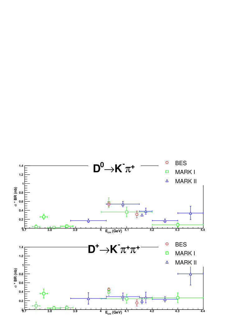
Figure 5: The production cross section times branching ratio for $D^{0}\rightarrow{K^{-}\pi^{+}}$ and $D^{+}\rightarrow{K^{-}\pi^{+}\pi^{+}}$ as a function of energy.

Prior to the CLEO-c scan run there were insufficient data on $D_{s}$ production for an informed decision about the best energy at which to undertake CLEO-c studies of $D_{s}$ decays. BES measured the inclusive $D_{s}$ production cross section times the $D_{s}^{+}\rightarrow{\phi}\pi^{+}$ branching ratio at the center-of-mass energy $4030$ MeV to be ($11.2\pm 2.0\pm 2.5$) pb [19]. Since there is only one accessible final state with $D_{s}$ at this energy, this measurement suggested a cross section of about 0.3 nb for $D_{s}^{+}{D}_{s}^{-}$. The Mark III collaboration previously measured the same quantity at a center-of-mass energy of $4140$ MeV to be ($26\pm 6\pm 5$) pb [20]. $D_{s}$ production had previously been demonstrated to be dominated at this energy by $D^{*+}_{s}D_{s}^{-}$ [21]. The ability to do $D_{s}$ physics with CLEO-c depends both on the quantity of $D_{s}$ production and on the complexity of the events. It was therefore essential to measure all accessible final states and carefully assess the physics reach for future $D_{s}$ studies under the conditions prevailing at each energy.

Studies of $D_{s}$ production, when combined with measurements of $D^{0}$ and $D^{+}$ production, would constitute a comprehensive analysis of all charm production in the region just above threshold. There are more previous measurements of $D^{0}$ and $D^{+}$ production than of $D_{s}$, but here too the information is limited. BES and MARK II made measurements of cross section time branching ratio for $D^{0}\rightarrow{K^{-}\pi^{+}}$ and $D^{+}\rightarrow{K^{-}\pi^{+}\pi^{+}}$ [22, 23, 24, 25], which are shown in Fig. 5. Interpretation of these data points is complicated by the presence of several possible final states: $D\bar{D}$, $D^{*}\bar{D}$, and $D^{*}\bar{D}^{*}$ in both charged states. Strong interaction theory provides predictions of the overall cross sections and proportions of the various final states, some of which are described in the next section. Detailed measurements at several points would allow more rigorous testing of models of charm production in the region above $c\bar{c}$ threshold.

3.2 Theoretical Predictions

Soon after the discovery of the $D$ meson relative production ratios were predicted by counting available spin states [26] for the possible reactions:

• $1^{-}\rightarrow{0^{-}0^{-}}$, as in $e^{+}e^{-}\rightarrow\gamma^{*}\rightarrow{D\bar{D}}$

• $1^{-}\rightarrow{0^{-}1^{-}}$, as in $e^{+}e^{-}\rightarrow\gamma^{*}\rightarrow{D\bar{D}^{*}}$

• $1^{-}\rightarrow{1^{-}1^{-}}$, as in $e^{+}e^{-}\rightarrow\gamma^{*}\rightarrow{D^{*}\bar{D}^{*}}$

This argument gives thefollowing ratios:

$$\sigma_{D\bar{D}}:\sigma_{D^{*}\bar{D}}:\sigma_{D^{*}\bar{D}^{*}}=1:4:7$$ (5)

This naive expectation disagrees with the experimentally observed ratios obtained by the Mark I experiment [14] at 4028 MeV:

$$\sigma_{D\bar{D}}:\sigma_{D^{*}\bar{D}}:\sigma_{D^{*}\bar{D}^{*}}=0.2\pm 0.1:4.0\pm 0.8:128\pm 40,$$ (6)

where the $p^{3}$ phase space factor has been removed. The severe disagreement between what is expected and what is experimentally observed suggests that major additional effects are present.

A serious theoretical calculation of the charm cross sections was first attempted by Eichten et al. in 1980 [27] with a coupled-channel potential model. Their predictions for the excess $\Delta{R}$ above $uds$ production are shown in Figs. 6 and 7. According to these predictions the large enhancement in the cross section at $4030$ MeV is dominated by $D^{*}\bar{D}$ and $D^{*}\bar{D}^{*}$ production. A detailed investigation of this energy region could definitively confirm or refute this prediction.

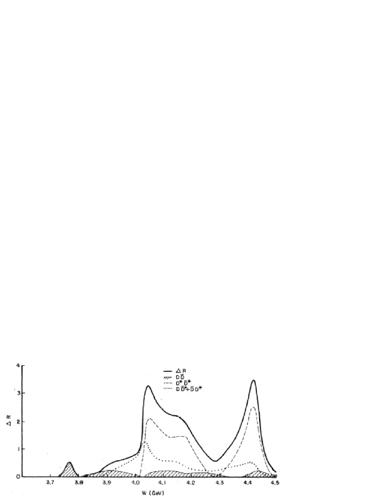
Figure 6: The charm contribution to $R$ as calculated in the coupled channel model of Eichten et al. [27] for $D^{(*)}\bar{D}^{(*)}$ events.

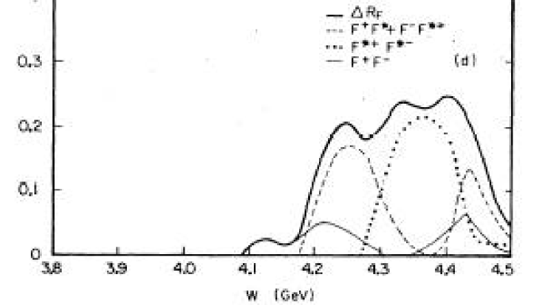
Figure 7: The $D_{s}$ contribution to R as calculated in the coupled channel model Eichten et al. [27] for $D^{(*)}\bar{D}^{(*)}$ of events. In the figure $D_{s}$ is called $F$.

The mass of the $D_{s}$ meson used in Eichten’s 1980 prediction is incorrect, as indicated by use of the older notation $F$ for that particle. To update Eichten’s prediction, it is therefore necessary to shift the cross sections downward in energy by $144$ MeV and $100$ MeV for $D_{s}^{+}D_{s}^{-}$ and $D_{s}^{*+}D_{s}^{-}$, respectively. After this correction, Eichten predicts that the largest $D_{s}$ yield should be at $\sim 4160$ MeV, where the dominant source is $D_{s}^{+}D^{*-}_{s}$ events.

More recently, T. Barnes [28] has presented calculations, using the phenomenological ${}^{3}P_{0}$ model [29], at 4040 and 4159 MeV, which are summarized in Table 5.

Table 5: Partial widths, in units of MeV, of charm production as predicted by Barnes for two center of mass energies.

Center-of-Mass	$D\bar{D}$	$D^{*}\bar{D}$	$D^{*}\bar{D}^{*}$	$D_{s}^{+}{D_{s}^{-}}$	$D^{*+}_{s}{D^{-}_{s}}$	SUM	Exp.
Energy
4040 MeV	0.1	33	33	7.8	-	74	52$\pm$10
4159 MeV	16	0.4	35	8.0	14	74	78$\pm$20

Of these two energy points, Barnes predicts that $4159$ MeV is the better place for $D_{s}$ physics, with a total cross section for $D_{s}$ production that is three times larger than that at $4040$ MeV. In addition, he finds the enhancement in $R$ at $\sim$4 GeV to be due to an equal mixture of $D^{*}\bar{D}$ and $D^{*}\bar{D}^{*}$ events. While the experimentally measured summed rate differs by $\sim 2\sigma$ from Barnes’s prediction at $4040$ MeV, the precision is insufficient for a definitive conclusion. Precise measurements of the partial widths with CLEO-c would be decisive in testing this model.

Chapter Experimental Apparatus

4 CESR - The Cornell Electron Storage Ring

The Cornell Electron Storage Ring, or CESR, is located in central New York on the Cornell University campus. As shown in Fig. 8, CESR consists of three basic parts: a linear accelerator (linac), a synchrotron, and the storage ring. The storage ring and synchrotron are housed in a circular tunnel which has a diameter of 244 meters. The linac is located in the inner part of the ring. The CLEO-c detector is located at the south end of the tunnel.

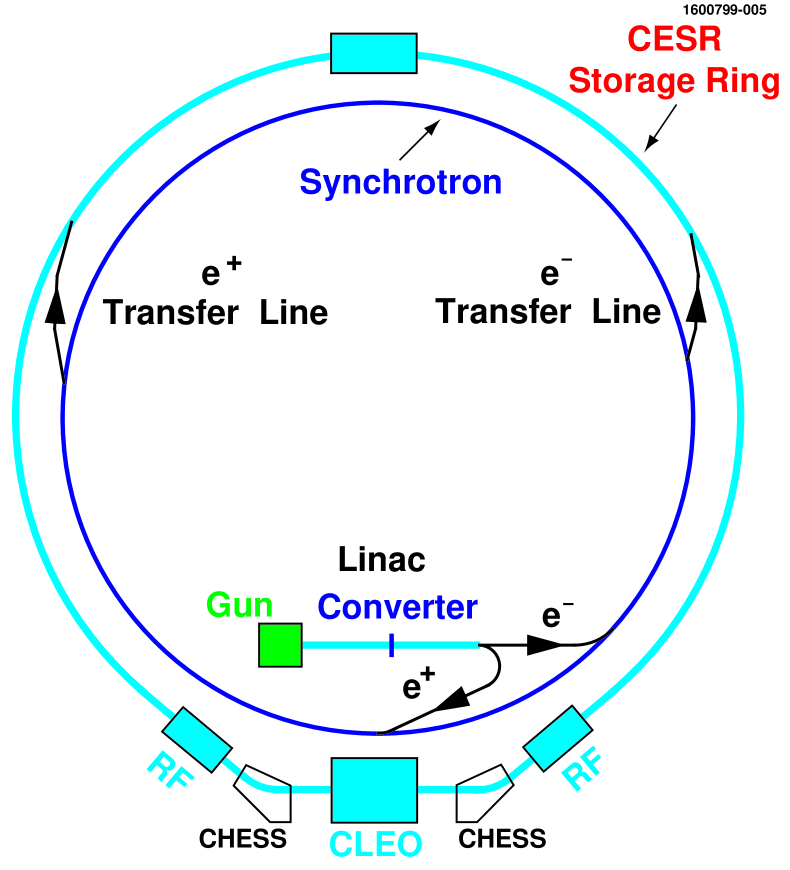
Figure 8: The CESR accelerator facility. The main components of the facility are the linac, the synchrotron, and the storage ring. The linac converter is a piece of tungsten used to induce an electromagnetic shower so as to produce positrons. CHESS refers to the Cornell High Energy Synchrotron Source.

Electrons for acceleration are created by boiling them off a heating filament. Once the energy is sufficient for them to escape from the surface, they are collected and bunched together for acceleration. The linac consists of oscillating electric fields which accelerate the electrons down the length of the linac. By the end, the electrons have an energy of approximately 200 MeV.

Positrons are created by inserting a tungsten target, a converter, halfway down the linac. The target is used to generate electromagnetic showers consisting of electrons, positrons, and photons. The positrons in the shower are selected out and accelerated the rest of the way down the length of the linac. By the end of the acceleration, the positrons reach an energy of 200 MeV.

The bunches of the electrons and positrons from the linac are injected separately and in opposite directions into the synchrotron. The synchrotron consists of a series of dipole magnets and four three-meter-long linear accelerating cavities. The dipole magnets steer the electrons and positrons around the ring while accelerating cavities increase the particles’ energies to about 2 GeV. As the energy of the particles increases the magnetic fields of the dipoles are increased to keep the particles in the ring. Once accelerated to 2 GeV, the electrons and positrons are transferred to the storage ring.

The storage ring consists of a series of a dipole magnets which steer the electrons and positrons around the ring, in addition to quadrupole and sextupole magnets which focus the beams. As the particles traverse the ring they lose energy due to synchrotron radiation. The energy is replaced by superconducting radio-frequency (RF) cavities which operate at a frequency of 500 MHz. These RF cavities are similar to those used in the linac and synchrotron, except that they do not significantly accelerate the beams, but primarily replace the radiated energy.

In current running conditions, CESR operates with nine bunch trains each for the electrons and positrons. Each train consists of as many as five bunches. To avoid unwanted interactions with the two counter-rotating beams four electrostatic horizontal separators are used. These separators set up what are known as pretzel orbits and ensure that the electrons and positrons miss each other when they pass through the unwanted intersecting locations, sometimes referred to a parasitic crossing. A picture showing an exaggerated view of the pretzel orbits is shown in Fig. 9. At the interaction point, which is surrounded by the CLEO-c detector, the two beams are steered into each other. However, the two beams do not collide head-on, but rather at a small crossing angle of 2.5 mrad ($\approx 1.7^{o}$). This allows for bunch-by-bunch interactions of the electron and positron trains.

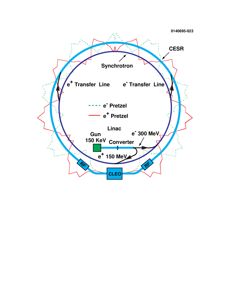
Figure 9: Schematic of CESR showning the “pretzel” orbits. The pretzel orbits are used to separate the electron and positron beams at parasitic crossing locations.

Between 1979 and 2003, CESR operated at the $\Upsilon(4S)$ resonance, which corresponds to a center-of-mass energy of 10.6 GeV or beam energy of 5.3 GeV. The CLEO-c charm program is carried out at center-of-mass energies between 3 and 5 GeV, which required major changes to CESR. The rate of synchrotron radiation, energy radiated by the beams due to acceleration by the bending magnets, is proportional to $E^{4}$ [30]. The decrease in the amount of synchrotron radiation affects storage ring performance through two important beam parameters. One is the damping time with which perturbations in beam orbits caused by injection and other transitions decay away. In particular, a particle that is off the ideal orbit because of a larger energy radiates slightly more energy, whereas a particle with a lower energy radiates slightly less. As a whole, the energy spread among the particles becomes reduced which shows up as a damping of the oscillations [31]. In the original CESR design the radius was chosen to ensure adequate damping through this mechanism at a 5-GeV beam energy. Since the amount of radiation is dependent upon the energy of the corresponding particles in the beam, with a reduction in beam energy to $\sim{2}$ GeV, the damping time becomes too long for effective operation. The other parameter is the horizontal beam size, or horizontal emittance, which measures the spread of particles in the bend plane. The horizontal beam size, which results from the betatron oscillation in addition to the rate of quantum fluctuations in the synchrotron radiation, decreases with decreasing beam energy thereby limiting the particle density per bunch [31].

These effects limited the achievable collision rate (luminosity) of CESR at the lower center-of-mass energies of CLEO-c to unacceptable levels. To increase the luminosity CESR accelerator physicists proposed to increase the amount of radiation through the use of wiggler magnets [30].

A wiggler magnet is a series of dipole magnets with high magnetic fields. Each successive dipole has its direction of magnetic field flipped. Therefore, when a particle passes, it will oscillate, which results in emission of additional synchrotron radiation without changing the overall path of the particle around the ring. As a result, the damping time is decreased while the horizontal beam size is increased, thereby increasing the luminosity.

CESR has installed twelve superconducting wiggler magnets for low-energy running. Each wiggler consists of eight dipole magnets with a maximum field strength of 2.1 Tesla [30]. These wigglers decrease the damping time by a factor of 10, while increasing the beam emittance by a factor of 4 to 8 [32]. In addition, the energy resolution has increased, as compared to no wigglers, by a factor of 4 to $\sigma_{E}/E=8.6\times 10^{-4}$ [32].

The center-of-mass (CM) energy of the collision is an important quantity needed to put the cross section measurements into context. In order to determine the CM energy of the colliding electrons and positrons, one needs to know the energy of the beams. The energy of the beams, to first order, can be determined by the following [33]:

$$E_{o}=\frac{ec}{2\pi}\sum_{i}|B_{i}|\Delta\theta_{i}\rho_{i},$$ (7)

where $c$ is the speed of light in a vacuum and $e$ is the charge of an electron. The summation in Eq. 7 is over all dipole magnets in the ring, where $B_{i}$, $\theta_{i}$, and $\rho_{i}$ are the magnitude of the magnetic field, the bending angle, and bending radius of curvature of the $i$-th dipole magnet, respectively. The result of Eq. 7 needs to be corrected for shifts in RF accelerating cavities, for the currents of the the focusing and steering magnets, and for the horizontal separators. The total uncertainty in the CM energy is of order 1 MeV.

Another quantity needed in determining the cross sections is the luminosity, which quantifies the rate of $e^{+}e^{-}$ collisions. The number of events expected for a particular process is given by

$$N_{i}=\sigma_{i}\int{\cal{L}}dt,$$ (8)

where $\cal{L}$ is the instantaneous luminosity and $\sigma_{i}$ is the cross section for that process. The integral of the instantaneous luminosity, $\int{\cal{L}}dt={\rm{L}}$, is the quantity needed for this analysis and is referred to as the integrated luminosity or just luminosity. In CLEO-c, three final states are used to obtain the luminosity. The processes $e^{+}e^{-}\rightarrow{e^{+}e^{-}}$, $\mu^{+}\mu^{-}$, and $\gamma\gamma$ are used since their cross sections are precisely determined by QED. Each of the three final states relies on different components of the detector, with different systematic effects [34]. The three individual results are combined using a weighted average to obtain the luminosity needed for this analysis.

5 The CLEO-c Detector

The electron and positron beams are steered into each other at the central location known as the interaction point (IP) of the CLEO-c detector. CLEO-c is a general-purpose detector designed to identify and measure relatively long-lived charged and neutral particles. The charged particles detected are the electron, muon, pion, kaon, and proton. While some neutral particles are easy to identify, like the photon, others like the neutrinos are impossible.

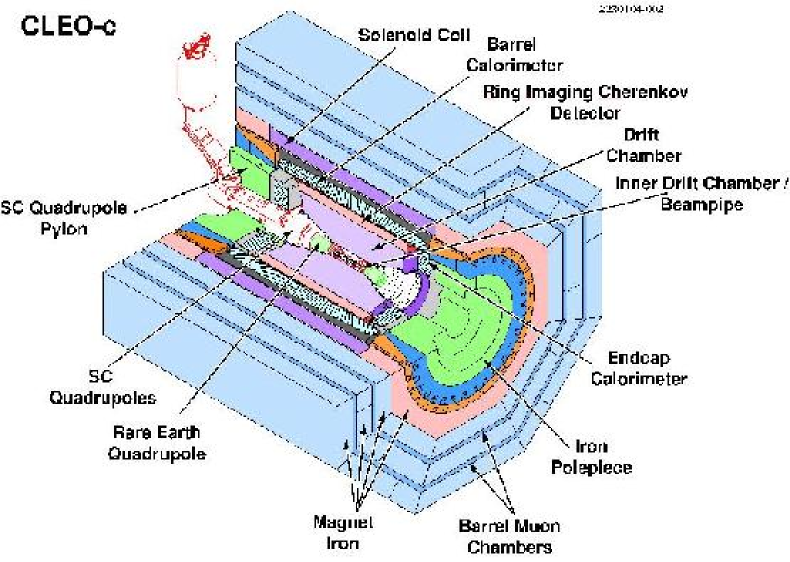
Figure 10: The CLEO-c detector.

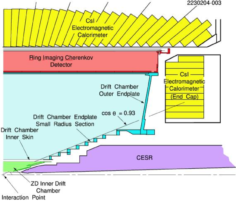
Figure 11: A slice in the r-z plane of the CLEO-c detector.

The remainder of this chapter is dedicated to describing the detection systems that make up the CLEO-c detector. As shown schematically in Figs. 10 and 11, CLEO-c is a cylindrically symmetric detector aligned along the beam line, the z-axis, that covers 93% of the solid angle. Starting from the IP and moving out, the detector is composed of an inner drift chamber [30], an outer or main drift chamber [30, 35], a Ring-Imaging Cherenkov detector [30, 36, 37], denoted by the acronym RICH, a crystal calorimeter [30, 38], and finally a muon detector [30, 38, 39]. All systems, except for the muon detector, are within a uniform 1-Tesla magnetic field, produced by a superconducting solenoid, which is aligned with the beam axis.

5.1 Inner Drift Chamber

The inner drift chamber (ZD) is the innermost detector of CLEO-c, located right outside the beam pipe. The inner drift chamber replaced the silicon vertex detector of CLEO III because multiple scattering degrades the momentum resolution for soft tracks, which are more prevalent at low center-of-mass energies. Therefore, minimizing the material is crucial. The goal of the detector is to detect charged particles with $|\cos\theta|<0.93$, where $\theta$ is defined as the angle of the particle with respect to the beam pipe, the z-axis. It consists of helium-propane-gas-filled volume segmented into 300 cells (half-cell size of 5 mm), where each cell consists of a sense wire held at +1900 V. These cells are surrounded by field wires, held at ground, which neighboring cells share. When a charged particle travels through a cell the gas is ionized. The resulting ionized electrons travel away from the field wire and toward the sense wire. Since the electric field increases close to the sense wire, the primary electrons will ionize other atoms in the gas, thereby creating an avalanche of electrons at the sense wire. The time of the resulting electric pulse seen on the sense wire, which is synchronized with the bunch crossing, is converted using the drift velocity of the gas to a distance of closest approach to the sense wire. This information can then be used to map out the trajectories of the charged particles through the drift chamber.

5.2 Outer Drift Chamber

Located directly outside the inner drift chamber is the main drift chamber, sometimes referred to as the outer drift chamber (DR). The main drift chamber has a similar design to the ZD, except that it is larger in size both overall, with 47 layers of field and sense sires as compared to 6 for the ZD, and in the size of the cell, with a half-cell size of 7 mm as compared to 5 mm. In addition, the field wires are held at a higher potential, +2100 V rather than +1900 V.

The energy lost by a charged particle in the drift chamber is used in identifying what particle traversed the volume. The energy lost per unit length, $dE/dx$, is related to the particle’s velocity. By constructing a $\chi^{2}$-like variable, the consistency of the actual energy lost per unit length with what is expected for different particle hypotheses can be assessed:

$$X_{i}=\frac{dE/dx^{measured}-dE/dx^{expected}_{i}}{\sigma},$$ (9)

where $i$ = $e,~{}\mu,~{}\pi,~{}K,$ or $p$. The quantity $\sigma$ is the uncertainty in the measurement, usually approximately 6%. Fig. 12 shows the measured $dE/dx$ as a function of particle momentum for a large number of charged particles detected in CLEO-c. The figure clearly shows good $\pi-K$ separation for momenta below 500 MeV. At momenta above 500 MeV, $dE/dx$ is quite limited and the additional separation power of the RICH is needed.

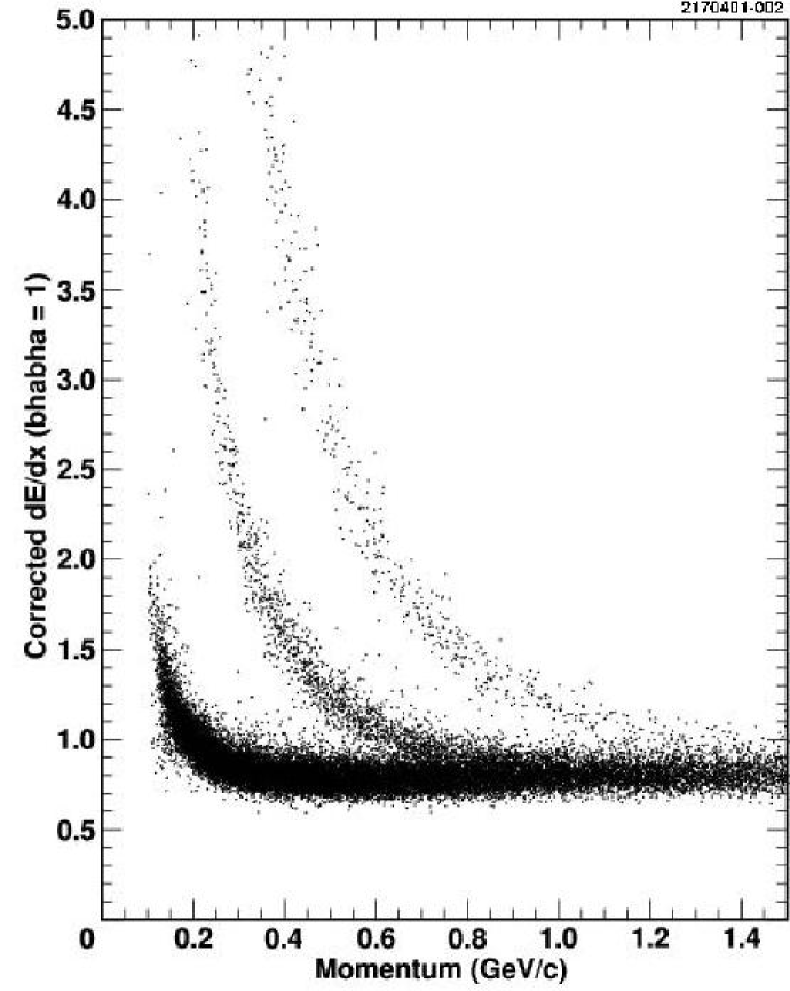
Figure 12: $dE/dx$ as a function of momentum for a large population of charged particle measured in CLEO-c. The $\pi,~{}K$, and $p$ bands, from left to right, are clearly seen.

As mentioned earlier, the ZD and DR are contained inside a 1-Telsa magnetic field oriented along the beam. This field causes charged particles to travel in helical paths as they travel through the detector volume. In other words, the particle’s path is circular in the x-y plane and moves with constant velocity along the z-axis. Pattern recognition computer programs group the hits into tracks and fitting programs are used to obtain the parameters [40]. The CLEO-c fitter is an implementation of the Billoir or Kalman algorithm, which incorporates the expected energy loss of a particular particle to optimize the determination of its momentum and trajectory. At 1 GeV$/c$ the charged-particle momentum resolution is approximately 0.6%.

5.3 RICH - Ring Imaging Cherenkov Detector

Directly outside the main drift chamber is the Ring Imaging Cherenkov Detector, commonly referred to as the RICH. Radiation is emitted when a charged particle’s velocity is greater than the speed of light in the medium through which the particle is traveling; this radiation is known as Cherenkov radiation. The radiation is emitted in a cone with a characteristic opening angle known as the Cherenkov angle. The Cherenkov angle is related to the velocity of the particle by

$$\cos\theta=\frac{1}{\beta{n}},$$ (10)

where $\beta$ is the velocity in units of $c$ and $n$ is the index of refraction of the medium. Using $\beta=\frac{p}{E}$, in addition to $E^{2}=m^{2}+p^{2}$, Eq. 10 can be rewritten in terms of the particle’s mass and momentum as follows:

$$\cos\theta=\frac{1}{n}\sqrt{1+\frac{m^{2}}{p^{2}}}.$$ (11)

This shows that one can identify the type of particle by using its momentum from the fitted track and the observed Cherenkov angle.

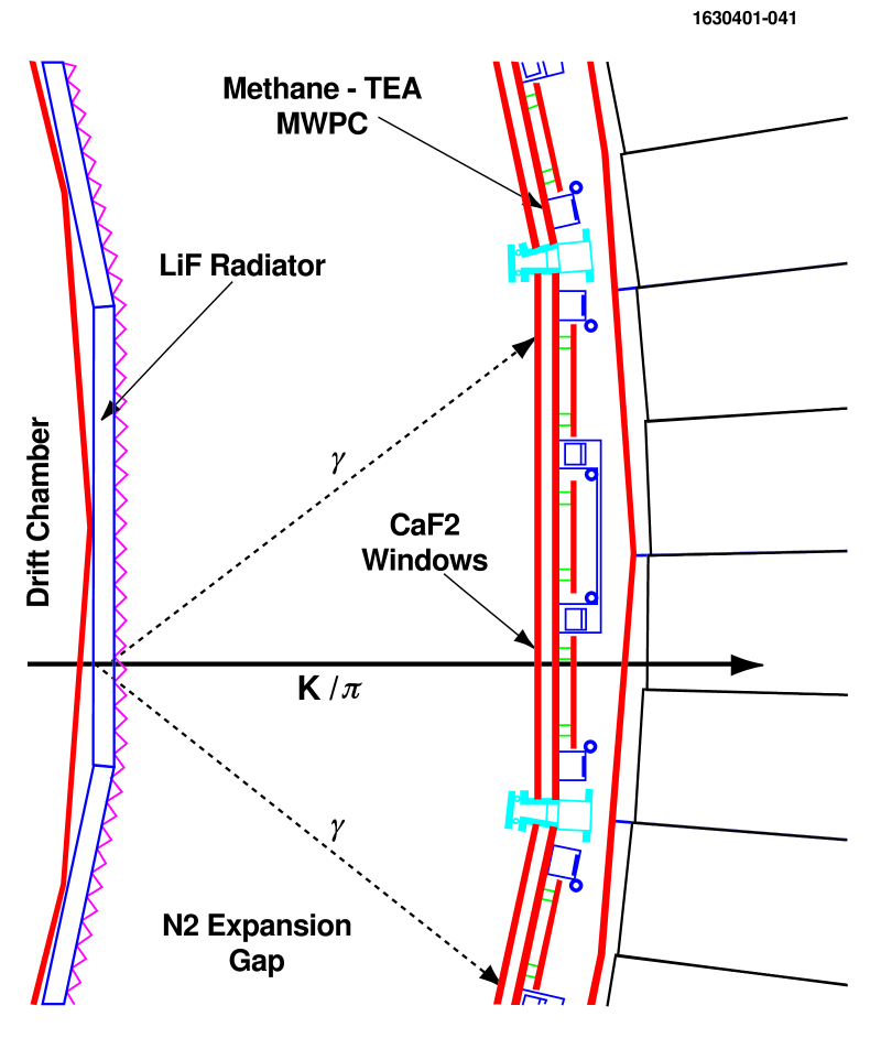
Figure 13: A section of the CLEO-c RICH detector shown in $r-\phi$ cross section.

The RICH detector is shown schematically in Fig. 13. It covers approximately 83% of the full 4$\pi$ solid angle. Cherenkov photons are produced when a charged particle passes through entrance windows fabricated from LiF crystals, as shown in Fig. 13. There are a total of 14 rows, or rings, of these radiator crystals. All but the central four have flat surfaces, while the remainder have a “sawtooth” surface to reduce loss of photons by total internal reflection. The photons, which have a typical wavelength $\lambda=150$ nm, travel through an expansion volume filled with nitrogen gas which is effectively transparent. After traveling through the expansion volume they pass through a CaF₂ window and into a multi-wire proportional chamber (MWPC) filled with a methane-TEA (tri-ethyl amine) mixture. Here photoelectrons are created which are collected in the same manner as described above for the drift chambers. Examples of the Cherenkov rings are shown in Fig. 14.

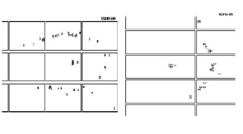
Figure 14: Cherenkov rings produced by a charged track for the flat radiator (right) and sawtooth (left). The central hits of each image are due to the charge track passing through the wire chamber. The other hits are due to the Chernkov photons that are produced. Half of the image of the flat radiator is missing because it was trapped in the radiator by total internal reflection. The sawtooth imagine is distorted by refraction.

Using Cherenkov photon images, like those in Fig. 14, one can construct the likelihood for a particular particle hypothesis. A $\chi^{2}$-like variable for identification can be constructed to discriminate between two different particle hypotheses:

$$\chi_{i}^{2}-\chi_{j}^{2}=-2\ln{L_{i}}+2\ln{L_{j}},$$ (12)

where $L_{i}$ and $L_{j}$ are the likelihoods for particle hypotheses $i$ and $j$, respectively. An illustration of the power of the RICH detector is shown in Fig. 15. Requiring $\chi^{2}_{K}-\chi^{2}_{\pi}<0$, that is that the particle is more kaon-like than pion-like, and that momentum is greater than 700 MeV$/c$, leads to a kaon identification efficiency of 92% with a pion-fake rate of 8%. Fig. 16 shows particle separation as a function of momentum for different particle hypotheses above their respective thresholds, where the threshold is determined by the index of refraction of the LiF radiator, $n=1.4$.

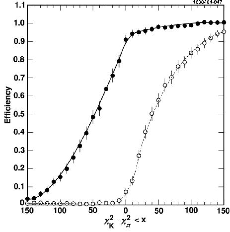
Figure 15: Kaon identification efficiency (solid points) and pion fake rate (open circles) as a function of various cuts on $\chi^{2}_{K}-\chi^{2}_{\pi}$. Momentum is restricted to be above 700 MeV/$c$.

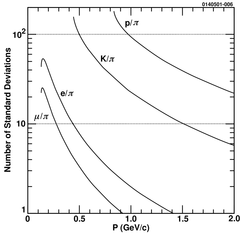
Figure 16: Particle separation as a function of momentum for different particle hypotheses in the RICH detector. Both particles are restricted to be above their respective threshold, where the threshold is determined by the index of refraction of the LiF radiator, $n=1.4$.

5.4 Calorimetry

Located just outside the RICH and just inside CLEO-c’s superconducting magnet is the electromagnetic crystal calorimeter (CC). The CC consists of about 7,800 thallium-doped cesium iodide crystals. About 80% of the crystals are arranged in a projective geometry in the barrel region, defined by $|\cos\theta|<0.8$. The remainder are in two end-caps, covering $0.85<|\cos\theta|<0.93$. The transition regions between the barrel and end-caps provide substandard performance and are generally not used.

When charged particles or photons enter these highly dense crystals they interact and lose energy through various mechanisms: ionization, bremsstrahlung, pair conversion, and nuclear interactions. Electromagnetic interactions with these high-Z nuclei are very effective in stopping electrons and photons. Hadrons, on the other hand, lose energy less quickly in the CC electromagnetically, and their hadronic showers extend into the steel of the flux return of the superconducting solenoid. Muons and noninteracting hadrons, which deposit only a small fraction of their energy inside the calorimeter, and are referred to as minimum ionizing particles (MIPS). While hadrons generally are absorbed in the steel, the muons continue to lose energy only by ionization and travel through the magnet and into the proportional chambers that comprise the muon detector.

Electrons and photons lose energy through the successive generation of bremsstrahlung photons and $e^{+}e^{-}$ production, together known as an electromagnetic shower. These showers produce numerous low-energy electrons which are then captured by the thallium atoms. The photons emitted by the de-excitation of thallium, $\lambda=560$ nm, are invisible to the rest of the crystal. This means, they can propagate through the rest of the 30 cm-long crystal and be collected by the photo-diodes mounted on the back of the crystal. The energy resolution is about 4.0% at 100 MeV and 2.2% at 1 GeV. The resolution of the total shower energy is increased when more than one crystal is used in the reconstruction. This can be seen in Fig. 17. The center of the shower is then determined by an energy-weighted average of the blocks used in the sum. The number of crystals used is logarithmic, and ranges from 4 at 25 MeV to 13 at 1 GeV.

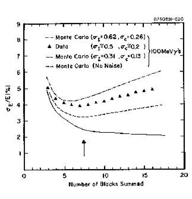
Figure 17: Shower energy resolution as a function of the blocks used in the shower reconstruction for the CLEO II detector. The barrel calorimeter has not changed since the installation of CLEO II. The smooth lines are from Monte-Carlo (MC) simulation of the 100 MeV photons. The points are experimental data from the 100 MeV transition photon in $\Upsilon(3S)\rightarrow\gamma\chi_{bJ}(2P)$. The arrow indicates the number of crystals used in the shower reconstruction of 100 MeV photons.

Figure 18: $M(\gamma\gamma)$ resolution in CLEO III.

5.5 Magnetic Field

CLEO-c’s 1-T magnetic field is provided by a large liquid-helium-cooled superconducting solenoid with a diameter of 3 m and length of 3.5 m. The resulting field produced is uniform to $\pm 0.02\%$ over the entire tracking volume. The iron flux return of the magnet is used in muon detection as an absorber, which is described next.

5.6 Muon Detection

The muon detector exploits the fact that muons do not participate in the strong interaction. Since muons are much heavier than electrons, they lose energy much more slowly as they travel through material. Therefore, muons can penetrate much greater depths of material. The detector consists of three layers of gas-filled, wire-proportional tracking chambers in between 36 cm iron absorbers surrounding the detector (see Fig. 19).

The muon detector’s layers provides information on a particle traveling different interaction lengths. The interaction length is the average distance a charged hadron has to travel before having an interaction. The three layers of the detector are located at approximately 3, 5, and 7 interaction lengths. Information from this detector is useful for identifying muons above about 1 GeV. Its applicability to the studies with CLEO-c reported in this thesis is limited.

Figure 19: Cross section of the muon chamber. It consists of three layers of 8-cell proportional counters. The middle counter layer is offset by one half a cell width to improve acceptance.

5.7 Data Acquisition

During the CLEO-c scan, bunch crossings happened at a rate on the order of 1 MHz. However, the actual rate of interesting physics events was much smaller, on the order of 1 Hz.

The CLEO-c detector includes hundreds of thousands of sensitive components and associated electronic channels. At every crossing each one of these components can deliver a signal representing the traversal of a particle produced in the $e^{+}e^{-}$ annihilation, although in typical events only a small fraction of these events have valid data. In general data are read out locally and “sparsified” to eliminate uninteresting channels. The nontrivial information is read out to on-line computers in tens of microseconds. During the data-gathering process, the detector can not acquire any new events. Because of this, it is essential to record only those events that contain interesting physics. This amount of “dead-time” is defined as the time between the trigger signal and the end of the digitization process. The maximum readout-induced dead-time is $<3\%$ [30].

Table 6: Definitions of the trigger lines.

Name	Definition
Hadronic	$(N_{axial}>1)\&(N_{CBlow}>0)$
Muon Pair	two back-to-back stereo tracks
Barrel Bhabha	back-to-back high showers in CB
End-cap Bhabha	back-to-back high showers in CE
Electron track	$(N_{axial}>0)\&(N_{CBmed}>0)$
Tau	$(N_{stereo}>1)\&(N_{CBlow}>0)$
Two Track	$(N_{axial}>1)$
Random	random 1 kHz source

The selection of these interesting physics events is achieved with a multi-layered trigger system [30, 41, 42, 43]. A schematic view of the CLEO-c trigger system is shown in Fig. 21. Currently, there are eight trigger lines used, listed in Table 6. Data from the DR and the CC are received and processed in separate VME crates and yield basic trigger parameters. These parameters are tracks counts, or multiplicity, topology in the main drift chamber, and the number of showers and topology in the calorimeter. The information from both systems is correlated by a global trigger which generates a “pass” signal every time a valid trigger condition is satisfied. The trigger system consists of two tracking triggers, one using information provided by the axial wires and the other using the stereo wires of the DR, a CC trigger, and a decision and gating global trigger system.

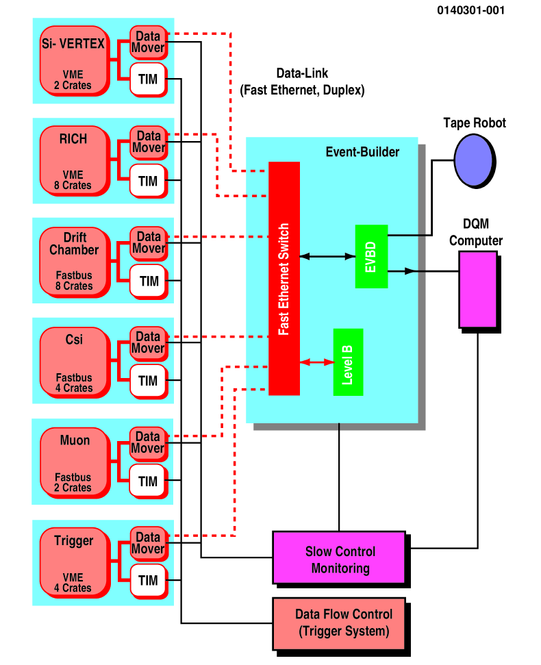
Figure 20: Block diagram of the CLEO III data acquisition system (DAQ). The only difference in the between CLEO III and CLEO-c detectors, and in turn the DAQ system is the replacement of the silicon vertex detector with the inner drift chamber.

The data acquisition system (DAQ) consists of two equally important parts. The DAQ system is responsible for the transfer of the data from the front end electronics to the mass storage device, while the slow control monitors environmental conditions, the quality of the data, and the status of detector components.

For each acceptable trigger from the CLEO-c detector, about 400,000 channels are digitized. The front-end electronics provide the data conversion in parallel with a local buffer and waits for an asynchronous readout by the DAQ. A dedicated module, the Data-Mover, in each front-end crate, assures transfer times of the data are below 500 $\mu{s}$, in addition to providing another buffer. The Data-Mover moves the data to the Event-Builder which reconstructs the accepted events for transfer to mass storage. Also, a fraction of reconstructed events are analyzed on-the-fly by the CLEO monitoring system, commonly referred to as Online-Pass1, to quickly discover problems and check the quality.

In addition to Online-Pass1, there is an Offline-Pass1, which is commonly referred to as Caliper (which stands for CALIbration and PERformance monitoring). Caliper, unlike Online-Pass1, can be run over all the data in an efficient manner by applying harsh cuts to get at the interesting physics events for data quality and monitoring. As a result, Caliper was used extensively during the scan running used for the analysis in this thesis.

A block diagram of the DAQ for the CLEO III detector is shown in Fig. 20. The only difference between the CLEO III and the CLEO-c detector, and that of the DAQ, is the replacement of the silicon vertex detector within the inner drift chamber.

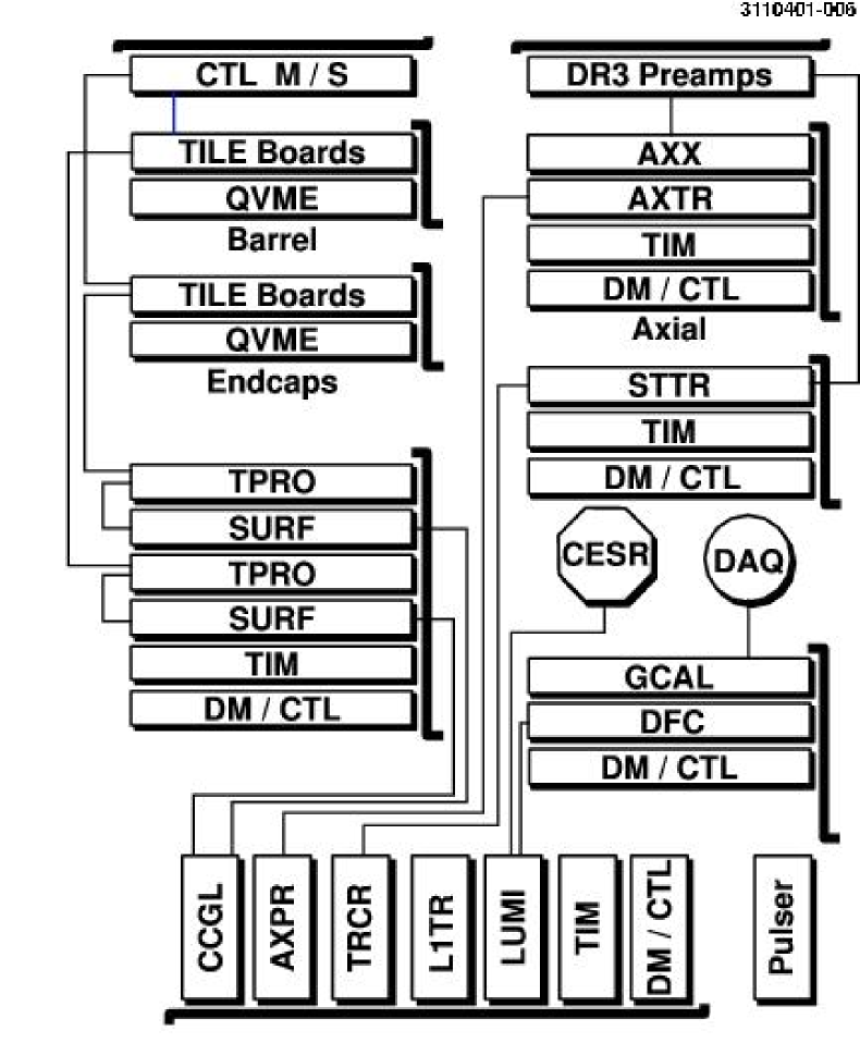
Figure 21: Overview of the trigger system.

Chapter CLEO-c $D_{s}$ Scan

The CLEO-c project description (Yellow Book) [30] includes measurements of $D_{s}$ branching fractions and other properties among the principal goals of the program. It makes a specific proposal that a scan run be undertaken to determine the running energy above $D_{s}^{+}D_{s}^{-}$ threshold that will maximize the sensitivity for $D_{s}$ physics. It also acknowledges that such a data sample would include non-strange charmed mesons in the form of $D\bar{D}$, $D^{*}\bar{D}$ and $D^{*}\bar{D}^{*}$ events produced in different quantum states from those at the $\psi(3770)$. It is on this scan data that this thesis is based.

6 Data and Monte Carlo Samples

The scan run was designed to provide maximum information in the available running period of August-October, 2005. The objective at each energy point was a measurement of the cross sections for all accessible final states consisting of a pair of charmed mesons. At the highest energy the possibilities include all of the following: $D\bar{D}$, $D^{*}\bar{D}$, $D^{*}\bar{D}^{*}$, $D_{s}\bar{D}_{s}$, $D_{s}^{*}\bar{D}_{s}$, and $D_{s}^{*}\bar{D}_{s}^{*}$, where the first four include both charged and neutral states. The original plan for the scan included ten energy points, with an integrated luminosity target for each point of $\sim 5$pb^-1. It was recognized that specific energies might reveal themselves as unpromising with less than this luminosity. The plan was therefore designed to be flexible, with the option of adding or revisiting points to the extent that the data suggested and time allowed. In the end two points were added to the original list, including one at 4260 MeV to investigate the $Y(4260)$. The center-of-mass energies and integrated luminosities for the twelve scan points are given in Table 7 and Fig. 22. An additional point was added as a result of the scan and corresponds to the location that maximizes the $D_{s}$ yield. This point, 4170 MeV, is added to this analysis and its larger data sample was essential in understanding the nature of charm production throughtout this energy region.

Table 7: Center-of-mass energies and integrated luminosities for all data points in the CLEO-c $D_{s}$ scan.

$\sqrt{s}$ (MeV)	${\int\cal{L}}dt$ (nb-1)
$3970$	$3854.30\pm 8.48$
$3990$	$3356.45\pm 7.73$
$4010$	$5625.65\pm 10.20$
$4015$	$1470.35\pm 5.32$
$4030$	$3005.55\pm 7.48$
$4060$	$3285.65\pm 7.79$
$4120$	$2759.20\pm 7.29$
$4140$	$4871.85\pm 9.77$
$4160$	$10155.40\pm 13.96$
$4160$	$178942.15\pm 59.37$
$4180$	$5666.90\pm 10.51$
$4200$	$2809.90\pm 7.59$
$4260$	$13107.60\pm 16.45$

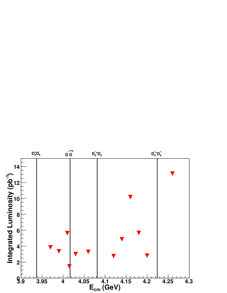
Figure 22: Integrated luminosity as a function of energy: The two largest integrated luminosity points correspond to 4160 and 4260 MeV. A point corresponding to 4170 MeV is left off, but has a luminosity of about 178 pb^-1

Numerous Monte Carlo (MC) samples have been generated in the development of the procedures and the determination of efficiencies and backgrounds for this analysis. The goal in specifying these MC samples was not to reproduce reality precisely, but to include all relevant final states in sufficient quantity to develop selection criteria and assess the potential for cross-feed backgrounds. Thirteen 100 pb^-1 samples (one for each center-of-mass energy), both signal and continuum, were generated. At each energy the signal MC sample includes all kinematically allowed $D_{(s)}^{(*)}\bar{D}_{(s)}^{(*)}$ final states. The continuum samples included only the $uds$ background. All MC samples for the scan were generated on a system of $\sim 50$ computers operated by the Minnesota CLEO-c group (“MN MC farm”). A breakdown of the signal MC samples is shown in Table 8. Additional samples, described later, were subsequently produced to aid in assessing the potential contributions of “multi-body” production.

Table 8: Composition of the $100$ pb^-1 signal MC samples. The assumed total charm cross section was $11$ nb for $E_{\rm{cm}}=4015-4200$ Mev and $5$ nb for $E_{\rm{cm}}=3970-4015$ and $4260$ MeV.

Event	3970	4015	4020-4080	4080-4200	4260
$D^{0}\bar{D^{0}}$	$11.6\%$	$6.9\%$	$6.9\%$	$6.6\%$	$6.3\%$
$D^{+}{D^{-}}$	$11.6\%$	$6.9\%$	$6.9\%$	$6.6\%$	$6.3\%$
$D^{*0}\bar{D^{0}}$	$35\%$	$13.7\%$	$13.7\%$	$13.2\%$	$12.6\%$
$D^{*+}{D^{-}}$	$35\%$	$13.7\%$	$13.7\%$	$13.2\%$	$12.6\%$
$D^{*0}\bar{D^{*0}}$	$-$	$54.9\%$	$27.4\%$	$26.4\%$	$25.1\%$
$D^{*+}{D^{*-}}$	$-$	$-$	$27.4\%$	$26.4\%$	$25.1\%$
$D_{s}^{+}D_{s}^{-}$	$7\%$	$4\%$	$4\%$	$2.5\%$	$1\%$
$D_{s}^{*+}D_{s}^{-}$	$-$	$-$	$-$	$5\%$	$2\%$
$D_{s}^{*+}D_{s}^{*-}$	$-$	$-$	$-$	$-$	$9\%$

7 Decay Modes and Reconstruction

Eight $D_{s}$ modes are used to measure the $D_{s}$ production at each energy point. These modes are listed in Table 9. In addition to these $D_{s}$ decays, several $D^{0}$ and $D^{+}$ decay modes, given in Table 10, were used to investigate the amount of $D\bar{D}$, $D^{*}\bar{D}$, and $D^{*}\bar{D}^{*}$ produced at each energy point.

Table 9: The $D_{s}$ branching fractions including the updated branching fractions, in $10^{-2}$.

Modes	Branching Fraction
$\phi\pi^{+}$, 10 MeV cut on the Invariant $\phi\rightarrow{K}^{+}K^{-}$ Mass [44]	$1.98\pm 0.15$
$K^{*0}K^{+},K^{*0}\rightarrow{K^{-}\pi^{-}}$ [2]	$2.2\pm 0.6$
$\eta\pi^{+},\eta\rightarrow{\gamma\gamma}$ [2, 44]	$0.58\pm 0.07$
$\eta\rho^{+},\eta\rightarrow{\gamma\gamma},\rho^{+}\rightarrow{\pi^{+}\pi^{0}}$ [2]	$4.3\pm 1.2$
$\eta^{{}^{\prime}}\pi^{+},\eta^{{}^{\prime}}\rightarrow{\pi^{+}\pi^{-}\eta},\eta\rightarrow{\gamma\gamma}$ [2, 44]	$0.7\pm 0.1$
$\eta^{{}^{\prime}}\rho^{+},\eta^{{}^{\prime}}\rightarrow{\pi^{+}\pi^{-}\eta},\eta\rightarrow{\gamma\gamma},\rho^{+}\rightarrow{\pi^{+}\pi^{0}}$ [2]	$1.8\pm 0.5$
$\phi\rho^{+},\phi\rightarrow{K^{+}K^{-}},\rho^{+}\rightarrow{\pi^{+}\pi^{0}}$ [2]	$3.4\pm 1.2$
$K_{s}K^{+},K_{s}\rightarrow{\pi^{+}\pi^{-}}$ [2, 44]	$1.0\pm 0.07$

Table 10: Decay modes used to select $D^{0}$ and $D^{+}$ in the scan data. The branching fractions are from a published CLEO-c analysis [45, 46].

Modes	Branching Fraction
$D^{0}$ decay mode
$K^{-}\pi^{+}$	$3.91\pm 0.12\%$
$K^{-}\pi^{+}\pi^{0}$	$14.94\pm 0.56\%$
$K^{-}\pi^{+}\pi^{+}\pi^{-}$	$8.29\pm 0.36\%$
$D^{+}$ decay mode
$K^{-}\pi^{+}\pi^{+}$	$9.52\pm 0.37\%$
$K^{-}\pi^{+}\pi^{+}\pi^{0}$	$6.04\pm 0.28\%$
$K_{s}\pi^{+}$	$1.55\pm 0.08\%$
$K_{s}\pi^{+}\pi^{0}$	$7.17\pm 0.43\%$
$K_{s}\pi^{+}\pi^{-}\pi^{+}$	$3.2\pm 0.19\%$
$K^{+}K^{-}\pi^{+}$	$0.97\pm 0.06\%$

In selecting these decays the CLEO-c standard DTAG [47] code was used with the following modifications to the usual criteria:

• The $\frac{dE}{dX}$ requirements for charged pions and kaons were relaxed from $3\sigma$ to $3.5\sigma$.

• The $K_{s}$ mass requirement was tightened from $4.5\sigma$ to $3\sigma$.

• The $\Delta E$ cut for tag selection was relaxed from $|\Delta E|<0.1$ GeV to $|\Delta E|<0.5$ GeV.

• The $M_{\rm{bc}}$ cut for tag selection was relaxed from $1.83<M_{\rm{bc}}<2.0$ GeV to $1.7<M_{\rm{bc}}<2.14$ GeV.

In addition to the above, the following cuts on intermediate-particle masses relative to nominal values were applied for the $D_{s}$ modes:

• $|M_{\rho}-M^{PDG}_{\rho}|\leq 150$ MeV

• $|M_{K^{*}}-M^{PDG}_{K^{*}}|\leq 75$ MeV

• $|M_{\phi}-M^{PDG}_{\phi}|\leq 10$ MeV

• $|M_{\eta^{\prime}}-M^{PDG}_{\eta^{\prime}}|\leq 10$ MeV

MC invariant-mass plots for the selection of intermediate states used in the reconstruction of $D_{s}$ are shown in Fig. 23.

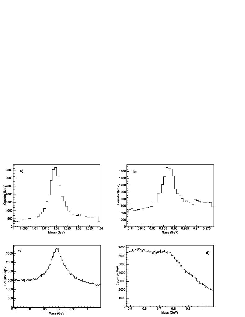
Figure 23: Invariant-mass distributions for the intermediate states involved in $D_{s}$ reconstruction. The plots are for 4160 MeV MC: a$)$ $\phi\rightarrow{K^{+}{K^{-}}}$, b$)$ $\eta^{{}^{\prime}}\rightarrow{\pi^{+}{\pi^{-}}\eta}$, c$)$ $K^{*}\rightarrow{K^{-}{\pi^{+}}}$, and d$)$ $\rho^{+}\rightarrow{\pi^{+}{\pi^{0}}}$.

8 Event Selection and Kinematics

We begin by assuming that charm production in the threshold region is dominated by final states with two charmed mesons and no other particles: $e^{+}e^{-}\rightarrow{D_{(s)}^{(*)}\bar{D}_{(s)}^{(*)}}$. For these events, the energy and momentum of the primary charmed mesons are well defined. In general, for $e^{+}e^{-}\rightarrow{X}{Y}$ in the center-of-mass frame we have

$$E_{X}=\frac{s+M_{X}^{2}-M_{Y}^{2}}{2\sqrt{s}}$$ (13)

and

$$|\vec{P_{X}}|=|\vec{P_{Y}}|=|\vec{P}|=\sqrt{E_{X}^{2}-M_{X}^{2}},$$ (14)

where $s=4E_{\rm{beam}}^{2}$. The energy and momentum of one of the two charmed mesons is therefore sufficient to assign an event to one of the possible two-body processes. In practice, we use familiar forms of these variables for this classification: the candidate’s beam-constrained mass ($M_{\rm{bc}}\equiv\sqrt{E_{\rm beam}^{2}-|\vec{P}|^{2}}~{}$) and its energy deficit relative to the beam ($\Delta E\equiv E_{\rm{beam}}-E_{D}$).

As the center-of-mass energy increases above $D\bar{D}$ and $D_{s}^{+}{D}_{s}^{-}$ thresholds, it becomes possible to produce the “starred” states, $D^{*0}$, $D^{*+}$ and $D_{s}^{*+}$. These are not fully reconstructed in this analysis, since momenta and energies are sufficient to identify the origin of the reconstructed $D_{(s)}$. Reconstructed $D$ and $D_{s}$ candidates from these sources do not have a well-defined momentum, since they are daughters of starred parents and exhibit Doppler broadening. This Doppler broadening manifests itself through smeared distributions in both energy and momentum. Some properties of the intermediate starred states are summarized in Table 11.

Table 11: $D^{*0}$, $D^{*+}$, and $D_{s}^{*+}$ decay modes [2]

Modes	Branching Fraction
$D^{*0}$ decays mode
$D^{0}\pi^{0}$	$61.9\pm 2.9\%$
$D^{0}\gamma$	$38.1\pm 2.9\%$
$D^{*+}$ decays mode
$D^{0}\pi^{+}$	$67.7\pm 0.5\%$
$D^{+}\pi^{0}$	$30.7\pm 0.5\%$
$D^{+}\gamma$	$1.6\pm 0.4\%$
$D_{s}^{*+}$ decays mode
$D_{s}^{+}\gamma$	$94.2\pm 2.5\%$
$D_{s}^{+}\pi^{0}$	$5.8\pm 2.5\%$

To illustrate the separation of events we show the momentum spectrum of $D^{0}$ candidates within 15 MeV of the nominal mass in Fig. 24 for the center-of-mass energy 4160 MeV. The top plot in Fig. 24 is from the MC described in Sect. 6 and the bottom plot is from the 10.16 pb^-1 of data. There are three distinct concentrations of entries near 0.95, 0.73 and 0.5 GeV/$c$, corresponding to $D\bar{D}$, $D^{*}\bar{D}$, and $D^{*}\bar{D}^{*}$ production, respectively. Similar distributions for $D_{s}$ candidates are shown in Fig. 25. In this case there are two distinct peaks in the MC at 0.675 and 0.4 GeV/$c$, corresponding to $D_{s}^{+}{D_{s}^{-}}$ and $D_{s}^{*+}{D_{s}^{-}}$, respectively, which are the only two accessible final states at this energy. Only the peak at 0.4 GeV/$c$ is visible in data, demonstrating that the cross section for $D_{s}^{+}{D_{s}^{-}}$ at this energy is consistent with zero. At center-of-mass energies above $D_{s}^{*+}D_{s}^{*-}$ threshold, such as 4260 MeV (not shown), there are three accessible final states, so three peaks in momentum are possible.

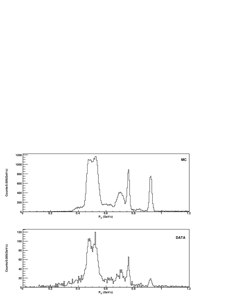
Figure 24: The momentum spectrum at 4160 MeV for $D^{0}\rightarrow{K^{-}}{\pi^{+}}$ candidates within 15 MeV of the nominal mass. The top plot is from the MC described in the text and the bottom plot is from the $10.16$ pb^-1 of data at this energy. The three distinct concentrations of entries near 0.95, 0.73 and 0.5 GeV/$c$ correspond to $D\bar{D}$, $D^{*}\bar{D}$, and $D^{*}\bar{D}^{*}$ production, respectively.

Figure 25: The momentum spectrum at 4160 MeV for $D_{s}^{+}\rightarrow{\phi}{\pi^{+}}$ candidates within 15 MeV of the nominal mass. The top plot is from the generic MC discussed in the text and the bottom plot is from the $10.16$ pb^-1 of data at this energy. The peak at $\sim 0.675$ MeV/$c$ is missing from the data, giving advanced notice that the cross section for ${D_{s}^{+}}{D_{s}^{-}}$ at this energy is consistent with zero.

For this analysis we need to separate clearly and measure the cross sections for the nine event types: $D^{0}\bar{D}^{0}$, $D^{*0}\bar{D}^{0}$, $D^{*0}\bar{D}^{*0}$, $D^{+}{D}^{-}$, $D^{*+}{D}^{-}$, $D^{*+}{D}^{*-}$, $D_{s}^{+}{D}_{s}^{-}$, $D_{s}^{*+}{D}_{s}^{-}$, and $D_{s}^{*+}{D}_{s}^{*-}$. We want to choose variables that are as orthogonal as possible for the purpose of this separation. For $D^{0}\bar{D}^{0}$, $D^{+}D^{-}$ and $D_{s}^{+}D_{s}^{-}$, the variables used were the $D$ candidate’s energy ($\Delta E$) and its momentum (in the form of $M_{\rm{bc}}$). The separation of $D$-meson candidates at 4160 MeV into the possible event types is illustrated in the $\Delta E$ vs. $M_{\rm{bc}}$ plot in Fig. 26. The corresponding plot for $D_{s}$ is given in Fig. 27. The quantitative task is to count the events and determine the cross section for each event category while controlling contributions from backgrounds and cross-feed from other two-charm final states.

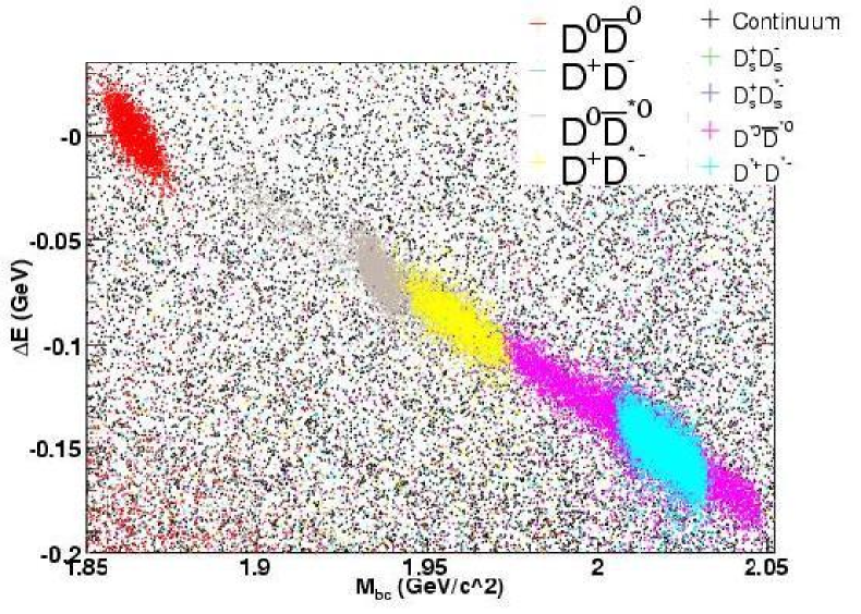
Figure 26: $\Delta E$ vs. $M_{\rm{bc}}$ for $D^{0}\rightarrow{K^{-}\pi^{+}}$ at 4160 MeV using the 100 pb^-1 MC sample. The plot illustrates the clear separation that is achieved for this choice of variables.

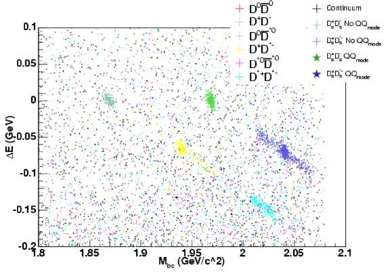
Figure 27: $\Delta E$ vs. $M_{\rm{bc}}$ for $D_{s}^{+}\rightarrow{\phi}{\pi^{+}}$ at 4160 MeV using the 100 pb^-1 MC sample. The plot illustrates the clear separation that is achieved by the choice of variables not just for $D_{s}$ but also for $D^{+}$ since the branching ratio for $D^{+}\rightarrow{\phi}{\pi^{+}}$ is nonzero.

To obtain the number of signal candidates for each event type, a signal region must first be defined. The signal region in $M_{\rm{bc}}$ for $D^{0}\bar{D}^{0}$, $D^{+}D^{-}$ and $D_{s}^{+}D_{s}^{-}$ is $\pm 9$ MeV around the respective particle masses. For the other event types ($D^{*0}\bar{D}^{0}$, $D^{*0}\bar{D}^{*0}$, $D^{*+}{D}^{-}$, $D^{*+}{D}^{*-}$, $D_{s}^{*+}{D}_{s}^{-}$, and $D_{s}^{*+}{D}_{s}^{*-}$) the requirement is $\pm 15$ MeV in invariant mass. To estimate combinatoric and other backgrounds, a sideband is defined on either side of the signal region. In every case the sidebands are spaced from the nominal particle mass by 5 $\sigma$. The sizes vary from mode to mode because of differing resolutions and the need to exclude potential peaking contributions (such as decay modes that are common between $D^{+}$ and $D_{s}^{+}$). These sidebands are all chosen to be significantly larger than the signal region to minimize the statistical uncertainty of the background subtraction. MC is used to determine the sideband normalization, which is defined as the total sideband yield divided by the MC-tagged background contribution in the signal region. In almost all cases the normalization given by MC is consistent with the ratio of the sizes of the signal and sideband regions. The background procedure is illustrated with one example for $M_{\rm{bc}}$ ($D^{+}\rightarrow K^{-}\pi^{+}\pi^{+}$ in $D^{+}D^{-}$) and one for invariant mass ($D^{+}\rightarrow K^{-}\pi^{+}\pi^{+}$ in $D^{*+}D^{*-}$) in Figs. 28 and 29, respectively.

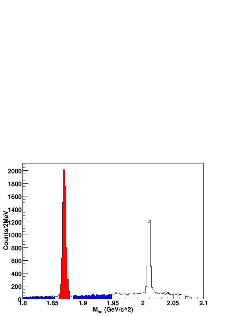
Figure 28: Plot of $M_{\rm{bc}}$ for $D^{+}\rightarrow{K^{-}\pi^{+}\pi^{+}}$ in $D^{+}D^{-}$ events in MC at 4160 MeV. The red indicates the signal region and the blue the sideband.

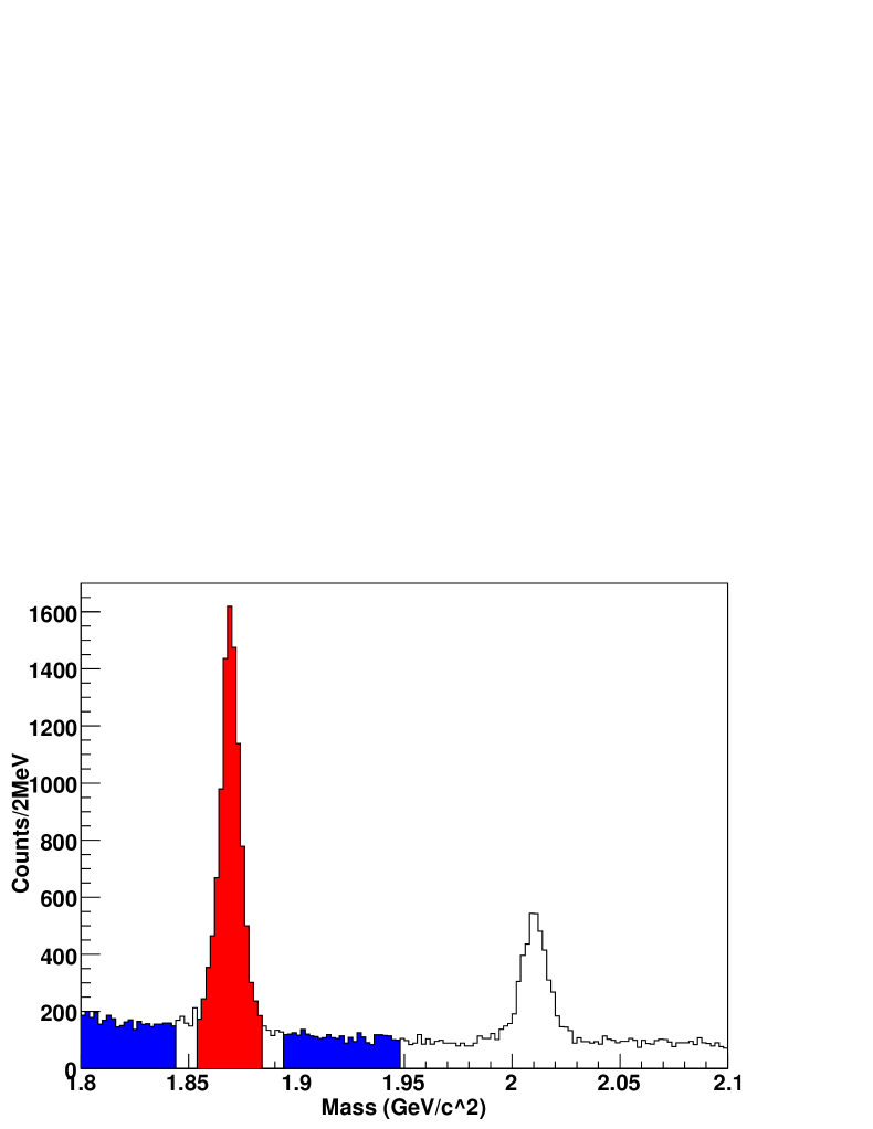
Figure 29: Plot of the invariant mass for $D^{+}\rightarrow K^{-}\pi^{+}\pi^{+}$ in $D^{*+}D^{*-}$ events in MC at 4160 MeV. The red indicates the signal region and the blue the sideband.

For the other event types (i.e. those involving one or two “starred” charmed mesons) the variables used for the separation were $M_{\rm{bc}}$ (candidate momentum) and invariant mass, which is a combination of momentum and energy. Regardless of the origin of a $D$ candidate, the invariant mass peaks at the $D$ mass. Since invariant mass does not differentiate between event types, $M_{\rm{bc}}$ provides all of the event-type separation for these events. The separation can be seen in Figs. 30 and 31.

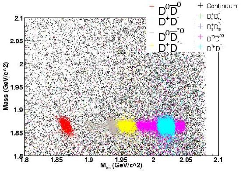
Figure 30: Invariant mass vs. $M_{\rm{bc}}$ for $D^{0}\rightarrow{K^{-}\pi^{+}}$ at 4160 MeV using the 100 pb^-1 MC sample. The plot illustrates the clear separation that is achieved with this choice of variables.

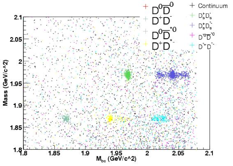
Figure 31: Invariant mass vs. $M_{\rm{bc}}$ for $D_{s}^{+}\rightarrow{\phi}{\pi^{+}}$ at 4160 MeV using the 100 pb^-1 MC sample. The plot illustrates the clear separation that is achieved with this choice of variables, not just for $D_{s}$ but also for $D^{+}$, since the branching ratio for $D^{+}\rightarrow{\phi}{\pi^{+}}$ is nonzero.

The difference in variable choices between unstarred and starred events is a matter of convenience. We use the same procedure that has been used with great success in the CLEO-c analysis of $\psi(3770)\rightarrow{D\bar{D}}$ in Refs. [45, 46]. $M_{\rm{bc}}$ has a practical advantage over the raw momentum in that $M_{\rm{bc}}$ changes much more slowly with beam energy. For a given center-of-mass energy, the expected values of $M_{\rm{bc}}$ and $\Delta E$ in $e^{+}e^{-}\rightarrow{X}{Y}$ are given by

$$M_{\rm{bc}}=\sqrt{\frac{1}{2}(M_{X}^{2}+M_{Y}^{2}-\frac{(M_{X}^{2}-M_{Y}^{2})^{2}}{2s})},$$ (15)

and

$$\Delta{E}=-\frac{1}{2}\frac{M_{X}^{2}-M_{Y}^{2}}{\sqrt{s}}.$$ (16)

As the center-of-mass energy increases from 3970 to 4180 MeV, $M_{\rm{bc}}$ for the $D$ in $D\bar{D}^{*}$ changes by $\sim 0.01\%$, while the momentum changes by $\sim 80\%$.

As discussed above, the method for $D^{0}\bar{D}^{0}$, $D^{+}D^{-}$ and $D_{s}^{+}D_{s}^{-}$ is to cut on $\Delta E$ ($\Delta E<15$ MeV) and use the $M_{\rm{bc}}$ distribution to determine the yield (Fig. 28). For all other event types the method is to cut on $M_{\rm{bc}}$ and use the invariant-mass distribution to determine the yield (Fig. 29). The cut on $M_{\rm{bc}}$ was determined by kinematics, since $M_{\rm{bc}}$ is center-of-mass energy dependent in addition to being dependent on the nature of the decay of the starred state. In order to choose the cut range we assumed that $D^{*0}$ and $D_{s}^{*+}$ decay $100\%$ of the time by $D^{*0}\rightarrow\gamma{D^{0}}$ and $D_{s}^{*+}\rightarrow\gamma{D_{s}^{+}}$, respectively, since the pion transitions will fall in the cut window for the $\gamma$ decay. We assumed that $D^{*+}$ decays only to $D^{+}\pi^{0}$ and $D^{0}\pi^{+}$, since the branching ratio for $D^{*+}\rightarrow{D^{+}}\gamma$ is only $1.6\%$. The equation that determines the $M_{\rm{bc}}$ cut window for $D^{*}\bar{D}$ and $D^{*}\bar{D}^{*}$ with $D^{*}\rightarrow{D}{X}$ is

$$M_{\rm{bc}}^{\rm{Lab}}=\sqrt{E_{\rm{beam}}^{2}-M_{D}^{2}-(\gamma{E_{D}}\pm\beta\gamma{P_{D}})^{2}},$$ (17)

with $\gamma=\frac{E_{D^{*}}}{M_{D^{*}}}$, $\beta\gamma=\frac{P_{D^{*}}}{M_{D^{*}}}$ and $E_{D}=\frac{M_{D^{*}}^{2}+M_{X}^{2}-M_{D}^{2}}{2M_{D^{*}}}$, where $M_{D},E_{D}$ and ${P_{D}}$ are the mass, energy, and momentum of the daughter $D$ in the rest frame of the $D^{*}$, and $E_{D^{*}}$ and $P_{D^{*}}$ are determined by Eqs. 13 and 14, respectively. For $D^{*0}$ and $D_{s}^{*+}$, $M_{X}=M_{\gamma}=0$, since only the $\gamma$ decay is considered in the calculation and for $D^{*+}$, $M_{X}=M_{\pi^{0}}=135$ MeV. After calculating the maximum and minimum values using the above equation and assumptions, we expand the interval by 5 MeV on each end to account for resolution effects.

An important point is that there is a certain energy at which an overlap between the $D^{0}\bar{D}^{*0}$ and $D^{*0}\bar{D}^{*0}$ will occur. This is only a problem for $D^{0}\bar{D}^{*0}$ and $D^{*0}\bar{D}^{*0}$, and not $D^{-}D^{*+}$ and $D^{*+}D^{*-}$, because only the ${\pi}$ decay was considered. This means these event types will have a significantly smaller cut window in $M_{\rm{bc}}$ as compared to neutral $D$ events. If this occurs, the high $M_{\rm{bc}}$ cut of $D^{0}\bar{D}^{*0}$ will be set equal to the low $M_{\rm{bc}}$ cut of $D^{*0}\bar{D}^{*0}$ so that events cannot pass both event-type cuts and be double-counted. This is done because $D^{*0}\bar{D}^{*0}$ will have twice as many $D$ mesons populating this area, assuming equal rates, therefore there will be less contamination from $D^{0}\bar{D}^{*0}$ in $D^{*0}\bar{D}^{*0}$ by this method as compared to its inverse.

Table 12: Selection criteria, in units of ${\rm{M_{bc}}}$, for measuring the cross sections for $D^{*}\bar{D}$ and $D^{*}\bar{D}^{*}$. A 15 MeV cut on $\Delta E$ was made when selecting $D\bar{D}$.

$E_{\rm{cm}}$ (MeV)	$D^{0}\bar{D}^{*0}$ ($\frac{\rm{GeV}}{c^{2}}$)	$D^{*0}\bar{D}^{*0}$ ($\frac{\rm{GeV}}{c^{2}}$)	$D^{+}{D}^{*-}$ ($\frac{\rm{GeV}}{c^{2}}$)	$D^{*+}{D}^{*-}$ ($\frac{\rm{GeV}}{c^{2}}$)
3970	$(1.902,1.972)$	$-$	$(1.933,1.958)$	$-$
3990	$(1.901,1.976)$	$-$	$(1.933,1.961)$	$-$
4010	$(1.899,1.98)$	$-$	$(1.934,1.963)$	$-$
4015	$(1.899,1.981)$	$(1.994,2.01)$	$(1.934,1.963)$	$-$
4030	$(1.898,1.984)$	$(1.987,2.02)$	$(1.934,1.965)$	$(2.003,2.018)$
4060	$(1.896,1.98)$	$(1.98,2.03)$	$(1.935,1.968)$	$(2.002,2.022)$
4120	$(1.893,1.974)$	$(1.974,2.044)$	$(1.935,1.974)$	$(2.003,2.029)$
4140	$(1.892,1.972)$	$(1.972,2.048)$	$(1.935,1.976)$	$(2.004,2.032)$
4160	$(1.891,1.97)$	$(1.97,2.052)$	$(1.935,1.978)$	$(2.004,2.034)$
4170	$(1.89,1.97)$	$(1.97,2.054)$	$(1.935,1.979)$	$(2.005,2.035)$
4180	$(1.89,1.969)$	$(1.969,2.056)$	$(1.935,1.98)$	$(2.005,2.036)$
4200	$(1.889,1.968)$	$(1.968,2.06)$	$(1.935,1.982)$	$(2.006,2.038)$
4260	$(1.887,1.965)$	$(1.965,2.071)$	$(1.935,1.988)$	$(2.008,2.044)$

Table 13: Selection criteria, in units of ${\rm{M_{bc}}}$, for measuring the cross section for $D_{s}^{*}\bar{D}_{s}$ and $D^{*}_{s}\bar{D}^{*}_{s}$. A 15 MeV cut on $\Delta E$ was made when selecting $D_{s}\bar{D}_{s}$.

Ecm MeV	$D^{+}_{s}{D}^{*-}_{s}~{}\frac{\rm{GeV}}{\rm{c^{2}}}$	$D^{*+}_{s}{D}^{*-}_{s}~{}\frac{\rm{GeV}}{\rm{c^{2}}}$
3970	$-$	$-$
3990	$-$	$-$
4010	$-$	$-$
4015	$-$	$-$
4030	$-$	$-$
4060	$-$	$-$
4120	$(2.015,2.06)$	$-$
4140	$(2.011,2.067)$	$-$
4160	$(2.009,2.071)$	$-$
4170	$(2.008,2.073)$	$-$
4180	$(2.007,2.076)$	$-$
4200	$(2.005,2.08)$	$-$
4260	$(2.001,2.087)$	$(2.087,2.132)$

Chapter Cross Section Calculation

9 Determination of Cross Sections

9.1 Exclusive Cross Sections

The cross section for $D_{(s)}$ from any of the nine possible event types can be computed with the following equation:

$$\sigma_{D_{(s)}^{(*)}\bar{D}_{(s)}^{(*)}}(D_{(s)})=\frac{N(\rm{signal})}{{\cal{B}}{\cal{L}}\epsilon},$$ (18)

where $N(\rm{signal})$ is the number of signal events, ${\cal{B}}$ is the branching ratio for the particular $D$ decay being used (Table 9 [2, 44] and Table 10 [45, 46]), $\cal{L}$ is the integrated luminosity, and $\epsilon$ is the detection efficiency (determined with MC).

$N(\rm{signal})$ is obtained by counting candidates in the signal region and subtracting sideband-estimated backgrounds with normalizations determined by MC. This procedure and the definitions of the signal and sideband regions for each mode appear in Sect. 8.

The cross sections for the $D\bar{D}$, $D^{*}\bar{D}$ and $D^{*}\bar{D}^{*}$ production modes are calculated as follows:

$$\sigma(D^{*+}D^{*-})=\frac{\sigma_{D^{*}\bar{D}^{*}}(D^{+})}{2(1-{\cal{B}}(D^{*+}\rightarrow{D^{0}\pi^{+}}))},$$ (19)

$$\sigma(D^{*0}\bar{D}^{*0})=\frac{1}{2}(\sigma_{D^{*}\bar{D}^{*}}(D^{0})-2{\cal{B}}(D^{*+}\rightarrow{D^{0}\pi^{+}})\sigma(D^{*+}D^{*-})),$$ (20)

$$\sigma(D^{*+}D^{-})=\frac{\sigma_{D^{*}\bar{D}}(D^{+})}{2-{\cal{B}}(D^{*+}\rightarrow{D^{0}\pi^{+}})},$$ (21)

$$\sigma(D^{*0}\bar{D}^{0})=\frac{1}{2}(\sigma_{D^{*}\bar{D}}(D^{0})-{\cal{B}}(D^{*+}\rightarrow{D^{0}\pi^{+}})\sigma(D^{*+}D^{-})),$$ (22)

$$\sigma(D^{+}D^{-})=\frac{\sigma_{D\bar{D}}(D^{+})}{2},$$ (23)

and

$$\sigma(D\bar{D})=\frac{\sigma_{D\bar{D}}(D^{0})}{2},$$ (24)

where $\sigma_{D^{*}\bar{D}^{*}}(D^{+})$ is the cross section of $D^{+}$ produced in $D^{*}\bar{D}^{*}$ events, $\sigma_{D^{*}\bar{D}^{*}}(D^{0})$ is the cross section of $D^{0}$ produced in $D^{*}\bar{D}^{*}$ events, $\sigma_{D^{*}\bar{D}}(D^{+})$ is the cross section of $D^{+}$ produced in $D^{*}\bar{D}$ events, $\sigma_{D^{*}\bar{D}}(D^{0})$ is the cross section of $D^{0}$ produced in $D^{*}\bar{D}$ events, $\sigma_{D\bar{D}}(D^{+})$ is the cross section of $D^{+}$ produced in $D\bar{D}$ events, and $\sigma_{D\bar{D}}(D^{0})$ is the cross section of $D^{0}$ produced in $D\bar{D}$ events.

To determine $\sigma(D^{0})$ and $\sigma(D^{+})$, weighted averages of the three $D^{0}$ modes and five $D^{+}$ modes are calculated, with weights defined as $\frac{1}{\sigma_{\sigma(D)_{i}}^{2}}$.

For $D_{s}\bar{D}_{s}$, $D_{s}^{*}\bar{D}_{s}$ and $D_{s}^{*}\bar{D}_{s}^{*}$, a weighted sum technique is used to combine the eight $D_{s}$ decay modes and obtain the cross sections. The weights that minimize the error are given by the following:

$$w_{i}=\frac{\frac{1}{f_{i}^{2}N_{i}}}{\sum_{i=0}^{8}\frac{1}{f_{i}^{2}N_{i}}},$$ (25)

where $f_{i}=\frac{\sigma_{i}}{N_{i}}$, $N_{i}$ is the yield, $\sigma_{i}$ is the uncertainty on the yield for mode $i$. It is perhaps counterintuitive that for modes with equal precision the weight is inversely proportional to the yield, thereby suppressing the weight of modes with high yields. This feature guarantees that the weighting of different modes in the cross section measurement is determined by the precision of the yield measurement rather than its magnitude. (The conclusion can be easily verified by considering a “toy” example of two modes, each with 10% precision and yields of 100 and 1000, respectively. Eq. 25 properly assigns roughly equal weighting and achieves an uncertainty of $\sim 7\%$, rather than the 10% that would follow if the “bigger” mode were allowed to dominate.)

The weights were determined by MC for each of the eight modes for each of the three possible event types, $D_{s}\bar{D}_{s}$, $D_{s}^{*}\bar{D}_{s}$, $D_{s}^{*}\bar{D}_{s}^{*}$. The weights were then averaged across these possible event types and used in calculating the cross sections. The equation for determining either the $D_{s}\bar{D}_{s}$, $D_{s}^{*}\bar{D}_{s}$, $D_{s}^{*}\bar{D}_{s}^{*}$ cross sections is as follows:

$$\sigma(D_{s}^{(*)+}D_{s}^{(*)-})=\frac{(\sum^{8}_{i=1}N_{i}^{DATA}w_{i})}{\epsilon{\cal{L}}},$$ (26)

where $\epsilon$ is determined with MC by the following:

$$\epsilon=\frac{(\sum_{i=1}^{8}N^{MC}_{i}w_{i})}{N_{generated}},$$ (27)

where the $8$ in the summation refers to the eight $D_{s}$ modes that were used during the scan.

9.2 Efficiencies for Exclusive Selection

Efficiencies for exclusive selection of all accessible event types and center-of-mass energies were determined by analyzing the MC samples described in Sect. 6. The efficiency for detecting a particular decay mode is defined as follows:

$$\epsilon=\frac{N^{\rm{MC}}_{\rm{detected}}}{N^{\rm{MC}}_{\rm{generated}}},$$ (28)

where the error is determined by binomial statistics:

$$\sigma_{\epsilon}=\sqrt{\frac{\epsilon(1-\epsilon)}{N^{\rm{MC}}_{\rm{generated}}}}.$$ (29)

$N^{\rm{MC}}_{\rm{detected}}$ is obtained by applying the same selection and background-correction procedures to MC as are used to determine the signal yields in data. The efficiencies for each of the twelve energies and event types are listed in Tables 14 ($D^{0}$), 15 ($D^{+}$) and 48 ($D_{s}^{+}$ - note that this multi-page table appears on P.193 after the References).

Table 14: Efficiencies (units of $10^{-2}$) at each scan-energy point for selection of $D^{0}\rightarrow{K^{-}}\pi^{+}$ decays in the three exclusive event types.

Ecm (MeV)	$D\bar{D}$	$D^{*}\bar{D}$	$D^{*}\bar{D}^{*}$
$3970$	$62.42\pm 0.72$	$61.78\pm 0.36$	$-\pm-$
$3990$	$63.04\pm 0.72$	$62.37\pm 0.36$	$-\pm-$
$4010$	$61.75\pm 0.73$	$62.83\pm 0.36$	$-\pm-$
$4015$	$62.29\pm 0.59$	$63.31\pm 0.36$	$64.23\pm 0.24$
$4030$	$63.75\pm 0.63$	$62.68\pm 0.39$	$64.60\pm 0.24$
$4060$	$60.17\pm 0.64$	$61.24\pm 0.39$	$64.42\pm 0.24$
$4120$	$58.97\pm 0.66$	$59.75\pm 0.40$	$64.23\pm 0.25$
$4140$	$59.49\pm 0.47$	$57.90\pm 0.29$	$64.84\pm 0.17$
$4160$	$57.94\pm 0.66$	$58.12\pm 0.40$	$64.80\pm 0.25$
$4170$	$58.12\pm 0.66$	$56.53\pm 0.40$	$65.23\pm 0.25$
$4180$	$59.30\pm 0.66$	$54.72\pm 0.41$	$66.00\pm 0.25$
$4200$	$59.06\pm 0.66$	$52.52\pm 0.41$	$66.88\pm 0.24$
$4260$	$56.29\pm 1.01$	$41.36\pm 0.61$	$70.02\pm 0.36$

Table 15: Efficiencies (units of $10^{-2}$) at each scan-energy point for selection of $D^{+}\rightarrow{K^{-}}\pi^{+}\pi^{+}$ decays in the three exclusive event types.

Ecm MeV	$D\bar{D}$	$D^{*}\bar{D}$	$D^{*}\bar{D}^{*}$
$3970$	$56.07\pm 0.49$	$52.82\pm 0.35$	$-\pm-$
$3990$	$55.33\pm 0.48$	$52.78\pm 0.35$	$-\pm-$
$4010$	$55.59\pm 0.49$	$53.13\pm 0.35$	$-\pm-$
$4015$	$53.60\pm 0.39$	$53.37\pm 0.34$	$-\pm-$
$4030$	$56.79\pm 0.43$	$52.33\pm 0.37$	$53.60\pm 0.38$
$4060$	$53.93\pm 0.43$	$52.53\pm 0.37$	$53.12\pm 0.38$
$4120$	$54.42\pm 0.44$	$52.55\pm 0.38$	$51.64\pm 0.38$
$4140$	$53.83\pm 0.31$	$51.18\pm 0.27$	$52.47\pm 0.27$
$4160$	$54.12\pm 0.44$	$51.10\pm 0.38$	$50.98\pm 0.38$
$4170$	$54.15\pm 0.44$	$51.15\pm 0.38$	$51.31\pm 0.38$
$4180$	$54.25\pm 0.44$	$51.39\pm 0.38$	$52.46\pm 0.38$
$4200$	$53.38\pm 0.44$	$51.37\pm 0.38$	$52.47\pm 0.38$
$4260$	$54.51\pm 0.66$	$49.15\pm 0.58$	$51.29\pm 0.59$

9.3 Cross Section Results

Following the procedure laid out in the previous sections, the production cross sections were measured at thirteen center-of-mass energies. The results are shown in Tables 51 and 52 and Figs. 32 and 33.

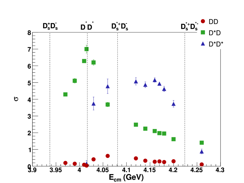
Figure 32: Observed cross sections for $e^{+}e^{-}\rightarrow{D\bar{D}}$, $D^{*}\bar{D}$ and $D^{*}\bar{D}^{*}$ as a function of center-of-mass energy. Errors are just statistical.

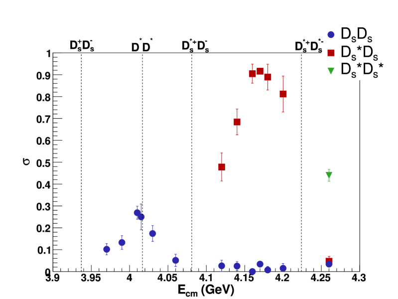
Figure 33: Observed cross sections for $e^{+}e^{-}\rightarrow{D_{s}\bar{D}_{s}}$, $D_{s}^{*}\bar{D}_{s}$ and $D_{s}^{*}\bar{D}_{s}^{*}$ as a function of center-of-mass energy from the scan. Errors are just statistical.

These cross sections were then used in Eqs. 19-24 to obtain the results shown in Tables 51 and 52.

The weights and efficiencies are shown in Tables 16 and 17. By summing the individual exclusive cross sections, one arrives at the total observed charm cross section which is shown, along with the exclusive cross sections, in Table 51 and 52.

Table 16: The efficiencies in units of $10^{-2}$ for detecting $D_{s}\bar{D}_{s}$, $D_{s}^{*}\bar{D}_{s}$, and $D_{s}^{*}\bar{D}_{s}^{*}$ at each energy point in the CLEO-c scan.

Ecm MeV	$\epsilon({D_{s}^{+}D_{s}^{-}})$	$\epsilon(D_{s}^{*+}{D_{s}^{-}})$	$\epsilon({D^{*+}_{s}D^{*-}_{s}})$
$3970$	$1.14\pm 0.02$	$-\pm-$	$-\pm-$
$3990$	$1.11\pm 0.02$	$-\pm-$	$-\pm-$
$4010$	$1.11\pm 0.02$	$-\pm-$	$-\pm-$
$4015$	$1.13\pm 0.02$	$-\pm-$	$-\pm-$
$4030$	$1.20\pm 0.02$	$-\pm-$	$-\pm-$
$4060$	$1.09\pm 0.02$	$-\pm-$	$-\pm-$
$4100$	$1.12\pm 0.03$	$1.00\pm 0.02$	$-\pm-$
$4120$	$1.04\pm 0.03$	$1.04\pm 0.02$	$-\pm-$
$4140$	$1.04\pm 0.02$	$1.06\pm 0.02$	$-\pm-$
$4160$	$1.09\pm 0.03$	$1.06\pm 0.02$	$-\pm-$
$4170$	$1.09\pm 0.03$	$1.06\pm 0.02$	$-\pm-$
$4180$	$1.09\pm 0.03$	$1.10\pm 0.03$	$-\pm-$
$4200$	$1.09\pm 0.03$	$1.07\pm 0.03$	$-\pm-$
$4260$	$1.09\pm 0.03$	$1.10\pm 0.03$	$1.05\pm 0.03$

Table 17: For $D_{s}\bar{D}_{s}$, $D_{s}^{*}\bar{D}_{s}$, and $D_{s}^{*}\bar{D}_{s}^{*}$, a weighted sum technique that minimize the error is used to determine the cross sections. The weights for each mode are shown below. The mode with the largest weight is $\phi\pi^{+}$, which is by far the cleanest of all the modes.

Mode	Weight
$K_{s}K^{+}$	$0.14$
$\eta\pi^{+}$	$0.06$
$\phi\pi^{+}$	$0.23$
$K^{*}K^{+}$	$0.12$
$\eta\rho^{+}$	$0.05$
$\eta^{{}^{\prime}}\pi^{+}$	$0.16$
$\eta^{{}^{\prime}}\rho^{+}$	$0.10$
$\phi\rho^{+}$	$0.13$

9.4 Two Other Methods for Measuring the Total Charm Cross Section

9.4.1 Inclusive $D$ Method

In addition to measuring the separate cross sections for all expected charm event types, one can perform inclusive measurements to obtain the total observed charm cross section.

As for the exclusive measurements, the efficiencies for inclusively selecting events with charmed mesons are determined with the MC samples described in Sect. 6. They are given in Table 18.

Table 18: Efficiencies at each scan-energy point for inclusive selection of $D^{0}\rightarrow{K^{-}}\pi^{+}$, $D^{+}\rightarrow{K^{-}}\pi^{+}\pi^{+}$, and $D_{s}^{+}\rightarrow{K^{-}}K^{+}\pi^{+}$ (units of $10^{-2}$).

Ecm MeV	$\epsilon(D^{0}\rightarrow{K^{-}}\pi^{+})$	$\epsilon(D^{+}\rightarrow{K^{-}}\pi^{+}\pi^{+})$	$\epsilon(D_{s}^{+}\rightarrow{K^{-}}K^{+}\pi^{+})$
$3970$	$63.26\pm 0.32$	$53.07\pm 0.28$	$54.31\pm 0.90$
$3990$	$61.99\pm 0.33$	$52.29\pm 0.28$	$53.04\pm 0.90$
$4010$	$62.52\pm 0.32$	$53.57\pm 0.28$	$53.62\pm 0.90$
$4015$	$63.79\pm 0.19$	$51.91\pm 0.26$	$52.10\pm 0.74$
$4030$	$64.52\pm 0.20$	$53.47\pm 0.23$	$52.87\pm 0.81$
$4060$	$63.24\pm 0.20$	$51.95\pm 0.23$	$48.83\pm 0.80$
$4120$	$62.49\pm 0.20$	$52.33\pm 0.23$	$50.90\pm 0.59$
$4140$	$62.61\pm 0.14$	$51.79\pm 0.16$	$49.84\pm 0.42$
$4160$	$62.54\pm 0.20$	$51.17\pm 0.23$	$52.75\pm 0.59$
$4170$	$62.26\pm 0.20$	$51.39\pm 0.23$	$52.93\pm 0.59$
$4180$	$62.32\pm 0.20$	$51.95\pm 0.23$	$53.67\pm 0.59$
$4200$	$63.13\pm 0.20$	$52.00\pm 0.23$	$51.63\pm 0.59$
$4260$	$60.82\pm 0.31$	$51.35\pm 0.35$	$53.74\pm 0.69$

For $D^{0}$ and $D^{+}$, the event-type requirements on $|\Delta E|$ and $M_{\rm{bc}}$ are lifted and the invariant mass is used to extract the yields. The inclusive $D^{0}\rightarrow{K^{-}\pi^{+}}$ and $D^{+}\rightarrow{K^{-}\pi^{+}\pi^{+}}$ invariant-mass spectra are shown for the 4160 MeV data sample in Figs. 34 and 35. For $D_{s}$ the event-type requirements are preserved because of the need to suppress the background for the high-yield mode $K^{-}K^{+}\pi^{+}$. At energies above $4100$ MeV, for all candidates that pass the selection requirements for $D_{s}^{+}D_{s}^{-}$, $D_{s}^{*+}D_{s}^{-}$ and $D_{s}^{*+}D_{s}^{*-}$ (the last only for $4260$ MeV), the invariant mass is used to determine the inclusive yield. At energies below $4100$ MeV, $M_{\rm{bc}}$ is used to determine the yield since these energies are below $D_{s}^{*+}D_{s}^{-}$ and $D_{s}^{*+}D_{s}^{*-}$ thresholds. The inclusive $D_{s}^{+}\rightarrow{K^{-}K^{+}\pi^{+}}$ invariant mass in 4160 MeV data is shown in Fig. 36. Each histogram is fitted to a function that includes a Gaussian signal and an appropriate background function. For $D^{0}\rightarrow{K^{-}\pi^{+}}$, $D^{+}\rightarrow{K^{-}\pi^{+}\pi^{+}}$ and $D_{s}^{+}\rightarrow{K^{-}K^{+}\pi^{+}}$ above $4100$ MeV, the background function is a second-order polynomial. For $D_{s}^{+}\rightarrow{K^{-}K^{+}\pi^{+}}$ below $4100$ MeV, the background function is an Argus function [48]. The results of the fits are shown in Table 19.

Figure 34: The invariant mass of $D^{0}\rightarrow{K^{-}}{\pi^{+}}$ in data at $E_{cm}=4160$ MeV.

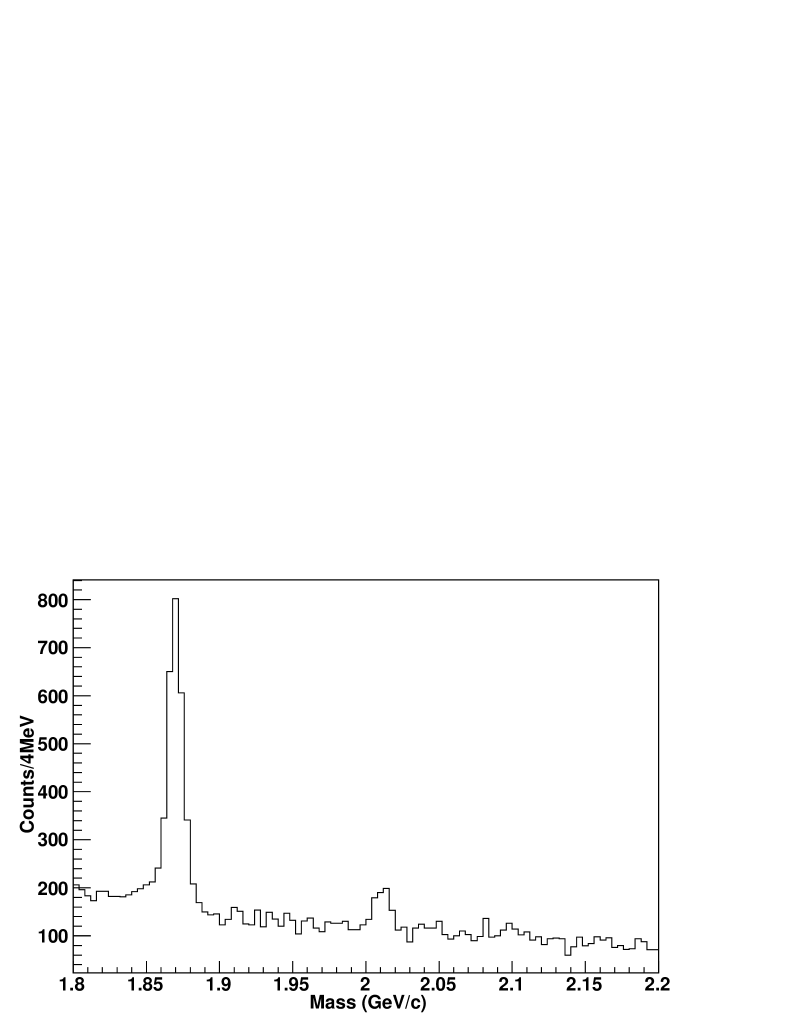
Figure 35: The invariant mass of $D^{+}\rightarrow{K^{-}}{\pi^{+}}{\pi^{+}}$ in data at $E_{cm}=4160$ MeV. The peak at $\sim 2$ GeV is fully reconstructed $D^{*+}\rightarrow{D^{0}\pi^{+}}$, $D^{0}\rightarrow{K^{-}\pi^{+}}$.

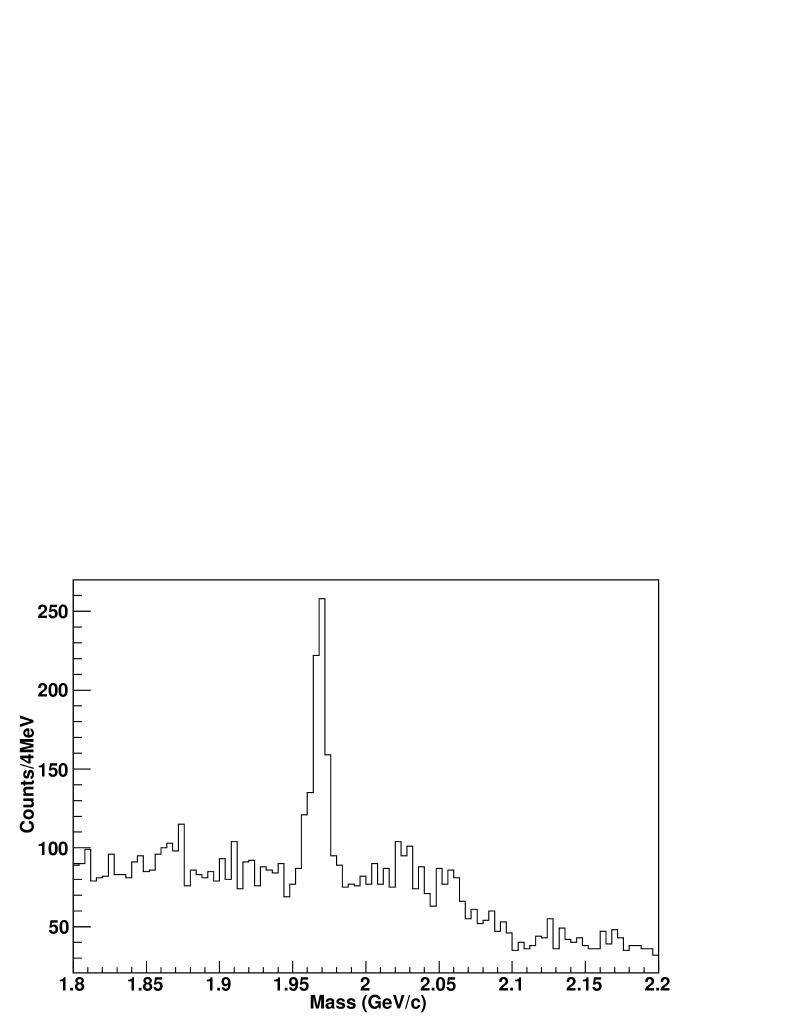
Figure 36: The invariant mass of $D_{s}^{+}\rightarrow{K^{+}}{K^{-}}{\pi^{+}}$ in data at $E_{cm}=4160$ MeV.

Table 19: Yields from inclusive fits for ${D^{0}}$, ${D^{+}}$ and ${D^{+}_{s}}$.

Ecm MeV	${(D^{0})}$	${(D^{+})}$	${(D^{+}_{s})}$
3970	$595.52\pm 28.25$	$636.42\pm 32.33$	$35.82\pm 14.47$
3990	$643.91\pm 29.35$	$600.57\pm 30.36$	$34.04\pm 7.50$
4010	$1280.07\pm 40.56$	$1256.24\pm 43.55$	$69.50\pm 11.70$
4015	$370.27\pm 21.35$	$346.65\pm 22.61$	$16.19\pm 5.58$
4030	$1192.53\pm 37.29$	$844.87\pm 36.18$	$43.42\pm 9.14$
4060	$1191.66\pm 37.68$	$859.62\pm 36.77$	$0.00\pm 0.00$
4120	$881.87\pm 32.89$	$576.56\pm 30.62$	$77.30\pm 14.50$
4140	$1512.51\pm 43.45$	$1006.17\pm 42.40$	$181.21\pm 21.29$
4160	$3130.11\pm 62.79$	$2028.33\pm 59.92$	$448.12\pm 32.75$
4170	$54958\pm 262.702$	$34050.8\pm 247.879$	$8379.97\pm 146.051$
4180	$1668.05\pm 46.10$	$1088.37\pm 44.12$	$243.47\pm 23.80$
4200	$727.11\pm 30.61$	$445.36\pm 27.59$	$97.80\pm 15.19$
4260	$1691.56\pm 51.13$	$1370.82\pm 52.60$	$330.49\pm 34.93$

The observed inclusive cross section can be determined as follows:

$$\sigma(e^{+}e^{-}\rightarrow{D_{(s)}}X)=\frac{N(\rm{signal})}{{\cal{B}}{\cal{L}}\epsilon},$$ (30)

where $N(\rm{signal})$ is the signal yield from the inclusive fit (Table 19), $\epsilon$ is the efficiency for detecting the signal (Table 18), ${\cal{B}}$ is the branching ratio for the particular $D$ decay in question, and $\cal{L}$ is the integrated luminosity. The cross section times branching ratio for $D^{0}$, $D^{+}$ and $D_{s}$ and the cross sections determined from these with the branching ratios in Ref. [45] and Ref. [2] are shown in Tables 20 and 21, respectively.

Table 20: The cross section, in nb, times branching ratio of ${D^{0}}$, ${D^{+}}$ and ${D^{+}_{s}}$.

Ecm	$\sigma\cdot{{\cal{B}}}(D^{0}\rightarrow{K^{-}\pi^{+}})$	$\sigma\cdot{{\cal{B}}}(D^{+}\rightarrow{K^{-}\pi^{+}\pi^{+}})$	$\sigma\cdot{{\cal{B}}}(D^{+}_{s}\rightarrow{K^{-}K^{+}\pi^{+}})$
3970	$0.244\pm 0.012$	$0.311\pm 0.016$	$0.017\pm 0.007$
3990	$0.309\pm 0.014$	$0.342\pm 0.017$	$0.019\pm 0.004$
4010	$0.364\pm 0.012$	$0.417\pm 0.014$	$0.023\pm 0.004$
4015	$0.395\pm 0.023$	$0.454\pm 0.030$	$0.021\pm 0.007$
4030	$0.615\pm 0.019$	$0.526\pm 0.023$	$0.027\pm 0.006$
4060	$0.574\pm 0.018$	$0.504\pm 0.022$	$0.000\pm 0.000$
4120	$0.511\pm 0.019$	$0.399\pm 0.021$	$0.055\pm 0.010$
4140	$0.496\pm 0.014$	$0.399\pm 0.017$	$0.075\pm 0.009$
4160	$0.493\pm 0.010$	$0.390\pm 0.012$	$0.084\pm 0.006$
4170	$0.493\pm 0.002$	$0.370\pm 0.003$	$0.088\pm 0.002$
4180	$0.472\pm 0.013$	$0.370\pm 0.015$	$0.080\pm 0.008$
4200	$0.410\pm 0.017$	$0.305\pm 0.019$	$0.067\pm 0.010$
4260	$0.212\pm 0.006$	$0.204\pm 0.008$	$0.048\pm 0.005$

Table 21: The inclusive cross section of ${D^{0}}$, ${D^{+}}$, and ${D^{+}_{s}}$

Ecm MeV	$\sigma_{(D^{0})}$ nb	$\sigma_{(D^{+})}$ nb	$\sigma_{(D^{+}_{s})}$ nb
3970	$6.25\pm 0.30$	$3.27\pm 0.17$	$0.31\pm 0.13$
3990	$7.92\pm 0.36$	$3.59\pm 0.18$	$0.34\pm 0.08$
4010	$9.31\pm 0.30$	$4.38\pm 0.15$	$0.41\pm 0.07$
4015	$10.10\pm 0.58$	$4.77\pm 0.31$	$0.38\pm 0.13$
4030	$15.73\pm 0.49$	$5.52\pm 0.24$	$0.49\pm 0.10$
4060	$14.67\pm 0.46$	$5.29\pm 0.23$	$-\pm-$
4120	$13.08\pm 0.49$	$4.19\pm 0.22$	$0.99\pm 0.19$
4140	$12.68\pm 0.36$	$4.19\pm 0.18$	$1.34\pm 0.16$
4160	$12.60\pm 0.25$	$4.10\pm 0.12$	$1.50\pm 0.11$
4170	$12.51\pm 0.06$	$3.90\pm 0.03$	$1.59\pm 0.03$
4180	$12.08\pm 0.33$	$3.88\pm 0.16$	$1.44\pm 0.14$
4200	$10.48\pm 0.44$	$3.20\pm 0.20$	$1.21\pm 0.19$
4260	$5.43\pm 0.16$	$2.14\pm 0.08$	$0.86\pm 0.09$

From the inclusive cross sections, the total charm cross section can be obtained. Since all $D$ mesons are produced in pairs the total cross section for production of charm events is given by

$$\sigma(e^{+}e^{-}\rightarrow{D\bar{D}}X)=\frac{\sigma_{D^{0}}+\sigma_{D^{+}}+\sigma_{D^{+}_{s}}}{2}$$ (31)

at each energy point. These results are given in Table 22.

Table 22: The total charm cross section as obtained by the inclusive method

Ecm MeV	$\sigma(e^{+}e^{-}\rightarrow{D\bar{D}X})$ nb
3970	$4.910\pm 0.183$
3990	$5.926\pm 0.219$
4010	$7.050\pm 0.180$
4015	$7.623\pm 0.360$
4030	$10.870\pm 0.294$
4060	$9.979\pm 0.258$
4120	$9.132\pm 0.281$
4140	$9.105\pm 0.212$
4160	$9.103\pm 0.147$
4170	$9.094\pm 0.066$
4180	$8.701\pm 0.193$
4200	$7.448\pm 0.250$
4260	$4.212\pm 0.093$

9.4.2 Hadron-Counting Method

Still another method and cross-check can be done. This method involves counting the multihadronic events in the data at all thirteen energy points and using data collected below $c{\bar{c}}$ threshold at $E_{\rm{cm}}=3671$ MeV to subtract $uds$ continuum production. Except for one difference to be discussed later, this method is the same as that used by CLEO-c [49, 50, 51] to determine the cross section of $e^{+}e^{-}\rightarrow\psi(3770)\rightarrow{hadrons}$ at $E_{\rm{cm}}=3770$ MeV. The Standard Hadron (SHAD) cuts as discussed in Refs. [49, 51] are used.

This method first starts by calculating the number of hadronic continuum events at $E_{\rm{cm}}=3671$ MeV:

$$N(3671)=(N_{{\rm{obs}}}-N_{\psi(2S)}-N_{J/\psi}\cdot\epsilon_{J/\psi}-N_{ee}\cdot\epsilon_{ee}-N_{\mu\mu}\cdot\epsilon_{\mu\mu}-N_{\tau\tau}\cdot\epsilon_{\tau\tau})/\epsilon_{{\rm{cont}}},$$ (32)

where the $N$’s are the numbers of events of different types as determined from data or by calculating ${\cal{L}}\cdot\sigma$, and the $\epsilon$’s are the efficiencies for passing the SHAD cuts of the same event types. The hadronic efficiency for events from the $uds$ continuum is $\epsilon_{cont}$. The quantity $N_{\psi(2S)}$ in Eq. 32 is the contribution due to the Breit-Wigner tail of $\psi(2S)$. It is estimated from the data collected at $E_{\rm{cm}}=3671$ and 3686 MeV as follows:

$$N(\psi(2S))_{3671}=\frac{N(\pi^{+}\pi^{-}l^{+}l^{-})_{3671}}{N(\pi^{+}\pi^{-}l^{+}l^{-})_{3686}}\cdot{N(\psi(2S))_{3686}},$$ (33)

where ${N(\psi(2S))_{3686}}$ is the number of hadronic events in $\psi(2S)$ decays at $E_{\rm{cm}}=3686$ MeV. The values used for $N(\pi^{+}\pi^{-}l^{+}l^{-})_{3686}$ and $N(\pi^{+}\pi^{-}l^{+}l^{-})_{3671}$ in Eq. 32 were obtained by CLEO-c [55] and give a scale factor of $\frac{N(\pi^{+}\pi^{-}l^{+}l^{-})_{3671}}{N(\pi^{+}\pi^{-}l^{+}l^{-})_{3686}}=\frac{221}{30462}=0.0073$. The number of hadronic events in $\psi(2S)$ decays at $E_{\rm{cm}}=3686$ MeV is determined by

$$N(\psi(2S))_{3686}=N(3868)_{\rm{obs}}-S\cdot{N_{{\rm{obs}}}(3671)},$$ (34)

where the scale factor, $S=\frac{{\cal{L}}_{3686}}{{\cal{L}}_{3671}}\cdot(\frac{3671}{3686})^{2}=0.139$. In Eq. 34 we neglect the contamination of $\psi(2S)$ in the off-resonance data and QED events, which is small compared to the large number of $\psi(2S)$ decays present in the sample.

After determining $N(3671)_{\rm{obs}}$, it can be used in determining the number of hadronic events at each scan point as follows:

$$N(X)=(N_{{\rm{obs}}}(X)-S\cdot{N_{{\rm{obs}}}(3671)}-N_{\psi(2S)}\cdot\epsilon_{\psi(2S)}-N_{\psi(3770)}\cdot\epsilon_{\psi(3770)}-$$

$$N_{J/\psi}\cdot\epsilon_{J/\psi}-N_{ee}\cdot\epsilon_{ee}-N_{\mu\mu}\cdot\epsilon_{\mu\mu}-N_{\tau\tau}\cdot\epsilon_{\tau\tau}),$$ (35)

where X stands for the energy point in question (3970, 3990, 4010, 4015, 4030, 4060, 4120, 4140, 4160, 4170, 4180, 4200, and 4260 MeV), and $S$ is the scale factor given by $\frac{{\cal{L}}_{X}}{{\cal{L}}_{3671}}\cdot(\frac{3671~{}{\rm{MeV}}}{X~{}{\rm{MeV}}})^{2}$.

In determining $N(3671)$ CLEO-c’s method was followed exactly; that is the data collected at the $\psi(2S)$ resonance was used in determining $N_{\psi(2S)}$ in Eq. 32. However, in regards to $N(X)$ we used the calculated production cross section in determining the amount of $\psi(2S)$, in addition to the amount of $J/\psi$ and $\psi(3770)$ present at each energy point. The calculated production cross section is a convolution of a $\delta$-function-approximated Breit-Wigner and an ISR kernel:

$$\sigma(e^{+}e^{-}\rightarrow\gamma{X})=\frac{12\pi^{2}\Gamma_{ee}}{s{\rm{M_{X}}}}\cdot f(s,x),$$ (36)

where the ISR kernel f(x,s) is defined in Eq. 28 of Ref. [56] and reproduced here as Eq.  in Sect. Measurement of the Total Charm Cross Section by Electron-Positron Annihilation at Energies Between 3.97-4.26 GeV, with $x=\frac{(s-{\rm{M_{X}}}^{2})}{s}$ and ${\rm{M_{X}}}$ referring to the mass of the $\psi(2S)$, $J/\psi$ or $\psi(3770)$. The calculated production cross sections for $\psi(2S)$, $J/\psi$, and $\psi(3770)$ are shown in Table 23. It should be noted that we could use the results from our data samples, the number of $e^{+}e^{-}\rightarrow{\gamma\psi(2S)}\rightarrow\gamma\pi^{+}\pi^{-}J/\psi$ events at each of the scan energies, to improve this result in the future. Also, in calculating $N(X)$ it was assumed that effects due to interference between $e^{+}e^{-}\rightarrow\psi(2S)\rightarrow\gamma^{*}\rightarrow{hadrons}$ and the continuum were negligible at all the scan energies, and so were only included in the calculation of $N(3671)$ using the method described in Ref. [50, 51]. The numbers determined and used in this method are shown for all energy points in Tables 49 and 50.

Table 23: Calculated production cross sections, in nb, for $J/\psi$, $\psi(2S)$, and $\psi(3770)$ following the procedure discussed in the text.

Ecm (MeV)	$\sigma(e^{+}e^{-}\rightarrow{\gamma{J/\psi}})$	$\sigma(e^{+}e^{-}\rightarrow{\gamma\psi(2S)})$	$\sigma(e^{+}e^{-}\rightarrow{\gamma\psi(3770)})$
3970	$0.70$	$0.92$	$0.13$
3990	$0.68$	$0.85$	$0.12$
4010	$0.66$	$0.79$	$0.11$
4015	$0.66$	$0.78$	$0.11$
4030	$0.64$	$0.74$	$0.10$
4060	$0.62$	$0.68$	$0.09$
4120	$0.57$	$0.57$	$0.07$
4140	$0.56$	$0.54$	$0.07$
4160	$0.54$	$0.52$	$0.06$
4170	$0.54$	$0.51$	$0.06$
4180	$0.53$	$0.49$	$0.06$
4200	$0.52$	$0.47$	$0.06$
4260	$0.48$	$0.41$	$0.05$

Wide-angle Bhabha events were generated with BHLUMI [52] using a cut off angle of $21.57^{o}$; $\mu$-pairs and $\tau$-pairs were generated with FPAIR [53] and KORALB [54], respectively. These calculations provide the production cross sections needed for Eqs. 9.4.2 and 9.4.2 and were used to produce MC samples that were used to determine the SHAD selection efficiencies. The QED production cross sections are shown in Table 24 and their efficiencies are given in Table 25.

Table 24: Calculated QED production cross sections at twelve energy points.

Ecm (MeV)	$e^{+}e^{-}(\theta_{min}=21.57^{o})$ (nb)	$\mu^{+}\mu^{-}$ (nb)	$\tau^{+}\tau^{-}$ (nb)
3670	448.2	8.11	2.1
3970	383.47	6.99	3.32
3990	379.59	6.98	3.38
4010	376.39	6.83	3.4
4015	374.01	6.86	3.4
4030	372.34	6.81	3.44
4060	366.5	6.69	3.45
4120	355.95	6.5	3.51
4140	352.72	6.47	3.53
4160	348.78	6.4	3.53
4170	346.56	6.36	3.54
4180	344.77	6.33	3.55
4200	344.71	6.29	3.56
4260	332.4	6.17	3.57

Table 25: Efficiencies (units of $10^{-2}$) for various event types to pas SHAD hadronic event selection criteria.

Ecm	$e^{+}e^{-}$	$\mu^{+}\mu^{-}$	$\tau^{+}\tau^{-}$	$J/\psi$	$\psi(2S)$	$q\bar{q}$	$Signal$
3670	$0.03\pm 0.01$	$0.12\pm 0.02$	$22.0\pm 0.1$	$41.9\pm 0.6$	$68.3\pm 0.1$	$59.0\pm 0.2$	$-\pm-$
3970	$0.02\pm 0.01$	$0.12\pm 0.02$	$22.8\pm 0.8$	$39.3\pm 0.3$	$66.3\pm 0.3$	$63.1\pm 0.2$	$80.9\pm 0.1$
3990	$0.04\pm 0.01$	$0.12\pm 0.02$	$20.9\pm 0.8$	$39.0\pm 0.3$	$65.5\pm 0.3$	$62.8\pm 0.2$	$80.9\pm 0.1$
4010	$0.03\pm 0.01$	$0.12\pm 0.02$	$21.6\pm 0.8$	$38.5\pm 0.3$	$65.9\pm 0.3$	$63.3\pm 0.2$	$81.0\pm 0.1$
4015	$0.03\pm 0.01$	$0.12\pm 0.02$	$22.8\pm 0.8$	$38.2\pm 0.3$	$65.6\pm 0.3$	$63.3\pm 0.2$	$82.0\pm 0.1$
4030	$0.05\pm 0.01$	$0.12\pm 0.02$	$21.8\pm 0.8$	$38.1\pm 0.3$	$65.7\pm 0.3$	$63.6\pm 0.2$	$81.9\pm 0.1$
4060	$0.02\pm 0.01$	$0.12\pm 0.02$	$22.8\pm 0.8$	$39.2\pm 0.3$	$65.7\pm 0.3$	$63.7\pm 0.2$	$82.7\pm 0.1$
4120	$0.05\pm 0.01$	$0.12\pm 0.02$	$22.8\pm 0.8$	$35.1\pm 0.3$	$65.3\pm 0.3$	$64.1\pm 0.2$	$82.6\pm 0.1$
4140	$0.04\pm 0.01$	$0.12\pm 0.02$	$20.9\pm 0.8$	$35.0\pm 0.3$	$64.8\pm 0.3$	$64.5\pm 0.2$	$82.8\pm 0.1$
4160	$0.04\pm 0.01$	$0.12\pm 0.02$	$21.7\pm 0.8$	$34.2\pm 0.3$	$65.7\pm 0.3$	$64.8\pm 0.2$	$82.8\pm 0.1$
4170	$0.04\pm 0.01$	$0.12\pm 0.02$	$21.9\pm 0.8$	$34.3\pm 0.3$	$65.4\pm 0.3$	$64.9\pm 0.2$	$82.6\pm 0.1$
4180	$0.04\pm 0.01$	$0.12\pm 0.02$	$23.6\pm 0.8$	$33.6\pm 0.3$	$65.0\pm 0.3$	$65.1\pm 0.2$	$82.7\pm 0.1$
4200	$0.03\pm 0.01$	$0.12\pm 0.02$	$21.6\pm 0.8$	$32.2\pm 0.3$	$64.5\pm 0.3$	$65.1\pm 0.2$	$82.8\pm 0.1$
4260	$0.05\pm 0.01$	$0.12\pm 0.02$	$21.9\pm 0.8$	$28.8\pm 0.3$	$64.7\pm 0.3$	$65.7\pm 0.2$	$82.7\pm 0.1$

Once the number of supposed pure charm decays $N(X)$ has been obtained, the total charm cross section can be calculated at each energy point as follows:

$$\sigma_{c}(X)=\frac{N(X)}{{\cal{L}}_{X}\epsilon_{X}}.$$ (37)

The results using this hadron-counting method are shown in Table 26. A comparison of all methods is shown in Fig. 37.

Table 26: The total charm cross section as obtained by the Hadron Counting Method. Only statistical errors are shown.

Ecm MeV	$\sigma(e^{+}e^{-}\rightarrow{Charm})$ nb
$3970$	$4.91\pm 0.13$
$3990$	$5.87\pm 0.14$
$4010$	$7.21\pm 0.12$
$4015$	$7.88\pm 0.18$
$4030$	$11.30\pm 0.15$
$4060$	$9.98\pm 0.14$
$4120$	$9.43\pm 0.15$
$4140$	$9.58\pm 0.12$
$4160$	$9.62\pm 0.09$
$4170$	$9.44\pm 0.09$
$4180$	$9.07\pm 0.12$
$4200$	$8.37\pm 0.14$
$4260$	$4.34\pm 0.08$

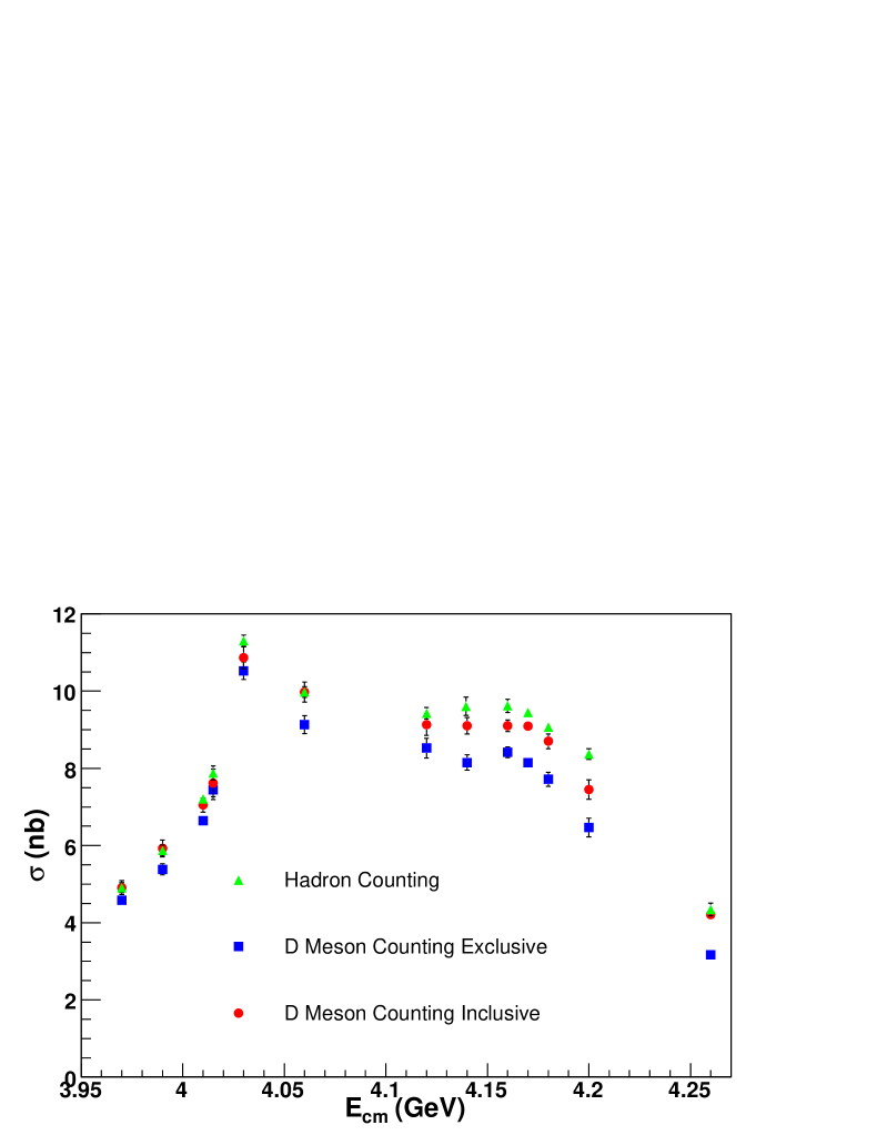
Figure 37: Plot of the total charm cross section as calculated in each of the three methods described in the text. The reason for the discrepancy between the inclusive and exclusive method is due to the presence of multi-body production, which is described in the text. Only statistical errors are shown.

Chapter Momentum Spectrum Analysis

10 Multi-Body, Initial-State Radiation, and
Momentum-Spectrum Fits

Throughout this analysis we have assumed that all charm production is through two-body events, that is $e^{+}e^{-}\rightarrow{D_{(s)}^{(*)}\bar{D}_{(s)}^{(*)}}$. With sufficient energy, however, there is no reason that final states like $e^{+}e^{-}\rightarrow{D\bar{D}^{(*)}\pi}$ or any other energetically allowed combination with extra pions should not be produced. From here on, these types of events are referred to as the multi-body production or just multi-body. For production of non-strange $D$ states, there is no a priori expectation for the amount of multi-body. For $D_{s}$ we expect it to be small, if not zero, since $D_{s}\bar{D}_{s}\pi$ violates isospin. In both cases it is appropriate to examine our data for evidence of such multi-body processes.

The first step is to determine whether multi-body exists. Assuming that it does, we then need to develop and apply procedures to determine its composition: $D\bar{D}\pi$, $D^{*}\bar{D}\pi$, or $D^{*}\bar{D}\pi\pi$.

To determine if multi-body exists we can apply tests of consistency between our measurements and the expectations for pure $D_{(s)}^{(*)}\bar{D}_{(s)}^{(*)}$ states. One observable is the ratio of $\frac{D^{0}}{D^{+}}$ as a function of energy, which is shown in Fig. 38. The bold horizontal lines are the predicted ratios as determined by the decays of the $D^{*}$ using the information in Table 11. It is evident that the observed ratio deviates from that expected for $D^{*}\bar{D}^{*}$ events. The only candidate explanation for this observation is multi-body production. The cut window in $M_{\rm{bc}}$ is different for neutral and charged $D^{*}$. The charged window is quite a bit smaller than the neutral, since the $\gamma$ decay is excluded when determining the cut window. Therefore, the cuts can select different amounts of the multi-body, which leads to a result which is not consistent with that expected based on known branching fractions. The fact that the $D^{*}\bar{D}$ events have the correct ratio will help in pin-pointing the make-up of the background.

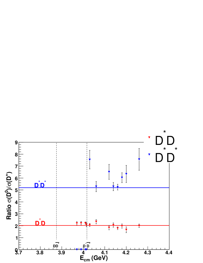
Figure 38: The measured ratio of $D^{0}$ to $D^{+}$ as a function of energy.

The ratio of $\frac{D^{0}}{D^{+}}$ gives a hint that there might be multi-body background present at the energies of interest, but it is far from conclusive. Another indication that points to a multi-body background is the noticeable difference in the total charm cross section between the exclusive and inclusive methods. The difference between these two methods as a function of energy can be seen in Fig. 37. The best way to prove the presence of multi-body is by looking for $D$ or $D^{*}$ mesons in a kinematically forbidden region. That is, we look for $D$ mesons in a momentum region where one would expect none under the assumption of pure two-body events. Fig. 39 shows a plot of the invariant mass of $D^{0}\rightarrow{K^{-}\pi^{+}}$ at the center-of-mass energy $4260$ MeV for $D^{0}$ candidates with momenta less than $300$ MeV/$c$. Under the assumption that only pure $D^{*}\bar{D}^{*}$, $D^{*}\bar{D}$, and $D\bar{D}$ are present, no $D^{0}$ are allowed below $\sim 500$ MeV/$c$. The figure shows a clearly defined peak at the $D^{0}$ mass, demonstrating the multi-body contribution.

Figure 39: The measured $D^{0}\rightarrow{K^{-}}\pi^{+}$ invariant mass distribution for $p_{D^{0}}<{300~{}{\rm{MeV/}}c}$. If the assumption of pure two-body events is made, then no $D^{0}$ decays are kinematically allowed below $\sim 500$ MeV/$c$ at $4260$ MeV.

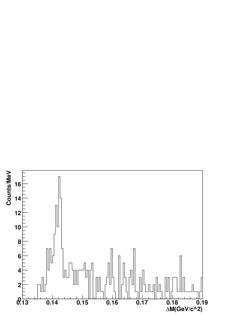
Figure 40: The measured $D^{*0}\rightarrow{D^{0}}\pi^{0}$ $\Delta$M distribution for $D^{0}\rightarrow{K^{-}}\pi^{+}$ satisfying $p_{D^{*0}}<{500~{}{\rm{MeV/}}c}$. If the assumption of pure two-body events is made, then no $D^{*0}$ decays are kinematically allowed below $\sim 700$ MeV/$c$ at $4260$ MeV.

This demonstrates that charm is produced through more than the two-body event categories, but it sheds no light on the composition. Are the multi-body events $D\bar{D}\pi$, $D\bar{D}\pi\pi$, $D^{*}\bar{D}\pi$, etc., or a combination of all possible types? To help answer this question a similar study to the one above, was performed for $D^{*0}$. Fig. 40 shows a plot of the $\Delta$M spectrum for $p_{D^{*0}}<{500~{}{\rm{MeV/}}c}$. If the assumption of only pure two-body events is made, then no $D^{*0}$ decays are kinematically allowed below $\sim 700$ MeV/$c$. The figure clearly shows that there exist multi-body events of the type $D^{*}\bar{D}\pi$ in the data, evident in the well-defined peak located at $\Delta{M}=M_{D^{*0}}-M_{D^{0}}=0.142~{}{\rm{MeV/}}c^{2}$.

Looking in the kinematically forbidden region has given clues to the possible composition of the multi-body events, but still does not provide a definitive and quantitative breakdown. One reason is that initial-state radiation (ISR), can lead to $D$ mesons smeared outside of the two-body kinematic regions. A more definitive test is to reconstruct a $D^{*}$, add a charged or neutral $\pi$, and look at the missing mass (recoil mass) of the event. A peak in the missing mass at the $D$ would clearly demonstrate the presence of $D^{*}\bar{D}\pi$ in the data. We concentrate on multi-body events of the type $D^{(*)0}D^{\pm}\pi^{\mp}$, which by isospin are twice as likely to occur as $D^{(*)0}\bar{D^{0}}\pi^{0}$ and $D^{(*)+}\bar{D^{-}}\pi^{0}$. In addition to the factor of two from isospin, the multi-body events with a charged pion should be cleaner than those with a neutral pion, since the additional pion will be soft, $P_{\pi}<{150}$ MeV/$c$. With this method the observation of multi-body cannot be obscured by ISR, because the presence of the radiative photon will prohibit peaks in the missing-mass spectrum.

For this study we use the high-statistics data sample collected at 4170 MeV, consisting of 179 pb^-1. Using $D^{*+}\rightarrow{D^{+}}\pi^{0}$ with $D^{+}\rightarrow{K^{-}}\pi^{+}\pi^{+}$, and $D^{*0}\rightarrow{D^{0}}\pi^{0}$ with $D^{0}\rightarrow{K^{-}}\pi^{+}$, $D^{0}\rightarrow{K^{-}}\pi^{+}\pi^{0}$, or $D^{0}\rightarrow{K^{-}}\pi^{+}\pi^{+}\pi^{-}$, in addition to DTAG-like cuts for the charged pion, we obtain the missing-mass spectra shown in Figs. 41 and 42.

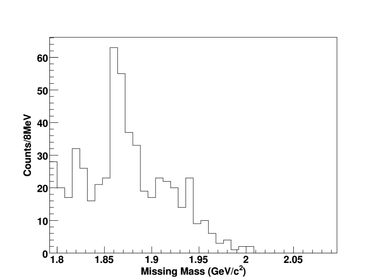
Figure 41: The mass spectrum of $X$, in $e^{+}e^{-}\rightarrow{D^{*\pm}\pi^{\mp}X}$, using the $179~{}{\rm{pb}}^{-1}$ collected at $4170$ MeV. The peak at the $D$ mass shows conclusive evidence that events of the form $D^{*}\bar{D}\pi$ are present in the data. A cut on the reconstructed $D^{*}$ momentum of 400 ${\rm{MeV}/}c$ was used to exclude two-body events.

Fig. 41 is the invariant mass spectrum of $X$ in $e^{+}e^{-}\rightarrow{D^{*\pm}\pi^{\mp}X}$, while Fig. 42 is for $X$ in $e^{+}e^{-}\rightarrow{D^{*0}\pi^{\pm}X}$, where for the latter decay the charge of the $D$-daughter kaon is used to obtain the correct combination of the neutral $D^{*}$ and the charged pion. For both cases we define the signal region as a 6 MeV window centered on the previously measured (PDG) mass difference. A cut on the reconstructed $D^{*}$ momentum of 400 ${\rm{MeV}/}c$ was used to exclude two-body events. These figures provide conclusive evidence that multi-body events of the form $D^{*}\bar{D}\pi$ exist in the data. We must now determine the amount of multi-body present to assess the effect on the two-body cross sections that were determined earlier.

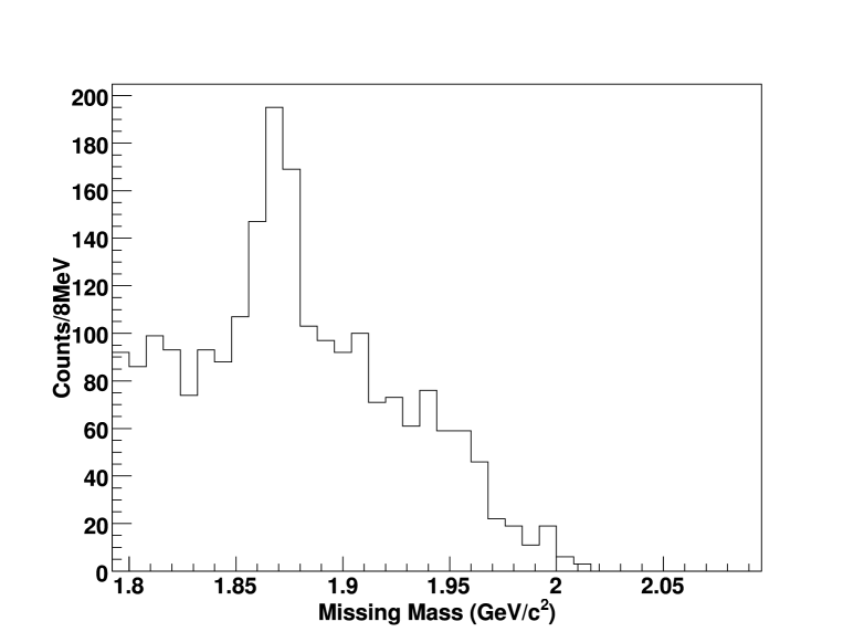
Figure 42: The mass spectrum of $X$, in $e^{+}e^{-}\rightarrow{D^{*0}\pi^{\pm}X}$, using the $179~{}{\rm{pb}}^{-1}$ collected at $4170$ MeV. The peak at the $D$ mass shows conclusive evidence for production of $D^{*}\bar{D}\pi$ events. A cut on the reconstructed $D^{*}$ momentum of 400 ${\rm{MeV}/}c$ was used to exclude two-body events. In addition, the charge of the $D$-daughter kaon is used to obtain the correct combination of the neutral $D^{*}$ and the charged pion.

We performed a similar study with the data collected at 4260 MeV. The corresponding missing-mass spectrum, only for $D^{*0}\rightarrow{D^{0}\pi^{0}}$ with $D^{0}\rightarrow{K^{-}}\pi^{+}$, $D^{0}\rightarrow{K^{-}}\pi^{+}\pi^{0}$, or $D^{0}\rightarrow{K^{-}}\pi^{+}\pi^{+}\pi^{-}$, is shown in Fig. 43 for the $13.11~{}{\rm{pb}}^{-1}$ collected at $4260$ MeV. A cut of 500 ${\rm{MeV}/}c$ was made on the reconstructed $D^{*}$ momentum to select entries from the multi-body region. In addition, the charge of the $D$-daughter kaon is used to obtain the correct combination of the neutral $D^{*}$ and the charged pion. It is clear from the plot that $D^{*}\bar{D}^{*}\pi$ multi-body events exist, in addition to $D^{*}\bar{D}\pi$, at 4260 MeV. This is shown by the clear peaks at both the $D$ and the $D^{*}$ masses in Fig. 43.

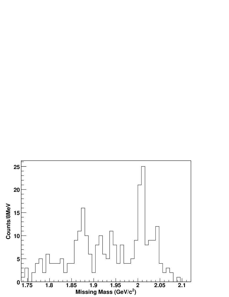
Figure 43: Mass spectrum for $X$, in $e^{+}e^{-}\rightarrow{D^{*0}\pi^{\mp}X}$, at 4260 MeV. The charge of the daughter kaon is used to obtain the correct combination of the neutral $D$ and the charged pion. The peak at the $D$ mass is additional evidence of the existence of $D^{*}D\pi$, whereas the peak at the $D^{*}$ mass is evidence of the production of $D^{*}D^{*}\pi$. A cut of 500 ${\rm{MeV}/}c$ was made on the reconstructed $D^{*}$ momentum to select entries from the multi-body region.

Having demonstrated unambiguously that events of the form $D^{*}\bar{D}\pi$ are present in our energy region, it remains to be determined if other types of events, like $D\bar{D}\pi$, also contribute. We performed a similar study to the one above using a $D$ rather than a $D^{*}$ to investigate this possibility in the 4170 MeV data sample. Using only $D^{0}\rightarrow{K^{-}}\pi^{+}$ and $D^{+}\rightarrow{K^{-}}\pi^{+}\pi^{+}$, in addition to another charged pion, we obtained the missing-mass spectra in Figs. 44 and 45. Fig. 44 shows the mass of $X$ in $e^{+}e^{-}\rightarrow{D^{\pm}\pi^{\mp}X}$, while Fig. 45 gives the mass of $X$ in $e^{+}e^{-}\rightarrow{D^{0}\pi^{\mp}X}$.

Figure 44: The mass spectrum of $X$, in $e^{+}e^{-}\rightarrow{D^{\pm}\pi^{\mp}X}$, using the $179~{}{\rm{pb}}^{-1}$ collected at $4170$ MeV. A cut on the reconstructed $D$ momentum of 250 ${\rm{MeV}/}c$ was made to exclude two-body events. The peak at the $D^{*}$ mass shows, again, conclusive evidence for events of the form $D^{*}\bar{D}\pi$ being present in the data. The lack of a peak at the $D$ mass shows the lack of $D\bar{D}\pi$ type events in the data.

For the latter decay we use the charge of the $D$-daughter kaon to obtain the correct combination of the neutral $D$ and the charged pion. In both plots, the signal region is defined to be a 30-MeV window centered on the known $D$ mass. A cut on the reconstructed $D$ momentum of 250 ${\rm{MeV}/}c$ was made to exclude two-body events. In both Figs. 44 and 45, clear peaks at the $D^{*}$ mass give further evidence for $D^{*}\bar{D}\pi$ multi-body events. The absence of a peak at the $D$ mass indicates that there is no evidence for $D\bar{D}\pi$ production, although such a contribution may still be present in the data and suppressed by the $D$-momentum cut.

Figure 45: The mass spectrum of $X$, in $e^{+}e^{-}\rightarrow{D^{0}\pi^{\pm}X}$, using the $179~{}{\rm{pb}}^{-1}$ collected at $4170$ MeV. A cut on the reconstructed $D$ momentum of 250 ${\rm{MeV}/}c$ was made to exclude two-body events. In addition, the charge of the $D$-daughter kaon is used to obtain the correct combination of the neutral $D^{*}$ and the charged pion. The peak at the $D^{*}$ mass shows further evidence for events of the form $D^{*}\bar{D}\pi$. The absence of a peak at the $D$ mass indicates the lack of $D\bar{D}\pi$ events in the data.

Now that the components of the multi-body have been identified, a method to measure its yield is needed so that we can correct the exclusive $D^{*}\bar{D}^{*}$ and total exclusive charm cross sections for the portion of the multi-body that was excluded. To accomplish this, we use a two-body MC representation of the various exclusive channels and a spin-averaged phase-space model MC representation of $D^{*}\bar{D}\pi$, and $D^{*}\bar{D}^{*}\pi$, and fit the sideband-subtracted momentum spectrum for $D^{0}\rightarrow{K^{-}}\pi^{+}$.

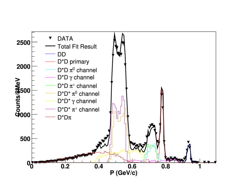
Figure 46: Sideband-subtracted momentum spectrum for $D^{0}\rightarrow{K^{-}}\pi^{+}$ at 4170 MeV. Data are shown as the points with error bars which are fit to the MC (histograms). The fit uses a spin-averaged phase-space model MC representation of $D^{*}\bar{D}\pi$, shown in dark red. The fit seems to replicate the overall structure reasonable well, but is clearly deficient in some regions.

In the sideband-subtraction method the signal region, in invariant mass, is defined to be $\pm 3\sigma$, where $\sigma$ is 5 MeV, about the PDG mass. The low-side and high-side sidebands start at 7.5 $\sigma$ away from the peak and extend outward by 3 $\sigma$. The reconstructed $D$ momentum for each region is plotted and the resulting histograms are subtracted. The fit made at 4170 MeV is shown in Fig. 46. The fit seems to replicate the overall structure reasonably well, but is clearly lacking in some regions.

Besides fitting the $D^{0}\rightarrow{K^{-}}\pi^{+}$ momentum spectrum, a fit to the $D^{+}\rightarrow{K^{-}}\pi^{+}\pi^{+}$ can be a good cross-check and test of the method. Fig. 47 shows this test using all the assumptions made up to this point. The fit is not as good as the $D^{0}$, and it is clear that that something is missing. The disagreement between the fit and the data is dramatic between 600 and 750 ${\rm{MeV}}/c$.

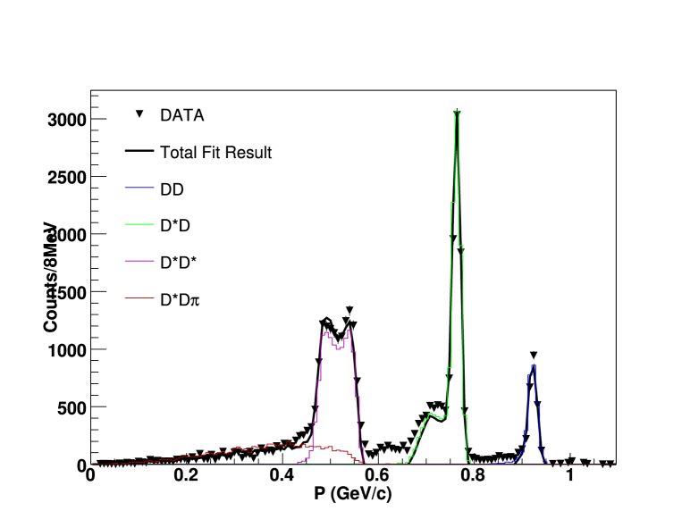
Figure 47: Sideband-subtracted momentum spectrum for $D^{+}\rightarrow{K^{-}}\pi^{+}\pi^{+}$ at 4170 MeV. Data are shown as points with error bars which are fit to the MC (histograms). The fit uses a spin-averaged phase-space model MC representation of $D^{*}\bar{D}\pi$, shown in dark red. There is a large discrepancy between what is expected and what is seen around 600-750 ${\rm{MeV}}/c$. This discrepancy suggests that $D\bar{D}\pi$ may be present at this energy.

We considered three possible explanations for this discrepancy: (1) the branching fraction for the gamma decay channel is wrong, (2) $D\bar{D}\pi$ is present in the data; and (3) something more fundamental is missing. The first possibility seems unlikely, because enhancements are not seen in the region around $D^{*+}D^{*-}$ outside that of the $\pi^{0}$ enhancement, like those seen in the $D^{0}\rightarrow{K^{-}}\pi^{+}$ spectrum. The second possibility seems more likely since all the searches for multi-body thus far only looked in momentum regions that limited the allowable amount of $D\bar{D}\pi$. If we take Fig. 47 as evidence for the presence of $D\bar{D}\pi$, we can modify our fit procedure to allow a $D\bar{D}\pi$ contribution. This greatly improves the fit quality, which can be seen in Fig. 48 for $D^{0}\rightarrow{K^{-}}\pi^{+}$ and Fig. 49 for $D^{+}\rightarrow{K^{-}}\pi^{+}\pi^{+}$.

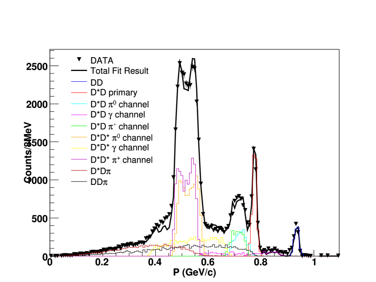
Figure 48: Sideband-subtracted momentum spectrum for $D^{0}\rightarrow{K^{-}}\pi^{+}$ at 4170 MeV. Data are shown as points with error bars which are fit to the MC (histograms). The fit uses a spin-averaged phase-space model MC representation for $D^{*}\bar{D}\pi$, shown in dark red, and $D\bar{D}\pi$ is shown in black.

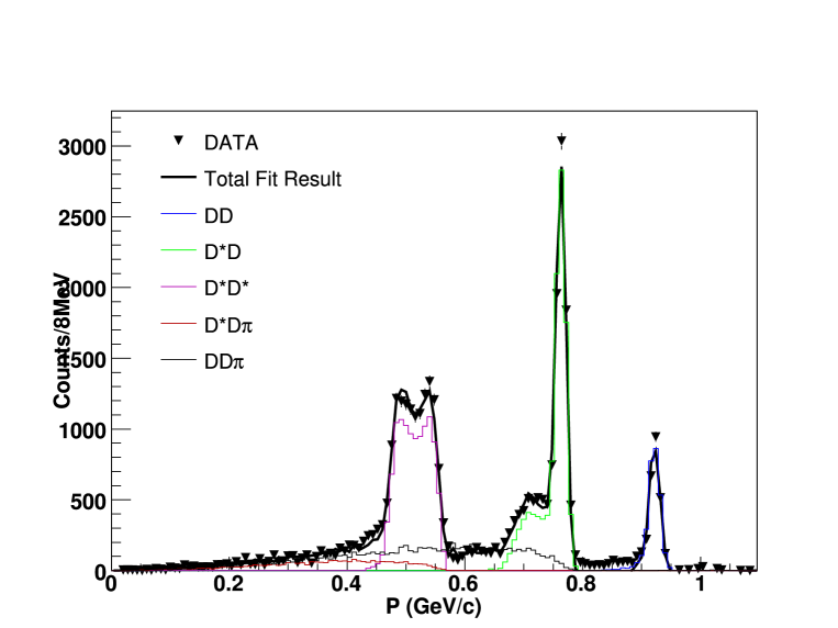
Figure 49: Sideband-subtracted momentum spectrum for $D^{+}\rightarrow{K^{-}}\pi^{+}\pi^{+}$ at 4170 MeV. Data are shown as points with error bars which are fit to the MC (histograms). The fit uses a spin-averaged phase-space model MC representation for $D^{*}\bar{D}\pi$, shown in dark red, and $D\bar{D}\pi$ is shown in black.

While the fits are improved, we find large discrepancies in the $D^{0}/D^{+}$ ratio for $D^{*}\bar{D}\pi$ using the composition obtained from the fits. The ratio of $\sigma(D^{0})_{D^{*}\bar{D}\pi}$ to $\sigma(D^{+})_{D^{*}\bar{D}\pi}$ should be 2, while the result from the fit is about 5. Also, the ratio of $\sigma(D^{0})_{D\bar{D}\pi}$ to $\sigma(D^{+})_{D\bar{D}\pi}$ should be 1, but the result from the fit is about 2. So even though the fits look good, the corresponding results are not consistent and further investigation is warranted.

Using all the data collected at 4170 MeV, it is possible to break down the ratio of $D^{0}$ to $D^{+}$ as a function of energy. The ratio can be seen in Fig. 50.

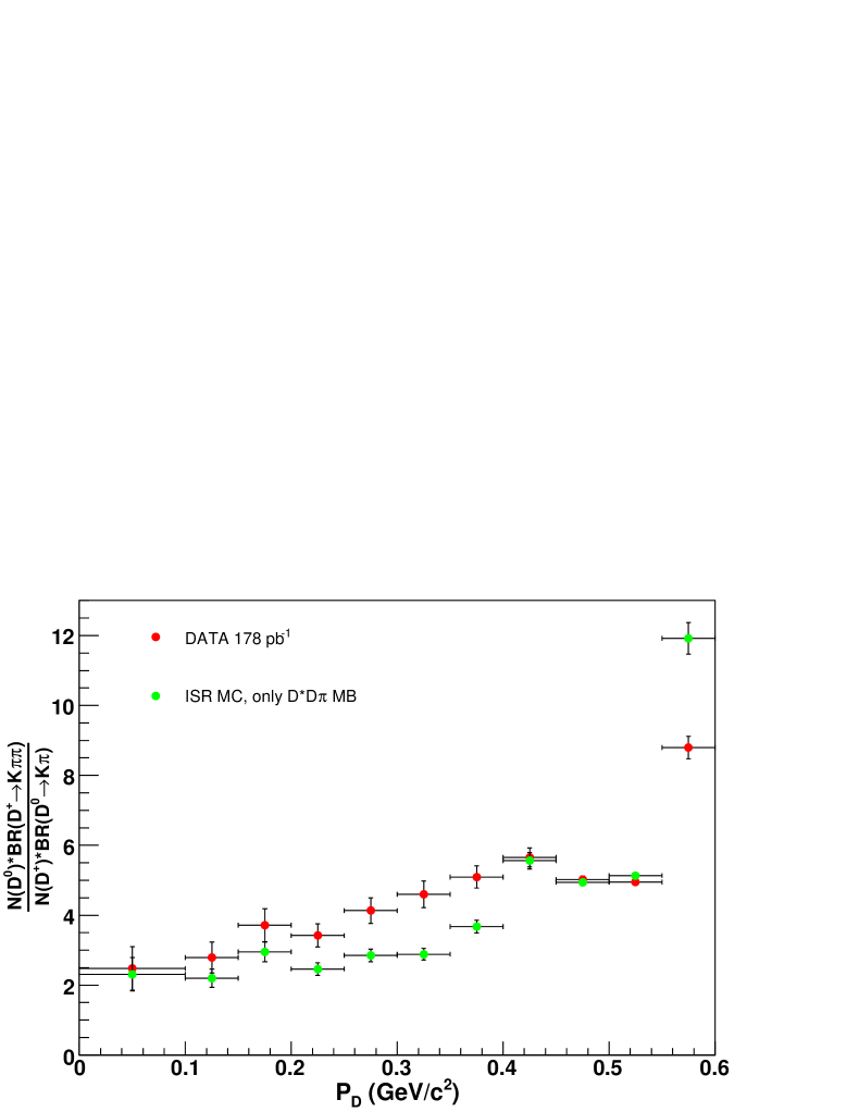
Figure 50: Ratio of the number of $D^{0}$ to $D^{+}$ as a function of reconstructed $D$ momentum at $E_{{\rm{cm}}}=4170$ MeV. The differences in the branching fractions were included in the ratio, while the efficiencies were take to be constant over the momentum range. The MC includes only $D^{*}\bar{D}\pi$ multi-body production and uses a simple ISR model that assumes all events are produced from the $\psi(4160)$ resonance, with a width of 78 MeV. The large discrepancy between the data and the MC between 200 and 400 MeV/$c$ clearly indicates that something is incorrect in our assumptions used to generate the MC sample.

Notice that the ratio is not corrected for efficiency, which is found with MC to be constant across the momentum range. Fig. 50 shows the ratio both for the 4170 MeV data set and for a MC sample that only assumes $D^{*}\bar{D}\pi$ multi-body and implements a simple model for the effects of ISR. The ISR model treats all charm production as coming from the $\psi(4160)$ resonance, which has a width of 78 MeV [2]. There is a large discrepancy between the MC and data in the momentum range 200-400 MeV/$c$. This discrepancy would be even worse if $D\bar{D}\pi$ were added to the MC. While this particular model does solve the problem of the discrepancies seen in the momentum fits, it does suggest the need for improvements in our MC.

To investigate further, we similarly computed the ratio of $D^{*0}$ to $D^{*+}$, again not correcting for efficiency, which is found to be constant across the momentum range. The result is shown in Fig. 51.

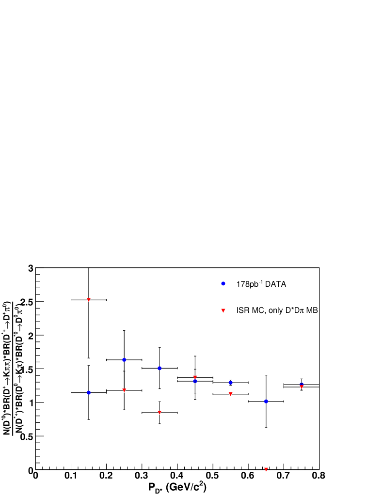
Figure 51: Ratio of $D^{*0}$ to $D^{*+}$, both using the $\pi^{0}$ channel, with the subsequent $D$-meson decays $D^{0}\rightarrow{K^{-}}\pi^{+}$ and $D^{+}\rightarrow{K^{-}}\pi^{+}\pi^{+}$, respectively. The ratio includes the branching fractions but excludes the efficiencies, which are constant over the momentum range. The MC includes only $D^{*}\bar{D}\pi$ multi-body production and uses a simple ISR model that assumes all events are produced from the $\psi(4160)$ resonance, with a width of 78 MeV. The discrepancy at 650 MeV/$c$ indicates that ISR is important and that it is incorrectly handled in our MC sample.

The same MC sample with a simple resonance model is used. The most surprising result can be seen at 650 MeV/$c$ in the region between the peaks for the two-body events $D^{*}\bar{D}^{*}$ and $D\bar{D}^{*}$. In the limit of perfect resolution, there should be two delta functions, one for $D^{*}$ in $D^{*}\bar{D}$ events and one $D^{*}$ in $D^{*}\bar{D}^{*}$ events, where the 650 MeV/$c$ bin falls right in the middle. This is true even accounting for resolution, and therefore, the ratio should be zero. That this ratio is zero for MC but not data demonstrates that our simple ISR MC is incorrect and a better model is needed.

Our improved approach is to use EVTGEN’s model of EvtVPHOtoVISR [57], representing the cross sections for each event type of two-body events (Figs. 32 and 33) with simple linear interpolations between our measured data points, as is shown in Figs. 52 and 53. For multi-body constant cross sections are assumed. Momentum fits to these models give the results for $D^{0}\rightarrow{K^{-}}\pi^{+}$ and $D^{+}\rightarrow{K^{-}}\pi^{+}\pi^{+}$ shown in Fig. 54 and Fig. 55, respectively. In addition to fitting $D^{0}$ and $D^{+}$, one can fit the $D_{s}$ momentum distribution using the same procedure. This result, only for $D_{s}^{+}\rightarrow\phi\pi^{+}$, is given in Fig. 56.

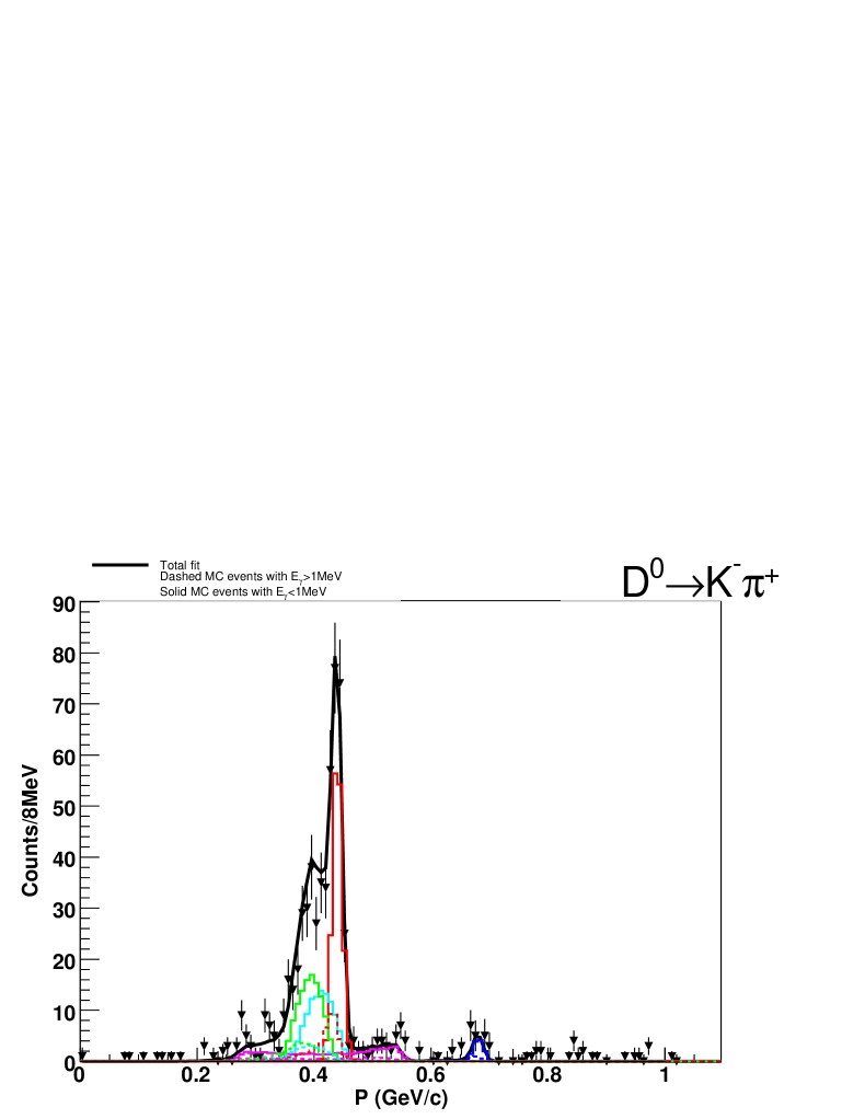
Figure 87: Sideband-subtracted momentum spectrum for $D^{0}\rightarrow{K^{-}}\pi^{+}$ at 3970 MeV. The data is the points with error bars and the histograms are MC.

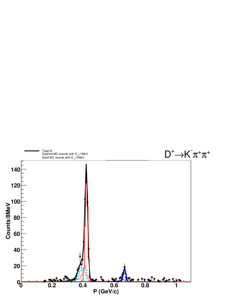
Figure 88: Sideband-subtracted momentum spectrum for $D^{+}\rightarrow{K^{-}}\pi^{+}\pi^{+}$ at 3970 MeV. The data is the points with error bars and the histograms are MC.

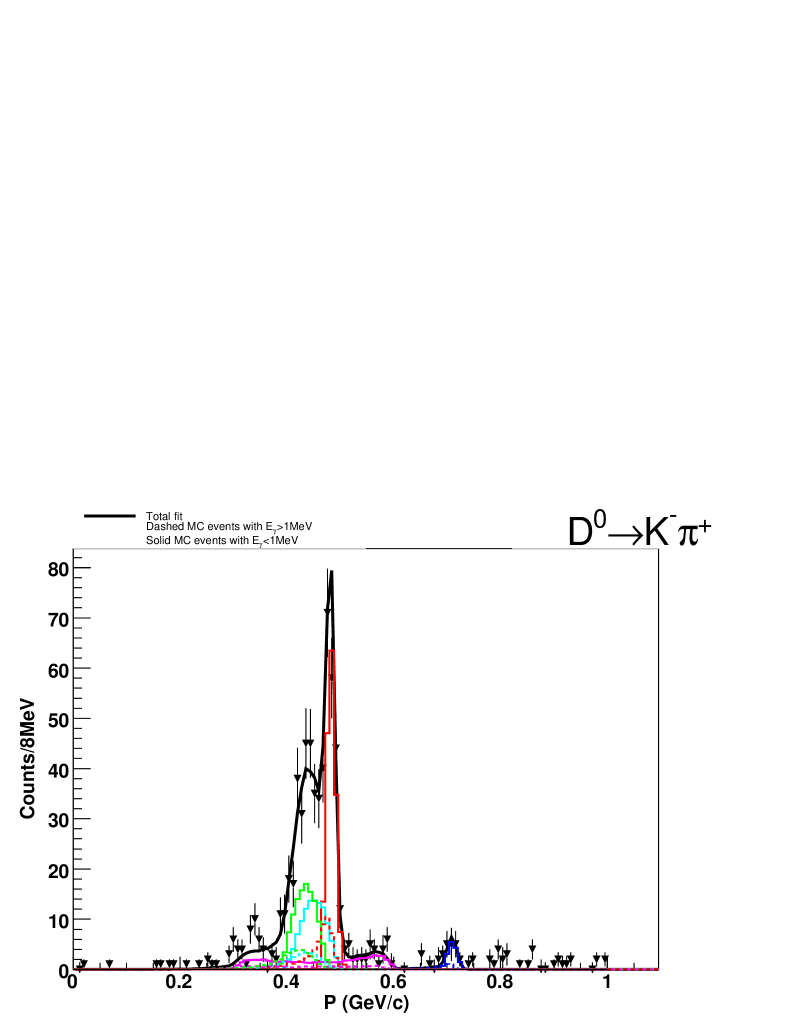
Figure 89: Sideband-subtracted momentum spectrum for $D^{0}\rightarrow{K^{-}}\pi^{+}$ at 3990 MeV. The data is the points with error bars and the histograms are MC.

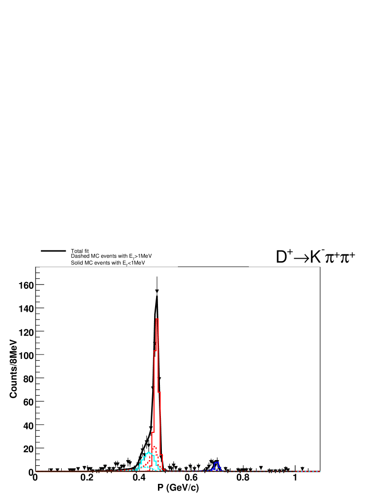
Figure 90: Sideband-subtracted momentum spectrum for $D^{+}\rightarrow{K^{-}}\pi^{+}\pi^{+}$ at 3990 MeV. The data is the points with error bars and the histograms are MC.

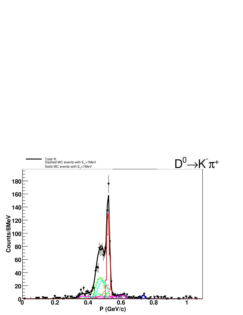
Figure 91: Sideband-subtracted momentum spectrum for $D^{0}\rightarrow{K^{-}}\pi^{+}$ at 4010 MeV. The data is the points with error bars and the histograms are MC.

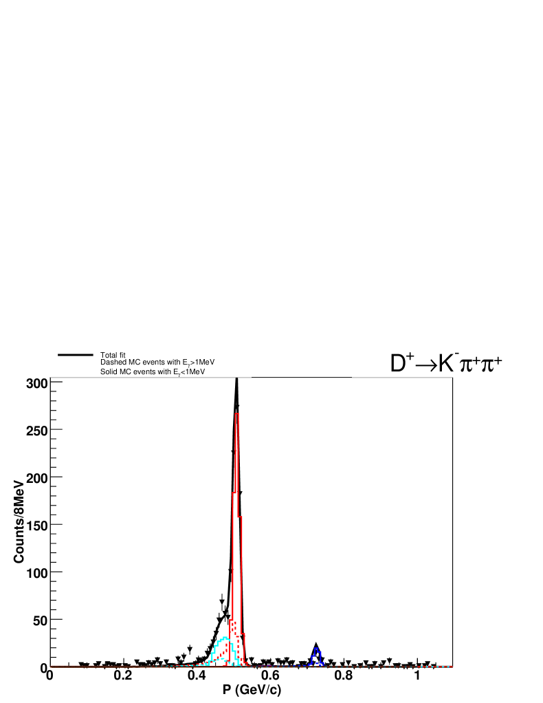
Figure 92: Sideband-subtracted momentum spectrum for $D^{+}\rightarrow{K^{-}}\pi^{+}\pi^{+}$ at 4010 MeV. The data is the points with error bars and the histograms are MC.

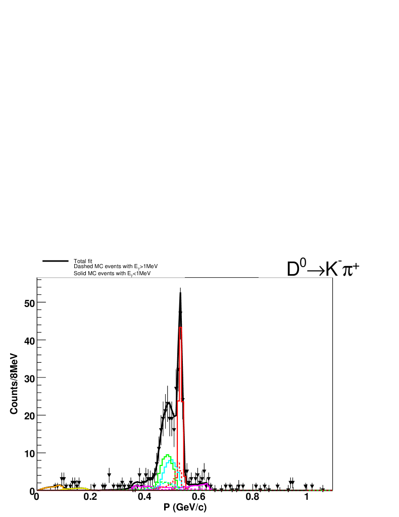
Figure 93: Sideband-subtracted momentum spectrum for $D^{0}\rightarrow{K^{-}}\pi^{+}$ at 4015 MeV. The data is the points with error bars and the histograms are MC.

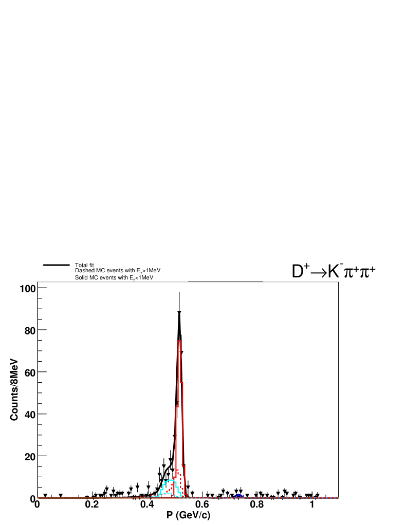
Figure 94: Sideband-subtracted momentum spectrum for $D^{+}\rightarrow{K^{-}}\pi^{+}\pi^{+}$ at 4015 MeV. The data is the points with error bars and the histograms are MC.

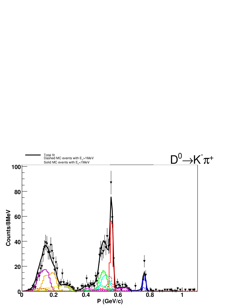
Figure 95: Sideband-subtracted momentum spectrum for $D^{0}\rightarrow{K^{-}}\pi^{+}$ at 4030 MeV. The data is the points with error bars and the histograms are MC.

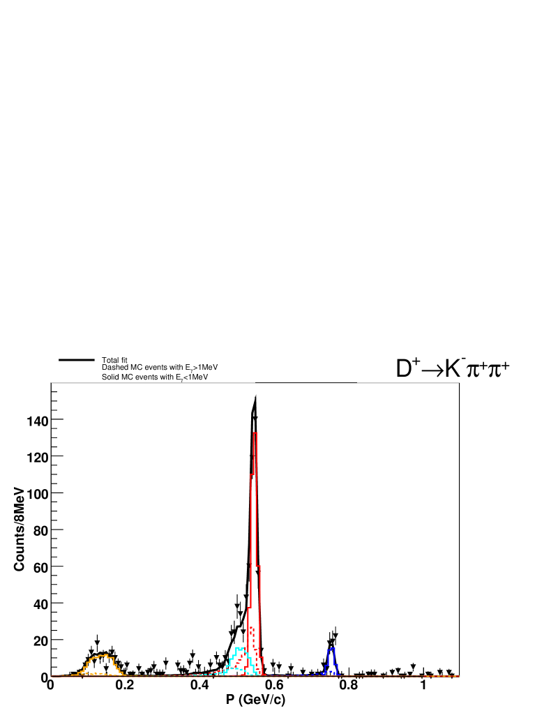
Figure 96: Sideband-subtracted momentum spectrum for $D^{+}\rightarrow{K^{-}}\pi^{+}\pi^{+}$ at 4030 MeV. The data is the points with error bars and the histograms are MC.

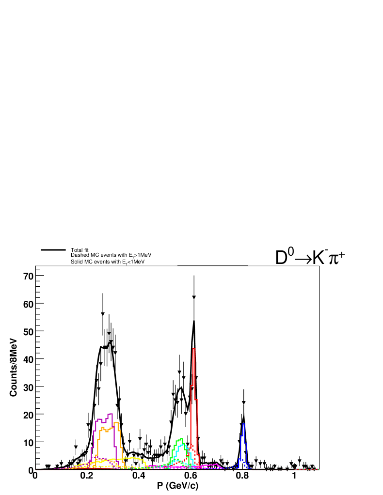
Figure 97: Sideband-subtracted momentum spectrum for $D^{0}\rightarrow{K^{-}}\pi^{+}$ at 4060 MeV. The data is the points with error bars and the histograms are MC.

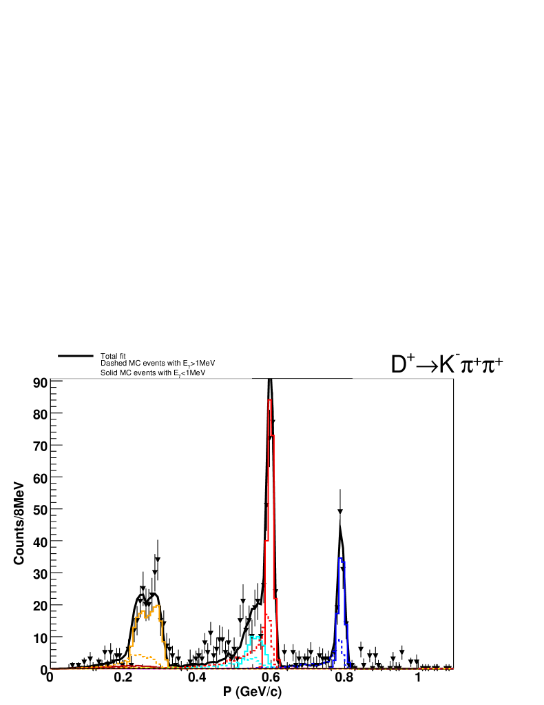
Figure 98: Sideband-subtracted momentum spectrum for $D^{+}\rightarrow{K^{-}}\pi^{+}\pi^{+}$ at 4060 MeV. The data is the points with error bars and the histograms are MC.

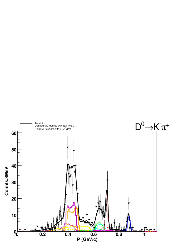
Figure 99: Sideband-subtracted momentum spectrum for $D^{0}\rightarrow{K^{-}}\pi^{+}$ at 4120 MeV. The data is the points with error bars and the histograms are MC.

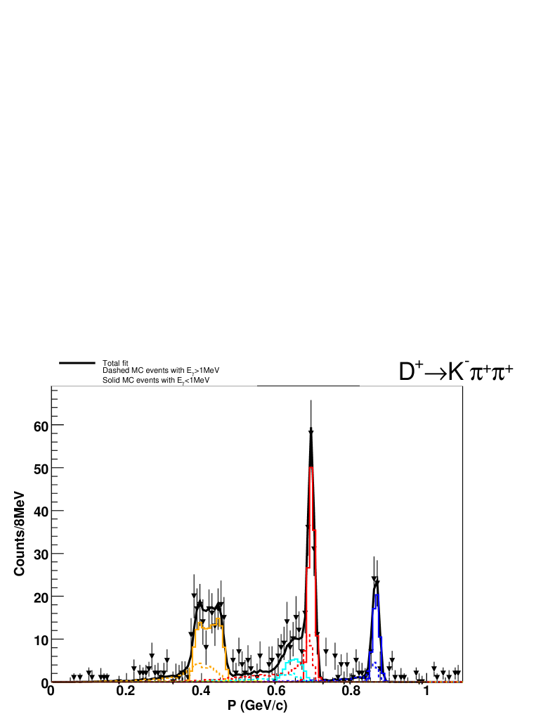
Figure 100: Sideband-subtracted momentum spectrum for $D^{+}\rightarrow{K^{-}}\pi^{+}\pi^{+}$ at 4120 MeV. The data is the points with error bars and the histograms are MC.

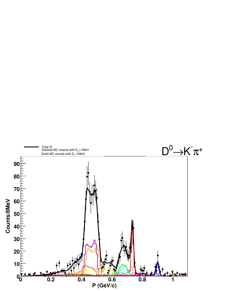
Figure 101: Sideband-subtracted momentum spectrum for $D^{0}\rightarrow{K^{-}}\pi^{+}$ at 4140 MeV. The data is the points with error bars and the histograms are MC.

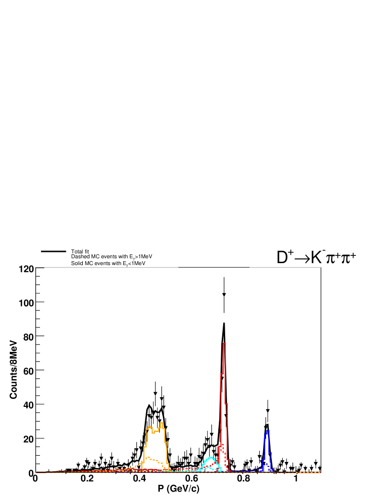
Figure 102: Sideband-subtracted momentum spectrum for $D^{+}\rightarrow{K^{-}}\pi^{+}\pi^{+}$ at 4140 MeV. The data is the points with error bars and the histograms are MC.

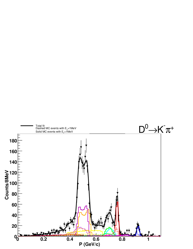
Figure 103: Sideband-subtracted momentum spectrum for $D^{0}\rightarrow{K^{-}}\pi^{+}$ at 4160 MeV. The data is the points with error bars and the histograms are MC.

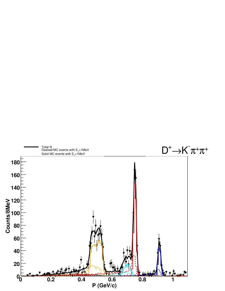
Figure 104: Sideband-subtracted momentum spectrum for $D^{+}\rightarrow{K^{-}}\pi^{+}\pi^{+}$ at 4160 MeV. The data is the points with error bars and the histograms are MC.

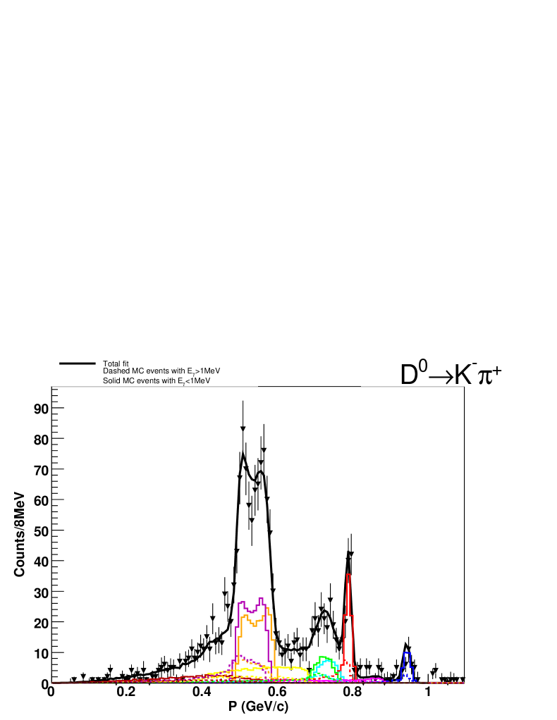
Figure 105: Sideband-subtracted momentum spectrum for $D^{0}\rightarrow{K^{-}}\pi^{+}$ at 4180 MeV. The data is the points with error bars and the histograms are MC.

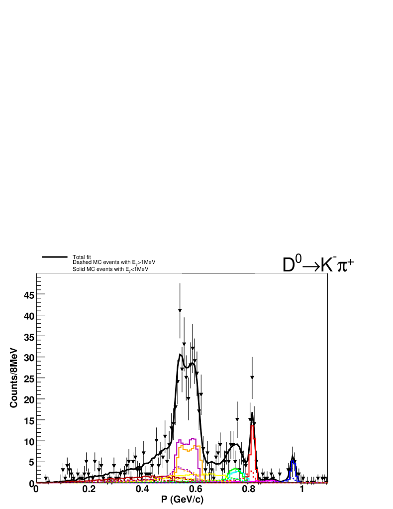
Figure 107: Sideband-subtracted momentum spectrum for $D^{0}\rightarrow{K^{-}}\pi^{+}$ at 4200 MeV. The data is the points with error bars and the histograms are MC.

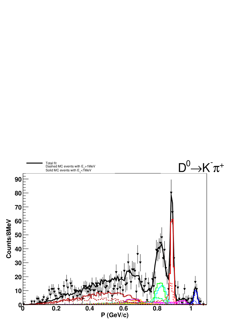
Figure 109: Sideband-subtracted momentum spectrum for $D^{0}\rightarrow{K^{-}}\pi^{+}$ at 4260 MeV. The data is the points with error bars and the histograms are MC.

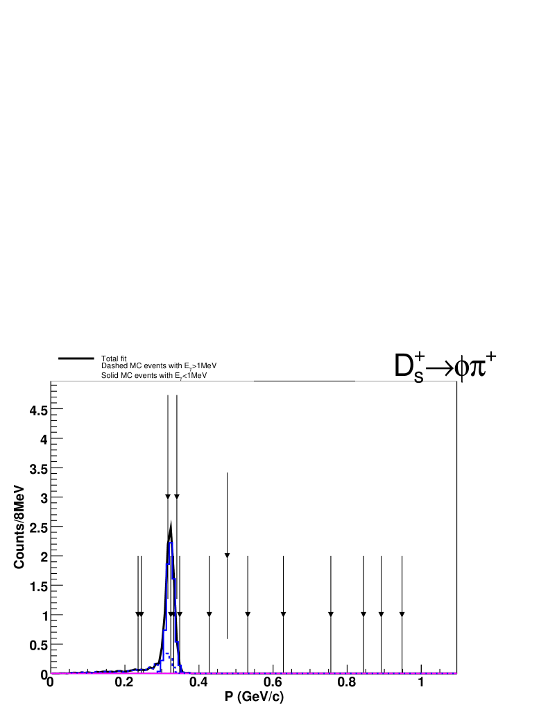
Figure 112: Sideband-subtracted momentum spectrum for $D_{s}^{+}\rightarrow\phi\pi^{+}$ at 3990 MeV. The data is the points with error bars and the histograms are MC.

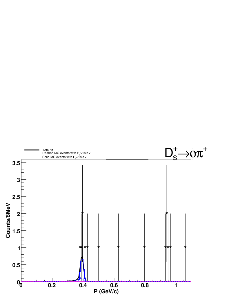
Figure 114: Sideband-subtracted momentum spectrum for $D_{s}^{+}\rightarrow\phi\pi^{+}$ at 4015 MeV. The data is the points with error bars and the histograms are MC.

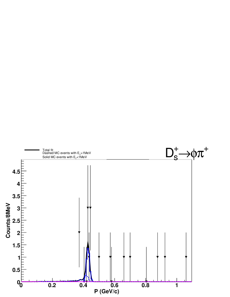
Figure 115: Sideband-subtracted momentum spectrum for $D_{s}^{+}\rightarrow\phi\pi^{+}$ at 4030 MeV. The data is the points with error bars and the histograms are MC.

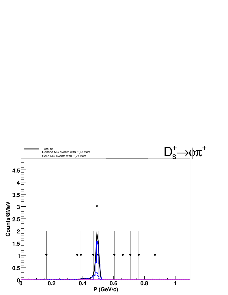
Figure 116: Sideband-subtracted momentum spectrum for $D_{s}^{+}\rightarrow\phi\pi^{+}$ at 4060 MeV. The data is the points with error bars and the histograms are MC.

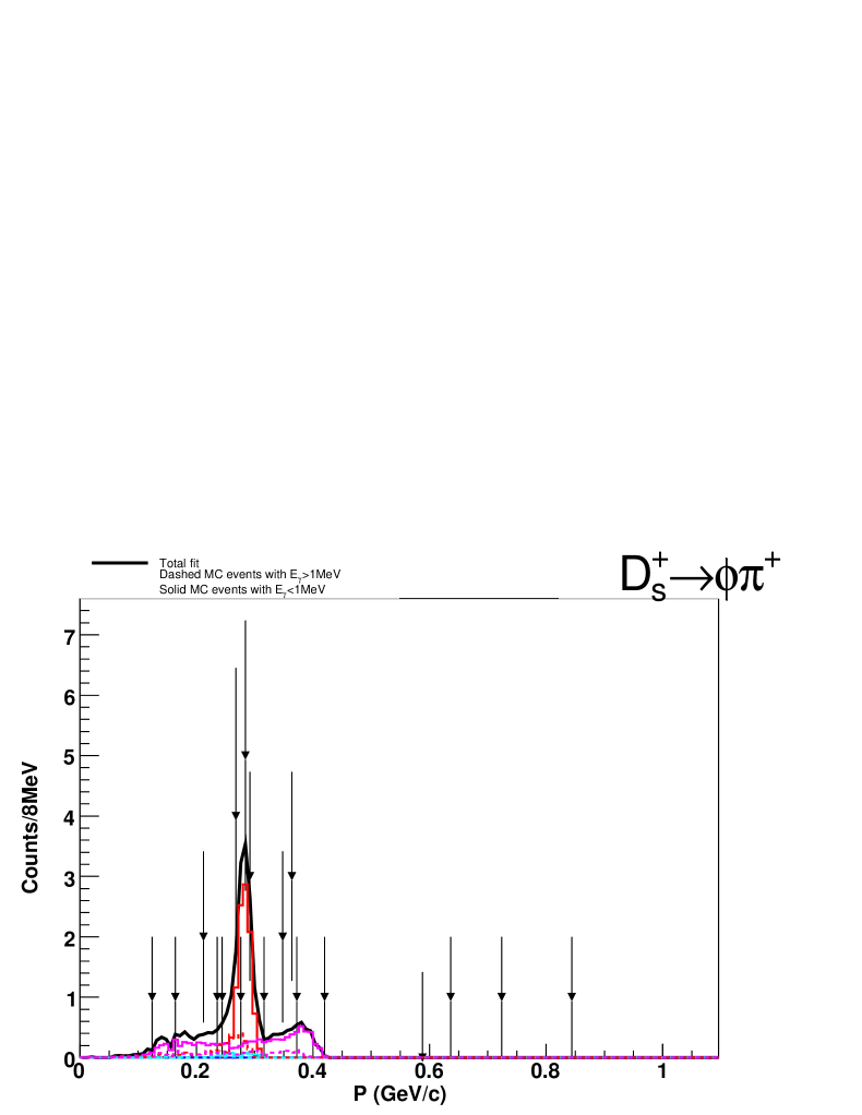
Figure 117: Sideband-subtracted momentum spectrum for $D_{s}^{+}\rightarrow\phi\pi^{+}$ at 4120 MeV. The data is the points with error bars and the histograms are MC.

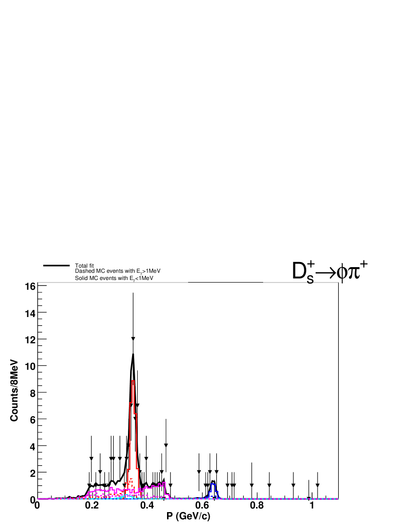
Figure 118: Sideband-subtracted momentum spectrum for $D_{s}^{+}\rightarrow\phi\pi^{+}$ at 4140 MeV. The data is the points with error bars and the histograms are MC.

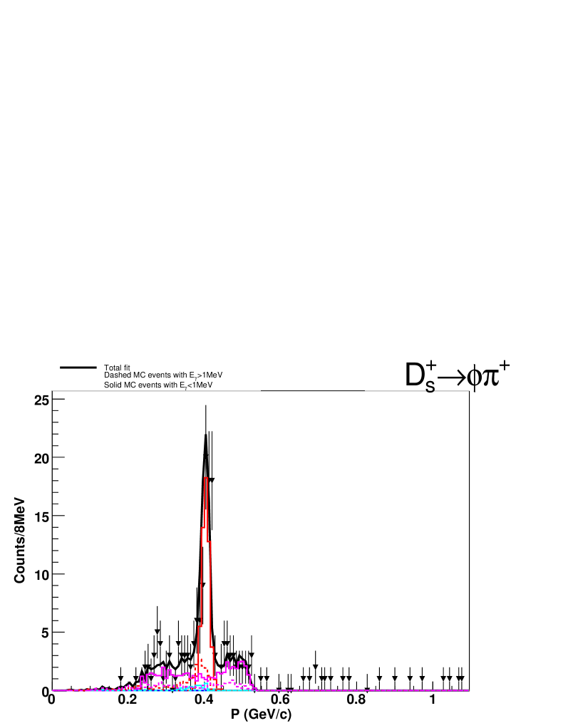
Figure 119: Sideband-subtracted momentum spectrum for $D_{s}^{+}\rightarrow\phi\pi^{+}$ at 4160 MeV. The data is the points with error bars and the histograms are MC.

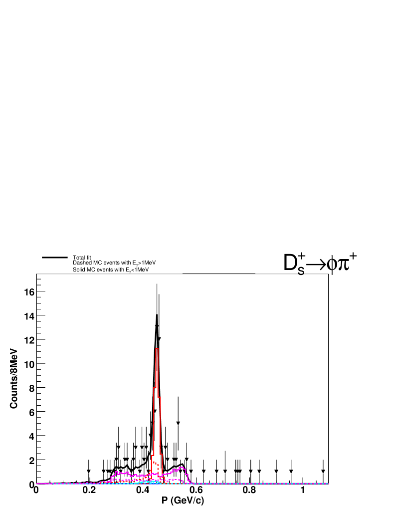
Figure 120: Sideband-subtracted momentum spectrum for $D_{s}^{+}\rightarrow\phi\pi^{+}$ at 4180 MeV. The data is the points with error bars and the histograms are MC.

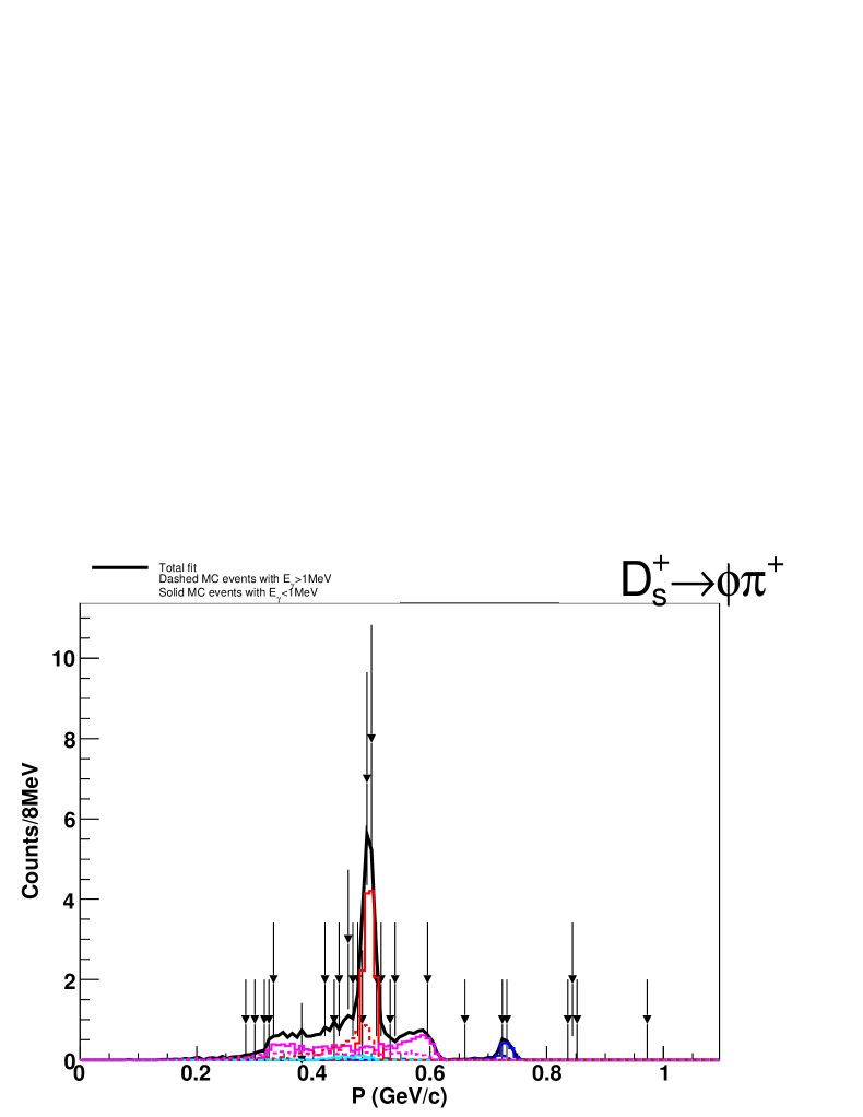
Figure 121: Sideband-subtracted momentum spectrum for $D_{s}^{+}\rightarrow\phi\pi^{+}$ at 4200 MeV. The data is the points with error bars and the histograms are MC.

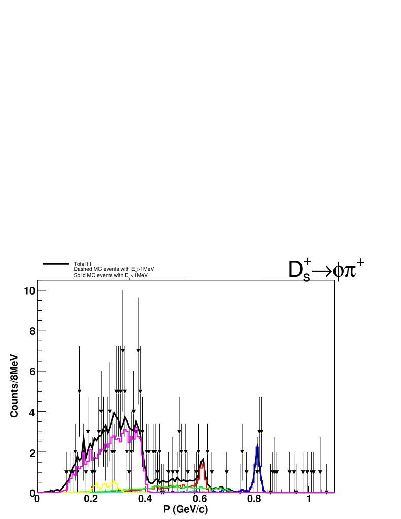
Figure 122: Sideband-subtracted momentum spectrum for $D_{s}^{+}\rightarrow\phi\pi^{+}$ at 4260 MeV. The data is the points with error bars and the histograms are MC.

Momentum-spectrum fits for data collected at other energy points are shown in Figs. 87-109 for $D^{0}$ and $D^{+}$ and Figs. 111-122 for $D_{s}$. It is interesting to see the emergence of the various final states as the center-of-mass energy is increased.

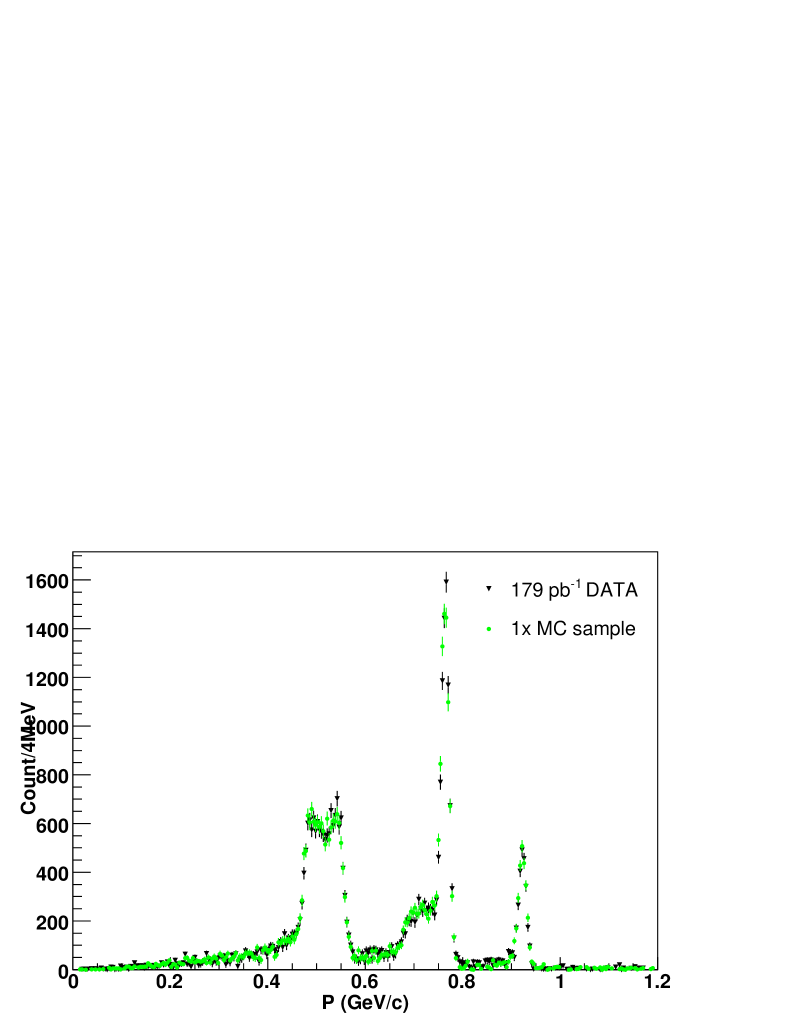
Figure 59: Comparison between MC and data at 4170 MeV for $D^{+}\rightarrow{K^{-}}\pi^{+}\pi^{+}$. Based on the momentum spectrum fit results an independent MC sample with the same statistics as the 178 pb${}^{-}1$ collected at 4170 MeV was generated using all the knowledge gained about ISR, angular distributions (see the App.) and cross sections.

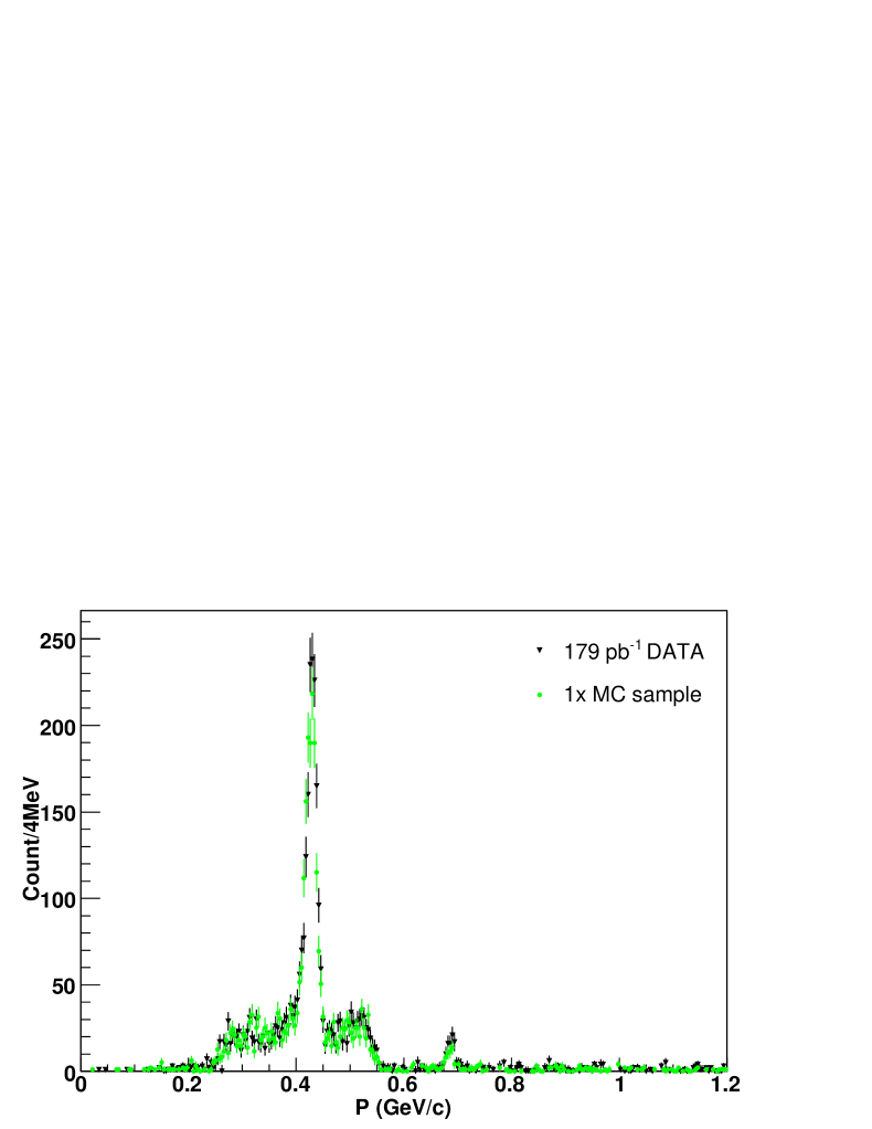
Figure 60: Comparison between MC and data, at 4170 MeV, for $D_{s}^{+}\rightarrow{\phi}\pi^{+}$. Based on the momentum spectrum fit results an independent MC sample with the same statistics as the 178 pb${}^{-}1$ collected at 4170 MeV was generated using all the knowledge gained about ISR, angular distributions (see the App.) and cross sections.

Since the fit for $D^{0}$ is independent of $D^{+}$, a ratio of these fit results, calculated for each event type, can be a good check of the method. The ratios for all event types and all energies are shown in Fig. 57. At all energies the ratios are in good agreement with what is expected (the solid horizontal lines). As a further check, a MC sample with the same statistics as the $178$ pb^-1 of data was generated. Figs. 58, 59, and 60 show the scaled momentum spectrum for $D^{0}\rightarrow{K^{-}}\pi^{+}$, $D^{+}\rightarrow{K^{-}}\pi^{+}\pi^{+}$, and $D^{+}\rightarrow\phi\pi^{+}$, respectively, for this sample overlaid with the data. The agreement is quite exceptional.

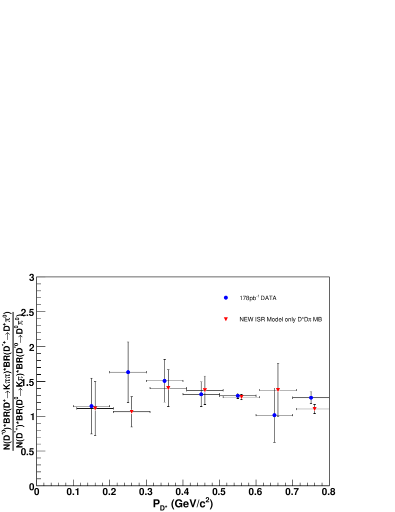
Figure 61: Ratio of $D^{*0}$ to $D^{*+}$ in 4170 MeV data and MC as a function of the reconstructed $D^{*}$ momentum. Both $D^{*}$ states are detected with the $\pi^{0}$ channel, with the subsequent decays $D^{0}\rightarrow{K^{-}}\pi^{+}$ and $D^{+}\rightarrow{K^{-}}\pi^{+}\pi^{+}$, respectively. The ratio is corrected for branching fractions, while efficiencies were assumed to be constant. The MC includes $D^{*}\bar{D}\pi$ multi-body and uses an updated ISR model that incorporates individual two-body cross sections as described in the text. The updated MC sample is in great agreement with the data at 4170 MeV.

For another confidence test of the procedure we used this one-times sample to verify the determination of the production ratios. Comparisons of $D^{*0}$ to $D^{*+}$ and $D^{0}$ to $D^{+}$ for the updated MC and data can be seen in Fig. 61 and Fig. 62. Overall, the previously observed discrepancies between the data and MC have been resolved with the use of a more accurate description of ISR in the MC.

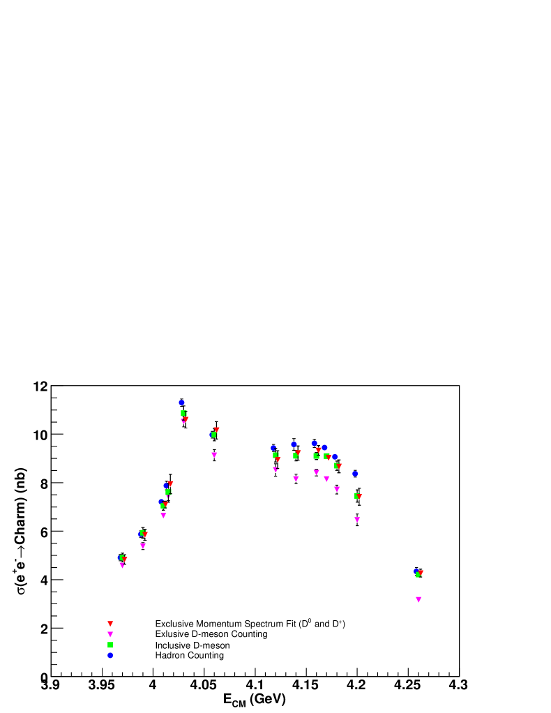
Figure 66: Plot of the total charm cross section as calculated by each of the three methods described in the text, in addition to the results from the momentum-spectrum fit. The reason for the discrepancy between the inclusive and exclusive method is due to the presence of multi-body background and ISR. These two effects are taken into account when a fit to the momentum spectrum is performed. There is good agreement between all three methods, the inclusive, the hadron counting and the momentum fits. The previous exclusive result (ignoring multi-body) is shown, in addition, for comparison.

The final measurements of multi-body production at energies above 4030 MeV are summarized in Table 27. The exclusive cross sections for all modes studied from the momentum-spectrum fits are shown in Tables 53 and 54, as well as in Figs. 63, 64, and 65. The total charm cross section for all three methods, as discussed in the text, are shown in Fig. 66. It should be noted, unless otherwise stated, that the weighted sum technique from Sect. 9 is used for the individual $D_{s}$ cross sections whose result is used in the determination of the total exclusive charm cross section, e.g. Fig. 66.

Table 27: The amount of multi-body present at energies above 4060 MeV obtained by fitting the sideband-subtracted momentum spectra for $D^{0}\rightarrow{K^{-}}\pi^{+}$ and $D^{+}\rightarrow{K^{-}}\pi^{+}\pi^{+}$ with the two-body MC representation of the various exclusive channels and a spin-averaged phase-space model MC representation of multi-body. There is no evidence for the $DD\pi$ final state at any energy. Only statistical errors are shown.

Ecm MeV	$\sigma(e^{+}e^{-}\rightarrow{D^{*}D\pi})$ nb	$\sigma(e^{+}e^{-}\rightarrow{D^{*}D^{*}\pi})$ nb
$4060$	$0.14\pm 0.09$	$-\pm-$
$4120$	$0.05\pm 0.08$	$-\pm-$
$4140$	$0.41\pm 0.09$	$-\pm-$
$4160$	$0.39\pm 0.06$	$-\pm-$
$4170$	$0.44\pm 0.01$	$-\pm-$
$4180$	$0.58\pm 0.09$	$-\pm-$
$4200$	$0.74\pm 0.13$	$-\pm-$
$4260$	$0.64\pm 0.09$	$0.32\pm 0.07$

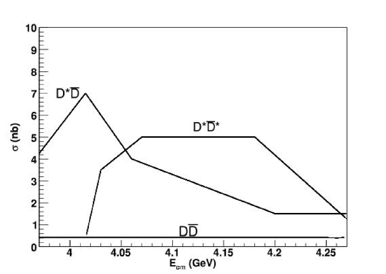
Figure 52: The two-body cross sections used in EVTGEN for $D\bar{D}$, $D^{*}\bar{D}$, and $D^{*}\bar{D}^{*}$ for the MC samples with improved treatment of ISR. A simple implementation of the cross sections were made using straight-line approximation for the real, Born-level, two-body, cross sections. The main assumption is that the shape of the cross section will be preserved after applying radiative corrections, that is the observed cross section shape is the same as the Born-level cross section shape.

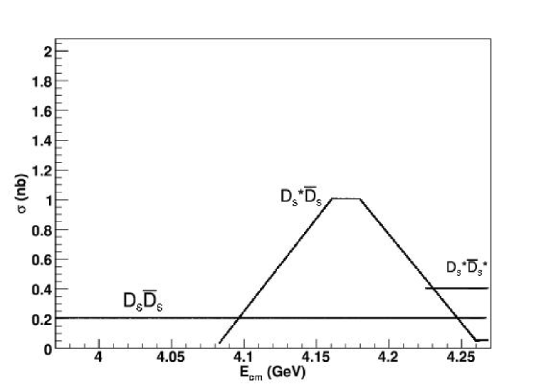
Figure 53: The two-body cross sections used in EVTGEN for $D_{s}\bar{D}_{s}$, $D_{s}^{*}\bar{D}_{s}$, and $D_{s}^{*}\bar{D}_{s}^{*}$ for the MC samples with improved treatment of ISR. A simple implementation of the cross sections were made using straight-line approximation for the real, Born-level, two-body cross sections. The main assumption is that the shape of the cross section will be preserved after applying radiative corrections, that is the observed cross section shape is the same as the Born-level cross section shape.

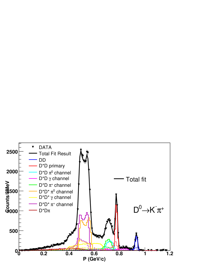
Figure 54: Sideband-subtracted momentum spectrum for $D^{0}\rightarrow{K^{-}}\pi^{+}$ at 4170 MeV. Data are shown as points with error bars which are fit to the improved ISR MC (histograms). The fit uses a spin-averaged phase-space model MC representation of $D^{*}\bar{D}\pi$, shown in dark red. The solid histograms correspond to $E_{\gamma}<1$ MeV (no ISR) while the dashed histograms correspond to $E_{\gamma}>1$ MeV (with ISR). The total fit result is shown by the solid black line ($\chi^{2}/NDF=248/132$).

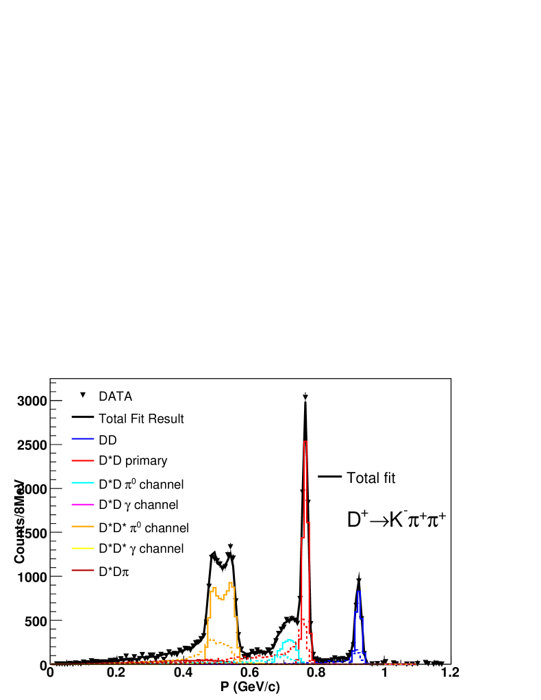
Figure 55: Sideband-subtracted momentum spectrum for $D^{+}\rightarrow{K^{-}}\pi^{+}\pi^{+}$ at 4170 MeV. Data are shown as points with error bars which are fit to the improved ISR MC, the histograms. The fit uses a spin-averaged phase-space model MC representation of $D^{*}D\pi$, shown in dark red. The solid histograms correspond to $E_{\gamma}<1$ MeV (no ISR) while the dashed histograms correspond to $E_{\gamma}>1$ MeV (with ISR). The total fit result is shown by the solid black line ($\chi^{2}/NDF=182/132$).

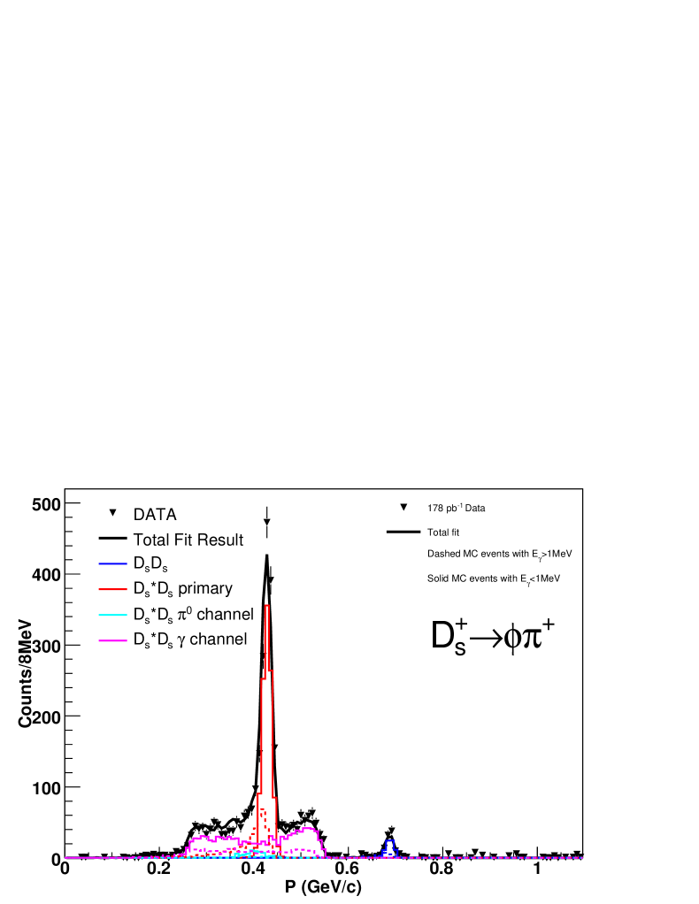
Figure 56: Sideband-subtracted momentum spectrum for $D_{s}^{+}\rightarrow\phi\pi^{+}$ at 4170 MeV. Data are shown as points with error bars which are fit to the improved ISR MC (histograms). The solid histograms correspond to $E_{\gamma}<1$ MeV (no ISR) while the dashed histograms correspond to $E_{\gamma}>1$ MeV (with ISR). The total fit result is shown by the solid black line ($\chi^{2}/NDF=165/124$).

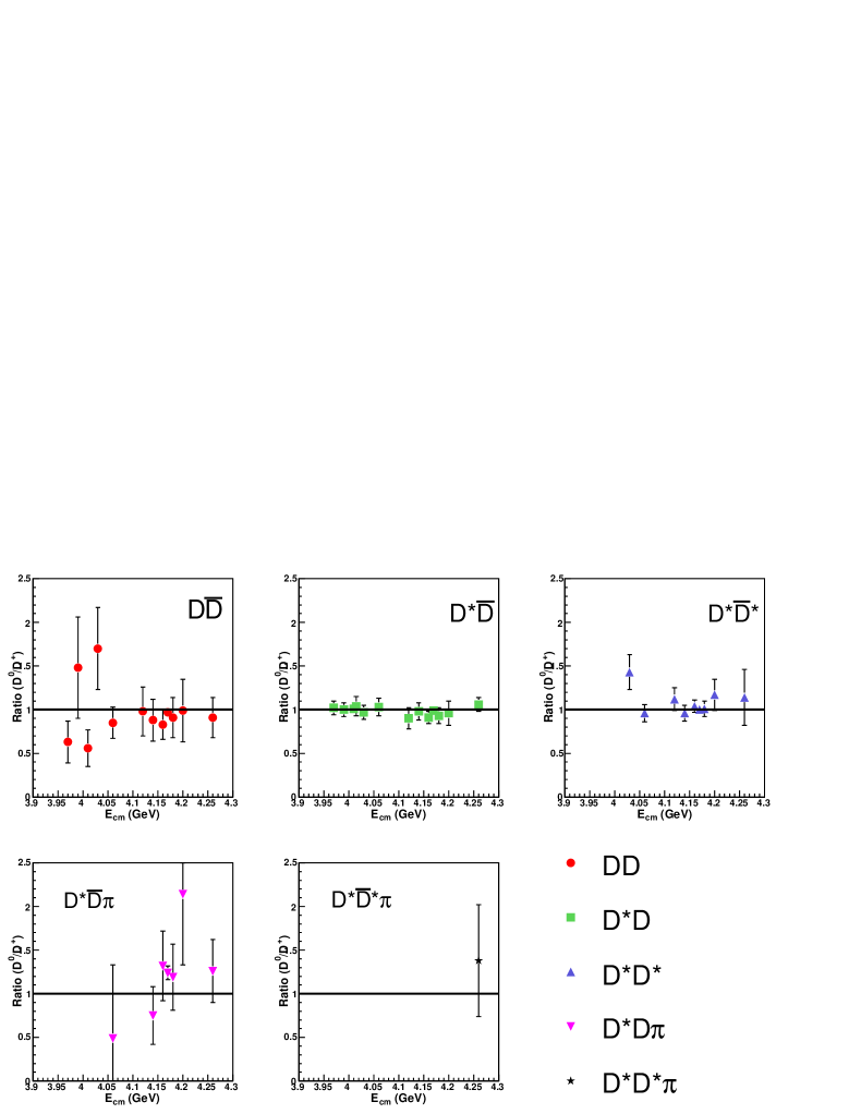
Figure 57: The ratio of the cross section results from the $D^{0}\rightarrow{K^{-}}\pi^{+}$ fit to the results from the $D^{+}\rightarrow{K^{-}}\pi^{+}\pi^{+}$ fit. Since the fits are independent, the agreement in the ratios demonstrates the reliability of the fitting procedure in extracting the mode-by-mode cross sections. The ratio, in all cases, should be one, indicated by the solid black line. All event types are in good agreement with what is expected.

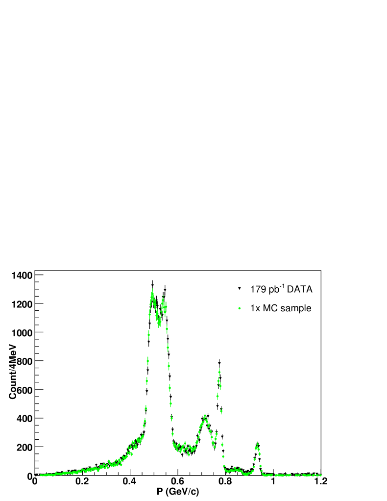
Figure 58: Comparison between MC and data at 4170 MeV for $D^{0}\rightarrow{K^{-}}\pi^{+}$. Based on the momentum spectra fit results, an indepedent MC sample with the same statistics as the 178 pb^-1 collected at 4170 MeV was generated using all the knowledge gained about ISR, angular distributions (see the App.) and cross sections.

Figure 62: Ratio of the number of $D^{0}$ to $D^{+}$ as a function of reconstructed $D$ momentum at $E_{{\rm{cm}}}=4170$ MeV. The ratio is corrected for branching fractions, while efficiencies were assumed to be constant. The MC includes $D^{*}\bar{D}\pi$ multi-body and uses an updated ISR model that incorporates individual two-body cross sections as described in the text. The updated MC sample is in great agreement with the data at 4170 MeV.

Figure 63: Observed cross sections for $e^{+}e^{-}\rightarrow{D\bar{D}}$, $D^{*}\bar{D}$ and $D^{*}\bar{D}^{*}$ as a function of center-of-mass energy. They are determined by fitting the momentum spectrum for $D^{0}\rightarrow{K^{-}}\pi^{+}$ and $D^{+}\rightarrow{K^{-}}\pi^{+}\pi^{+}$ with the updated ISR MC. Systematic errors are not included.

Figure 64: Observed cross sections for $e^{+}e^{-}\rightarrow{D_{s}\bar{D}_{s}}$, $D_{s}^{*}\bar{D}_{s}$ and $D_{s}^{*}\bar{D}_{s}^{*}$ as a function of center-of-mass energy. They are determined by fitting the momentum spectrum for $D_{s}^{+}\rightarrow\phi\pi^{+}$ with the updated ISR model MC. A branching fraction of 3.6% was also used in the determination of the cross section. Systematic errors are not included.

Figure 65: Observed cross sections for $e^{+}e^{-}\rightarrow{D^{*}\bar{D}\pi}$ and $D^{*}\bar{D}^{*}\pi$ as a function of center-of-mass energy. They are determined by fitting the momentum spectrum for $D^{0}\rightarrow{K^{-}}\pi^{+}$ and $D^{+}\rightarrow{K^{-}}\pi^{+}\pi^{+}$ with the updated ISR model MC. The multi-body contribution was modeled in MC using spin-averaged phase space. Systematic errors are not included.

11 Momentum Spectrum and Multi-Body Cross-Check

Using the improved 178 pb^-1 MC sample that was generated to check the neutral-to-charged $D$-meson ratio, one can check the momentum-spectrum fit procedure. The momentum-spectrum fit results for $D^{0}\rightarrow{K^{-}}\pi^{+}$, $D^{0}\rightarrow{K^{-}}\pi^{+}\pi^{+}$, and $D_{s}^{+}\rightarrow{\phi}\pi^{+}$ are shown in Figs. 67, 68, and 69 respectively. The comparison between what was generated and what is obtained from the fit is shown in Table 28. The returned fit results are in very good agreement with what was used to generate the sample.

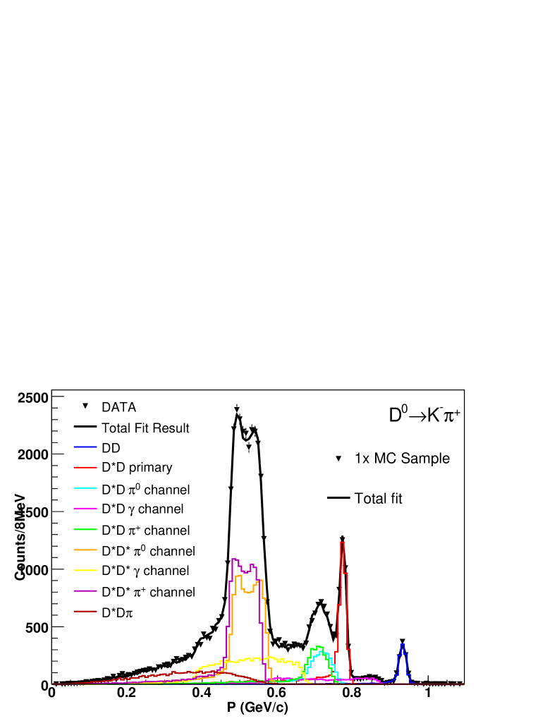
Figure 67: Momentum-spectrum fit for the improved 178 pb^-1 MC sample for $D^{0}\rightarrow{K^{-}}\pi^{+}$. The MC sample was treated just as the data and used as a cross-check of the momentum-spectrum fit procedure.

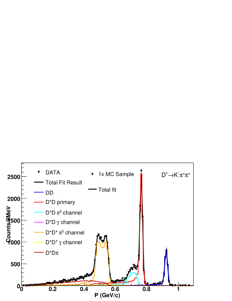
Figure 68: Momentum-spectrum fit for the improved 178 pb^-1 MC sample for $D^{+}\rightarrow{K^{-}}\pi^{+}\pi^{+}$. The MC sample was treated just as the data and used as a cross-check of the momentum-spectrum fit procedure.

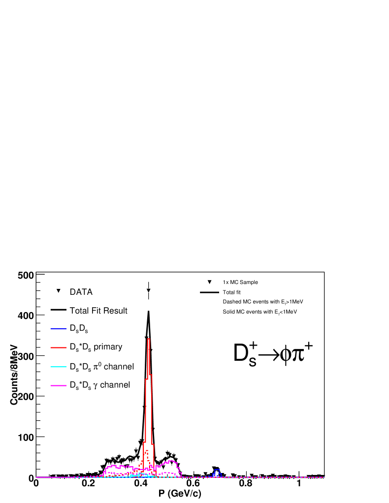
Figure 69: Momentum-spectrum fit for the improved 178 pb^-1 MC sample for $D_{s}^{+}\rightarrow{\phi}\pi^{+}$. The MC sample was treated just as the data and used as a cross-check of the momentum-spectrum fit procedure.

Table 28: Results of the momentum-spectrum fit of the improved 178 pb^-1 MC sample. The agreement between the fitted and the generated values is very reasonable.

Parameter	Fitted Value (nb)	Generated Value (nb)	Difference
$D\bar{D}$	$0.319\pm 0.008$	$0.331$	$-1.5\sigma$
$D^{*}\bar{D}$	$2.392\pm 0.08$	$2.392$	$-0.1\sigma$
$D^{*}\bar{D}^{*}$	$4.553\pm 0.038$	$4.508$	$1.2\sigma$
$D^{*}\bar{D}\pi$	$0.766\pm 0.018$	$0.780$	$-0.8\sigma$
$D_{s}\bar{D}_{s}$	$0.036\pm 0.005$	$0.040$	$-0.8\sigma$
$D^{*}_{s}\bar{D}_{s}$	$1.039\pm 0.028$	$0.994$	$1.6\sigma$

As an additional check on the multi-body contributions at 4170 MeV and 4260 MeV, the two energies where either a large amount of data existed or a large amount of multi-body is present, one can fit the missing-mass spectrum to obtain the cross section for multi-body. The fit results for $D^{*0}\rightarrow{D^{0}\pi^{0}}$ with $D^{0}\rightarrow{K^{-}}\pi^{+}$, and $D^{*+}\rightarrow{D^{+}\pi^{0}}$ with $D^{+}\rightarrow{K^{-}}\pi^{+}\pi^{+}$ plus an additional charged pion at 4170 MeV are shown in Figs. 70 and 71, respectively. The fit results for $D^{*0}\rightarrow{D^{0}\pi^{0}}$ with $D^{0}\rightarrow{K^{-}}\pi^{+}$, $D^{0}\rightarrow{K^{-}}\pi^{+}\pi^{0}$, or $D^{0}\rightarrow{K^{-}}\pi^{+}\pi^{+}\pi^{-}$ plus an additional charged pion at 4260 MeV is shown in Fig. 72. Using a spin-averaged phase-space model MC sample to determine the corresponding efficiencies the cross sections can be determined. The results from this method are shown, along with the momentum-spectrum fit results, in Table 29. The agreement between these two different methods supplies more confidence in the results that are being presented.

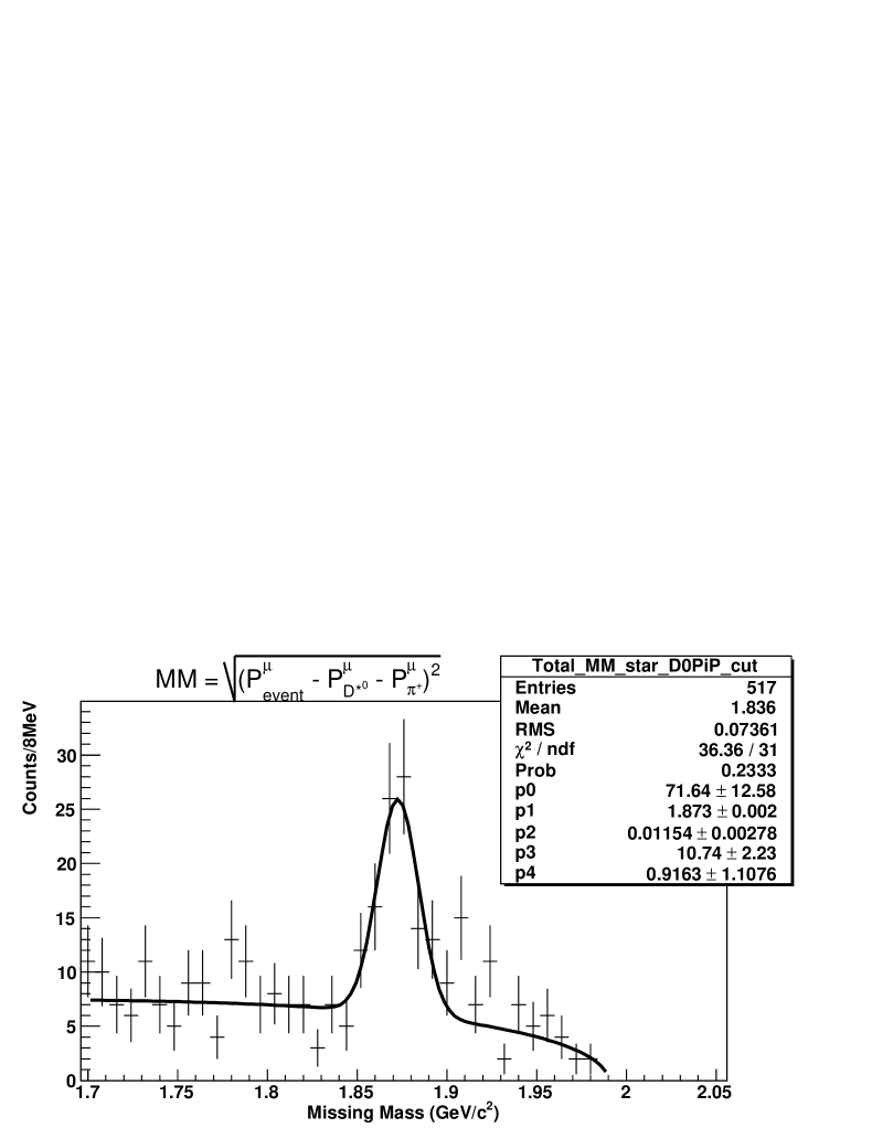
Figure 70: Missing-mass spectrum using $D^{0}\rightarrow{K^{-}}\pi^{+}$ at 4170 MeV. The fit function consists of a Gaussian and an Argus function.

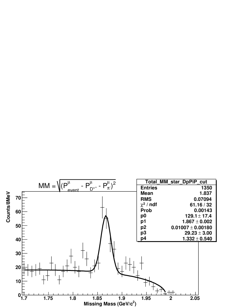
Figure 71: Missing-mass spectrum using $D^{+}\rightarrow{K^{-}}\pi^{+}\pi^{+}$ at 4170 MeV. The fit function consists of a Gaussian and an Argus function.

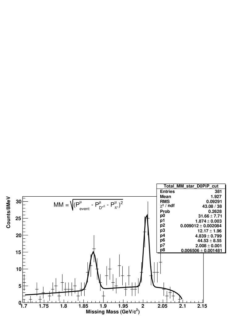
Figure 72: Missing-mass spectrum using $D^{0}\rightarrow{K^{-}}\pi^{+}$, $D^{0}\rightarrow{K^{-}}\pi^{+}\pi^{0}$, and $D^{0}\rightarrow{K^{-}}\pi^{+}\pi^{+}\pi^{-}$ at 4260 MeV. The fit function consists of two Gaussians, one for each peak, and an Argus function.

Table 29: Comparison between the momentum-spectrum results and fits to the missing-mass spectrum for multi-body at 4170 MeV and 4260 MeV. The agreement between the two different methods instills confidence on our handling of multi-body events.

Parameter	Energy (MeV)	Missing-Mass	Momentum-Spectrum
		Value (nb)	Value (nb)
$D^{*}\bar{D}\pi(D^{*0})$	$4170$	$0.34\pm 0.06$	$0.44\pm 0.01$
$D^{*}\bar{D}\pi(D^{*+})$	$4170$	$0.42\pm 0.06$	$0.44\pm 0.01$
$D^{*}\bar{D}\pi(D^{*0})$	$4260$	$0.62\pm 0.16$	$0.64\pm 0.09$
$D^{*}\bar{D}^{*}\pi(D^{*0})$	$4260$	$0.23\pm 0.05$	$0.32\pm 0.07$

Chapter SYSTEMATICS

12 Exclusive Cross Sections via Momentum
Spectrum Fits

Using the published CLEO-c 56 pb^-1 analysis [45, 46], at all energies we apply a 0.7%, 0.3%, and 1.3% systematic for tracking, pion PID, and kaon PID respectively. In addition, we apply a 1% systematic to the luminosity [58]. Also, the error on the respective branching ratios are 3.1% for $D^{0}\rightarrow{K^{-}}\pi^{+}$, 3.9% for $D^{+}\rightarrow{K^{-}}\pi^{+}\pi^{+}$ [45, 46], 0.7% for $D^{*+}\rightarrow{D^{0}\pi^{+}}$ [2] and the respective errors associated with $D_{s}$ decays [2, 44].

Besides the aforementioned systematic errors, the additional area where systematic errors will be present is in the cross section shape assumed in EVTGEN [57]. The systematic error resulting from the shape of the cross section was determined by adjusting the two-body exclusive cross sections from their nominal shapes (Fig. 52 and Fig. 53). The adjustments were determined by the existing data points as well as taking some extremes to understand the effect of the shape of the cross section assumed in EVTGEN. The systematic errors were investigated on the large data-set at 4170 MeV since statistical errors are minimized. Lastly, since an adjustment to the shape of single cross section can effect the other cross sections in the fit, the total systematic error for an individual cross section is determined by adding in quadrature all cross section effects.

12.1 $D\bar{D}$

Two adjustments were investigated in regards to the shape of the cross section. First, a step was added starting at 4015 MeV and extending to 4120 MeV where the cross section was doubled. Since the cross section in this range is larger, as compared to the nominal assumption of a flat cross section across all energies, the probability distribution will reflect this change. Events which radiate a photon for this energy range are now more probable and the fit results for this assumed cross section will be larger as compared to the nominal assumption. The next adjustment investigated is a decreasing cross section as a function of increasing energy, the slope is 2 nb/GeV. Following similar logic as before, if the cross section at lower energies is larger, as compared to the cross section at 4170 MeV and the nominal flat cross section then the fit result will report a larger result for the $D\bar{D}$ and $D_{s}\bar{D}_{s}$ cross sections as is shown in Table 30. Similar results are obtained for a cross section that is smaller at lower energies, as compared to the cross section at 4170 MeV. Since increasing and decreasing the cross sections, at 2 nb/GeV, are extreme adjustments, whereas the box is a conservative adjustment, the two are averaged and used in the determination of the systematic errors. The former is considered extreme because the data does not suggest this type of behavior.

Table 30: Relative systematic errors for adjustments to the $D\bar{D}$ cross section.

Event Type	Box 4015-4120 MeV	Slope ($m=2$ nb/GeV)	Average
$D\bar{D}$	$+2.1\%$	$+4.2\%$	$+3.2\%$
$D^{*}\bar{D}$	$-0.5\%$	$-0.5\%$	$-0.5\%$
$D^{*}\bar{D}^{*}$	$+0.1\%$	$+0.1\%$	$+0.1\%$
$D^{*}\bar{D}\pi$	$+0.3\%$	$+0.2\%$	$+0.3\%$

12.2 $D^{*}\bar{D}$

Two adjustments were investigated in regards to the shape of the cross section. First, the cross section was adjusted to take out the kink at 4060 MeV allowing the cross section to decrease constantly and continuously from 4015-4170 MeV. Since the cross section is increasing one would expect the fit result to reflect this change and increase. However, since there is an overlap of both $D\bar{D}$ and $D^{*}\bar{D}^{*}$, the simple explanation is no longer straight forward. The next adjustment was to assume a flat cross section until 4060 MeV at which energy the cross section then increased to 4015 MeV. This assumption results in a poor fit to the momentum spectrum, most notable in the $D^{+}\rightarrow{K^{-}}\pi^{+}\pi^{+}$ distribution as seen in Fig. 73. Therefore, because the latter assumption produces a poor fit, systematic errors of the former are used. Since there is overlap between the various two-body states present at this energy changes to the $D^{*}\bar{D}$ effects to the other cross sections result which are evident in Table 31.

Table 31: Relative systematic errors for $D^{*}\bar{D}$.

Event Type	Continuous Decrease From 4015 MeV	Flat to 4060 MeV
$D\bar{D}$	$+0.6\%$	$+0.8\%$
$D^{*}\bar{D}$	$-1.1\%$	$-5.2\%$
$D^{*}\bar{D}^{*}$	$+0.4\%$	$+3.0\%$
$D^{*}\bar{D}\pi$	$+3.0\%$	$+2.0\%$

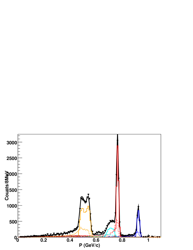
Figure 73: The fit result after adjusting the $D^{*}\bar{D}$ cross section from its nominal value to one that is flat between 4060-4170 MeV. The change results in a poor fit most notable at 600 MeV/$c$.

12.3 $D^{*}\bar{D}^{*}$

For these events we investigated changes to the shape of the cross section in addition to changes in the respective helicity amplitudes. First, the cross section for $D^{*}\bar{D}^{*}$ was adjusted such as to add a dip in the plateau region of the nominal cross section. In a similar situation as $D^{*}\bar{D}$, the addition of other possible two-body states along with the addition of multi-body a simple expectation is difficult to ascertain. Another adjustment was to remove the kink at 4030 MeV and to allow the cross section to decrease continuously to zero at 4060 MeV. The effects of both adjustments on the $D^{*}\bar{D}^{*}$ along with the other cross sections is shown in Table 32.

Table 32: Relative systematic errors for adjustments in the shape of the cross section for $D^{*}\bar{D}^{*}$.

Event Type	Dip	Decrease to Zero at 4070 MeV
$D\bar{D}$	$-$	$-$
$D^{*}\bar{D}$	$-$	$+0.2\%$
$D^{*}\bar{D}^{*}$	$+2.4\%$	$-2.4\%$
$D^{*}\bar{D}\pi$	$-1.5\%$	$+9.1\%$

The helicity amplitude affect the angular distributions of the $D^{*}\bar{D}^{*}$ final state and therefore has an effect of the resulting daughter $D$ (See Appendix for a discussion of angular distributions). This shows up, most notably, in the momentum spectrum resulting from the $\pi$ decay channel, between 500-600 MeV/$c$. Taking an extreme case we adjusted the coefficient in front of the $\cos$ for the angle between the $D$ in the rest frame of the $D^{*}$ with respect to the momentum of $D^{*}$ in the lab from its nominal value of 0.8 to 2.0. The result is shown in Fig. 74 which clearly shows that such a change results in a bad fit. The effect on the cross sections is shown in Table 33.

Table 33: Relative systematic errors for adjustments in the helicity amplitudes for $D^{*}\bar{D}^{*}$.

Event Type	Angle ($\alpha^{{}^{\prime}}=2$)
$D\bar{D}$	$-$
$D^{*}\bar{D}$	$+0.3\%$
$D^{*}\bar{D}^{*}$	$-1.0\%$
$D^{*}\bar{D}\pi$	$+6.0\%$

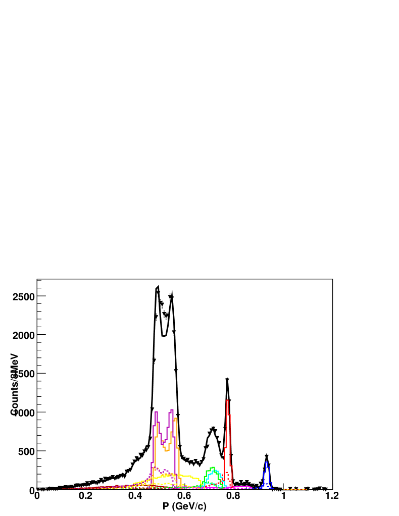
Figure 74: The fit result after adjusting the angle between the $D$ in the rest frame of the $D^{*}$ with respect to the momentum of $D^{*}$ in the lab from its nominal value of 0.8 to 2.0. The fit is poor most notably between 500-600 MeV/$c$.

12.4 $D^{*}\bar{D}\pi$

Rather than assuming a flat cross section as a function of energy, an adjustment that allows the cross section to increase as the energy increases. Since the cross section is now smaller at lower energies, as compared to the cross section at 4170 MeV, the fit result will return a larger result. Because the momentum range of the multi-body event is large, between 0-500 MeV/$c$, such a change in the cross section will result in modest changes to the fit results which are shown in Table 34.

Table 34: Relative systematic errors for adjustments made to the shape of the cross section for $D^{*}\bar{D}\pi$.

Event Type	Increasing Slope ($m=4$ nb/GeV)
$D\bar{D}$	$-$
$D^{*}\bar{D}$	$-$
$D^{*}\bar{D}^{*}$	$-$
$D^{*}\bar{D}\pi$	$+2.7\%$

12.5 $D^{*}\bar{D}^{*}\pi$

Since there is only one data point for $D^{*}\bar{D}^{*}\pi$ a systematic of 25% is assigned.

12.6 Total Systematic Errors: Exclusive Momentum Fit Method

The total systematic errors for the exclusive cross sections by fitting the momentum spectrum are shown in Table 35.

Table 35: Total relative systematic errors for the exclusive momentum fit method.

Event Type	Total
$D\bar{D}$	$4.5\%$
$D^{*}\bar{D}$	$3.4\%$
$D^{*}\bar{D}^{*}$	$4.7\%$
$D^{*}\bar{D}\pi$	$12\%$
$D^{*}\bar{D}^{*}\pi$	$25\%$

12.7 Systematic Errors: $D_{s}\bar{D}_{s}$, $D_{s}^{*}\bar{D}_{s}$ and $D_{s}^{*}\bar{D}_{s}^{*}$

For $D_{s}\bar{D}_{s}$, $D_{s}^{*}\bar{D}_{s}$ and $D_{s}^{*}\bar{D}_{s}^{*}$, a weighted sum technique is used to combine the eight $D_{s}$ decay modes and obtain the cross sections. This technique was used to minimize the error, both statistical and systematic. Since multi-body type events involving a $D_{s}$-meson are not expected by isospin which was confirmed by not observing evidence of multi-body events in the momentum spectra of $D_{s}\rightarrow\phi\pi^{+}$ at any of energies, the technique described in Sect. 9 is used. Besides the errors in regards to the branching fractions, shown in Table 37, are errors resulting from the technique. It should be mentioned that because of the recently updated $D_{s}$ branching fractions [44] the weights used in the calculation are not optimal because they were determined using the PDG 2005 [2] values. However, the changes in the branching fractions have a minor, if no, effect on the final result by virtue of the technique. To demonstrate this we look at the results for $D_{s}$ at 4170 MeV. By comparing both the individual mode results and the weighted sum result, Table 36, one sees that the agreement between them is quite good and the updated branching fractions reduce the associated systematic error without effecting the quoted value for the $D_{s}$ cross sections stated in Sect. 9.

Table 36: A comparison between the $D_{s}^{*}D_{s}$ cross sections at 4170 MeV determined by individual modes using the recently updated branching fractions [44] to that of the weighted sum technique using branching fractions based on [2]. The agreement between the individual modes and the weighted sum stresses the fact that the result from the weighted sum is not effected by the changes in the branching fractions. The only effect of the updated branching fractions is to decrease the systematic errors.

Mode	Cross Section (nb)
$K_{s}K^{+}$	$0.85\pm 0.05$
$\pi^{+}\eta$	$0.99\pm 0.05$
$\pi^{+}\eta^{{}^{\prime}}$	$0.90\pm 0.04$
$\pi^{+}\phi$	$0.96\pm 0.03$
Weighted Sum	$0.92\pm 0.01$

Table 37: The $D_{s}$ branching fractions including the updated branching fractions, in $10^{-2}$.

Modes	Branching Fraction
$\phi\pi^{+}$, 10 MeV cut on the Invariant $\phi\rightarrow{K}^{+}K^{-}$ Mass [44]	$1.98\pm 0.15$
$K^{*0}K^{+},K^{*0}\rightarrow{K^{-}\pi^{-}}$ [2]	$2.2\pm 0.6$
$\eta\pi^{+},\eta\rightarrow{\gamma\gamma}$ [2, 44]	$0.58\pm 0.07$
$\eta\rho^{+},\eta\rightarrow{\gamma\gamma},\rho^{+}\rightarrow{\pi^{+}\pi^{0}}$ [2]	$4.3\pm 1.2$
$\eta^{{}^{\prime}}\pi^{+},\eta^{{}^{\prime}}\rightarrow{\pi^{+}\pi^{-}\eta},\eta\rightarrow{\gamma\gamma}$ [2, 44]	$0.7\pm 0.1$
$\eta^{{}^{\prime}}\rho^{+},\eta^{{}^{\prime}}\rightarrow{\pi^{+}\pi^{-}\eta},\eta\rightarrow{\gamma\gamma},\rho^{+}\rightarrow{\pi^{+}\pi^{0}}$ [2]	$1.8\pm 0.5$
$\phi\rho^{+},\phi\rightarrow{K^{+}K^{-}},\rho^{+}\rightarrow{\pi^{+}\pi^{0}}$ [2]	$3.4\pm 1.2$
$K_{s}K^{+},K_{s}\rightarrow{\pi^{+}\pi^{-}}$ [2, 44]	$1.0\pm 0.07$

The selection criteria, ${\rm{M_{bc}}}$ and $\Delta{\rm{E}}$, for the various exclusive cross sections result in added systematic errors. Having adjusted the $\Delta{\rm{E}}$ cut window by 10 MeV the cross sections for $D_{s}\bar{D}_{s}$ changed by a maximum of 3% and therefore 3% is applied to these cross sections at all energies. Next, by adjusting the ${\rm{M_{bc}}}$ cut window by 10 MeV for $D_{s}^{*+}{D}_{s}^{-}$ the cross sections changed by 2.5% and therefore 2.5% is applied to these cross sections at all energies. The charge in ${\rm{M_{bc}}}$ was asymmetric because the photon decay mode is included and allows for $D_{s}$ to be spread out over a wide range of momenta. Lastly, by adjusting ${\rm{M_{bc}}}$ by 30 MeV for $D_{s}^{*+}\bar{D}_{s}^{*-}$ the result changed by 5% therefore 5% is applied to these cross sections at all energies. The table of systematics for the exclusive method is shown in Table 38.

Table 38: Total relative systematic errors for the $D_{s}$ cross sections.

Event Type	Total
$D_{s}\bar{D}_{s}$	$5.6\%$
$D_{s}^{*}\bar{D}_{s}$	$5.3\%$
$D_{s}^{*}\bar{D}_{s}^{*}$	$6.8\%$

13 Inclusive $D$ Method

Using the published CLEO-c 56 pb^-1 analysis [45, 46], at all energies we apply a 0.7%, 0.3%, and 1.3% systematic for tracking, pion PID, and kaon PID respectively. In addition, we apply a 1% systematic to the luminosity [58]. The largest systematic in regards to this method is assigned to the fit function and the yields obtained by a gaussian plus a polynomial of degree two. Changing the background function to a linear function causes a 2% shift, which is the largest, is seen in the yields of $D^{0}$ and $D^{+}$. At energies above the $D_{s}\bar{D}_{s}^{*}$ threshold a 7% shift, which is largest, is seen in the $D_{s}$ yields and 2% at all energies below threshold. In all cases, except 4170 MeV, the change in yields is $<1\sigma$. Lastly, the error on the respective branching ratios are 3.1% for $D^{0}\rightarrow{K^{-}}\pi^{+}$, 3.9% for $D^{+}\rightarrow{K^{-}}\pi^{+}\pi^{+}$ [45, 46] and 6.4% for $D_{s}^{+}\rightarrow{K^{-}}K^{+}\pi^{+}$ [44]. Therefore, we quote a systematic of 4.3% for $D^{0}$ and 5.1% for $D^{+}$ at all energies. For $D_{s}$ an extra systematic error of 4%, associated with the selection criteria, is applied. The determination of the latter systematic error was taken from the investigation of the exclusive cross sections for $D_{s}^{*+}{D}_{s}^{-}$ and $D_{s}^{+}{D}_{s}^{-}$. Therefore, $D_{s}$ is quoted with a systematic error of 8.6% for energies below 4100 MeV and 10.8% for those above. The systematic error associated with the branching fractions, as well as the PID and tracking, should be improved in the near future with the updated $D$ and $D_{s}$ branching fractions.

14 Hadron-Counting Method

Since the method that was used here is identical to method used to determine the cross section of $e^{+}e^{-}\rightarrow\psi(3770)\rightarrow{hadrons}$ at $E_{\rm{cm}}=3770$ MeV [49, 50, 51], most of the systematics will be identical. One difference that was investigated was the systematic that is associated with the hadronic event selection criteria, since this could vary with energy. By applying tighter cuts, THAD [49, 51], the maximum change in the cross at any energy was 4.5% and so is taken as the hadronic event criteria systematic for all energies. In a similar fashion, as in the reference [49, 50, 51], a conservative error, to account for the interference with the continuum and because they are based on theoretical calculation, of 25% will be associated with $\psi(2S)$, $J/\psi$, and $\psi(3770)$ subtraction at each energy. Since the cross section varies for these backgrounds, so does the associated error. Errors which are common between the energies are shown in Table 39, whereas the energy dependent errors are shown in Table 40, including the total.

Table 39: Summary of various systematic errors that are common amongst the scan energies for the hadron counting method.

Source of error	relative errors in $10^{-2}$
QED/Two-Photons subtractions/suppressions	0.3
BeamGas/Wall/Cosmic subtraction	0.5
Track quality cuts	0.5
Luminosity	1.0
Continuum scaling	2.1
Hadronic event selection criteria	4.5
Total common systematic error	5.1

Table 40: Summary of the energy dependent systematic errors, in $10^{-2}$, for the hadron counting method.

Energy (MeV)	$J/\psi$	$\psi(2S)$	$\psi(3770)$	Total relative Systematic Errors
3970	3.1	1.30	0.44	6.1
3990	2.3	1.13	0.34	5.7
4010	1.8	0.88	0.25	5.5
4015	1.6	0.80	0.23	5.4
4030	1.1	0.54	0.14	5.2
4060	1.1	0.61	0.15	5.3
4120	0.99	0.53	0.12	5.2
4140	0.91	0.51	0.12	5.2
4160	0.89	0.48	0.10	5.2
4170	0.88	0.49	0.10	5.2
4180	0.88	0.49	0.11	5.2
4200	0.91	0.50	0.12	5.2
4260	1.53	0.80	0.19	5.4

Chapter Radiative Corrections

The Born or tree-level cross section is obtained by correcting the observed cross sections for the effects of initial-state radiation (ISR). In high-energy electron-positron annihilation experiments, the incoming particles can radiate. The radiated photons can be quite energetic, thereby changing the effective center-of-mass collision energy appreciably. Therefore, the annihilation energy is not always twice the beam energy and the observed cross sections obtained in the experiment correspond not to a single energy point but instead to a range of energies.

The needed correction factors were calculated using two alternate procedures. First, by following the method laid out by E.A. Kuraev and V.S. Fadin [56] which states that the observed cross section $\sigma_{obs}(s)$ at any energy $\sqrt{s}$ can be written as

$$\sigma_{obs}(s)=\int\limits_{0}^{1}dk\cdot f(k,s)\sigma_{B}(s_{eff}),$$ (38)

where $\sigma_{B}$ is the Born cross section as a function of the effective center-of-mass energy squared and $s_{eff}=s(1-x)$, with $E_{\gamma}=xE_{\rm{beam}}$. The function, $f(x,s)$ is defined as follows:

$$f(x,s)=tx^{t-1}[1+\frac{\alpha}{\pi}(\frac{\pi^{2}}{3}-\frac{1}{2})+\frac{3}{4}t-\frac{t^{2}}{24}(\frac{1}{3}\ln\frac{s}{m_{e}^{2}}+2\pi^{2}-\frac{37}{4})]-t(1-\frac{x}{2})$$

$$+\frac{t^{2}}{8}[4(2-x)\ln\frac{1}{x}-\frac{1+3(1-x)^{2}}{x}\ln(1-x)-6+x],$$ (39)

where $t=\frac{2\alpha}{\pi}[\ln(\frac{s}{m_{e}^{2}})-1]$. Eq.  is only used to first order in $t$.

The other method, by G. Bonneau and F. Martin [59], states that the observed cross section can be written in terms of the Born cross section as follows:

$$\sigma_{\rm{obs}}=\sigma_{B}[1+\frac{2\alpha}{\pi}\{(2\ln\frac{2E}{m_{e}}-1)(\ln{x_{min}}+\frac{13}{12}+$$

$$\int^{1}_{x_{min}}\frac{dx}{x}(1-x+\frac{x^{2}}{2})\frac{\sigma(s(1-x))}{\sigma{(s)}})-\frac{17}{36}+\frac{\pi^{2}}{6}\}].$$ (40)

Since the integral is infrared divergent, the $\ln{x_{min}}$ in Eq.  corresponds to the low-energy cutoff.

The only difference between the two methods is that G. Bonneau and F. Martin include the vacuum polarization for the electron, i.e. the electron bubble:

$$\delta_{vp}=\frac{2\alpha}{\pi}[-\frac{5}{9}+\frac{1}{3}\ln\frac{s}{m_{e}^{2}}].$$ (41)

We confirmed this by subtracting Eq. 41 from Eq.  and applying to the simple test of a constant cross section as a function of center-of-mass energy.

Note that Eqs.  and are dependent on the tree-level cross section, not only at $s$, but at all energies below $s$. Therefore, the ISR correction relies on a theoretical model or on already-radiatively-corrected experimental data to describe the shape of the cross section at all relevant energies.

It was decided to approach determining the shape of the cross section at lower energies with two different methods and to test on two different sets of already-radiatively-corrected data. The two data sets are from $R$ measurements in the region above $c\bar{c}$ threshold made by BES [18] and Crystal Ball (CB) [60]. The two shape methods were a simple linear-interpolation procedure applied to each data set, and a fit consisting of a sum of Breit-Wigners. Each of these methods was applied to the data sets after the $uds$ background had been subtracted using $\sigma_{uds}\sim\frac{196~{}{\rm{GeV^{2}}}~{}{\rm{nb}}}{s}$.

The results after radiatively correcting the inclusive cross section are shown in Fig. 75. The difference in the corrected cross section between the two shape-determining methods is mainly due to the interpolation method being influenced by the “jitteriness” of the data. Since this method is a simple linear interpolation, the fluctuations in the data play an important role, especially in the region nearest to the point that is to be corrected. Even so, the agreement is quite good, as seen in Table 41. The agreement between the two radiative correction methods, BM and KF, is excellent, giving us confidence that both have been implemented correctly. The difference between the methods is taken to be the systematic error for the ISR correction, which gives a 4% systematic error on the correction factor for all energies. Since all the methods are in good agreement, the KF interpolation method on the CB data has been chosen for the nominal results. The corrected inclusive cross section for the energies investigated are shown in Table 42 and graphically in Fig. 76.

A measurement of $R_{{\rm{charm}}}$, sometimes referred to as $R_{D}$, can be made by dividing $\sigma_{{\rm{charm}}}$ by the QED tree-level cross section for muon pair production, Eq. 2. In addition to $R_{{\rm{charm}}}$, one needs to determine $R_{uds}$, where $u$,$d$, and $s$ refer to the contribution of the light quarks to the measurement of R. By fitting $e^{+}e^{-}\rightarrow{{hadrons}}$, Fig. 4, between 3.2 and 3.72 GeV, with a $\frac{1}{s}$ function we arrive at $R_{uds}=2.285\pm 0.03$. The value of $R$ is then computed as the sum of these contributions:

$$R=R_{uds}+R_{{\rm{charm}}}$$ (42)

the results for $R$ are shown in Table 43 and graphically in Fig. 77.

Table 41: The radiative correction factors used in obtaining the tree-level total charm cross section results. The two different shape methods, calculation procedures, and the two data sets used are shown. Note that the corrected cross sections include the correction due to the vacuum polarization, as defined in Eq. 41 as well as the bubbles due to $\mu$ and $\tau$ leptons.

Ecm (MeV)	BESKF	BESBM	BESKF	CBKF	CBBM	CBKF
	Inter.	Inter.	FIt	Inter	Inter	Fit
3970	0.84	0.82	0.86	0.83	0.81	0.85
3990	0.92	0.94	0.85	0.86	0.86	0.83
4010	0.85	0.84	0.83	0.82	0.80	0.82
4015	0.82	0.79	0.83	0.85	0.84	0.82
4030	0.84	0.82	0.83	0.83	0.82	0.83
4060	0.86	0.86	0.86	0.92	0.93	0.89
4120	0.93	0.94	0.95	0.93	0.93	0.92
4140	0.98	1.00	0.93	0.95	0.96	0.91
4160	0.95	0.96	0.91	0.96	0.97	0.93
4170	0.94	0.96	0.92	0.95	0.96	0.92
4180	0.95	0.96	0.94	0.93	0.94	0.97
4200	1.00	1.02	1.02	1.02	1.05	1.02
4260	1.17	1.22	1.16	1.13	1.17	1.13

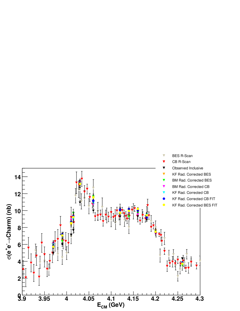
Figure 75: The radiatively corrected inclusive cross sections using all methods are compared to the BES and CB $uds$-subtracted $R$ data. Note that the corrected cross sections (including BES and CB) include the effect of vacuum polarization as defined in Eq. 41 as well as the bubbles due to $\mu$ and $\tau$ leptons.

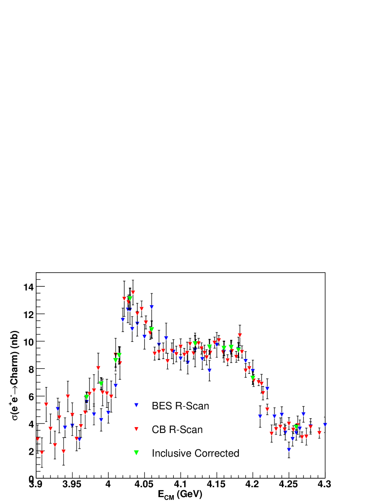
Figure 76: The radiatively corrected inclusive cross sections using the KF interpolation method on the CB data. The error bars include the systematics as discussed in the text.

Table 42: The total charm cross section as obtained by the inclusive method after being radiatively corrected. The errors are statistical and systematic respectively.

Ecm MeV	$\sigma(e^{+}e^{-}\rightarrow{D\bar{D}X})$ nb
3970	$5.92\pm 0.22\pm 0.28$
3990	$6.89\pm 0.25\pm 0.33$
4010	$8.60\pm 0.22\pm 0.41$
4015	$8.97\pm 0.42\pm 0.43$
4030	$13.10\pm 0.35\pm 0.63$
4060	$10.85\pm 0.28\pm 0.55$
4120	$9.82\pm 0.30\pm 0.49$
4140	$9.58\pm 0.22\pm 0.48$
4160	$9.48\pm 0.15\pm 0.48$
4170	$9.56\pm 0.07\pm 0.48$
4180	$9.36\pm 0.21\pm 0.47$
4200	$7.30\pm 0.25\pm 0.38$
4260	$3.73\pm 0.08\pm 0.20$

Figure 77: R measurement obtained from these inclusive charm cross sections, radiatively corrected, using the KF interpolation method on the CB data. The error bars include the systematics as discussed in the text.

Table 43: $R$, after being radiatively corrected, as determined by the inclusive method. The errors are statistical and systematic respectively. In this method we use $R_{uds}=2.285\pm 0.03$ as determined by a $\frac{1}{s}$ fit to previous $R$ measurements between 3.2 and 3.72 GeV.

Ecm MeV	$\frac{\sigma(e^{+}e^{-}\rightarrow{hadrons})}{\sigma(e^{+}e^{-}\rightarrow{\mu^{+}\mu^{-}})}$
3970	$3.36\pm 0.04\pm 0.05$
3990	$3.55\pm 0.05\pm 0.06$
4010	$3.88\pm 0.04\pm 0.08$
4015	$3.95\pm 0.08\pm 0.08$
4030	$4.74\pm 0.07\pm 0.12$
4060	$4.34\pm 0.05\pm 0.10$
4120	$4.21\pm 0.06\pm 0.10$
4140	$4.18\pm 0.04\pm 0.10$
4160	$4.18\pm 0.03\pm 0.10$
4170	$4.20\pm 0.01\pm 0.10$
4180	$4.17\pm 0.04\pm 0.10$
4200	$3.77\pm 0.05\pm 0.08$
4260	$3.06\pm 0.02\pm 0.04$

Chapter Interpretations and Conclusions

15 Comparisons

15.1 Comparisons to Previous Measurements

A comparison of the measurements reported in this thesis of $\sigma\cdot{{\cal{B}}}(D^{0}\rightarrow{K\pi})$ and $\sigma\cdot{{\cal{B}}}(D^{+}\rightarrow{K\pi\pi})$ with previous measurements is shown in Fig. 78. The results from the CLEO-c scan agree quite nicely with previous experiments, and are much more precise.

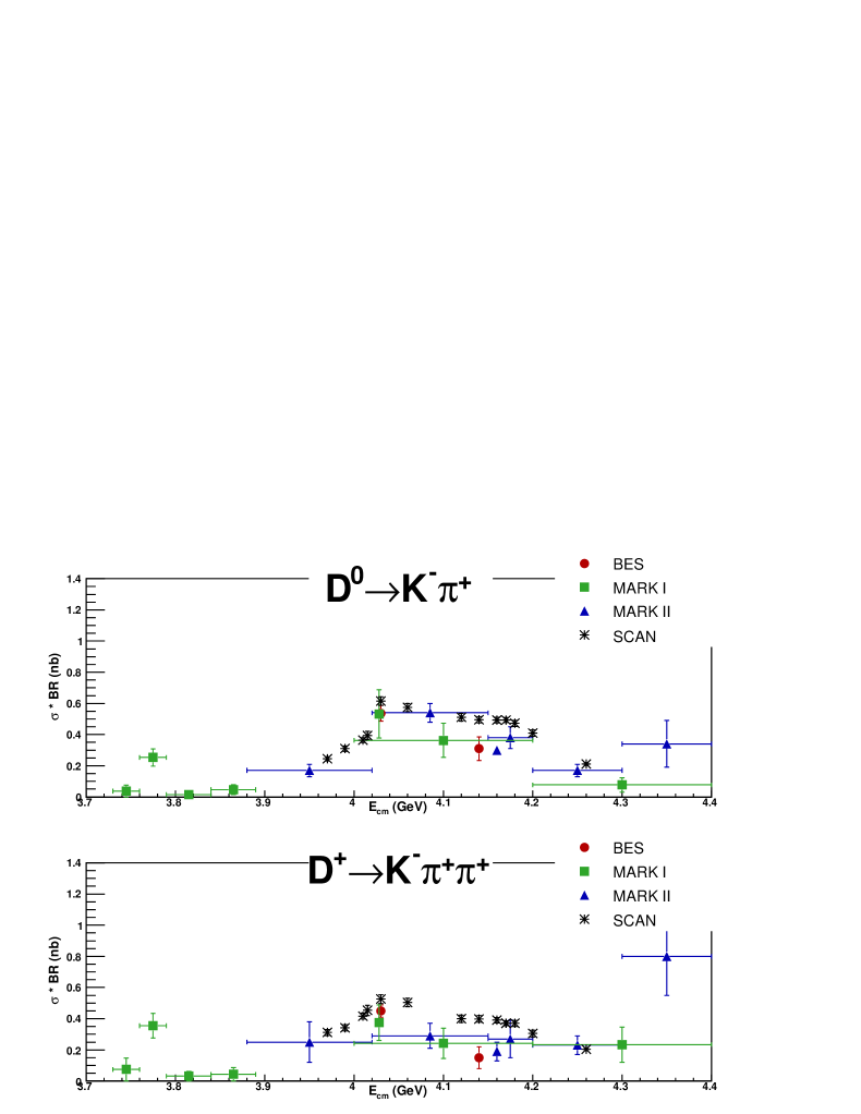
Figure 78: The production cross section times branching ratio for $D^{0}\rightarrow{K^{-}\pi^{+}}$ and $D^{0}\rightarrow{K^{-}\pi^{+}\pi^{+}}$ as a function of energy for this analysis, as compared to previous measurements. The results from the CLEO-c scan agree quite nicely with previous experiments.

In addition to the observed branching ratio times production cross section for $D^{0}$ and $D^{+}$, both Mark III and BES have made similar measurements involving the $D_{s}$. These results, BES [19] at center-of-mass energy of 4030 MeV and Mark III [20] at center-of-mass of 4140 MeV, are shown along with the results of this analysis in Table 44.

Table 44: Measurements of observed branching ratio times production cross sections. The first uncertainty in each case is statistical and the second (where given) is systematic.

Measurement	Energy (MeV)	Experiment
$\sigma_{D_{s}^{+}D_{s}^{-}}\cdot{{\cal{B}}}(D_{s}^{+}\rightarrow{\phi\pi^{+}})$
$11.2\pm 2.0\pm 2.5$ pb	4030	BES
$6.81\pm 2.48$ pb	4030	This Analysis
$\sigma_{D_{s}^{*+}D_{s}^{-}}\cdot{{\cal{B}}}(D_{s}^{+}\rightarrow{\phi\pi^{+}})$
$26\pm 6\pm 5$ pb	4140	MARK III
$36.1\pm 4.42$ pb	4140	This Analysis
$\sigma_{D_{s}^{*+}D_{s}^{-}}\cdot{{\cal{B}}}(D_{s}^{+}\rightarrow{\bar{K}^{0}K^{+}})$
$24\pm 6\pm 5$ pb	4140	MARK III
$23.1\pm 4.9$ pb	4140	This Analysis
$\sigma_{D_{s}^{*+}D_{s}^{-}}\cdot{{\cal{B}}}(D_{s}^{+}\rightarrow{\bar{K}^{*0}K^{+}})$
$22\pm 6\pm 6$ pb	4140	MARK III
$21.7\pm 4.0$ pb	4140	This Analysis

During the final preparation of this dissertation the Belle Collaboration [61] presented measurements of the cross sections for $D^{+}\bar{D}^{*-}$ and $D^{*+}\bar{D}^{*-}$ in the center-of-mass energy range from 3.7 to 5.0 GeV using ISR events produced in $e^{+}e^{-}$ annihilation at the $\Upsilon(4S)$. Their results are only for the charged $D$ pairs, so their results must be multiplied by a factor of 2 for comparison with the measurements presented in this thesis. Also, they present, up to higher-order radiative effects, Born-level cross sections. Based on a previous BaBar analysis [62], Belle estimated these higher-order corrections to be on the order of a percent. These small corrections are well within the systematic errors, which are $\sim$10%, and are therefore ignored. To do a comparison, I radiatively corrected the exclusive $D^{*}\bar{D}$ and $D^{*}\bar{D}^{*}$ from Tables 53 and 54 following the method described in Sect. Measurement of the Total Charm Cross Section by Electron-Positron Annihilation at Energies Between 3.97-4.26 GeV, where the shape of the cross section needed for the integral term was taken from Fig. 52. As can be seen by comparing Belle’s result (Fig. 79) to our result (Fig. 80) the agreement is quite good, keeping in mind the factor of two difference. It should be noted that their results cover a wider range of ${\rm{E_{CM}}}$, but are less precise than those present here.

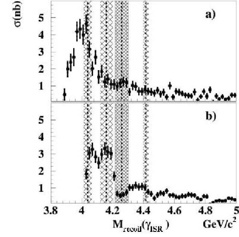
Figure 79: The exclusive cross sections for $e^{+}e^{-}\rightarrow{D^{+}}D^{*-}$ (top) and $e^{+}e^{-}\rightarrow{D^{*+}}D^{*-}$ from Belle [61]. The dashed lines correspond to the $\psi(4040)$, $\psi(4160)$, ${\rm{Y}}(4260)$, and $\psi(4415)$.

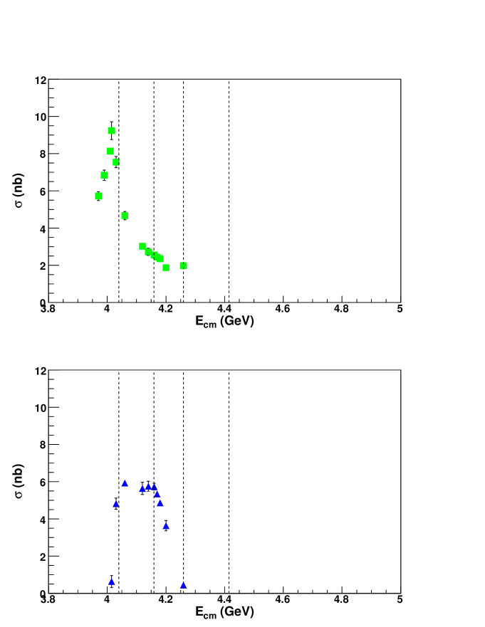
Figure 80: The exclusive cross sections for $e^{+}e^{-}\rightarrow{D}\bar{D}^{*}$ (top) and $e^{+}e^{-}\rightarrow{D^{*}}\bar{D}^{*}$, after applying radiative corrections, for the work presented in this dissertation. The dashed lines correspond to the $\psi(4040)$, $\psi(4160)$, ${\rm{Y}}(4260)$, and $\psi(4415)$. There is a factor of two difference between these results and those of Belle in Fig. 79.

In addition, the BaBar experiment [63] has presented data on the $D\bar{D}$ final state, also using the ISR technique in $e^{+}e^{-}$ annihilation at the $\Upsilon(4S)$. BaBar’s results are complicated by the fact that they combine several modes which have not been efficiency-corrected. Therefore, a direct comparison to their results is of limited value, because, the BaBar efficiency is acknowledged not to be flat as a function of the invariant mass. However, they do see a dip in the number of observed $D\bar{D}$ events in the neighborhood of 4015 MeV, which is in agreement with our observation.

Taking the partial widths calculated at $4160$ MeV by T. Barnes [28], which are reproduced in Table 5, and translating them into percentages, a comparison can be made to our results. This is shown in Table 45. The disagreement between the measurements and Barnes’s predictions are quite large, especially for $D\bar{D}$, $D^{*}\bar{D}$ and $D_{s}\bar{D}_{s}$.

Table 45: Percentages of event types present at center-of-mass energy of $4160$ MeV for this analysis as compared to the T. Branes predictions [28].

Center-of-Mass	$D\bar{D}$	$D^{*}\bar{D}$	$D^{*}\bar{D}^{*}$	$D_{s}^{+}{D_{s}^{-}}$	$D^{*+}_{s}{D^{-}_{s}}$
Energy (MeV)
$4160$ (This Analysis)	$3.9\pm 0.5$	$28.2\pm 1.8$	$54.1\pm 3.6$	$-$	$9.7\pm 0.6$
$4159$ (Barnes)	$21.6$	$0.5$	$47.3$	$10.8$	$18.9$

The analysis results for the cross sections two-body states (Figs. 81, 82) are in qualitative agreement with Eichten’s [27] prediction, Figs. 6 and 7. A more quantitative comparison with Eichten’s model awaits his updated calculations using the correct charmed-meson masses.

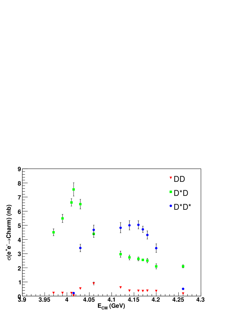
Figure 81: Results for the non-strange $D$-meson cross sections. The error bars include both statistical and systematic errors.

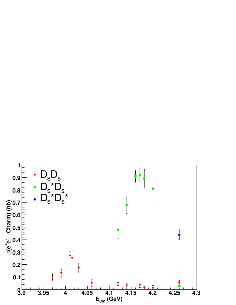
Figure 82: Results for the $D_{s}$-meson cross sections. The error bars include both statistical and systematic errors.

Recently, there has been work on the theoretical side in regards to the cross sections in the neighborhood of the $D^{*}\bar{D}^{*}$ threshold. Using very preliminary CLEO-c cross section results presented at the Flavor Physics and CP Violation Conference (FPCP) [64], Voloshin et al. [65, 66], using very general properties of amplitudes near a threshold, obtained resonance parameters assuming the cross sections between 3970 and 4060 MeV result from a single resonance. In their investigation they determined that the preliminary cross sections can not be described by a single resonance, but in fact hint at the presence of two, with one of the resonances being narrow. This can be found in their analysis when they struggled to describe the data by a single resonance which resulted in a $\chi^{2}/NDF=17.6/8$. They determined that if they ignored the data points for the cross section at 4010 and 4015 MeV for $D\bar{D}$ as well as $D^{*}\bar{D}^{*}$ at 4015 MeV a statistically significant result is obtained, $\chi^{2}/NDF=3.0/5.0$ Fig. 83. The reason for the poor fit when including all data points is almost solely due to the data point at 4015 MeV in $D\bar{D}$, where the value for the cross section is at a minimum. They suggest the existence of a new narrow resonance to describe this “dip” in the cross section. Following the same fit procedure as they described [66], results are updated to reflect the cross sections presented in this dissertation. These updated fits, shown in Fig. 84, still agree with their initial assessment, that is because of the large dip in the $D\bar{D}$ cross section a single resonance is insufficient in describing the cross sections near the $D^{*}\bar{D}^{*}$ threshold. The resonance parameters, with $D\bar{D}$ and $D^{*}\bar{D}^{*}$ at 4015 MeV left out the fit, are shown in Table 46.

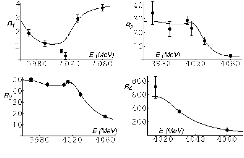
Figure 83: The fit results from Ref. [66] which used preliminary CLEO-c results. The data points that are excluded in the fit are shown with circles ($D\bar{D}$ at 4010 and 4015 MeV and $D^{*}\bar{D}^{*}$ at 4015 MeV). The fit are to dimensionless rate coefficients $R_{k}$ where $R_{k}\propto\sigma_{k}$ ($R_{1}$ (top left) corresponds to $D\bar{D}$, $R_{2}$ (top right) corresponds to $D_{s}\bar{D}_{s}$, $R_{3}$ (bottom left) corresponds to $D\bar{D}^{*}$, and $R_{4}$ (bottom right) corresponds to $D^{*}\bar{D}^{*}$).

Table 46: The resulting fit parameters from a single resonance fit to the cross sections, presented in this dissertation, around the $D^{*}\bar{D}^{*}$ threshold. The $D\bar{D}$ and $D^{*}\bar{D}^{*}$ data points were excluded in the fit resulting in $\chi^{2}/{\rm{NDF}}=3.8/6$. If all points were used the fit is quite poor, reflected in the resulting a $\chi^{2}/{\rm{NDF}}=36.3/8$, this is entirely because of $D\bar{D}$ at 4015 MeV.

Fit parameters	Result from Fit
$W_{0}$	$4013\pm 4$ MeV
$\Gamma_{0}$	$66\pm 8$ MeV
$w$	$10.4\pm 1.7$ MeV
$\Gamma_{D^{*}\bar{D}^{*}}$	$15.4\pm 1.3$ MeV
$\Gamma_{ee}$	$1.9\pm 0.7$ keV

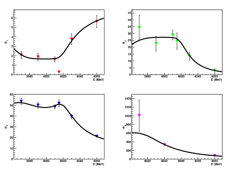
Figure 84: Fit results, assuming a single resonance [66], using the cross sections presented in this dissertation. The fit are to dimensionless rate coefficients $R_{k}$ where $R_{k}\propto\sigma_{k}$ ($R_{1}$ (top left) corresponds to $D\bar{D}$, $R_{2}$ (top right) corresponds to $D_{s}\bar{D}_{s}$, $R_{3}$ (bottom left) corresponds to $D\bar{D}^{*}$, and $R_{4}$ (bottom right) corresponds to $D^{*}\bar{D}^{*}$).

16 Conclusion

The CLEO-c scan was extremely successful in accomplishing the goals it put forth and as a result has provided a wealth of interesting results.

The location in center-of-mass energy that maximizes the yield of $D_{s}$ was determined by this analysis to be at 4170 MeV. The maximum occurs not with $D_{s}\bar{D}_{s}$ events, but rather with $D_{s}^{*}\bar{D}_{s}$ events. It is with this information that CLEO-c has already been able to make significant progress, on the decay constant and hadronic branching fractions of the $D_{s}$ meson [44, 67], with the data collected during the scan and in subsequent running at 4170 MeV.

The total charm cross section between $3.97$ GeV and $4.26$ GeV has been measured and presented. These results have been determined using three different techniques, the exclusive $D$-meson, inclusive $D$-meson, and inclusive hadron method, and are shown in Table 47 and graphically in Fig. 85. The agreement between these three different methods is very good and provides a powerful cross check on the results. Radiative corrections were determined and applied to the inclusive $D$ meson total charm result. The corrected cross sections are consistent with previous experimental results [18, 60] and are more precise (see Fig. 76).

The composition of the total charm cross section, in terms of $D\bar{D}$, $D^{*}\bar{D}$, $D^{*}\bar{D}^{*}$, $D_{s}\bar{D}_{s}$, $D_{s}^{*}\bar{D}_{s}$, $D_{s}^{*}\bar{D}_{s}^{*}$, $D^{*}\bar{D}\pi$ and $D^{*}\bar{D}^{*}\pi$, at all energies that were investigated, has been determined and presented. Results are shown in Tables 53 and 54, in addition to graphically in Figs. 81, 82, and 86. There is qualitative agreement with the potential model put forth by Eichten et al. [27] for all modes excluding the multi-body production, which was not predicted. The existence of a peak in the $D^{*}\bar{D}$ and $D_{s}\bar{D}_{s}$ channels at the $D^{*}\bar{D}^{*}$ threshold, along with the observation that there is a minimum in the $D\bar{D}$, can be interpreted as a possible new narrow resonance [66]. Unfortunately, the available data sample is insufficient to investigate this latter idea further.

The $D^{*}\bar{D}^{*}$ cross section shows a plateau region above its threshold, whereas the $D^{*}\bar{D}$ peaks right at the threshold, in agreement with the recently presented results by the Belle Collaboration [61].

Also, events containing $D$ mesons plus an additional pion, referred to as multi-body, have been shown to exists in the energy region investigated. Figs. 41, 42, and 43, show the cross sections that have been determined.

Using the data sample collected at 4260 MeV we searched for insight into the nature of the $Y(4260)$ state. By applying the techniques developed with the larger data sample collected at 4170 MeV we find that, besides the presence of the $D^{*}D^{*}\pi$ final state and larger overall production of multi-body, there is essentially nothing to distinguish the charm production at this energy from that at our lower-energy points. Although studies are still ongoing, we have preliminarily concluded that our data sample is insufficient to determine the contribution of states including excited charmed meson states (e.g. $D_{1}\bar{D}$) that are expected under some $Y(4260)$ interpretations [68].

As for the future, it is unlikely that time will be available to allow further investigation of the Y(4260) and region around the $D^{*}\bar{D}^{*}$ to be done at CLEO-c. However, the next stage in the BES experiment, BES-III [69], is planning to investigate in-depth the region around $D^{*}\bar{D}^{*}$ and should potentially be able to add insight to this region of interest. In addition to BES-III, both Belle and BaBar have shown that they too can investigate this region and we are impatiently awaiting their updated results.

Table 47: Comparison of the total charm cross section using the 3 different methods. First error is statistical and the second systematic.

Energy	Exclusive	Inclusive	Hadron
(MeV)	$D$-meson (nb)	$D$-meson (nb)	Counting (nb)
3970	$4.83\pm 0.19\pm 0.15$	$4.91\pm 0.18\pm 0.16$	$4.91\pm 0.13\pm 0.30$
3990	$5.85\pm 0.23\pm 0.19$	$5.93\pm 0.21\pm 0.19$	$5.87\pm 0.14\pm 0.34$
4010	$7.10\pm 0.14\pm 0.23$	$7.05\pm 0.17\pm 0.23$	$7.21\pm 0.12\pm 0.40$
4015	$7.94\pm 0.41\pm 0.26$	$7.62\pm 0.34\pm 0.25$	$7.88\pm 0.18\pm 0.43$
4030	$10.60\pm 0.34\pm 0.27$	$10.87\pm 0.28\pm 0.37$	$11.30\pm 0.15\pm 0.59$
4060	$10.16\pm 0.36\pm 0.27$	$9.98\pm 0.26\pm 0.34$	$9.98\pm 0.14\pm 0.53$
4120	$8.95\pm 0.37\pm 0.25$	$9.13\pm 0.28\pm 0.31$	$9.43\pm 0.15\pm 0.49$
4140	$9.22\pm 0.29\pm 0.26$	$9.11\pm 0.22\pm 0.30$	$9.58\pm 0.24\pm 0.50$
4160	$9.33\pm 0.20\pm 0.26$	$9.10\pm 0.15\pm 0.30$	$9.62\pm 0.17\pm 0.50$
4170	$9.03\pm 0.04\pm 0.25$	$9.09\pm 0.07\pm 0.30$	$9.45\pm 0.09\pm 0.49$
4180	$8.67\pm 0.27\pm 0.24$	$8.70\pm 0.20\pm 0.29$	$9.07\pm 0.12\pm 0.47$
4200	$7.42\pm 0.35\pm 0.20$	$7.45\pm 0.26\pm 0.25$	$8.37\pm 0.14\pm 0.43$
4260	$4.27\pm 0.16\pm 0.14$	$4.20\pm 0.10\pm 0.14$	$4.34\pm 0.16\pm 0.23$

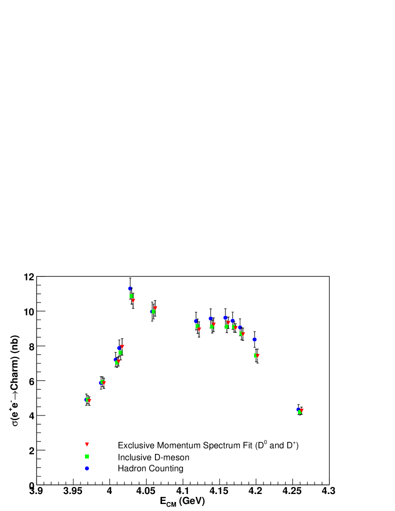
Figure 85: Comparison of the total charm cross section using the 3 different methods. This is a graphical representation of Table 47.

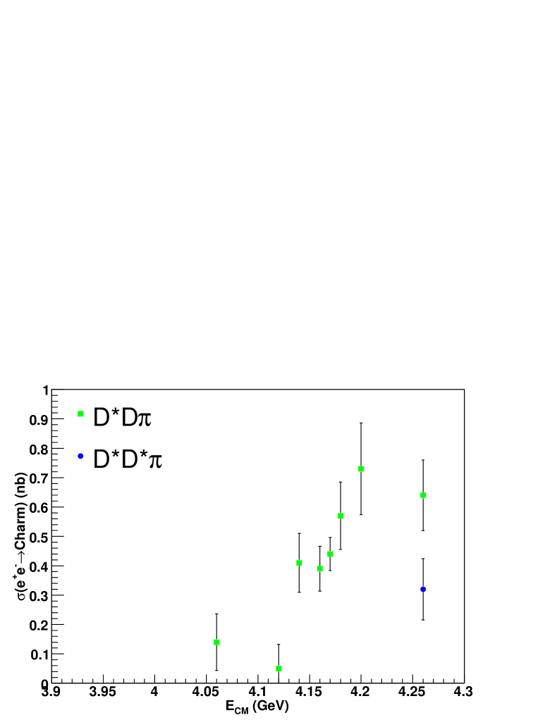
Figure 86: Results for the multi-body cross sections. The error bars include both statistical and systematic errors.

Table 48: Efficiencies (units of $10^{-2}$) at each scan-energy point for selection of $D_{s}^{+}$ through various decay modes in the three exclusive event types.

Mode	Ecm MeV	$D_{s}\bar{D}_{s}$	$D_{s}^{*}\bar{D}_{s}$	$D_{s}^{*}\bar{D}_{s}^{*}$
$K_{s}K^{+}$	$3970$	$56.2\pm 1.7$	$-\pm-$	$-\pm-$
	$3990$	$55.2\pm 1.7$	$-\pm-$	$-\pm-$
	$4010$	$57.0\pm 1.7$	$-\pm-$	$-\pm-$
	$4015$	$57.8\pm 1.4$	$-\pm-$	$-\pm-$
	$4030$	$58.3\pm 1.5$	$-\pm-$	$-\pm-$
	$4060$	$56.7\pm 1.5$	$-\pm-$	$-\pm-$
	$4120$	$57.6\pm 1.9$	$55.8\pm 1.3$	$-\pm-$
	$4140$	$50.6\pm 1.4$	$58.2\pm 0.9$	$-\pm-$
	$4160$	$54.3\pm 1.9$	$55.9\pm 1.3$	$-\pm-$
	$4180$	$52.1\pm 1.9$	$55.3\pm 1.3$	$-\pm-$
	$4200$	$52.9\pm 1.9$	$53.9\pm 1.4$	$-\pm-$
	$4260$	$62.0\pm 4.4$	$58.1\pm 3.1$	$56.4\pm 1.5$
$\eta\pi^{+}$	$3970$	$39.2\pm 2.3$	$-\pm-$	$-\pm-$
	$3990$	$39.3\pm 2.3$	$-\pm-$	$-\pm-$
	$4010$	$37.9\pm 2.2$	$-\pm-$	$-\pm-$
	$4015$	$42.0\pm 1.9$	$-\pm-$	$-\pm-$
	$4030$	$53.7\pm 2.1$	$-\pm-$	$-\pm-$
	$4060$	$39.7\pm 2.0$	$-\pm-$	$-\pm-$
	$4120$	$33.1\pm 2.4$	$38.3\pm 1.8$	$-\pm-$
	$4140$	$37.1\pm 1.8$	$40.7\pm 1.3$	$-\pm-$
	$4160$	$26.6\pm 2.3$	$38.3\pm 1.8$	$-\pm-$
	$4180$	$37.9\pm 2.5$	$38.8\pm 1.8$	$-\pm-$
	$4200$	$41.1\pm 2.6$	$34.9\pm 1.8$	$-\pm-$
	$4260$	$42.6\pm 6.0$	$39.2\pm 4.2$	$40.0\pm 2.0$
$\phi\pi^{+}$	$3970$	$42.7\pm 1.4$	$-\pm-$	$-\pm-$
	$3990$	$42.1\pm 1.4$	$-\pm-$	$-\pm-$
	$4010$	$42.9\pm 1.4$	$-\pm-$	$-\pm-$
	$4015$	$41.0\pm 1.1$	$-\pm-$	$-\pm-$
	$4030$	$43.8\pm 1.3$	$-\pm-$	$-\pm-$
	$4060$	$43.1\pm 1.3$	$-\pm-$	$-\pm-$
	$4120$	$39.6\pm 1.6$	$40.5\pm 1.1$	$-\pm-$
	$4140$	$39.8\pm 1.1$	$41.8\pm 0.8$	$-\pm-$
	$4160$	$41.6\pm 1.6$	$41.3\pm 1.1$	$-\pm-$
	$4180$	$36.7\pm 1.5$	$42.8\pm 1.1$	$-\pm-$
	$4200$	$42.7\pm 1.6$	$42.2\pm 1.1$	$-\pm-$
	$4260$	$43.8\pm 3.7$	$43.4\pm 2.6$	$41.8\pm 1.2$

Mode	Ecm MeV	$D_{s}\bar{D}_{s}$	$D_{s}^{*}\bar{D}_{s}$	$D_{s}^{*}\bar{D}_{s}^{*}$
$K^{*}K^{+}$	$3970$	$39.1\pm 1.2$	$-\pm-$	$-\pm-$
	$3990$	$40.0\pm 1.2$	$-\pm-$	$-\pm-$
	$4010$	$42.5\pm 1.2$	$-\pm-$	$-\pm-$
	$4015$	$41.3\pm 1.0$	$-\pm-$	$-\pm-$
	$4030$	$42.0\pm 1.1$	$-\pm-$	$-\pm-$
	$4060$	$41.5\pm 1.1$	$-\pm-$	$-\pm-$
	$4120$	$40.1\pm 1.4$	$40.8\pm 1.0$	$-\pm-$
	$4140$	$39.2\pm 1.0$	$42.0\pm 0.7$	$-\pm-$
	$4160$	$42.7\pm 1.4$	$42.0\pm 1.0$	$-\pm-$
	$4180$	$43.3\pm 1.4$	$42.6\pm 1.0$	$-\pm-$
	$4200$	$37.7\pm 1.4$	$41.6\pm 1.0$	$-\pm-$
	$4260$	$41.2\pm 3.2$	$35.0\pm 2.2$	$41.4\pm 1.1$
$\eta\rho^{+}$	$3970$	$19.2\pm 0.7$	$-\pm-$	$-\pm-$
	$3990$	$17.1\pm 0.7$	$-\pm-$	$-\pm-$
	$4010$	$16.8\pm 0.7$	$-\pm-$	$-\pm-$
	$4015$	$16.9\pm 0.6$	$-\pm-$	$-\pm-$
	$4030$	$24.0\pm 0.7$	$-\pm-$	$-\pm-$
	$4060$	$16.5\pm 0.6$	$-\pm-$	$-\pm-$
	$4120$	$16.7\pm 0.8$	$16.9\pm 0.5$	$-\pm-$
	$4140$	$17.1\pm 0.6$	$16.0\pm 0.4$	$-\pm-$
	$4160$	$14.9\pm 0.7$	$16.1\pm 0.5$	$-\pm-$
	$4180$	$16.3\pm 0.8$	$16.2\pm 0.5$	$-\pm-$
	$4200$	$16.9\pm 0.8$	$17.1\pm 0.6$	$-\pm-$
	$4260$	$15.4\pm 1.8$	$18.7\pm 1.3$	$17.4\pm 0.6$
$\eta^{{}^{\prime}}\pi^{+}$	$3970$	$31.9\pm 2.1$	$-\pm-$	$-\pm-$
	$3990$	$33.2\pm 2.2$	$-\pm-$	$-\pm-$
	$4010$	$30.9\pm 2.1$	$-\pm-$	$-\pm-$
	$4015$	$34.8\pm 1.8$	$-\pm-$	$-\pm-$
	$4030$	$32.4\pm 1.9$	$-\pm-$	$-\pm-$
	$4060$	$26.7\pm 1.8$	$-\pm-$	$-\pm-$
	$4120$	$21.2\pm 2.1$	$28.8\pm 1.7$	$-\pm-$
	$4140$	$27.6\pm 1.6$	$25.8\pm 1.1$	$-\pm-$
	$4160$	$29.2\pm 2.4$	$29.9\pm 1.7$	$-\pm-$
	$4180$	$29.9\pm 2.4$	$32.8\pm 1.7$	$-\pm-$
	$4200$	$29.5\pm 2.4$	$29.8\pm 1.7$	$-\pm-$
	$4260$	$16.1\pm 4.5$	$35.0\pm 4.1$	$28.2\pm 1.8$

Mode	Ecm MeV	$D_{s}\bar{D}_{s}$	$D_{s}^{*}\bar{D}_{s}$	$D_{s}^{*}\bar{D}_{s}^{*}$
$\eta^{{}^{\prime}}\rho^{+}$	$3970$	$16.0\pm 1.1$	$-\pm-$	$-\pm-$
	$3990$	$12.9\pm 1.0$	$-\pm-$	$-\pm-$
	$4010$	$13.4\pm 1.0$	$-\pm-$	$-\pm-$
	$4015$	$13.7\pm 0.8$	$-\pm-$	$-\pm-$
	$4030$	$13.0\pm 0.9$	$-\pm-$	$-\pm-$
	$4060$	$11.6\pm 0.8$	$-\pm-$	$-\pm-$
	$4120$	$11.7\pm 1.0$	$14.2\pm 0.8$	$-\pm-$
	$4140$	$12.0\pm 0.7$	$12.5\pm 0.5$	$-\pm-$
	$4160$	$11.1\pm 1.0$	$11.8\pm 0.7$	$-\pm-$
	$4180$	$15.0\pm 1.2$	$12.1\pm 0.7$	$-\pm-$
	$4200$	$14.0\pm 1.1$	$13.3\pm 0.8$	$-\pm-$
	$4260$	$14.2\pm 2.0$	$14.9\pm 1.9$	$15.0\pm 0.9$
$\phi\rho^{+}$	$3970$	$13.6\pm 0.7$	$-\pm-$	$-\pm-$
	$3990$	$13.4\pm 0.7$	$-\pm-$	$-\pm-$
	$4010$	$13.4\pm 0.7$	$-\pm-$	$-\pm-$
	$4015$	$12.9\pm 0.6$	$-\pm-$	$-\pm-$
	$4030$	$15.5\pm 0.7$	$-\pm-$	$-\pm-$
	$4060$	$12.6\pm 0.6$	$-\pm-$	$-\pm-$
	$4120$	$13.7\pm 0.8$	$12.5\pm 0.6$	$-\pm-$
	$4140$	$14.2\pm 0.6$	$11.8\pm 0.4$	$-\pm-$
	$4160$	$14.9\pm 0.8$	$12.3\pm 0.5$	$-\pm-$
	$4180$	$15.6\pm 0.9$	$13.4\pm 0.6$	$-\pm-$
	$4200$	$15.8\pm 0.9$	$13.6\pm 0.6$	$-\pm-$
	$4260$	$15.2\pm 2.0$	$15.5\pm 1.4$	$11.0\pm 0.6$

Table 49: Numbers of events at E${}_{cm}=3671$ MeV for various event types which are used for continuum subtraction in the Hadron Counting Method to determine the total charm cross section.

Off-Res Data	$244663\pm 495$
B.W. Tail of $\psi(2S)$	$7201\pm 493$
Radiative Return to $J/\psi$	$10240\pm 157$
$\tau^{+}\tau^{-}$	$9227\pm 55$
$e^{+}e^{-}$	$3058\pm 649$
$\mu^{+}\mu^{-}$	$184\pm 21$
Efficiency Corrected Num. of $q\bar{q}$	$378420\pm 1934$

Table 50: Numbers of events at the scan energies for various event types which are used in the Hadron Counting Method to determine the total charm cross section.

E${}_{cm}=3970$ MeV
Number of Raw Hadronic Events	$60811\pm 247$
Scaled $q\bar{q}$	$38041\pm 233$
Radiative Return to $\psi(2S)$	$2352\pm 11$
Radiative Return to $J/\psi$	$1059\pm 8$
Radiative Return to $\psi(3770)$	$332\pm 1$
$\tau^{+}\tau^{-}$	$2915\pm 98$
$e^{+}e^{-}$	$340\pm 133$
$\mu^{+}\mu^{-}$	$32\pm 5$
Number of Beam Gas Events	$439\pm 102$
Efficiency Corrected Num.	$18926\pm 485$
E${}_{cm}=3990$ MeV
Number of Raw Hadronic Events	$54818\pm 234$
Scaled $q\bar{q}$	$32649\pm 201$
Radiative Return to $\psi(2S)$	$1869\pm 9$
Radiative Return to $J/\psi$	$889\pm 6$
Radiative Return to $\psi(3770)$	$264\pm 1$
$\tau^{+}\tau^{-}$	$2365\pm 84$
$e^{+}e^{-}$	$471\pm 140$
$\mu^{+}\mu^{-}$	$28\pm 5$
Number of Beam Gas Events	$341\pm 122$
Efficiency Corrected Num.	$19696\pm 458$
E${}_{cm}=4010$ MeV
Number of Raw Hadronic Events	$97629\pm 312$
Scaled $q\bar{q}$	$54635\pm 327$
Radiative Return to $\psi(2S)$	$2929\pm 13$
Radiative Return to $J/\psi$	$1429\pm 10$
Radiative Return to $\psi(3770)$	$408\pm 2$
$\tau^{+}\tau^{-}$	$4128\pm 144$
$e^{+}e^{-}$	$635\pm 212$
$\mu^{+}\mu^{-}$	$46\pm 8$
Number of Beam Gas Events	$565\pm 173$
Efficiency Corrected Num.	$40539\pm 679$

E${}_{cm}=4015$ MeV
Number of Raw Hadronic Events	$26436\pm 163$
Scaled $q\bar{q}$	$14240\pm 96$
Radiative Return to $\psi(2S)$	$753\pm 4$
Radiative Return to $J/\psi$	$371\pm 3$
Radiative Return to $\psi(3770)$	$106\pm 1$
$\tau^{+}\tau^{-}$	$1137\pm 39$
$e^{+}e^{-}$	$165\pm 55$
$\mu^{+}\mu^{-}$	$12\pm 2$
Number of Beam Gas Events	$152\pm 87$
Efficiency Corrected Num.	$11581\pm 267$
E${}_{cm}=4030$ MeV
Number of Raw Hadronic Events	$62354\pm 250$
Scaled $q\bar{q}$	$29017\pm 180$
Radiative Return to $\psi(2S)$	$1460\pm 7$
Radiative Return to $J/\psi$	$733\pm 5$
Radiative Return to $\psi(3770)$	$197\pm 1$
$\tau^{+}\tau^{-}$	$2252\pm 78$
$e^{+}e^{-}$	$593\pm 145$
$\mu^{+}\mu^{-}$	$25\pm 4$
Number of Beam Gas Events	$285\pm 127$
Efficiency Corrected Num.	$33955\pm 457$
E${}_{cm}=4060$ MeV
Number of Raw Hadronic Events	$64117\pm 253$
Scaled $q\bar{q}$	$31305\pm 193$
Radiative Return to $\psi(2S)$	$1467\pm 7$
Radiative Return to $J/\psi$	$797\pm 6$
Radiative Return to $\psi(3770)$	$194\pm 1$
$\tau^{+}\tau^{-}$	$2582\pm 87$
$e^{+}e^{-}$	$277\pm 108$
$\mu^{+}\mu^{-}$	$26\pm 4$
Number of Beam Gas Events	$345\pm 139$
Efficiency Corrected Num.	$32803\pm 455$

E${}_{cm}=4120$ MeV
Number of Raw Hadronic Events	$51863\pm 228$
Scaled $q\bar{q}$	$25694\pm 161$
Radiative Return to $\psi(2S)$	$1027\pm 5$
Radiative Return to $J/\psi$	$552\pm 4$
Radiative Return to $\psi(3770)$	$126\pm 1$
$\tau^{+}\tau^{-}$	$2210\pm 74$
$e^{+}e^{-}$	$462\pm 118$
$\mu^{+}\mu^{-}$	$22\pm 4$
Number of Beam Gas Events	$280\pm 131$
Efficiency Corrected Num.	$26016\pm 411$
E${}_{cm}=4140$ MeV
Number of Raw Hadronic Events	$91780\pm 303$
Scaled $q\bar{q}$	$45202\pm 220$
Radiative Return to $\psi(2S)$	$1705\pm 7$
Radiative Return to $J/\psi$	$954\pm 6$
Radiative Return to $\psi(3770)$	$221\pm 1$
$\tau^{+}\tau^{-}$	$3585\pm 100$
$e^{+}e^{-}$	$739\pm 162$
$\mu^{+}\mu^{-}$	$38\pm 5$
Number of Beam Gas Events	$518\pm 163$
Efficiency Corrected Num.	$46910\pm 548$
E${}_{cm}=4160$ MeV
Number of Raw Hadronic Events	$190764\pm 437$
Scaled $q\bar{q}$	$93833\pm 398$
Radiative Return to $\psi(2S)$	$3467\pm 11$
Radiative Return to $J/\psi$	$1876\pm 11$
Radiative Return to $\psi(3770)$	$400\pm 2$
$\tau^{+}\tau^{-}$	$7761\pm 192$
$e^{+}e^{-}$	$1417\pm 301$
$\mu^{+}\mu^{-}$	$78\pm 9$
Number of Beam Gas Events	$1019\pm 212$
Efficiency Corrected Num.	$97750\pm 879$

E${}_{cm}=4170$ MeV
Number of Raw Hadronic Events	$3301243\pm 1817$
Scaled $q\bar{q}$	$1641982\pm 9325$
Radiative Return to $\psi(2S)$	$59506\pm 239$
Radiative Return to $J/\psi$	$33037\pm 252$
Radiative Return to $\psi(3770)$	$7001\pm 28$
$\tau^{+}\tau^{-}$	$138524\pm 4746$
$e^{+}e^{-}$	$24731\pm 7419$
$\mu^{+}\mu^{-}$	$1361\pm 227$
Number of Beam Gas Events	$5256.47\pm 205.89$
Efficiency Corrected Num.	$1683110\pm 15884$
E${}_{cm}=4180$ MeV
Number of Raw Hadronic Events	$103834\pm 322$
Scaled $q\bar{q}$	$52037\pm 310$
Radiative Return to $\psi(2S)$	$1806\pm 8$
Radiative Return to $J/\psi$	$1009\pm 8$
Radiative Return to $\psi(3770)$	$221\pm 1$
$\tau^{+}\tau^{-}$	$4744\pm 156$
$e^{+}e^{-}$	$840\pm 234$
$\mu^{+}\mu^{-}$	$43\pm 7$
Number of Beam Gas Events	$613\pm 131$
Efficiency Corrected Num.	$51410\pm 662$
E${}_{cm}=4200$ MeV
Number of Raw Hadronic Events	$49296\pm 222$
Scaled $q\bar{q}$	$25592\pm 161$
Radiative Return to $\psi(2S)$	$852\pm 4$
Radiative Return to $J/\psi$	$470\pm 4$
Radiative Return to $\psi(3770)$	$109\pm 1$
$\tau^{+}\tau^{-}$	$2159\pm 75$
$e^{+}e^{-}$	$291\pm 97$
$\mu^{+}\mu^{-}$	$21\pm 4$
Number of Beam Gas Events	$329\pm 131$
Efficiency Corrected Num.	$23509\pm 397$

E${}_{cm}=4260$ MeV
Number of Raw Hadronic Events	$183192\pm 427$
Scaled $q\bar{q}$	$117111\pm 520$
Radiative Return to $\psi(2S)$	$3477\pm 11$
Radiative Return to $J/\psi$	$1811\pm 12$
Radiative Return to $\psi(3770)$	$424\pm 2$
$\tau^{+}\tau^{-}$	$10239\pm 267$
$e^{+}e^{-}$	$2178\pm 426$
$\mu^{+}\mu^{-}$	$97\pm 12$
Number of Beam Gas Events	$906\pm 262$
Efficiency Corrected Num.	$56787\pm 1066$

Figure 106: Sideband-subtracted momentum spectrum for $D^{+}\rightarrow{K^{-}}\pi^{+}\pi^{+}$ at 4180 MeV. The data is the points with error bars and the histograms are MC.

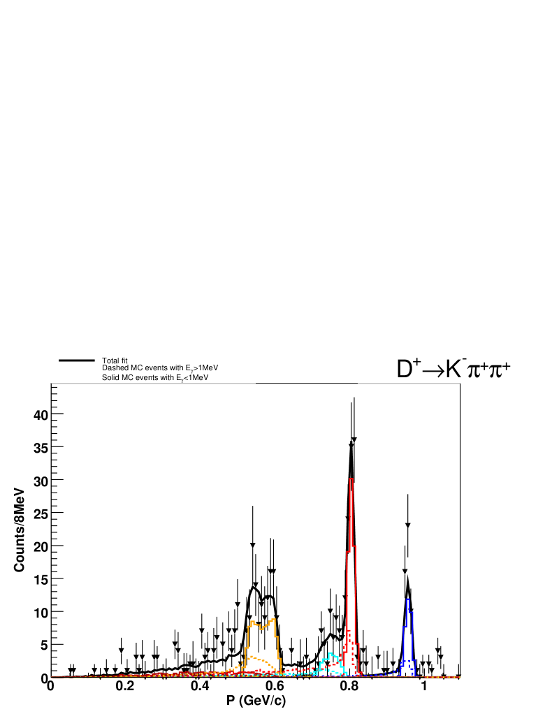
Figure 108: Sideband-subtracted momentum spectrum for $D^{+}\rightarrow{K^{-}}\pi^{+}\pi^{+}$ at 4200 MeV. The data is the points with error bars and the histograms are MC.

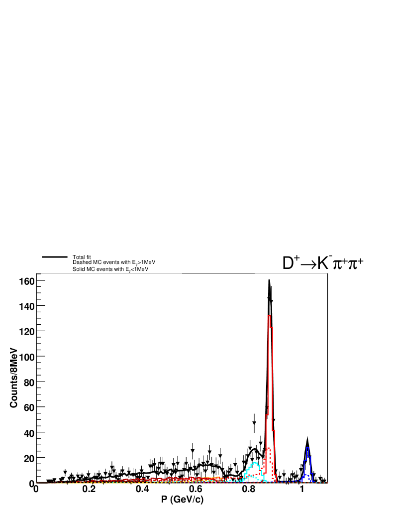
Figure 110: Sideband-subtracted momentum spectrum for $D^{+}\rightarrow{K^{-}}\pi^{+}\pi^{+}$ at 4260 MeV. The data is the points with error bars and the histograms are MC.

Figure 111: Sideband-subtracted momentum spectrum for $D_{s}^{+}\rightarrow\phi\pi^{+}$ at 3970 MeV. The data is the points with error bars and the histograms are MC.

Figure 113: Sideband-subtracted momentum spectrum for $D_{s}^{+}\rightarrow\phi\pi^{+}$ at 4010 MeV. The data is the points with error bars and the histograms are MC.

Table 51: Observed cross sections for various center of mass energies as determined by the cut and count method described in the text. All error are statistical and cross sections shown are the weighted sums or averages for the event types.

Cross Section	$3970$ MeV	$3990$ MeV	$4010$ MeV	$4015$ MeV	$4030$ MeV	$4060$ MeV
	${\cal{L}}$$=3.85$ pb-1	${\cal{L}}$$=3.36$ pb-1	${\cal{L}}$$=5.63$ pb-1	${\cal{L}}$$=1.47$ pb-1	${\cal{L}}$$=3.01$ pb-1	${\cal{L}}$$=3.29$ pb-1
$\sigma({D_{s}D_{s}})$ nb	$0.102\pm 0.026$	$0.133\pm 0.031$	$0.269\pm 0.030$	$0.250\pm 0.059$	$0.174\pm 0.036$	$0.051\pm 0.028$
$\sigma({D_{s}^{*}D_{s}})$ nb	$-\pm-$	$-\pm-$	$-\pm-$	$-\pm-$	$-\pm-$	$-\pm-$
$\sigma({D_{s}^{*}D_{s}^{*}})$ nb	$-\pm-$	$-\pm-$	$-\pm-$	$-\pm-$	$-\pm-$	$-\pm-$
$\sigma({D{D}})$ nb	$0.194\pm 0.027$	$0.146\pm 0.027$	$0.085\pm 0.020$	$0.037\pm 0.033$	$0.410\pm 0.037$	$0.615\pm 0.041$
$\sigma({D^{*}D})$ nb	$4.289\pm 0.117$	$5.105\pm 0.136$	$6.285\pm 0.116$	$6.999\pm 0.236$	$6.200\pm 0.163$	$3.687\pm 0.129$
$\sigma({D^{*}D^{*}})$ nb	$-\pm-$	$-\pm-$	$-\pm-$	$0.153\pm 0.035$	$3.745\pm 0.151$	$4.779\pm 0.189$
$\sigma(Charm)$ nb	$4.585\pm 0.123$	$5.384\pm 0.142$	$6.639\pm 0.121$	$7.439\pm 0.248$	$10.529\pm 0.228$	$9.132\pm 0.234$

Table 52: Observed cross sections for various center of mass energies as determined by the cut and count method described in the text. All error are statistical and cross sections shown are the weighted sums or averages for the event types.

Cross Section	$4120$ MeV	$4140$ MeV	$4160$ MeV	$4180$ MeV	$4200$ MeV	$4260$ MeV
	${\cal{L}}$$=2.76$ pb-1	${\cal{L}}$$=4.87$ pb-1	${\cal{L}}$$=10.16$ pb-1	${\cal{L}}$$=5.67$ pb-1	${\cal{L}}$$=2.81$ pb-1	${\cal{L}}$$=13.11$ pb-1
$\sigma({D_{s}D_{s}})$ nb	$0.026\pm 0.026$	$0.025\pm 0.020$	$-0.008\pm 0.012$	$0.007\pm 0.016$	$0.015\pm 0.022$	$0.034\pm 0.009$
$\sigma({D_{s}^{*}D_{s}})$ nb	$0.478\pm 0.064$	$0.684\pm 0.059$	$0.905\pm 0.044$	$0.889\pm 0.059$	$0.812\pm 0.082$	$0.047\pm 0.022$
$\sigma({D_{s}^{*}D_{s}^{*}})$ nb	$-\pm-$	$-\pm-$	$-\pm-$	$-\pm-$	$-\pm-$	$0.440\pm 0.027$
$\sigma({D{D}})$ nb	$0.466\pm 0.039$	$0.328\pm 0.026$	$0.267\pm 0.017$	$0.249\pm 0.022$	$0.295\pm 0.032$	$0.105\pm 0.011$
$\sigma({D^{*}D})$ nb	$2.481\pm 0.122$	$2.243\pm 0.090$	$2.100\pm 0.061$	$1.951\pm 0.079$	$1.615\pm 0.107$	$1.407\pm 0.047$
$\sigma({D^{*}D^{*}})$ nb	$5.073\pm 0.213$	$4.868\pm 0.165$	$5.153\pm 0.117$	$4.620\pm 0.147$	$3.730\pm 0.197$	$1.142\pm 0.059$
$\sigma(Charm)$ nb	$8.524\pm 0.258$	$8.148\pm 0.200$	$8.417\pm 0.141$	$7.716\pm 0.179$	$6.467\pm 0.242$	$3.175\pm 0.084$

Table 53: Observed cross sections for various center of mass energies as determined by fits to the $D^{0}$ and $D^{+}$ momentum spectra. The $D_{s}$ cross sections are determined using a weighted sum techneque discribed in Sect. 9. The first error is statistical and the second is systematic.

Cross Section	$3970$MeV	$3990$MeV	$4010$MeV
	${\cal{L}}$$=3.85$pb-1	${\cal{L}}$$=3.36$pb-1	${\cal{L}}$$=5.63$pb-1
$\sigma({D_{s}D_{s}})$ nb	$0.102\pm 0.026\pm 0.006$	$0.133\pm 0.031\pm 0.007$	$0.269\pm 0.030\pm 0.015$
$\sigma({D_{s}^{*}D_{s}})$ nb	$-\pm-\pm-$	$-\pm-\pm-$	$-\pm-\pm-$
$\sigma({D_{s}^{*}D_{s}^{*}})$ nb	$-\pm-\pm-$	$-\pm-\pm-$	$-\pm-\pm-$
$\sigma({D{D}})$ nb	$0.223\pm 0.039\pm 0.010$	$0.223\pm 0.047\pm 0.010$	$0.211\pm 0.033\pm 0.009$
$\sigma({D^{*}D})$ nb	$4.510\pm 0.187\pm 0.153$	$5.490\pm 0.221\pm 0.187$	$6.620\pm 0.133\pm 0.225$
$\sigma({D^{*}D^{*}})$ nb	$-\pm-\pm-$	$-\pm-\pm-$	$-\pm-\pm-$
$\sigma({D^{*}D\pi})$ nb	$-\pm-\pm-$	$-\pm-\pm-$	$-\pm-\pm-$
$\sigma({D^{*}D^{*}\pi})$ nb	$-\pm-\pm-$	$-\pm-\pm-$	$-\pm-\pm-$
$\sigma(Charm)$ nb	$4.835\pm 0.193\pm 0.154$	$5.846\pm 0.228\pm 0.187$	$7.100\pm 0.140\pm 0.226$
Cross Section	$4015$MeV	$4030$MeV	$4060$MeV
	${\cal{L}}$$=1.47$pb-1	${\cal{L}}$$=3.01$pb-1	${\cal{L}}$$=3.29$pb-1
$\sigma({D_{s}D_{s}})$ nb	$0.250\pm 0.059\pm 0.014$	$0.174\pm 0.036\pm 0.010$	$0.051\pm 0.028\pm 0.003$
$\sigma({D_{s}^{*}D_{s}})$ nb	$-\pm-\pm-$	$-\pm-\pm-$	$-\pm-\pm-$
$\sigma({D_{s}^{*}D_{s}^{*}})$ nb	$-\pm-\pm-$	$-\pm-\pm-$	$-\pm-\pm-$
$\sigma({D{D}})$ nb	$0.038\pm 0.020\pm 0.002$	$0.530\pm 0.078\pm 0.024$	$0.890\pm 0.091\pm 0.040$
$\sigma({D^{*}D})$ nb	$7.443\pm 0.394\pm 0.256$	$6.500\pm 0.257\pm 0.221$	$4.400\pm 0.205\pm 0.150$
$\sigma({D^{*}D^{*}})$ nb	$0.213\pm 0.076\pm 0.009$	$3.400\pm 0.211\pm 0.160$	$4.680\pm 0.258\pm 0.220$
$\sigma({D^{*}D\pi})$ nbw	$-\pm-\pm-$	$-\pm-\pm-$	$0.144\pm 0.094\pm 0.017$
$\sigma({D^{*}D^{*}\pi})$ nb	$-\pm-\pm-$	$-\pm-\pm-$	$-\pm-\pm-$
$\sigma(Charm)$ nb	$7.941\pm 0.406\pm 0.257$	$10.604\pm 0.344\pm 0.274$	$10.165\pm 0.356\pm 0.270$

Table 54: Observed cross sections for various center of mass energies as determined by fits to the $D^{0}$ and $D^{+}$ momentum spectra. The $D_{s}$ cross sections are determined using a weighted sum techneque discribed in Sect. 9. The first error is statistical and the second is systematic.

Cross Section	$4120$MeV	$4140$MeV	$4160$MeV	$4170$MeV
	${\cal{L}}$$=2.76$pb-1	${\cal{L}}$$=4.87$pb-1	${\cal{L}}$$=10.16$pb-1	${\cal{L}}$$=178.9$pb-1
$\sigma({D_{s}D_{s}})$ nb	$0.026\pm 0.026\pm 0.001$	$0.025\pm 0.020\pm 0.001$	$-0.008\pm 0.012\pm 0.000$	$0.034\pm 0.003\pm 0.002$
$\sigma({D_{s}^{*}D_{s}})$ nb	$0.478\pm 0.064\pm 0.025$	$0.684\pm 0.059\pm 0.036$	$0.905\pm 0.011\pm 0.048$	$0.916\pm 0.011\pm 0.049$
$\sigma({D_{s}^{*}D_{s}^{*}})$ nb	$-\pm-\pm-$	$-\pm-\pm-$	$-\pm-\pm-$	$-\pm-\pm-$
$\sigma({D{D}})$ nb	$0.613\pm 0.086\pm 0.028$	$0.377\pm 0.049\pm 0.017$	$0.367\pm 0.035\pm 0.017$	$0.360\pm 0.010\pm 0.016$
$\sigma({D^{*}D})$ nb	$2.960\pm 0.192\pm 0.101$	$2.726\pm 0.140\pm 0.093$	$2.628\pm 0.098\pm 0.089$	$2.560\pm 0.030\pm 0.087$
$\sigma({D^{*}D^{*}})$ nb	$4.830\pm 0.278\pm 0.227$	$4.999\pm 0.228\pm 0.235$	$5.045\pm 0.159\pm 0.237$	$4.720\pm 0.030\pm 0.222$
$\sigma({D^{*}D\pi})$ nb	$0.045\pm 0.083\pm 0.005$	$0.412\pm 0.087\pm 0.049$	$0.389\pm 0.060\pm 0.047$	$0.440\pm 0.020\pm 0.053$
$\sigma({D^{*}D^{*}\pi})$ nb	$-\pm-\pm-$	$-\pm-\pm-$	$-\pm-\pm-$	$-\pm-\pm-$
$\sigma(Charm)$ nb	$8.952\pm 0.365\pm 0.251$	$9.223\pm 0.292\pm 0.260$	$9.326\pm 0.200\pm 0.263$	$9.03\pm 0.044\pm 0.250$
Cross Section	$4180$MeV	$4200$MeV	$4260$MeV
	${\cal{L}}$$=5.67$pb-1	${\cal{L}}$$=2.81$pb-1	${\cal{L}}$$=13.11$pb-1
$\sigma({D_{s}D_{s}})$ nb	$0.007\pm 0.016\pm 0.000$	$0.015\pm 0.022\pm 0.001$	$0.047\pm 0.022\pm 0.003$
$\sigma({D_{s}^{*}D_{s}})$ nb	$0.889\pm 0.059\pm 0.047$	$0.812\pm 0.082\pm 0.043$	$0.034\pm 0.009\pm 0.002$
$\sigma({D_{s}^{*}D_{s}^{*}})$ nb	$-\pm-\pm-$	$-\pm-\pm-$	$0.440\pm 0.027\pm 0.030$
$\sigma({D{D}})$ nb	$0.376\pm 0.047\pm 0.017$	$0.361\pm 0.066\pm 0.016$	$0.180\pm 0.022\pm 0.008$
$\sigma({D^{*}D})$ nb	$2.507\pm 0.127\pm 0.085$	$2.100\pm 0.169\pm 0.071$	$2.102\pm 0.080\pm 0.071$
$\sigma({D^{*}D^{*}})$ nb	$4.318\pm 0.201\pm 0.203$	$3.394\pm 0.256\pm 0.160$	$0.506\pm 0.069\pm 0.024$
$\sigma({D^{*}D\pi})$ nb	$0.575\pm 0.092\pm 0.069$	$0.735\pm 0.129\pm 0.088$	$0.638\pm 0.093\pm 0.077$
$\sigma({D^{*}D^{*}\pi})$ nb	$-\pm-\pm-$	$-\pm-\pm-$	$0.322\pm 0.067\pm 0.080$
$\sigma(Charm)$ nb	$8.672\pm 0.266\pm 0.236$	$7.417\pm 0.350\pm 0.201$	$4.269\pm 0.162\pm 0.138$

Chapter Helicity Formalism and Angular Distributions

In the spirit of obtaining the best possible MC sample a considerable amount of time was spent on determining the final-state angular distributions for each of the event types and the subsequent decays of the starred states. There are three different and distinct types of events that need to be considered:

• $1^{-}\rightarrow{0^{-}0^{-}}$, as in $e^{+}e^{-}\rightarrow\gamma^{*}\rightarrow{D\bar{D}}$

• $1^{-}\rightarrow{0^{-}1^{-}}$, as in $e^{+}e^{-}\rightarrow\gamma^{*}\rightarrow{D\bar{D}^{*}}$

• $1^{-}\rightarrow{1^{-}1^{-}}$, as in $e^{+}e^{-}\rightarrow\gamma^{*}\rightarrow{D^{*}\bar{D}^{*}}$

In addition to the above, there are also the subsequent decays:

• $1^{-}\rightarrow{1^{-}0^{-}}$, as in $D^{*}\rightarrow{\gamma{D}}$

• $1^{-}\rightarrow{0^{-}0^{-}}$, as in $D^{*}\rightarrow{\pi{D}}$

Each of the above cases, except $1^{-}\rightarrow{0^{-}0^{-}}$, since it is already understood from $\psi(3770)$ running (for completeness its distribution is $\sin^{2}\theta$), is described individually below using the helicity formalism as discussed by J.D. Richman in Ref. [70]

Appendix A $e^{+}e^{-}\rightarrow\gamma^{*}\rightarrow{D\bar{D}^{*}}$

The $J^{P}$ quantum numbers, as stated above, are $1^{-}\rightarrow{0^{-}1^{-}}$. Since the reaction in question, and all reactions that will be discussed henceforth, is an electromagnetic interaction, parity must be conserved. As proved in Ref. [70], parity conservation can be stated as follows:

$$A_{\lambda_{D}\lambda_{D^{*}}}=(-1)^{J_{\gamma^{*}}-J_{D}-J_{D^{*}}}P_{\gamma^{*}}P_{D}P_{D^{*}}A_{-\lambda_{D}-\lambda_{D^{*}}}$$ (43)

By Eq. 43 and the $J^{P}$ quantum numbers of the reaction, it is seen that party conservation requires $A_{00}=-A_{00}$ and $A_{10}=-A_{-10}$. Therefore, $A_{00}$ must be set to zero and so the $D^{*}$ will always be produced with helicity of $\lambda=\pm 1$. Next, the virtual photon will have a spin projection along the beam axis. This is because when $E_{cm}>>m_{e}$ electrons and positrons will only couple to each other if there combined helicity is odd. Using the above information we get the following final-state angular distribution:

$$\frac{dN}{d\Omega}=\sum_{M_{\gamma}}|\sum_{\lambda_{D^{*}}}(D^{1}_{M_{\gamma}\lambda_{D^{*}}}A_{\lambda_{D^{*}}0})|^{2}=$$

$$\sum_{M_{\gamma}}|A_{10}|^{2}|(D^{1}_{M_{\gamma}-1}-D^{1}_{M_{\gamma}1})|^{2}=$$

$$\sum_{M_{\gamma}}|A_{10}|^{2}(|D^{1}_{M_{\gamma}-1}|^{2}+|D^{1}_{M_{\gamma}1}|^{2}-D^{1}_{M_{\gamma}1}D^{1*}_{M_{\gamma}-1}-D^{1}_{M_{\gamma}-1}D^{1*}_{M_{\gamma}1})$$ (44)

where $D^{1}_{M_{\gamma}1}=e^{-iM_{\gamma}\phi}d^{1}_{M_{\gamma}1}(\theta)e^{i\phi}$ and $D^{1}_{M_{\gamma}-1}=e^{-iM_{\gamma}\phi}d^{1}_{M_{\gamma}-1}(\theta)e^{-i\phi}$. Substituting and realizing that only $M_{\gamma}=1$ needs to be looked at, since $d^{j}_{mm^{\prime}}=d^{j}_{-m^{\prime}-m}$, one arrives at by ignoring overall constants and integrating over azimuth at,

$$\frac{dN}{d\cos\theta}\propto|A_{10}|^{2}(1+\cos^{2}\theta),$$ (45)

where $\theta$ is defined as the angle between the $D^{*}$ and the beam axis.

Figure 123: Generator-level angular distribution for $D^{*}\bar{D}$ events. $\theta$ is defined as the angle between the $D^{*}$ and the beam axis.

To generate the correct angular distributions for $D\bar{D}^{*}$ events, EVTGEN’s Helicity Amplitude model (HELAMP) [57] was used and the following was added to the decay.dec file for $D_{s}^{*+}{D}_{s}^{-}$:

D_s*+ D_s- HELAMP 1. 0. 0. 0. -1. 0. ;

Appendix B $e^{+}e^{-}\rightarrow\gamma^{*}\rightarrow{D\bar{D}^{*}}$, $D^{*}\rightarrow{D}{\gamma}$

This decay is identical to $\gamma^{*}\rightarrow{D\bar{D}^{*}}$ except with the $\gamma$ and the $D^{*}$ switched. Thus the $D^{*}$ will have a spin projection along its momentum vector and the $\gamma$ will be produced with helicity of $\lambda=\pm 1$. Therefore, with $B_{10}$ being the helicity amplitude for $D^{*}\rightarrow{D}{\gamma}$

$$\frac{dN}{d\cos\theta^{{}^{\prime}}}\propto|B_{10}|^{2}|A_{10}|^{2}(|d^{1}_{1-1}(\theta{{}^{\prime}})|^{2}+|d^{1}_{11}(\theta^{{}^{\prime}})|^{2})\propto|B_{10}|^{2}|A_{10}|^{2}(1+\cos^{2}\theta^{{}^{\prime}})$$ (46)

where $\theta^{{}^{\prime}}$ is defined as the angle between the $D$ in the rest frame of the $D^{*}$ and the momentum vector of the $D^{*}$ in the lab. The full derivation for this decay is given in Appendix G.

Figure 124: Generator-level angular distribution for $D$ in $D^{*}\rightarrow{D}{\gamma}$ for $D^{*}\bar{D}$ events. $\theta^{{}^{\prime}}$ is defined as the angle between the $D$ in the rest frame of the $D^{*}$ and the momentum vector of the $D^{*}$ in the lab.

Appendix C $e^{+}e^{-}\rightarrow\gamma^{*}\rightarrow{D\bar{D}^{*}}$, $D^{*}\rightarrow{D}{\pi}$

Since $\lambda_{\pi}=\lambda_{D}=0$ the angular distribution is as follows:

$$\frac{dN}{d\cos\theta^{{}^{\prime}}}\propto|A_{10}|^{2}|d^{1}_{10}(\theta{{}^{\prime}})|^{2}\propto|B_{00}||A_{10}|^{2}(\sin^{2}\theta^{{}^{\prime}})$$ (47)

where $\theta^{{}^{\prime}}$ is defined above and $B_{00}$ being the helicity amplitude for $D^{*}\rightarrow{D}{\gamma}$.

Figure 125: Generator-level angular distribution for $D$ in $D^{*}\rightarrow{D}{\pi}$ for $D^{*}\bar{D}$ events. $\theta^{{}^{\prime}}$ is defined as the angle between the $D$ in the rest frame of the $D^{*}$ to that of the momentum vector of the $D^{*}$ in the lab.

Appendix D $e^{+}e^{-}\rightarrow\gamma^{*}\rightarrow{D^{*}\bar{D}^{*}}$

There are seven helicity amplitudes that determine the angular distribution of the final state: $A_{00}$, $A_{0-1}$, $A_{-10}$, $A_{10}$, $A_{01}$, $A_{11}$, and $A_{-1-1}$. By the conservation of parity and the symmetry of the final state, $A_{\lambda_{D^{*}_{1}}\lambda_{D^{*}_{2}}}=A_{\lambda_{D^{*}_{2}}\lambda_{D^{*}_{1}}}=A_{-\lambda_{D^{*}_{1}}-\lambda_{D^{*}_{2}}}$, so the only independent amplitudes are $A_{00}$, $A_{01}$ and $A_{11}$. It therefore follows that

$$\frac{dN}{d\cos{\theta}}=|A_{00}|^{2}(d^{1}_{10}(\theta))^{2}+2|A_{01}|^{2}((d^{1}_{11}(\theta))^{2}+(d^{1}_{1-1}(\theta))^{2})+2|A_{11}|^{2}(d^{1}_{10}(\theta))^{2}.$$ (48)

The three independent helicity amplitudes have not been measured. For simplicity, in generating MC we assumed that all helicity amplitudes are equal, $A_{00}=A_{01}=A_{11}$:

$$\frac{dN}{d\cos{\theta}}\propto\frac{3}{2}(1-\cos^{2}\theta)+(1+\cos^{2}\theta)\propto(1-\frac{1}{5}\cos^{2}\theta).$$ (49)

The above helicity amplitude assumption is consistent with the Mark I measurement of $e^{+}e^{-}\rightarrow\gamma^{*}\rightarrow{D^{*}\bar{D}^{*}}$ angular distribution from 1977 [71]. However, it should be noted that the error bar of that measurement is $\sim 100\%$. Here, the error bar refers to the fit parameter $\alpha$ in their fit function, $1+\alpha\cos^{2}\theta$.

Figure 126: Generator-level angular distribution for $D^{*}\bar{D}^{*}$ events. $\theta$ is defined at the angle between the $D^{*}$ and the beam axis.

In order to generate this angular distribution for $D^{*}\bar{D}^{*}$ events the HELAMP model was used and the following was added to the decay.dec file for $D^{*0}\bar{D}^{*0}$:

D*0 anti-D*0 HELAMP 1.0 0.0 1.0 0.0 1.0 0.0 1.0 0.0 1.0 0.0 1.0 0.0 1.0 0.0;

To check our assumption the helicity amplitudes have been determined and are presented in Appendix B using the scan data above $D^{*}\bar{D}^{*}$ threshold. However, it should be noted that the detection efficiency does not depend on the coefficient of $\cos^{2}\theta$ in Eq. 49.

Appendix E $e^{+}e^{-}\rightarrow\gamma^{*}\rightarrow{D^{*}\bar{D}^{*}}$, $D^{*}\rightarrow{D}{\gamma}$

It has already been shown in a previous section that the angular distribution, when $D^{*}$ has helicity of 1, is

$$\frac{dN}{d\cos\theta^{\prime}}\propto(1+\cos^{2}\theta^{{}^{\prime}}).$$ (50)

Next, it can been shown that when $D^{*}$ has helicity of 0 the angular distribution is as follows:

$$\frac{dN}{d\cos\theta^{{}^{\prime}}}\propto(|d^{1}_{0-1}(\theta{{}^{\prime}})|^{2}+|d^{1}_{01}(\theta^{{}^{\prime}})|^{2})\propto(1-\cos^{2}\theta^{{}^{\prime}})=\sin^{2}\theta^{{}^{\prime}}.$$ (51)

Now when both helicities are allowed the angular distribution will be a combination of these two. There are three cases to consider:

• Both $D^{*}$ are produced with helicity of 1.

• Both $D^{*}$ are produced with helicity of 0.

• One of $D^{*}$ is produced with helicity of 1 while the other is produced with helicity of 0.

Combining all the above situations, and being mindful to keep track of the needed helicity amplitudes, leads to the following angular distribution:

$$\frac{dN}{d\cos\theta^{{}^{\prime}}}=|B_{01}|^{2}\{(3|A_{10}|^{2}+|A_{11}|^{2}+|A_{00}|^{2})+(|A_{11}|^{2}-|A_{00}|^{2}-|A_{10}|^{2})\cos^{2}\theta^{{}^{\prime}}\},$$ (52)

where $\theta^{{}^{\prime}}$ is defined above and $B_{10}$ being the helicity amplitude for $D^{*}\rightarrow{D}{\gamma}$. Again making the same assumption as above, that is all the helicity amplitudes are equal one arrives at the following:

$$\frac{dN}{d\cos\theta^{{}^{\prime}}}\propto(1-\frac{1}{5}\cos^{2}\theta^{{}^{\prime}}).$$ (53)

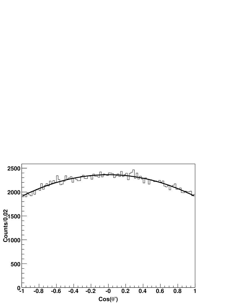
Figure 127: Generator-level angular distribution for $D$ in $D^{*}\rightarrow{D}{\gamma}$ for $D^{*}\bar{D}^{*}$ events. $\theta^{{}^{\prime}}$ is defined as the angle between the $D$ in the rest frame of the $D^{*}$ to that of the momentum vector of the $D^{*}$ in the lab.

Appendix F $e^{+}e^{-}\rightarrow\gamma^{*}\rightarrow{D^{*}\bar{D}^{*}}$, $D^{*}\rightarrow{D}{\pi}$

It has already been shown that the angular distribution, for production of $D^{*}$ with helicity of 1 is

$$\frac{dN}{d\cos\theta^{{}^{\prime}}}\propto(1-\cos^{2}\theta^{{}^{\prime}}).$$ (54)

Next, it can been shown that when $D^{*}$ has helicity of 0 the angular distribution is as follows:

$$\frac{dN}{d\cos\theta^{{}^{\prime}}}\propto|d^{1}_{00}(\theta{{}^{\prime}})|^{2}\propto\cos^{2}\theta^{{}^{\prime}}.$$ (55)

Again combining the three possible $D^{*}D^{*}$ helicity cases, with their associated amplitudes, yields the following angular distribution:

$$\frac{dN}{d\cos\theta^{{}^{\prime}}}=|B_{00}|^{2}\{(|A_{11}|^{2}+|A_{01}|^{2})+(|A_{00}|^{2}+|A_{01}|^{2}-|A_{11}|^{2})\cos^{2}\theta^{{}^{\prime}}\}.$$ (56)

Applying the same assumption as above, that is $A_{00}=A_{01}=A_{11}$, one arrives at the following distribution:

$$\frac{dN}{d\cos\theta^{{}^{\prime}}}\propto(1+\frac{1}{2}\cos^{2}\theta^{{}^{\prime}}).$$ (57)

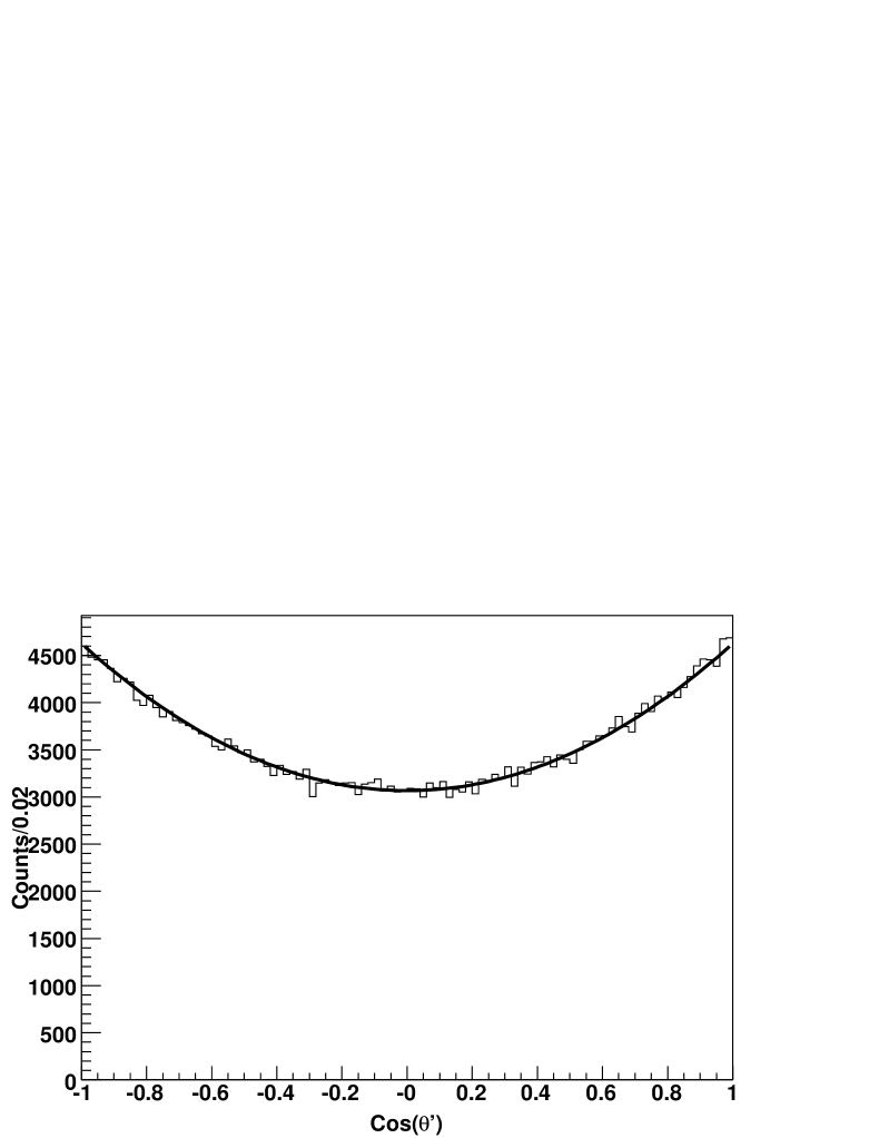
Figure 128: Generator-level angular distribution for $D$ in $D^{*}\rightarrow{D}{\pi^{0}}$ for $D^{*}\bar{D}^{*}$ events. $\theta^{{}^{\prime}}$ is defined as the angle between the $D$ in the rest frame of the $D^{*}$ to that of the momentum vector of the $D^{*}$ in the lab.

F.1 Momentum Distributions

F.1.1 Momentum Distributions of $D$-mesons in $e^{+}e^{-}\rightarrow\gamma^{*}\rightarrow{D^{*}\bar{D^{*}}}$ events

Notice that in all cases the angular distribution of a $D$ meson can be written as follows:

$$\frac{dN}{d\cos\theta}\propto 1+\alpha\cos^{2}(\theta)$$ (58)

where $\alpha$ is a function of the various helicity amplitudes present for the decay and event in question.

The momentum distribution for the decay $D$ mesons is as follows:

$$\frac{dN}{dP_{lab}}=\frac{dN}{d\cos\theta}\frac{d\cos\theta}{dP_{lab}}$$ (59)

The energy of the decay $D$ in the lab can be written as follow:

$${E_{lab}={\gamma}E^{o}+\beta{\gamma}P^{o}\cos(\theta)}$$ (60)

thus one gets, using $P_{lab}^{2}=E_{lab}^{2}-M^{2}$, the following expression:

$$\cos(\theta)=\frac{\sqrt{P^{2}_{lab}+M^{2}}-{\gamma}E^{o}}{\beta\gamma{P^{0}}}$$ (61)

and so:

$$\frac{d\cos(\theta)}{dP_{lab}}=\frac{P_{lab}}{\beta\gamma{P^{o}}\sqrt{P^{2}_{lab}+M^{2}}}$$ (62)

with $\beta\gamma=\frac{P_{D^{*}}}{M_{D^{*}}}$, $\gamma=\frac{E_{D^{*}}}{M_{D^{*}}}$, and $E^{o}=\frac{M_{D^{*}}^{2}+M_{X}^{2}-M^{2}}{2M_{D^{*}}}$, where $M$ and $M_{X}$ are the mass of the daugther $D$ and other particle (either a photon or pion) present in the decay, respectively. Therefore:

$$\frac{dN}{dP_{lab}}=\frac{P_{lab}}{\beta\gamma{P^{o}}\sqrt{P^{2}_{lab}+M^{2}}}\{1+\alpha\{\frac{\sqrt{P_{lab}^{2}+M^{2}}-\gamma{E^{o}}}{\beta\gamma{P}^{o}}\}^{2}\}$$ (63)

It is easily seen in the above expression the role that the angular distribution, indicted by the parameter $\alpha$, has on the momentum distribution. Examples of two cases, at $E=4030~{}$MeV, are shown in Figs. 129-130.

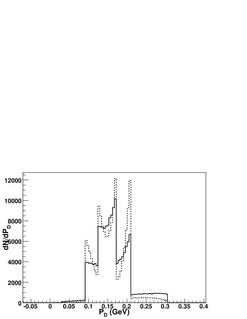
Figure 129: Momentum distribution for $D^{0}$ in $D^{*}D^{*}$ events. The different histograms correspond to different helicity amplitudes, and therefore different values for $\alpha$ in Eq. 63. The solid histogram has $\alpha=0.65$ and $\alpha=-0.24$ for the pion and gamma decay respectively. The dashed histogram has $\alpha=5.0$ and $\alpha=-0.71$ for the pion and gamma decay respectively.

Figure 130: This has the same parameters and values as Fig. 129 but has been convoluted with a gaussian of 10 MeV to account for detector resolution. This distribution should be compared to Fig. 95.

Appendix G Complete Derivation of $e^{+}e^{-}\rightarrow\gamma^{*}\rightarrow{D^{*}\bar{D}}$, $D^{*}\rightarrow{D}{\gamma}$

To help curb confusion let us define $e^{+}e^{-}\rightarrow\gamma^{*}\rightarrow{D^{*}\bar{D}}$, $D^{*}\rightarrow{D}{\gamma}$ as $\gamma^{*}\rightarrow 12$ and $1\rightarrow 34$ and define $A_{\lambda_{1}\lambda_{2}}$ to be the helicity amplitudes for $\gamma^{*}\rightarrow 12$ and $B_{\lambda_{3}\lambda_{4}}$ to be the helicity amplitudes for $1\rightarrow 34$. Therefore

$$A(M_{\gamma},\lambda_{1},\lambda_{2},\lambda_{3},\lambda_{4})=\sum_{\lambda_{1}}D^{1}_{\lambda_{1}\lambda^{\prime}}D^{1}_{M_{\gamma}\lambda}B_{\lambda_{3}\lambda_{4}}A_{\lambda_{1}\lambda_{2}}$$ (64)

where $\lambda^{\prime}=\lambda_{3}-\lambda_{4}$ and $\lambda=\lambda_{1}-\lambda_{2}$ and since $\lambda_{2}=\lambda_{4}=0$, $\lambda^{\prime}=\lambda_{3}$ and $\lambda=\lambda_{1}$ therefore:

$$A(M_{\gamma},\lambda_{1},0,\lambda_{3},0)=D^{1}_{0\lambda_{4}}D^{1}_{M_{\gamma}0}B_{0\lambda_{4}}A_{00}+$$

$$D^{1}_{1\lambda_{4}}D^{1}_{M_{\gamma}1}B_{0\lambda_{4}}A_{10}+$$

$$D^{1}_{-1\lambda_{4}}D^{1}_{M_{\gamma}-1}B_{0\lambda_{4}}A_{-10}$$ (65)

By Eq. 43 and the $J^{P}$ quantum numbers of the reaction, it is seen that party conservation requires $A_{00}=-A_{00}$ and $A_{10}=-A_{-10}$. Therefore, $A_{00}$ must be set to zero and so the $D^{*}$ will always be produced with helicity of $\lambda=\pm 1$. So:

$$A(M_{\gamma},\lambda_{1},0,\lambda_{3},0)=B_{0\lambda_{4}}A_{10}(D^{1}_{1\lambda_{4}}D^{1}_{M_{\gamma}1}-D^{1}_{-1\lambda_{4}}D^{1}_{M_{\gamma}-1})$$ (66)

The angular distribution is therefore:

$$\frac{dN}{d\Omega}=\sum_{M_{\gamma}}\sum_{\lambda_{4}}|A(M_{\gamma},\lambda_{1},0,\lambda_{3},0)|^{2}$$

$$=\sum_{M_{\gamma}}\sum_{\lambda_{4}}|A_{10}|^{2}|B_{0\lambda_{4}}|^{2}|D^{1}_{1\lambda_{4}}D^{1}_{M_{\gamma}1}-D^{1}_{-1\lambda_{4}}D^{1}_{M_{\gamma}-1}|^{2}$$ (67)

where $D^{1}_{M_{\gamma}1}=e^{-iM_{\gamma}\phi}d^{1}_{M_{\gamma}1}(\theta)e^{i\phi}$, $D^{1}_{M_{\gamma}-1}=e^{-iM_{\gamma}\phi}d^{1}_{M_{\gamma}-1}(\theta)e^{-i\phi}$,

$D^{1}_{1\lambda_{4}}=e^{-i\phi_{4}}d^{1}_{1\lambda_{4}}(\theta_{4})e^{i\lambda_{4}\phi_{4}}$ and $D^{1}_{-1\lambda_{4}}=e^{i\phi_{4}}d^{1}_{-1\lambda_{4}}(\theta_{4})e^{i\lambda_{4}\phi_{4}}$ where $\theta$ is defined as the angle between the $D^{*}$ and the beam axis and $\theta_{4}$ is defined as the angle between the $D$ in the rest frame of the $D^{*}$ to that of the momentum vector of the $D^{*}$ in the lab. By substitution of the $D$ functions one arrives at:

$$\frac{dN}{d\Omega}=\sum_{M_{\gamma}}\sum_{\lambda_{4}}|A_{10}|^{2}|B_{0\lambda_{4}}|^{2}(|d^{1}_{1\lambda_{4}}(\theta_{4})d^{1}_{M_{\gamma}1}(\theta)|^{2}+$$

$$|d^{1}_{-1\lambda_{4}}(\theta_{4})d^{1}_{M_{\gamma}-1}(\theta)|^{2}$$

$$-(d^{1}_{1\lambda_{4}}(\theta_{4})d^{1}_{M_{\gamma}1}(\theta)d^{1}_{-1\lambda_{4}}(\theta_{4})d^{1}_{M_{\gamma}-1}(\theta))2\cos(2\delta\phi))$$ (68)

where $\delta\phi=\phi_{4}-\phi$. Next, we sum over $\lambda_{4}$ where $\lambda_{4}=\pm 1$ since it represents a photon for the present case. Therefore $|B_{01}|^{2}=|B_{0-1}|^{2}$ meaning:

$$\frac{dN}{d\Omega}=|A_{10}|^{2}|B_{01}|^{2}(|d^{1}_{11}(\theta_{4})d^{1}_{M_{\gamma}1}(\theta)|^{2}+$$

$$|d^{1}_{-11}(\theta_{4})d^{1}_{M_{\gamma}-1}(\theta)|^{2}$$

$$-(d^{1}_{11}(\theta_{4})d^{1}_{M_{\gamma}1}(\theta)d^{1}_{-11}(\theta_{4})d^{1}_{M_{\gamma}-1}(\theta))2\cos(2\delta\phi)+$$

$$|d^{1}_{1-1}(\theta_{4})d^{1}_{M_{\gamma}1}(\theta)|^{2}+$$

$$|d^{1}_{-1-1}(\theta_{4})d^{1}_{M_{\gamma}-1}(\theta)|^{2}$$

$$-(d^{1}_{1-1}(\theta_{4})d^{1}_{M_{\gamma}1}(\theta)d^{1}_{-1-1}(\theta_{4})d^{1}_{M_{\gamma}-1}(\theta))2\cos(2\delta\phi))$$ (69)

again since we are not concerned by overall constants we set $M_{\gamma}=1$ and using the fact that $d^{1}_{11}=d^{1}_{-1-1}=\frac{1+\cos\theta}{2}$ and $d^{1}_{1-1}=d^{1}_{-11}=\frac{1-\cos\theta}{2}$ one arrives at the following:

$$\frac{dN}{d\Omega}\propto|A_{10}|^{2}|B_{01}|^{2}((1+\cos^{2}\theta_{4})(1+\cos^{2}\theta)+\sin^{2}\theta\sin^{2}\theta_{4}\cos(2\delta\phi))$$ (70)

therefore by integrating over the azimuthal angle, the $D^{*}$ has a $(1+\cos^{2}\theta)$ distribution with respect to the beam axis. In addition, one sees that the $D$, in $D^{*}\rightarrow{D}{\gamma},$will have a $(1+\cos^{2}\theta_{4})$ distribution in the rest frame of the $D^{*}$.

In repeating the above for $D^{*}\rightarrow{D}{\pi}$, that is setting $\lambda_{4}=0$, one arrives at:

$$\frac{dN}{d\Omega}\propto|A_{10}|^{2}|B_{00}|^{2}((1+\cos^{2}\theta)+\sin^{2}\theta\cos(2\delta\phi))\sin^{2}\theta_{4}$$ (71)

therefore one sees that this time the $D$, in $D^{*}\rightarrow{D}{\pi}$, will have a $\sin^{2}\theta_{4}$ distribution in the rest frame of the $D^{*}$. Also, it is clear that there is also azimuthal angular dependence present.

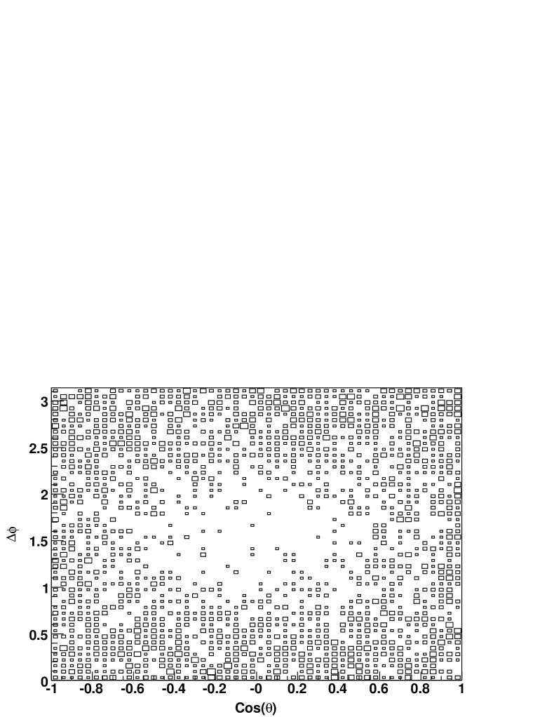
Figure 131: Generator level scatter plot showing the expected $\phi$ dependence for $e^{+}e^{-}\rightarrow\gamma^{*}\rightarrow{D^{*}\bar{D}}$ where $D^{*}\rightarrow{D}{\pi}$.

Chapter Results of Angular Distributions
of $D^{*}$ in $D^{*}\bar{D}^{*}$ Events

Appendix H $e^{+}e^{-}\rightarrow\gamma^{*}\rightarrow{D^{*}\bar{D}^{*}}$

The method used to reconstruct $D^{*}$ in $D^{*}\bar{D}^{*}$ events is to first find $D$ mesons that populate the appropriate region in $M_{\rm{bc}}$, see Table 12. After doing so, a pion, either charged or neutral, is added to the $D$ and a cut applied to $\Delta{\rm{M}}=|{\rm{M}}_{D^{*}}-{\rm{M}}_{D}|$ to purify the sample. For this study only $D^{*0}\rightarrow{D^{0}\pi^{0}}$ with $D^{0}\rightarrow{K^{-}}{\pi^{+}}$ and $D^{*+}\rightarrow{D^{+}\pi^{0}}$ with $D^{+}\rightarrow{K^{-}}{\pi^{+}}\pi^{+}$ are used. These $D$ modes represent the cleanest modes available and the $\pi^{0}$ decay modes for $D^{*}$ have an efficiency that is flat as a function of $\cos\theta$, which is not the case of the charged pion because of the opening angle in the $D^{*+}$ decays.

This method was first applied to Monte-Carlo and in addition to looking at $D^{*}$ in $D^{*}\bar{D}^{*}$ we also looked at $D$ in $D\bar{D}$ since its angular distribution is well-known and therefore used as a control. The MC results for $\alpha$, where $\alpha$ is defined in the general formula $1+\alpha\cos^{2}\theta$, as a function of center-of-mass energy is shown in Fig. 132, where the solid black lines correspond to the MC input value. The data result of $\alpha$ as a function of center-of-mass energy is shown in Fig. 133 where the red and blue lines correspond to the average value for $D^{0}\rightarrow{K^{-}}{\pi^{+}}$ and $D^{+}\rightarrow{K^{-}}{\pi^{+}}\pi^{+}$ respectively. In both cases the top plot presents the results of $D$ in $D\bar{D}$ and the bottom plot of $D^{*}$ in $D^{*}\bar{D}^{*}$. Lastly, $\theta$ is defined as the angle between the $D$ or $D^{*}$ momentum vector and the beam axis, its polar angle.

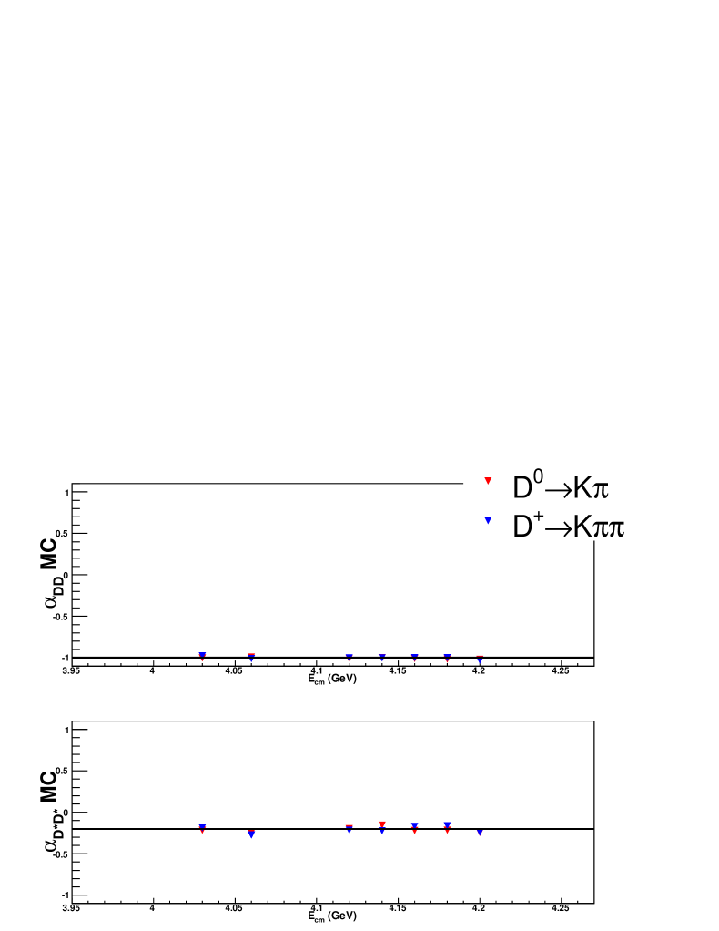
Figure 132: $\alpha$, defined in $1+\alpha\cos^{2}\theta$, as a function of center-of-mass energy from MC. The solid black lines correspond to the MC input value. Top plot presents the results of $D$ in $D\bar{D}$ and the bottom plot of $D^{*}$ in $D^{*}\bar{D}^{*}$.

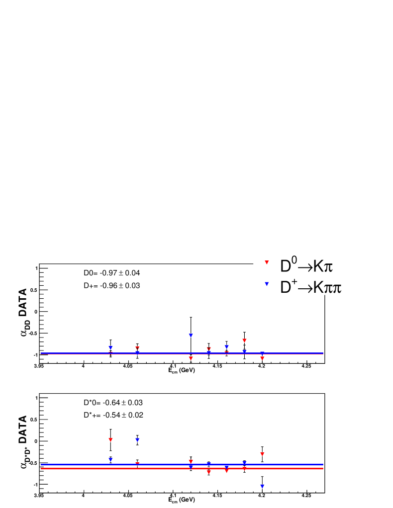
Figure 133: $\alpha$, defined in $1+\alpha\cos^{2}\theta$, as a function of center-of-mass energy from Data. The red and blue lines correspond to the average value for $D^{0}\rightarrow{K^{-}}{\pi^{+}}$ and $D^{+}\rightarrow{K^{-}}{\pi^{+}}\pi^{+}$ respectively. Top plot presents the results of $D$ in $D\bar{D}$ and the bottom plot of $D^{*}$ in $D^{*}\bar{D}^{*}$.

To help in our understanding it is beneficial to translate the helicity amplitudes into partial wave amplitudes using the Jacob-Wick Transformation:

$$A_{\lambda_{D_{1}^{*}}\lambda_{D_{2}^{*}}}=\sum_{{\rm{LS}}}\sqrt{\frac{2{\rm{L}}+1}{2{\rm{J}}+1}}({\rm{L}}0,S(\lambda_{D_{1}^{*}}-\lambda_{D_{2}^{*}})|J(\lambda_{D_{1}^{*}}-\lambda_{D_{2}^{*}}))$$

$$(s_{D_{1}^{*}}\lambda_{D_{1}^{*}},s_{D_{2}^{*}}-\lambda_{D_{2}^{*}}|S(\lambda_{D_{1}^{*}}-\lambda_{D_{2}^{*}})){\rm{M(L,S)}}$$ (72)

where $(Sm_{s},Tm_{t}|Jm_{j})$ correspond to Clebsh-Gordon coefficients. Either representation is valid, however, the Partial Wave representation is somewhat more intuitive since it is written in terms of orbital angular momentum and spin. For the case at hand, $e^{+}e^{-}\rightarrow{D^{*}D^{*}}$, there are three independent partial wave amplitudes, $M(1,0)$, $M(1,2)$, and $M(3,2)$, analogous to the three helicity amplitudes. By using Eq. H the following relations are obtained:

$$A_{00}=-\sqrt{\frac{1}{3}}M(1,0)-\sqrt{\frac{4}{15}}M(1,2)+\sqrt{\frac{2}{5}}M(3,2)$$ (73)

$$A_{10}=-\sqrt{\frac{3}{20}}M(1,2)-\sqrt{\frac{1}{10}}M(3,2)$$ (74)

$$A_{11}=\sqrt{\frac{1}{3}}M(1,0)-\sqrt{\frac{1}{15}}M(1,2)+\sqrt{\frac{1}{10}}M(3,2)$$ (75)

Since in Eq. 48 the amplitudes are always in terms of the modulus square Eqs. 73-75 are more useful if written as follows:

$$|A_{00}|^{2}=\frac{1}{3}|M(1,0)|^{2}+\frac{4}{15}|M(1,2)|^{2}+\frac{2}{5}|M(3,2)|^{2}+$$

$$4\sqrt{\frac{1}{45}}|M(1,2)||M(1,0)|\cos\phi_{M_{12}M_{10}}-$$

$$2\sqrt{\frac{2}{15}}|M(1,0)||M(3,2)|\cos\phi_{M_{10}M_{32}}-$$

$$\frac{4}{5}\sqrt{\frac{2}{3}}|M(1,2)||M(3,2)|\cos\phi_{M_{12}M_{32}}$$ (76)

$$|A_{10}|^{2}=\frac{3}{20}|M(1,2)|^{2}+\frac{1}{10}|M(3,2)|^{2}+$$

$$\frac{1}{5}\sqrt{\frac{3}{2}}|M(1,2)||M(3,2)|\cos\phi_{M_{12}M_{32}}$$ (77)

$$|A_{11}|^{2}=\frac{1}{3}|M(1,0)|^{2}+\frac{1}{15}|M(1,2)|^{2}+\frac{1}{10}|M(3,2)|^{2}$$

$$-2\sqrt{\frac{1}{45}}|M(1,2)||M(1,0)|\cos\phi_{M_{12}M_{10}}$$

$$+2\sqrt{\frac{1}{30}}|M(1,0)||M(3,2)|\cos\phi_{M_{10}M_{32}}$$

$$-\frac{2}{5}\sqrt{\frac{1}{6}}|M(1,2)||M(3,2)|\cos\phi_{M_{12}M_{32}}$$ (78)

where $\phi_{M_{12}M_{10}}$ is the $\arg(M(1,2)M^{*}(1,0))$, $\phi_{M_{10}M_{32}}$ is the $\arg(M(1,0)M^{*}(3,2))$, and $\phi_{M_{12}M_{32}}$ is the $\arg(M(1,2)M^{*}(3,2))$. By applying the above equations to Eq. 48 one arrives at:

$$\frac{dN}{d\cos{\theta}}=\frac{3}{2}|M(1,0)|^{2}(1-z)+\frac{21}{20}|M(1,2)|^{2}(1-\frac{1}{7}z)+$$

$$\frac{6}{5}|M(2,3)|^{2}(1-\frac{1}{2}z)-\frac{3}{5}\sqrt{\frac{3}{2}}|M(1,2)||M(3,2)|(3z-1)\cos\phi_{M_{12}M_{32}}$$ (79)

where $z=\cos(\theta)^{2}$. Now the $L=3$ F-wave amplitude contains two extra powers of the center-of-mass momentum, relative to a P-wave, and therefore should be small near the threshold [73]. By setting $|M(3,2)|=0$ in Eq. H one arrives at the following:

$$\frac{dN}{d\cos{\theta}}=\frac{3}{2}|M(1,0)|^{2}(1-z)+\frac{21}{20}|M(1,2)|^{2}(1-\frac{1}{7}z).$$ (80)

Notice that this distribution is independent of any phase. By setting $|M(1,2)|^{2}=|M(1,0)|^{2}$ we get:

$$\frac{dN}{d\cos{\theta}}\propto 1-\frac{11}{17}\cos^{2}\theta=1-0.65\cos^{2}\theta.$$ (81)

It is seen that the translation to the partial wave basis is only beneficial for the case near threshold and adds another unknown to our equation at all other energies. Therefore, we will stick to the helicity basis and will rewrite Eq. 48 as follows:

$$\frac{dN}{d\cos{\theta}}\propto 1+\alpha\cos^{2}\theta$$ (82)

where $\alpha$ is defined as:

$$\alpha=\frac{2|A_{01}|^{2}-2|A_{11}|^{2}-|A_{00}|^{2}}{2|A_{01}|^{2}+2|A_{11}|^{2}+|A_{00}|^{2}}=\frac{1-2b}{1+2b}$$ (83)

with $b=\frac{|A_{00}|^{2}+2|A_{11}|^{2}}{4|A_{01}|^{2}}$. The best fit to the $D^{*}$ production distribution is shown in Fig. 134.

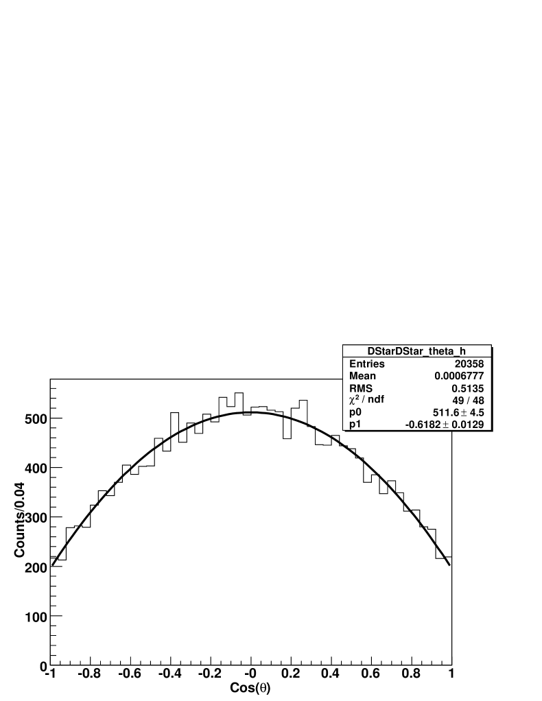
Figure 134: Plot of the production angle for $D^{*}$ in $D^{*}D^{*}$ events for data at 4170 MeV. The solid line shows the best fit to the data using the fit function $1+\alpha\cos^{2}(\theta)$, where $\theta$ is the production angle. Based on the fit $\alpha=-0.62\pm 0.01$.

Appendix I $e^{+}e^{-}\rightarrow\gamma^{*}\rightarrow{D^{*}\bar{D}^{*}}$, $D^{*}\rightarrow{D}{\pi}$

It has been shown earlier that the angular distribution for $D$-mesons in $D^{*}\rightarrow{D}{\pi}$ decays is as follows:

$$\frac{dN}{d\cos\theta^{{}^{\prime}}}=|B_{00}|^{2}\{(|A_{11}|^{2}+|A_{01}|^{2})+(|A_{00}|^{2}+|A_{01}|^{2}-|A_{11}|^{2})\cos^{2}\theta^{{}^{\prime}}\}.$$ (84)

where $\theta^{{}^{\prime}}$ is defined as the angle between the $D$ in the rest frame of the $D^{*}$ and the momentum vector of the $D^{*}$ in the lab and $B_{00}$ is the helicity amplitude for $D^{*}\rightarrow{D}{\pi}$. By substituting Eqs. H-H one arrives at:

$$\frac{dN}{d\cos\theta^{{}^{\prime}}}=\frac{1}{3}|M(1,0)|^{2}+\frac{21}{60}|M(1,2)|^{2}(z+\frac{13}{21})+\frac{1}{5}|M(3,2)|^{2}(1+2z)$$

$$+2\sqrt{\frac{1}{5}}|M(1,2)||M(1,0)|\cos\phi_{M_{12}M_{10}}(z-\frac{1}{3})$$

$$+2\sqrt{\frac{1}{30}}|M(1,0)||M(3,2)|\cos\phi_{M_{10}M_{32}}(1-3z)$$

$$+\frac{1}{5}\sqrt{\frac{1}{6}}|M(1,2)||M(3,2)|\cos\phi_{M_{12}M_{32}}(1-3z)$$ (85)

Now assuming that the $D$-mesons are produced close to threshold, that is $L=3$ F-wave amplitude is small, we can set $|M(3,2)|=0$ in Eq. I and arrive at the following:

$$\frac{dN}{d\cos\theta^{{}^{\prime}}}=\frac{13}{60}|M(1,2)|^{2}+\frac{1}{3}|M(1,0)|^{2}-2\sqrt{\frac{1}{45}}|M(1,2)||M(1,0)|\cos\phi_{02}$$

$$+(\frac{21}{60}|M(1,2)|^{2}+6\sqrt{\frac{1}{45}}|M(1,2)||M(1,0)|\cos\phi_{02})\cos^{2}\theta^{{}^{\prime}}$$ (86)

Notice that this distribution is NOT independent of $\phi_{M_{10}M_{12}}$. By setting $|M(1,2)|^{2}=|M(1,0)|^{2}$ and $\phi_{M_{10}M_{12}}=\frac{\pi}{2}$ we get:

$$\frac{dN}{d\cos\theta^{{}^{\prime}}}\propto 1+\frac{21}{33}\cos^{2}\theta^{{}^{\prime}}=1+0.64\cos^{2}\theta^{{}^{\prime}}$$ (87)

and with $\phi_{M_{10}M_{12}}=0$ we get:

$$\frac{dN}{d\cos\theta^{{}^{\prime}}}\propto 1+\frac{\frac{21}{60}+6\sqrt{\frac{1}{45}}}{\frac{33}{60}-2\sqrt{\frac{1}{45}}}\cos^{2}\theta^{{}^{\prime}}=1+5.0\cos^{2}\theta^{{}^{\prime}}.$$ (88)

showing that, even in the case where $|M(3,2)|=0$, a wide range of angular distributions are allowed.

Again, we see that transforming to the partial wave basis is only useful near threshold, therefore we will stick to the helicity basis and will rewrite Eq. 84 as follows:

$$\frac{dN}{d\cos{\theta^{{}^{\prime}}}}\propto 1+\alpha^{{}^{\prime}}\cos^{2}\theta^{{}^{\prime}}$$ (89)

where $\alpha^{{}^{\prime}}$ is defined as:

$$\alpha^{{}^{\prime}}=\frac{|A_{00}|^{2}+|A_{01}|^{2}-|A_{11}|^{2}}{|A_{11}|^{2}+|A_{01}|^{2}}=\frac{1+\frac{1+a}{4b}-\frac{a}{2}}{\frac{a}{2}+\frac{1+a}{4b}}$$ (90)

with $a=\frac{2|A_{11}|^{2}}{|A_{00}|^{2}}$. Using Eq. 63 convoluted with a Crystal Ball resolution function, the width of the resolution function was chosen to be $\sim 8.5$ MeV which is based on MC $D\bar{D}$ events generated with a momentum of 500 MeV/$c$, one can obtain the coefficient $\alpha^{{}^{\prime}}$. A Crystal Ball function Eq. 91 is used in an attempt to account for the ISR effects which are present. The Crystal Ball function is defined as follows:

$$f(x;\alpha,n,\bar{x},\sigma)=N\begin{cases}e^{-\frac{(x-\bar{x})^{2}}{2\sigma^{2}}},&{\rm{for}}\frac{x-\bar{x}}{\sigma}>-~{}\alpha\\ A\cdot(B-\frac{x-\bar{x}}{\sigma})^{-n},&{\rm{for}}\frac{x-\bar{x}}{\sigma}\leq{-~{}}\alpha\end{cases}$$ (91)

where $A=(\frac{n}{\alpha})^{n}\cdot{e}^{-\frac{|\alpha|^{2}}{2}}$, $B=\frac{n}{|\alpha|}-|\alpha|$ and N, $\alpha$, $n$, $\bar{x}$, $\sigma$ are the fit parameters which are determined by the generated MC and then fixed in the convolution. The fit to the $D$ momentum spectrum is shown in Fig. 135.

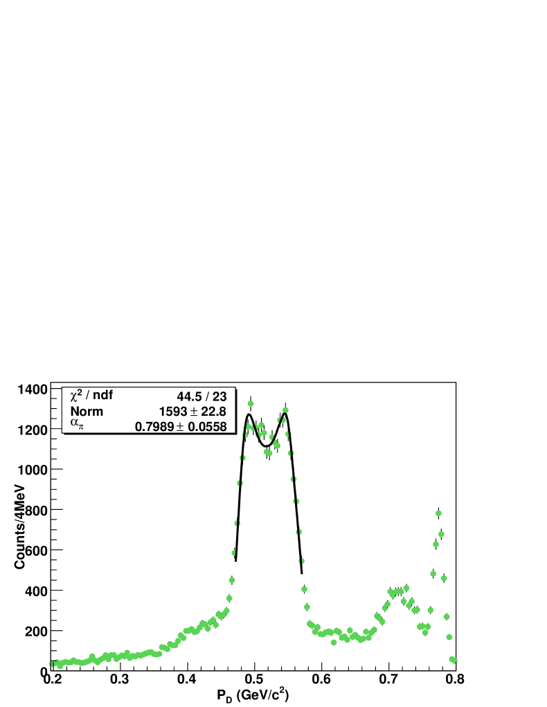
Figure 135: The $D^{0}$ momentum spectrum. The points with error bars is the data collected at 4170 MeV and the solid line is the best fit result. The fit function consisted of Eq. 63 convoluted with a gaussian resolution function. The result of the fit yields $\alpha^{{}^{\prime}}=0.80\pm 0.06$.

Using the definitions of $\alpha$ and $\alpha^{{}^{\prime}}$ along with the normalization condition that $|A_{00}|^{2}+4|A_{10}|^{2}+2|A_{11}|=1$, one is able to arrive at the following:

$$|A_{00}|^{2}=0.314\pm 0.009$$ (92)

$$|A_{10}|^{2}=0.080\pm 0.003$$ (93)

$$|A_{11}|^{2}=0.183\pm 0.003$$ (94)

Since in the equations Eq. 48 and 84 the helicity amplitudes enter as the modulus squared, one needs not to worry about the relative phase or the sign of the amplitudes. Therefore, in order to generate the observed angular distributions for $D^{*}D^{*}$ events using EVTGEN’s Helicity Amplitude Model (HELAMP) one needs the following:

D*0 anti-D*0 HELAMP 0.43 0.0 0.28 0.0 0.28 0.0 0.56 0.0 0.28 0.0 0.28 0.0 0.43 0.0;

Comparison between the data and a generated MC sample, using the above HELAMP model, is shown in Figs. 136 and 137.

Figure 136: Plot of the production angle for $D^{*}$ at 4170 MeV. Data is shown along with a generated MC sample using the helicity amplitudes described in the text.

Figure 137: Plot of the angle between the $D$ in the rest frame of the $D^{*}$ and the momentum of the $D^{*}$ in the lab for $D^{*}D^{*}$ events at $4170$ MeV. Data is shown along with a generated MC sample using the helicity amplitudes described in the text.

References

- [1] M. Gell-Mann, Phys. Lett. 8, 214 (1964); G. Zweig, CERN Reports Nos. Th 401 and Th 412, 1964 (unpublished).
- [2] S. Eidelman et al. , (Particle Data Group Collaboration), Phys. Lett., B592 1 (2004).
- [3] W. O. Greenberg, Phys. Rev. Lett. 13, 598 (1964). The terminology of “color” did not enter till the 1970s.
- [4] D. J. Gross and F. Wilczek Phys. Rev. Lett., 30 1343 (1973). H. D. Politzer Phys. Rev. Lett., 30 1346 (1973).
- [5] B. J. Bjoken and S. .L Glashow, Phys. Lett., 11 255 (1964).
- [6] S. L. Glashow, J. Iliopoupos, and L. Maiani, Phys. Rev., D2, 1285 (1970).
- [7] D. Griffiths, “Introduction to Elementary Particles”, John Wiley & Sons, Inc., New York (1987).
- [8] N. Cabibbo, Phys. Rev. Lett, 10, 531 (1963).
- [9] M. Kobayashi and T. Maskawa, Prog. Theor. Phys., 49, 652 (1973).
- [10] M. K. Gaillard and B. W. Lee, Phys. Rev., D10, 897 (1974).
- [11] S. Okubo, Phys. Lett., 5, 165 (1966). G. Zweig CERN preprint TH 401 and TH 412 (1964). J. Iizuka Prog. Theor. Phys. Suppl., 37, 21 (1966).
- [12] M. K. Gaillard, B. W. Lee, and J. L. Rosner, Rev. Mod. Phys. 47, 277 (1977).
- [13] G. Goldhaber et al. , Phys. Rev. Lett, 37, 255 (1976). I. Peruzzi et al. , Phys. Rev. Lett, 37, 569 (1976).
- [14] G. Goldhaber et al. , SLAC-PUB-1973 and LBL-6467 (1977).
- [15] A. Chen et al. , Phys. Rev. Lett. 51, 634 (1983).
- [16] S. Stone, [HEPPH-0010295] (2000).
- [17] B. Aubert et al. [BABAR Collaboration], Phys. Rev. Lett. 95, 142001 (2005).
- [18] J. Z. Bai, [HEPEX-0102003] (2001). J. Z. Bai et al. , Phys. Rev. Lett. 88, 101802 (2002).
- [19] J. Z. Bai et al. , Phys. Rev., D52, 3781 (1995).
- [20] J. Adler et al. , Phys. Rev. Lett., 63 1211 (1989).
- [21] G. Blaylock et al. , Phys. Rev. Lett., 58 2171 (1987).
- [22] M. Piccolo et al. , SLAC-PUB-1978 and LBL-6489 (1977).
- [23] M. Piccolo et al. , SLAC-PUB-2323 and LBL-7935 (1979).
- [24] M. W. Coles et al. , SLAC-PUB-2916 and LBL-14402 (1982).
- [25] J. Z. Bai et al. , Phys. Rev., D62, 012002 (2000).
- [26] A. Rujula, H.Georgi, and S. L. Glashow, Phys. Rev. Lett., 37, 398 (1976).
- [27] E. Eichten et al. , Phys. Rev., D21, 203 (1980).
- [28] T. Barnes, “Higher Charmonium,” [hep-ph/0412057] (2004).
- [29] L. Micu, Nucl. Phys. B10, 521 (1969).
- [30] R. .A. Briere et al. , “CLEO-c and CESR-c: A New Frontier of Weak and Strong Interactions”, CLNS 01/1742 (2001).
- [31] H. Wiedemann, “Particle Accelerator Physics”, Springer-Verlag, New York, NY (1993).
- [32] D. Rice (for the CESR staff), “CESR-c Configuration and Performance”, presented at miniMAC, Cornell University, Ithaca, NY, USA, July 22-23, 2005.
- [33] CLEO Collaboration internal document, Véronique Boisvert, CBX 00-70.
- [34] CLEO Collaboration internal document, XXXX, CBX 05-10.
- [35] D. Peterson , Nucl. Instrum. Meth. A478, 142 (2002).
- [36] M. Artuso , Nucl. Instrum. Meth. A554, 147 (2005).
- [37] M. Artuso , Nucl. Instrum. Meth. A441, 374 (2000).
- [38] Y. Kubota , Nucl. Instrum. Meth. A320, 66 (1992).
- [39] D. Bortoletto , Nucl. Instrum. Meth. A320, 114 (1992).
- [40] CLEO Collaboration internal document, Robert Kutschke and Anders Ryd, CBX 96-20.
- [41] R. M. Hans, C. L. Plager, M. A. Selen, and M. J. Haney, IEEE Trans. Nucl. Sci. 48, 552 (2001).
- [42] G. D. Gollin, J. A. Ernst, J. B. Williams, R. M. Hans, and M. J. Haney, IEEE Trans. Nucl. Sci. 48, 547 (2001).
- [43] M. A. Selen, R. M. Hans, and M. J. Haney, IEEE Trans. Nucl. Sci. 48, 562 (2001).
- [44] N. E. Adams et al. , [hep-ex/0607079] (2006).
- [45] Q. He et al. [CLEO Collaboration], Phys. Rev. Lett. 95, 121801 (2005) [arXiv:hep-ex/0504003].
- [46] CLEO Collaboration internal document, D. Cassel et al. , CBX 05-8 (2005).
- [47] CLEO Collaboration internal document, R. Briere et al. , CBX 04-32 (2004).
- [48] H. Albrecht et al. [ARGUS Collaboration], Phys. Lett. B241, 278 (1990).
- [49] CLEO Collaboration internal document, H. Muramatsu and E. Thorndike, CBX 05-51 (2005).
- [50] CLEO Collaboration internal document, H. Muramatsu and E. Thorndike, CBX 05-65 (2005).
- [51] D. Besson et al. [CLEO Collaboration], Phys. Rev. Lett. 96, 092002 (2006).
- [52] C. M. Carloni Calame et al. , Nucl. Phys. Proc. Suppl. B 131, 48 (2004).
- [53] R. Kleiss and S. van der Marck, Nucl. Phys. B 342, 61 (1990).
- [54] S. Jadach, Z. Was, Comput.Phys.Commun. 36, 191 (1985);
- [55] CLEO Collaboration internal document, B. Heltsley and H. Mahlke, CBX 04-47 (2004).
- [56] E. A. Kureav and V. S. Fadin, Sov. J. Nucl. Phys. 41, 466 (1985).
- [57] A. Ryd et al. , BAD 522 V6 and EvtGen V00-10-22 (2003).
- [58] CLEO Collaboration internal document, S. Mehrabyan, B. Heltsley, CBX 05-10 (2005).
- [59] G. Bonneau and F. Martin, Nucl. Phys. B27, 381 (1971).
- [60] A. Osterfeld et al. SLAC-PUB-4160 (1986) (unpublished).
- [61] K. Abe et al. , [hep-ex/0608018] (2006).
- [62] B. Aubert et al. , Phys. Rev. D73, 012005 (2006).
- [63] B. Aubert et al. , [hep-ex/0607083] (2006).
- [64] R. Poling [hep-ph/0606016] (2006).
- [65] M. B. Voloshin [hep-ph/0602233] (2006).
- [66] S. Dubynskiy and M. B. Voloshin [hep-ex/0608179] (2006).
- [67] M. Artuso et al. , [hep-ex/0607074] (2006).
- [68] T.E. Coan et al. , Phys. Rev. Lett. 96, 162003 (2006).
- [69] Haibo Li (For BES-III Collaboration), [hep-ex/0605004] (2006).
- [70] J. D. Richman CALT-68-1148 (1984) (unpublished).
- [71] H. K. Nguyen et al. , Phys. Rev. Lett., 39 262 (1977).
- [72] R. Kutschke, “An Angular Distribution Cookbook”, (1996).
- [73] M. B. Voloshin, private communication.