On the importance of high redshift intergalactic voids

Abstract

We investigate the properties of one–dimensional flux “voids” (connected regions in the flux distribution above the mean flux level) by comparing hydrodynamical simulations of large cosmological volumes with a set of observed high–resolution spectra at $z\sim 2$. After addressing the effects of box size and resolution, we study how the void distribution changes when the most significant cosmological and astrophysical parameters are varied. We find that the void distribution in the flux is in excellent agreement with predictions of the standard $\Lambda$CDM cosmology, which also fits other flux statistics remarkably well. We then model the relation between flux voids and the corresponding one–dimensional gas density field along the line–of–sight and make a preliminary attempt to connect the one–dimensional properties of the gas density field to the three–dimensional dark matter distribution at the same redshift. This provides a framework that allows statistical interpretations of the void population at high redshift using observed quasar spectra, and eventually it will enable linking the void properties of the high–redshift universe with those at lower redshifts, which are better known.

1 Introduction

Over the past decade, properties of voids have been more widely investigated, using different observational probes and tracers (mainly in the local universe, see for example Hoyle & Vogeley (2004), Rojas et al. (2004), Goldberg et al. (2005), Rojas et al. (2005), Hoyle et al. (2005), Ceccarelli et al. (2006), Patiri et al. (2006a), Patiri et al. (2006b), Tikhonov & Karachentsev (2006)), and theoretical – analytical or numerical – models in the framework of the $\Lambda$ Cold Dark Matter ($\Lambda$CDM) concordance cosmology (e.g. Peebles (2001), Arbabi-Bidgoli & Müller (2002), Mathis & White (2002), Benson et al. (2003), Gottlöber et al. (2003), Sheth & van de Weygaert (2004), Goldberg & Vogeley (2004), Bolejko et al. (2005), Colberg et al. (2005), Padilla et al. (2005), Furlanetto & Piran (2006), Hoeft et al. (2006), Lee & Park (2006), Patiri et al. (2006c), Shandarin et al. (2006), D’Aloisio & Furlanetto (2007), Tully (2007), Park & Lee (2007), Brunino et al. (2007), van de Weygaert & Schaap (2007), Neyrinck (2007), Peebles (2007)).

The emerging picture is encouraging. On the one hand, some results appear to be somewhat hard to understand, such as the fact that galaxies observed at the edges of and in voids appear to be a fair sample of the whole galaxy population (the so-called ’void phenomenon’, Peebles (2001)), the fact that dwarf galaxies are not found in voids contrary to expectations from numerical simulations (e.g. Peebles (2007), or the cold spot observed in the Cosmic Microwave Background (CMB) data (Rudnick et al. (2007), Naselsky et al. (2007)). On the other hand, other observational results, such as those from the 2dF or SDSS galaxy redshift surveys, from studies of voids in quasar spectra, or the CMB spectrum (Caldwell & Stebbins (2007)), are in reasonably good agreement with theoretical predictions from numerical simulations of the standard $\Lambda$CDM cosmology. Linking the low–redshift properties of voids to those at higher redshifts offers the opportunity to constrain the void population over a significant fraction of cosmic time and to possibly find out more about voids, to ultimately understand their role in the context of cosmic structure formation.

Unfortunately, there are very few observables that constrain the population of voids at high redshift (see, however, D’Aloisio & Furlanetto (2007)). Here, we will use the Lyman-$\alpha$ forest as a tracer of voids in the high–redshift universe. The Lyman-$\alpha$ forest (e.g. Bi & Davidsen (1997)) has been shown to arise from the neutral hydrogen embedded in the mildly non–linear density fluctuations around mean density in the Intergalactic Medium (IGM), which faithfully traces the underlying dark–matter distribution at scales above the Jeans length. It is a powerful cosmological tool in the sense that it probes the dark matter power spectrum in a range of scales ($1$ to $80\,h^{-1}$ Mpc comoving) and redshifts ($z=$2–5.5) not probed by other observables. However, the observable is not the matter distribution itself but the flux: a one–dimensional quantity sensitive not only to cosmological but also to the astrophysical parameters that describe the IGM.

The so–called fluctuating Gunn–Peterson approximation (Gunn & Peterson, 1965) relates the observed flux to the IGM overdensity in a simple manner once the effects of peculiar velocities, thermal broadening, and noise properties are neglected:

$$F({\bf{x}},z)=\exp[-A(z)(1+\delta_{IGM}({\bf{x}},z))^{\beta}]\,,$$ (1)

with $\beta(z)\sim 2-0.7(\gamma(z)-1)$, $\gamma$ the parameter describing the power–law (’equation of state’) relation of the IGM, $T=T_{0}(z)((1+\delta_{IGM})^{\gamma-1}$, and $A(z)$ a constant of order unity which depends on the mean flux level, on the Ultra Violet Background (UVB) and on the IGM temperature at mean density. In practice, linking the flux to the density of the dark (or gaseous) matter requires the use of accurate hydrodynamical simulations that incorporate the relevant physical and dynamical processes. However, for approximate calculations equation (1), in conjunction with simple physical prescriptions of Lyman-$\alpha$ clouds (e.g. Schaye (2001)), can offer precious insights.

Provided the flux–density relation is accurately modelled, using the Lyman-$\alpha$ forest to check the properties of the population of voids in the matter distribution would avoid having to know the bias between galaxies and dark matter and would allow to sample over larger volumes the values of cosmological parameters that affect the void population. On the other hand, the fact that the flux information is one–dimensional requires non–trivial efforts to relate it to the three–dimensional (dark) matter density field. Motivated by huge amounts of new data of exquisite quality, we here present a first attempt in this direction. Note that in the early 1990s, before the new paradigm of the Lyman-$\alpha$ forest absorption was proposed, voids from the transmitted Lyman-$\alpha$ flux of QSO spectra were analysed, using discrete statistics on the lines, by several groups (e.g. Crotts (1987); Duncan et al. (1989); Ostriker et al. (1988); Dobrzycki & Bechtold (1991); Rauch et al. (1992)). These attempts, however, did not reach conclusive results due to small–number statistics. We defer to a future paper for a link between the observational properties outlined here and those at low redshift (e.g. Mathis & White (2002); Hoyle & Vogeley (2004)) and for a careful investigation of the absorber–galaxy relation (e.g. Stocke et al. (1995); McLin et al. (2002)).

This paper is organized as follows. In Section 2, we briefly describe the data set used. In Section 3 we present the hydrodynamical simulations. Section 4 contains the bulk of our analysis and the results, which are summarized in the conclusions in Section 5.

2 The data set

We use the set of 18 high signal–to–noise (S/N$>30$–$50$), high–resolution ($R\sim 45000$) quasar spectra taken with the VLT/UVES presented in (Kim et al., 2007). We regard these spectra as a state–of–the–art, high–resolution sample in the sense that many statistical properties of the transmitted flux (mean flux decrement, flux probability distribution function, and flux power and bispectrum) have been accurately investigated and interpreted by several authors from the same or from similar data sets (see, for example, McDonald et al. (2000), Kim et al. (2004), Jena et al. (2005), Viel et al. (2004b), Bolton et al. (2007)). More importantly, systematics effects such as metal contamination, noise and resolution properties, and continuum fitting errors have been extensively addressed. From the data set, we discard the four highest redshift QSOs, in order to have a more homogenous sample at a median $<z>=2.2$ and with a total redshift path $\Delta z=6.1$. The pixels contributing to the signal are in the wavelength range $3282$–$4643\,\AA$ while the wavelength ranges for each single QSO spectrum are reported in Kim et al. (2007). Both Damped Lyman-$\alpha$ systems and metal lines have been removed from this sample. The evolution of the effective optical depth derived from this data set, $\tau_{\rm eff}=-\ln<F>$, which – as we will see – is the main input needed to constrain and identify voids, has been widely discussed and compared with various other measurements (Kim et al., 2007).

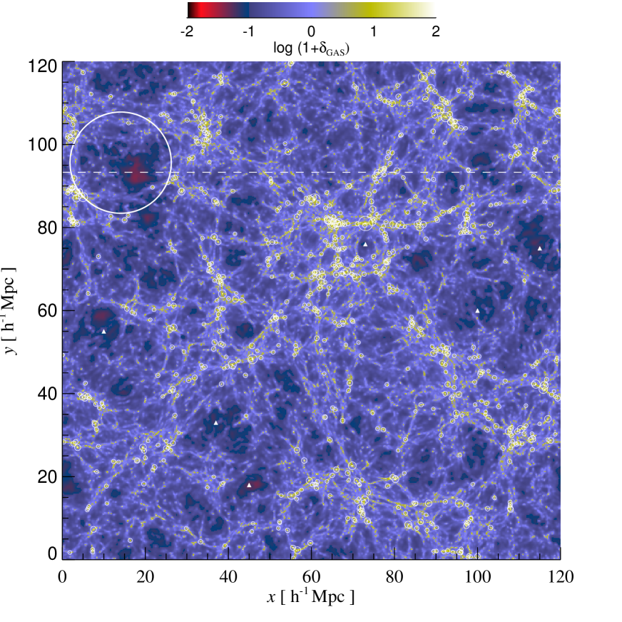
Figure 1: Slice of the projected gas density (thickness is 10 Mpc$/h$) from our reference $\Lambda$CDM hydrodynamical simulation at $z=2.2$. The presence of roughly spherical regions below the mean density of sizes of the order tens of Mpc is clear, denser environments at $\delta\sim 100$ tend to line up in filaments or could be found (more rarely) inside underdense regions (voids). A large underdense region is shown as a white thick circles, while haloes with total masses above $2\times 10^{11}M_{\odot}$, that trace the cosmic web, are represented by smaller white circles with radii proportional to their masses. The dashed line–of–sight will be analysed more closely in Section 4.4. Filled triangles indicate some underdense regions of different sizes: usually smaller voids are surrounded by many massive haloes, while larger ones have less haloes at their edges (with smaller masses).

3 The simulations

We use a set of simulations run with GADGET-2, a parallel tree Smoothed Particle Hydrodynamics (SPH) code that is based on the conservative ‘entropy-formulation’ of SPH (Springel, 2005). The simulations cover a cosmological volume (with periodic boundary conditions) filled with an equal number of dark matter and gas particles. Radiative cooling and heating processes were followed for a primordial mix of hydrogen and helium. We assume a mean UVB produced by quasars and galaxies as given by Haardt & Madau (1996), with helium heating rates multiplied by a factor $3.3$ in order to better fit observational constraints on the temperature evolution of the IGM. This background naturally gives $\Gamma_{12}\sim 1$ at the redshifts of interest here (Bolton et al., 2005). The star formation criterion very simply converts all gas particles whose temperature falls below $10^{5}$ K and whose density contrast is larger than 1000 into (collisionless) star particles (it has been shown that the star formation criterion has a negligible impact on flux statistics, see for example Viel et al. (2004) and Bolton et al. (2007)). More details of the simulations can be found in (Viel et al., 2004).

The cosmological model corresponds to the ‘fiducial’ $\Lambda$CDM Universe with $\Omega_{\rm m}=0.26,\ \Omega_{\Lambda}=0.74,\ \Omega_{\rm b}=0.0463$, $n_{s}=0.95$, and $H_{0}=72$ km s^-1 Mpc^-1 and $\sigma_{8}=0.85$ (the B2 series of Viel et al. (2004)). We use $2\times 400^{3}$ dark matter and gas particles in a volume of size $120\ h^{-1}$ Mpc box. For cross checks we also analyse smaller boxes of size $60,30,$ and $15\,h^{-1}$ Mpc. The gravitational softening was set to $15\,h^{-1}$ kpc in comoving units for all particles for the largest simulated volume and changes accordingly for the smaller volumes. In the following, the different simulations will be referred to by the tuple (comoving box size in Mpc$/h$,(no. gas particles)^1/3), so (120,400) denotes our fiducial simulation etc. (all the sizes reported in the rest of the paper will be in comoving units). In Figure 1 we show a two–dimensional slice of thickness 10 comoving Mpc$/h$ of the gas density for our reference simulation at $z=2.2$. Large regions whose gas density is below the mean are present and overdense regions separate them and give rise to the cosmic web. Occasionally denser regions of overdensity $\sim 100$ reside in the inner regions of voids, however their sizes are quite small and their impact parameter in the lines–of–sight to distant QSOs should be also relatively small. In Figure 1 we also overplot the haloes whose total mass is above $2\times 10^{11}M_{\odot}$ (white circles) and show some underdense regions of different sizes (filled triangles). Usually, the larger voids are surrounded by few and not very massive haloes that line up in filaments, while smaller voids, such as the one at $(x=77,y=73)$ Mpc$/h$ have more spherical shapes and have more massive haloes around them.

Note that some numerical efforts in order to simulate the intergalactic voids are required: on one side large volumes need to be simulated in order to sample the void distribution at large sizes, on the other side relatively high resolution is mandatory. In fact, with poor resolution the denser regions at the edge of voids are not properly resolved and will result in a smaller amount of neutral hydrogen and thereby less absorption: this will cause an overestimate of the void sizes.

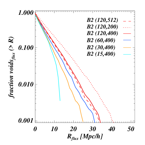
Figure 2: Box size and resolution effects at $z=2$ on the fraction of one–dimensional voids in the flux distribution (of size $R$ or larger), extracted from four different simulation volumes (120, 60, 30 and 15 $h^{-1}$ Mpc) and three different resolutions ($200^{3},400^{3},512^{3}$ gas particles). The flux has been smoothed with a 1D top–hat filter of size $1\,h^{-1}$ Mpc, which roughly corresponds to the Jeans length at this redshift. Spectra have been normalized to the same effective optical depth.

The parameters chosen here, including the thermal history of the IGM, are in reasonably good agreement with observational constraints and with recent results from CMB data, weak lensing and other data sets obtained from the Lyman-$\alpha$ forest (e.g. Viel et al. (2006), Lesgourgues et al. (2007)). The mock QSO spectra extracted from the simulations have the same resolution and noise properties as the observed ones, even though this will not affect our results. Here, for two reasons we consider only simulation snapshots at $z\sim 2$. First, the high–resolution data set has a median redshift $<z>=2.2$. Second, at these redshifts the UVB should be uniform, and the IGM’s equation–of–state is reasonably measured, leaving little room for ionization voids to be labelled as matter voids or for temperature fluctuations to strongly affect the Lyman-$\alpha$ forest properties (Shang et al., 2007). However, we caution that: $i)$ recent results from Bolton et al. (2007), based on the flux probability distribution function, seem to suggest that the thermal state of the IGM at $z<3$ could be more complex than expected; $ii)$ patchy HeII reionization at $z\sim 3.2$ could affect the uniformity of the UVB (e.g. Bolton et al. (2006); Faucher-Giguere et al. (2007)) and some effects at smaller redshifts might influence Lyman-$\alpha$ opacity.

4 Results

4.1 The 1D flux void distribution

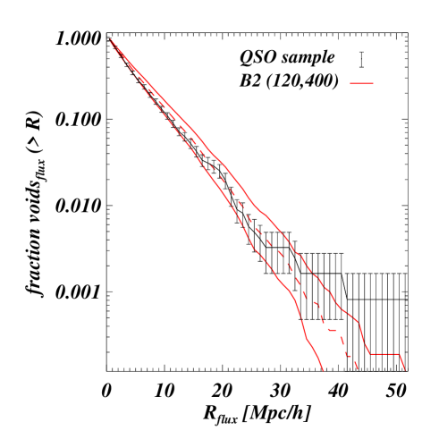
Figure 3: Fraction of 1D voids in the flux distribution at $z=2.2$ of size larger than $R$ as extracted from the observed sample ($1\sigma$ Poissonian error bars). Continuous lines represent the reference hydrodynamical simulation ($120$ Mpc$/h$) with voids identified taking $\pm 3\sigma$ values around the observed effective optical depth value (dashed line). The flux has been smoothed with a 1D top–hat filter of size $1$ Mpc$/h$.

We search for flux voids in the simulated spectra in the following simple way: $i)$ we extract 1000 lines–of–sight from the simulated volume; $ii)$ we normalize the mock spectra to have the observed mean flux value; $iii)$ we smooth the flux with a top–hat filter of size $1\,h^{-1}$ Mpc, which roughly corresponds to the comoving Jeans length; $iv)$ we identify connected flux regions above the mean flux level at the redshift of interest. The normalization is performed by multiplying the whole array of 1000 simulated optical depths arrays by a given constant (found iteratively after having extracted the spectra) in order to reproduce the wanted $\tau_{\rm eff}$ value. The choice of a different mean flux will of course impact on the void selection criterion, since a smaller (larger) mean flux level will increase (decrease) the number of pixels at high (low) transmissivity that are likely to correspond, in a non–trivial way, to under(over)-dense regions.

As a first preliminary test we check for the effects of resolution on the flux fractions of voids at $z=2$. Results are shown in Fig. 2, which shows simulations with different box sizes and resolutions, but with the same initial conditions normalized to the same mean flux. Note that this analysis is performed in redshift space and peculiar velocities affect the flux properties. From the Figure, it is clear that in order to sample the fraction of voids accurately a large enough volume and relatively high resolution are needed. For example, the $(120,200)$ simulation differs dramatically from the $(120,400)$ one, because in the latter relatively dense regions placed at the edge of void regions are better resolved. However, this discrepancy disappears once the flux is smoothed over a given scale (the Jeans length in our case). In a way, smoothing the flux degrades the resolution of the simulation making it less sensitive to the relevant physical processes causing absorption at and below the Jeans scale. Also note how increasing resolution beyond that in the $(120,400)$ simulation – the $(120,512)$ case – produce results that are well within the statistical error bars that are observed and will be shown in Figure 3. Because of this, $(120,400)$ is now taken to represent our fiducial run that will be used to explore other physically meaningful parameters.

We now perform the same search for the observed QSO spectra. The results are shown in Figure 3, which shows the distribution of the flux void population extracted from the observations (points with Poissonian error bars) and from our largest volume simulation. From the Figure it is clear that the fiducial $(120,400)$ run is in excellent agreement with observations and that flux voids of sizes $>35\,h^{-1}$ Mpc are about 1000 times less common than voids of sizes larger than few $h^{-1}$ Mpc. We also note a bump at around $20$ Mpc/$h$ in the voids fraction, but one would need a larger sample of QSOs in order to better test its statistical significance. The continuous lines show how the void fraction changes when the effective optical depth is varied at a $\pm 3\sigma$ level around the observed value. In particular, the lower and higher $\tau_{\rm eff}$ values ($\tau_{\rm eff}=0.136$ and $\tau_{\rm eff}=0.19$, respectively) have been chosen in such a way to conservatively embrace at a confidence level of $3\sigma$ the values obtained in Viel et al. (2004), where the measured value for the effective optical depth was $\tau_{\rm eff}=0.163\pm 0.009$. The recently determined power-law fit of Kim et al. (2007) $\tau_{\rm eff}=(0.0023\pm 0.0007)(1+z)^{3.65\pm 0.21}$ by using QSO spectra in the range $1.7<z<4$, is influenced by the scatter coming from QSO spectra over a large range of redshift, and would in principle allow for a larger range of effective optical depths. However, by selecting only a subsample at a given redshift, smaller statistical errors on the effective optical depth can be obtained.

We stress that the definition of void used here is based on the transmitted flux and thus is very different from studies based on the distribution of voids as inferred from the galaxy distribution.

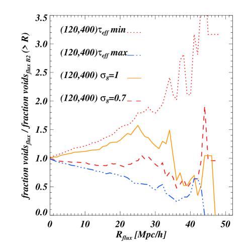
Figure 4: Ratio of the flux void fraction of the $(120,400)$ simulation ($\sigma_{8}=0.85$) with runs that use a different value of the power–spectrum amplitude ($\sigma_{8}=0.7$ and $\sigma_{8}=1$, represented by the dashed and continuous lines, respectively). Also shown are the ratios when the effective optical depth (which is used as a threshold to define voids in the flux distribution) of the reference run is conservatively varied between the observational bounds ($\pm 3\sigma$ values represented by the dot–dashed and dotted lines). Spectra have been normalized to the same effective optical depth.

4.2 Exploring the parameter space

We now discuss the main cosmological and astrophysical parameters that can affect the population of voids in the flux distribution. In Figure 4, we plot the ratios of the flux void fractions in the fiducial and in other simulations, where we changed $\tau_{\rm eff}$ at $z=2.2$ within the observational bounds and the value of $\sigma_{8}$. As could be expected, the fraction of voids changes dramatically with a change in $\tau_{\rm eff}$: at $z\sim 2$ the flux probability distribution function (pdf) is a steep function around the mean flux level. Thus adopting a different void selection criterion has a large impact on the void distribution. In the following, we normalize the mock QSO sample to reproduce the same effective optical depth. Changing $\sigma_{8}$ appears to have a smaller effect. A simulation with $\sigma_{8}=1$ results in a faster evolution of cosmic structures and in a 50$\%$ increase of the void population of size $R=20-35\,h^{-1}$ Mpc, compared with the reference $\sigma_{8}=0.85$ case. In the simulation with a lower value of $\sigma_{8}$, the void sizes are more evenly distributed. Note, however, that the trend at the largest sizes (45 Mpc$/h$) is somewhat different: here the low $\sigma_{8}$ simulation predicts more voids than the higher $\sigma_{8}$, since the smaller amount of power in the former can occasionally produce large regions devoid of matter and absorption. We also checked the impact of varying other parameters such as $\Omega_{m}$, $H_{0}$ and a change in the shape of the linear dark matter power spectrum in the initial conditions to account for a presence of warm dark matter (WDM) and adding some extra power (EP) at intermediate (from Mpc to tens of Mpc) scales, that results in an effect opposite to that of WDM. The mass chosen for the WDM particle is 0.15 keV. A mass that is already ruled out from the flux power spectrum of the Lyman-$\alpha$ forest (see Viel et al. (2007)) and that produces a suppression of power at scales around 0.4 Mpc$/h$, which are marginally sampled in the initial conditions of our (120,400) simulation. However, for the qualitative purposes of this paper this simulation should show the impact of a WDM particle on the distribution of the largest voids in the flux. At the scale of 2.5 Mpc$/h$ the power is 100 times higher (smaller) in the EP (WDM) simulation than the corresponding (120,400). The results are plotted in Figure 5, where all the simulations have the same value of $\sigma_{8}=0.85$: it is clear that the WDM and EP runs have opposite effects. WDM significantly enhance by a factor larger than 3 the fraction of largest voids, by erasing substructures below a given scale, while the EP simulation presents more collapsed structures that suppress the number of the largest voids. The effect of a larger value of $\Omega_{m}=0.4$ is similar to that of the EP simulation and determines a 90% reduction in the fraction voids whose sizes are larger than 30 Mpc$/h$. Finally, we checked for the effect of a smaller value of $H_{0}=45$ km/s/Mpc a value proposed recently by Alexander et al. (2007) to be the true value of the Hubble constant outside a local underdense region of very similar density to those explored here. Having a smaller value for the Hubble constant produces effects that are very similar to those of a smaller value of $\sigma_{8}=0.7$ (see Fig. 4): the evolution of the cosmic web is less pronounced and can occasionally produce large regions devoid of absorption, even if on average the effects are quite mild. We also varied the spectral index $n_{s}$ but found small differences to the reference case. As can be appreciated from Figure 3, the statistical errors on the observed void fraction are somewhat large and thereby distinguishing between different cosmological model is still very difficult and none of the models presented here could be convincingly ruled out.

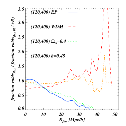
Figure 5: Ratio of the flux void fraction of the $(120,400)$ simulation ($\sigma_{8}=0.85$) with runs that have some extra power (EP, continuous line) and less power (WDM, dashed line) at Mpc scales. Also shown are the ratios when the Hubble constant is set to a smaller $h=0.45$ value (dot-dashed line) and a simulation with a larger value of $\Omega_{m}=0.4$ (dotted line). The reference B2 (120,400) run has $h=0.72$ and $\Omega_{m}=0.26$. Spectra have been normalized to the same effective optical depth.

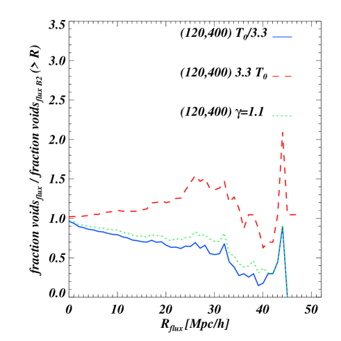
Figure 6: Ratio of the flux void fraction for the $(120,400)$ runs, comparing the fiducial run ($\gamma=1.6$ and $T=T_{0}$) with runs that have a different value of the IGM temperature at mean density ($2\,T_{0}$ and $T_{0}$ are represented by dashed and continuous lines, respectively) and with a run that has a different value of $\gamma$ (dotted line). Spectra have been normalized to the same effective optical depth.

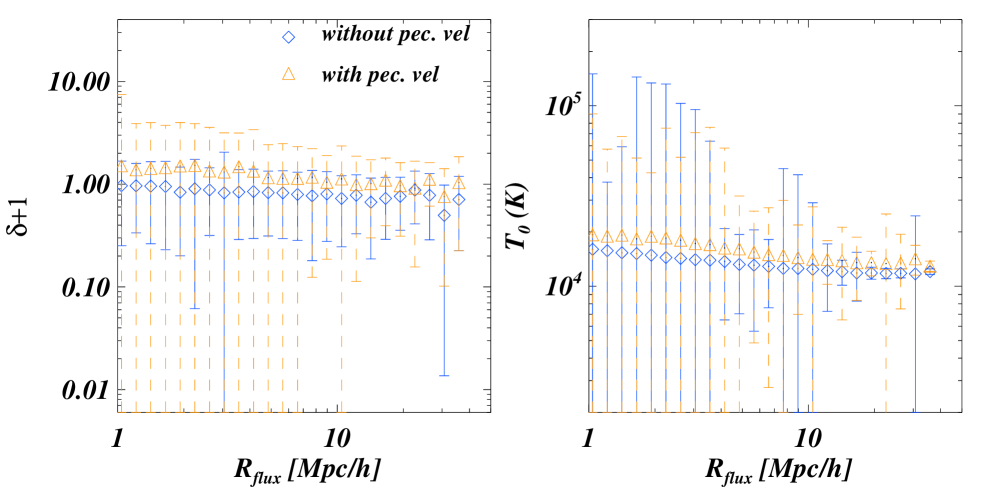
Figure 7: 1D gas density and temperature in void regions along lines–of–sight extracted from the fiducial simulation at $z=2.2$. Voids have been identified from the flux distribution as regions above the mean flux level. Results are shown with (triangles) and without (diamonds) peculiar velocities, and error bars represent the scatter.

Several other parameters could have an impact on the void distribution, in particular the two parameters that are poorly constrained and that describe the thermal state of the IGM: $T_{0}$ and $\gamma$. We investigate the effect of a different value of $T_{0}$ in Figure 6. A colder (hotter) IGM will result in a higher (lower) density of neutral hydrogen and thereby in more absorptions, which, in turn, will decrease (increase) the fraction of large voids. In Figure 6, we also overplot the effect of changing $\gamma$ from the reference value ($\gamma=1.6$) to $\gamma=1.1$ (represented by the dotted line in the Figure), which is a better fit to the data at this redshift (Bolton et al., 2007). A flatter equation of state will not only make underdense regions hotter, but it will also make the slightly overdense regions colder. The overall effect is a slight decrease in the fraction of flux voids, since cold regions embed on average more neutral hydrogen than hot ones. This result shows that by selecting mean–flux–level regions we are sampling regions around mean density (for which the power–law ’equation of state’ could be a poor fit to the actual distribution).

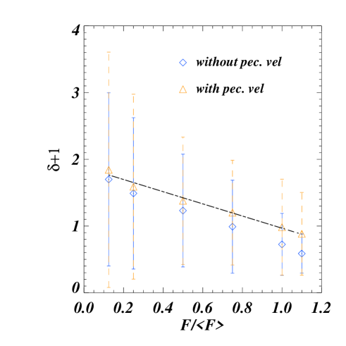
Figure 8: Densities of voids (larger than 7$\,h^{-1}$ Mpc) as a function of flux threshold level at $z=2.2$. Results are shown with (triangles) and without (diamonds) peculiar velocities, and error bars represent the scatter. The dashed line shows a linear fit to the case with peculiar velocities.

Note that the effect of changing $\gamma$ was addressed by running a new simulation that self–consistently results in a low $\gamma$ at $z=2$ (using a modified version of the GADGET-2 code kindly provided by J. Bolton) and not by rescaling the gas-temperature relation a posteriori as is sometimes done. Another important input parameter is the overall amplitude of the UVB, parametrized by $\Gamma_{-12}$, for which we have some observational constraints (Bolton et al., 2005). However, this quantity is degenerate with the value of $\tau_{\rm eff}$, so changing $\Gamma_{-12}$ will result in the same change as changing $\tau_{\rm eff}$.

4.3 From flux to 1D gas density

Having identified voids at $z\sim 2$, using the mean flux as a threshold, we are now interested in linking the flux properties to the underlying physical properties of the gas density field. The main problem we have to deal with is that the flux is observed in redshift space, while we want to recover gas properties in real space. The role of peculiar velocities in determining the properties of the transmitted flux has been investigated by several authors (e.g. Weinberg et al. (1998)), however for the purpose of the analysis performed here it produces a shift of the absorption feature from the real space overdensity to the redshift space observed flux. This increases the scatter since redshift space pixels are not related in a simple manner to the underlying real space density field.

Occasionally, peculiar velocities could be of the order of a few hundred km/s, so the correspondence is non-trivial (see for example Rauch et al. (2005)). However, we can rely on hydrodynamical simulations in order to infer, at least on a statistical basis, the physical properties of the gas. In Figure 7, we show the mean values and scatter (r.m.s. values) in the real space gas–overdensity and temperature fields, corresponding to the flux voids of the previous sections. We show the fields both without (diamond symbols) and with (triangles) peculiar velocities, which alter the flux distribution observed in velocity space. From the plot, it is clear that selecting regions above mean flux at $z\sim 2$, as we did in the previous Sections, allows us to identify and measure (with a large error bar) the density in 1D gas voids with sizes larger than $\sim 10\,h^{-1}$ Mpc in the case with peculiar velocities. If peculiar velocities are neglected the scatter is much smaller (as expected), and the density can be measured for somewhat smaller voids (sizes larger than $\sim 7\,h^{-1}$ Mpc). For even smaller voids only upper limits of the order a few times mean density can be set, and very little can be inferred about their temperature. The gas temperature inside the largest flux voids is of the order of $10^{4}$ K. These regions are thus cold and, as expected from the nature of Lyman-$\alpha$ forest absorptions, sample the IGM ‘equation of state’ around mean density. Therefore, even when peculiar velocities are taken into account, the physical properties of the largest voids can be reliably studied. Furthermore, note that the effect of the peculiar velocities for the recovered mean density and temperature inside voids is systematically slightly higher than the corresponding values for the case when peculiar velocities are neglected. As before, this effect is expected since the peculiar velocity shift can move some denser clumps of gas into voids regions that increase their overall mean density. We stress that the ’gas voids’ defined in this Section, as identified from the transmitted flux, do not correspond to underdense regions in the gas distribution but to regions around the mean density.

In Fig. 8 we plot the voids’ densities for voids whose sizes are larger than 7$\,h^{-1}$ Mpc, with and without peculiar velocities and with a varying flux threshold. The scatter is large, but for voids regions above the mean flux level in 68$\%$ of all cases these regions have overdensities in the range $\delta=[-0.8,0.8]$. If the flux threshold is lowered, large voids regions start to sample environments at higher overdensities. The dashed line represents a linear fit to the points (with peculiar velocities): $\delta+1\equiv\rho/<\rho>=-0.9\,F/<F>+1.9$. This relation should describe the mean 1D density of large ($>7$ comoving Mpc$/h$) voids identified in the flux distribution at $z\sim 2$, as derived from high-resolution Lyman-$\alpha$ forest QSOs spectra. We note that a systematic trend is present and the recovered gas density is larger in the case with peculiar velocities: we attribute this to the fact that with peculiar velocities the corresponding gas absorptions are shifted and a void region identified in the flux is not simply related to an underdense region but can incorporate regions at higher density that will increase the recovered global density.

4.4 From 1D gas density to the 3D dark matter distribution

In this Section, we link the 1D properties of flux voids to the 3D dark matter properties. We use a void–finding algorithm for the dark matter distribution of the reference simulation. The algorithm is described in more detail in Colberg et al. (2005). Its main features can be summarized as follows. The starting point for the void finder is the adaptively smoothed distribution of the matter distribution in the simulation. Proto–voids are constructed as spheres whose average overdensity is below a threshold value $\delta_{t}$, which is a free parameter. These proto–voids are centered on local minima in the density field. Proto–voids are then merged according to a set of criteria, which allow for the construction of voids that can have any shape, as long as two large regions are not connected by a thin tunnel (which would make the final void look like a dumbell). The voids thus can have arbitrary shapes, but they typically look like lumpy potatoes. For each void, we compute the radius $R_{DM}$ of a sphere whose volume equals that of the void. While strictly speaking $R_{DM}$ is not the actual radius of the void, it provides a useful measure of the size of the void. In this work here, we adopt a value of $\delta_{t}=-0.5$ (for a justification of this choice see below). As a first, preliminary check, we compared the void size distribution of the fiducial simulation with earlier results by Colberg et al. (2005) and found good agreement. Note that the size of the grid used for the density field limits the sizes of the smallest voids that can be found with this void finder – in our case 1$\,h^{-1}$ Mpc. However, as discussed above, peculiar velocities make studies of voids smaller than 7$\,h^{-1}$ Mpc very hard, so we need not be concerned about the smallest voids at all.

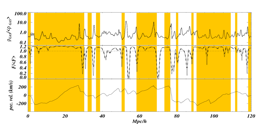
Figure 9: Relation between 3D dark matter voids and physical quantities along the line–of–sight to distant QSOs. The intersections of 3D real–space voids in the dark matter distribution along the line–of–sight are represented by shaded rectangles. The top panel shows the 1D real–space gas overdensity, the middle one the simulated Lyman-$\alpha$ flux in redshift space, the bottom panel the peculiar velocity field in km/s. Absorption features in the flux distribution correspond to overdensity peaks shifted by the peculiar velocity of the bottom panel (100 km/s roughly corresponds to 1 $h^{-1}$ Mpc comoving). The dotted line in the flux distribution sets the criterion for the void definition, while the dashed one represents the flux smoothed over 1 $h^{-1}$ Mpc. This particular line–of–sight is taken along the x-axis and at a y-coordinate of 93 Mpc$/h$ in the slice of Figure 1.

As a qualitative example, in Figure 9 we show one line–of–sight through the simulated volume. We plot the 1D gas density field in real space (top panel), the simulated flux (middle panel) in redshift space, and the gas peculiar velocity field in km/s (bottom panel) in real space. The $x$–axis indicates the comoving (real space) coordinate along the line–of–sight. Flux absorption is usually produced by gas overdensities shifted by the peculiar velocity associated to the same gas element. For example, the absorption in the flux at 70 Mpc/$h$ is produced by the gas density peak at around 68 Mpc$/h$, shifted by $\sim 200$ km/s – which corresponds to roughly 2 $h^{-1}$ Mpc.

The shaded regions show the intersections with the line–of–sight of 3D voids in the dark matter distribution identified with the void finder algorithm described above. In the middle panel we overplot the mean flux level as a dotted line, with the flux smoothed on a scale of 1 $h^{-1}$ Mpc, as in Section 4.1. We find that the choice of threshold overdensity $\delta_{t}=-0.5$ for the 3D void finder results in a good correspondence of the resulting voids with voids defined in the flux distribution. From the bottom panel of Figure 9 it is clear that the void regions are expanding, and the gas velocity fields for the largest voids are of the order of $\pm$ 200 km/s (see the void centered on around 20 Mpc$/h$). These high redshift voids in the IGM will keep growing, get emptier of matter and could be the progenitors of lower redshifts voids of sizes similar to the Tully void (Tully (2007)). The peculiar velocities along the line–of–sight rise smoothly from negative values to positive ones and are sandwiched by regions in which the peculiar velocity shows a negative gradient, which could be the signature of a moderate shock. It is worth emphasizing that these velocity profiles are not always completely symmetric because the line–of–sight does not necessarily pierce the 3D voids in their centers. Moreover, from the top panel it is clear that the 1D density profile inside the void is quite complex, showing small density peaks, which correspond to small haloes that most likely host the observed void galaxy population.

In order to provide a more quantitative picture, in Figure 10 we plot the underlying mean values of 1D quantities obtained once the 3D voids have been identified (using $\delta_{t}=-0.5$). The top panel represents the probability distribution function of the sizes of such 1D flux voids, while in the other three panels each point shows, from top to bottom, the mean gas overdensity, flux and peculiar velocity field for a given 3D DM void. Note that while in Section 4.1 we were interested in measuring the properties of voids once the mean flux threshold was set as a criterion to define voids, here we use the 3D DM distribution to look for the corresponding 1D (Lyman-$\alpha$ forest) flux–related quantities.

The overall picture suggests that large voids ($>7-10$ Mpc$/h$) are usually related to flux values above the mean, and the corresponding mean values of gas density and peculiar velocities have less scatter than smaller voids. The corresponding mean value for the gas overdensity is $\delta_{\mbox{GAS}}=-0.43$, so the 3D void region is slightly denser in gas than in dark matter, something that can be expected since baryons feel pressure and are thus more diffused than the collisionless dark matter (e.g. Viel et al. (2002)). The different value of $\delta_{\mbox{GAS}}$ than the one found in Section 4.3 does not contradict our earlier findings, since now the requirement to define a void is less stringent. Now, the actual void has to be a quasi–spherical 3D region in the DM distribution and not a connected 1D region with flux above the mean flux. This means that in 1D one is more sensitive to clumps of matter producing absorptions, while the same clump will have a smaller impact on the mean density of the 3D region surrounding it. Cases for which the flux voids correspond to actual DM voids are avaraged out statistically by small lumps of gas around the mean density along the line–of–sight, that cause absorption and do not alter the global 3D DM density of the void region

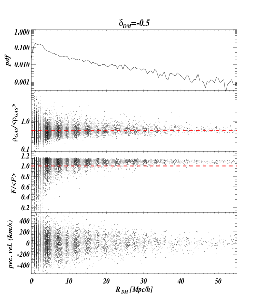
Figure 10: Voids in the 3D dark matter distribution have been identified with the algorithm described in the text using a density threshold of $\delta_{DM}=-0.5$. Here we plot the 1D void flux pdf, the 1D gas median overdensity along the line–of–sight for each identified void in the 3D dark matter distribution, the median $F/<F>$ value in the void and the median peculiar velocity for the same void region (from top to bottom).

For this population of large voids the typical scatter in the peculiar velocity field is 170 km/s. We thus have shown that the population of 1D large flux voids, i.e. regions above the mean flux level, as estimated from a set of mock high resolution spectra at $z\sim 2$, traces reasonably faithfully a population of 3D dark matter voids of similar sizes, with a typical $\delta_{t}=-0.5$.

We have also checked that the scatter plots of Figure 10 are not very sensitive to the cosmological model (i.e. different values of $\sigma_{8}$), which means that the voids physical properties are the same for different values of the power spectrum amplitude.

5 Conclusions and perspectives

We used Lyman-$\alpha$ forest QSO spectra to constrain the void population at $z\sim 2$ at a range of scales and redshifts, which cannot be probed by other observables. The main conclusions can be summarized as follows:

• the properties (sizes) of voids identified in simulations from the flux distribution as connected regions above the mean flux level are in good agreement with observed ones;

• using a set of hydrodynamical simulations and varying all the astrophysical and cosmological parameters, along with checking box size and resolution effects, we find that the flux void size distribution is a robust statistics that depends primarily on the flux threshold chosen to define the voids;

• the flux seems to be a reliable tracer of the underlying dark matter distribution, altering the statistical properties of the dark matter density field (changing amplitude, shape, adding or suppressing power in a wavenumber dependent manner) changes the properties of the void population although at present is difficult to give constraints on cosmological parameters using these statistics;

• flux voids, i.e. connected regions above the mean flux levels, correspond to gas densities around the mean density, regardless of the role of peculiar velocities, which contribute to a scatter in this relation, but do not alter significantly the mean values;

• linking 1D voids to the corresponding 3D dark matter voids is more difficult, and we used a void–finding algorithm for that: we find that 3D DM voids with a mean overdensity of $\delta_{t}=-0.5$ correspond to the flux voids that we have defined from the QSO spectra. However, the correspondence is good only for voids with sizes larger than about $7-10$ Mpc$/h$.

In this paper, we made a preliminary attempt to link the population of voids in the transmitted Lyman-$\alpha$ flux to the underlying 1D gas density and temperature and 3D dark matter density. The use of Lyman-$\alpha$ high–resolution spectra is important in the sense that it explores a new regime in scales, redshifts and densities which is currently not probed by other observables: the scales are of order few to tens of Mpc, the redshift range is between $z=2-4$, while the densities are around the mean density. Further studies, that could possibly rely on wider data sets such as the low–resolution SDSS data (Shang et al. (2007)), on other future observables at higher redshifts (D’Aloisio & Furlanetto (2007)) or on tomographic studies involving QSO pairs or multiple line–of–sights (D’Odorico et al. (2006), Saitta et al. (2007)) would be important in understanding the dynamical, thermal and chemical evolution of the void population and the interplay between galaxy and the IGM over a large fraction of the Hubble time.

References

- Alexander et al. (2007) Alexander S., Biswas T., Notari A., Vaid D., 2007, ArXiv e-prints, 712
- Arbabi-Bidgoli & Müller (2002) Arbabi-Bidgoli S., Müller V., 2002, MNRAS, 332, 205
- Benson et al. (2003) Benson A. J., Hoyle F., Torres F., Vogeley M. S., 2003, MNRAS, 340, 160
- Bi & Davidsen (1997) Bi H., Davidsen A. F., 1997, ApJ, 479, 523
- Bolejko et al. (2005) Bolejko K., Krasiński A., Hellaby C., 2005, MNRAS, 362, 213
- Bolton et al. (2006) Bolton J. S., Haehnelt M. G., Viel M., Carswell R. F., 2006, MNRAS, 366, 1378
- Bolton et al. (2005) Bolton J. S., Haehnelt M. G., Viel M., Springel V., 2005, MNRAS, 357, 1178
- Bolton et al. (2007) Bolton J. S., Viel M., Kim T. ., Haehnelt M. G., Carswell R. F., 2007, ArXiv e-prints, 711
- Brunino et al. (2007) Brunino R., Trujillo I., Pearce F. R., Thomas P. A., 2007, MNRAS, 375, 184
- Caldwell & Stebbins (2007) Caldwell R. R., Stebbins A., 2007, ArXiv e-prints, 711
- Ceccarelli et al. (2006) Ceccarelli L., Padilla N. D., Valotto C., Lambas D. G., 2006, MNRAS, 373, 1440
- Colberg et al. (2005) Colberg J. M., Sheth R. K., Diaferio A., Gao L., Yoshida N., 2005, MNRAS, 360, 216
- Crotts (1987) Crotts A. P. S., 1987, MNRAS, 228, 41P
- D’Aloisio & Furlanetto (2007) D’Aloisio A., Furlanetto S. R., 2007, ArXiv e-prints, 710
- Dobrzycki & Bechtold (1991) Dobrzycki A., Bechtold J., 1991, ApJ, 377, L69
- D’Odorico et al. (2006) D’Odorico V., Viel M., Saitta F., Cristiani S., Bianchi S., Boyle B., Lopez S., Maza J., Outram P., 2006, MNRAS, 372, 1333
- Duncan et al. (1989) Duncan R. C., Ostriker J. P., Bajtlik S., 1989, ApJ, 345, 39
- Faucher-Giguere et al. (2007) Faucher-Giguere C. ., Prochaska J. X., Lidz A., Hernquist L., Zaldarriaga M., 2007, ArXiv e-prints, 709
- Furlanetto & Piran (2006) Furlanetto S. R., Piran T., 2006, MNRAS, 366, 467
- Goldberg et al. (2005) Goldberg D. M., Jones T. D., Hoyle F., Rojas R. R., Vogeley M. S., Blanton M. R., 2005, ApJ, 621, 643
- Goldberg & Vogeley (2004) Goldberg D. M., Vogeley M. S., 2004, ApJ, 605, 1
- Gottlöber et al. (2003) Gottlöber S., Łokas E. L., Klypin A., Hoffman Y., 2003, MNRAS, 344, 715
- Gunn & Peterson (1965) Gunn J. E., Peterson B. A., 1965, ApJ, 142, 1633
- Haardt & Madau (1996) Haardt F., Madau P., 1996, ApJ, 461, 20
- Hoeft et al. (2006) Hoeft M., Yepes G., Gottlöber S., Springel V., 2006, MNRAS, 371, 401
- Hoyle et al. (2005) Hoyle F., Rojas R. R., Vogeley M. S., Brinkmann J., 2005, ApJ, 620, 618
- Hoyle & Vogeley (2004) Hoyle F., Vogeley M. S., 2004, ApJ, 607, 751
- Jena et al. (2005) Jena T., Norman M. L., Tytler D., Kirkman D., Suzuki N., Chapman A., Melis C., Paschos P., O’Shea B., So G., Lubin D., Lin W.-C., Reimers D., Janknecht E., Fechner C., 2005, MNRAS, 361, 70
- Kim et al. (2007) Kim T. ., Bolton J. S., Viel M., Haehnelt M. G., Carswell R. F., 2007, MNRAS, 382, 1657
- Kim et al. (2004) Kim T.-S., Viel M., Haehnelt M. G., Carswell R. F., Cristiani S., 2004, MNRAS, 347, 355
- Lee & Park (2006) Lee J., Park D., 2006, ApJ, 652, 1
- Lesgourgues et al. (2007) Lesgourgues J., Viel M., Haehnelt M. G., Massey R., 2007, Journal of Cosmology and Astro-Particle Physics, 11, 8
- Mathis & White (2002) Mathis H., White S. D. M., 2002, MNRAS, 337, 1193
- McDonald et al. (2000) McDonald P., Miralda-Escudé J., Rauch M., Sargent W. L. W., Barlow T. A., Cen R., Ostriker J. P., 2000, ApJ, 543, 1
- McLin et al. (2002) McLin K. M., Stocke J. T., Weymann R. J., Penton S. V., Shull J. M., 2002, ApJ, 574, L115
- Naselsky et al. (2007) Naselsky P. D., Christensen P. R., Coles P., Verkhodanov O., Novikov D., Kim J., 2007, ArXiv e-prints, 712
- Neyrinck (2007) Neyrinck M. C., 2007, ArXiv e-prints, 712
- Ostriker et al. (1988) Ostriker J. P., Bajtlik S., Duncan R. C., 1988, ApJ, 327, L35
- Padilla et al. (2005) Padilla N. D., Ceccarelli L., Lambas D. G., 2005, MNRAS, 363, 977
- Park & Lee (2007) Park D., Lee J., 2007, Physical Review Letters, 98, 081301
- Patiri et al. (2006c) Patiri S. G., Betancort-Rijo J., Prada F., 2006c, MNRAS, 368, 1132
- Patiri et al. (2006a) Patiri S. G., Betancort-Rijo J. E., Prada F., Klypin A., Gottlöber S., 2006a, MNRAS, 369, 335
- Patiri et al. (2006b) Patiri S. G., Prada F., Holtzman J., Klypin A., Betancort-Rijo J., 2006b, MNRAS, 372, 1710
- Peebles (2001) Peebles P. J. E., 2001, ApJ, 557, 495
- Peebles (2007) Peebles P. J. E., 2007, ArXiv e-prints, 712
- Rauch et al. (2005) Rauch M., Becker G. D., Viel M., Sargent W. L. W., Smette A., Simcoe R. A., Barlow T. A., Haehnelt M. G., 2005, ApJ, 632, 58
- Rauch et al. (1992) Rauch M., Carswell R. F., Chaffee F. H., Foltz C. B., Webb J. K., Weymann R. J., Bechtold J., Green R. F., 1992, ApJ, 390, 387
- Rojas et al. (2004) Rojas R. R., Vogeley M. S., Hoyle F., Brinkmann J., 2004, ApJ, 617, 50
- Rojas et al. (2005) Rojas R. R., Vogeley M. S., Hoyle F., Brinkmann J., 2005, ApJ, 624, 571
- Rudnick et al. (2007) Rudnick L., Brown S., Williams L. R., 2007, ArXiv e-prints, 704
- Saitta et al. (2007) Saitta F., D’Odorico V., Bruscoli M., Cristiani S., Monaco P., Viel M., 2007, ArXiv e-prints, 712
- Schaye (2001) Schaye J., 2001, ApJ, 559, 507
- Shandarin et al. (2006) Shandarin S., Feldman H. A., Heitmann K., Habib S., 2006, MNRAS, 367, 1629
- Shang et al. (2007) Shang C., Crotts A., Haiman Z., 2007, ArXiv e-prints, 705
- Sheth & van de Weygaert (2004) Sheth R. K., van de Weygaert R., 2004, MNRAS, 350, 517
- Springel (2005) Springel V., 2005, MNRAS, 364, 1105
- Stocke et al. (1995) Stocke J. T., Shull J. M., Penton S., Donahue M., Carilli C., 1995, ApJ, 451, 24
- Tikhonov & Karachentsev (2006) Tikhonov A. V., Karachentsev I. D., 2006, ApJ, 653, 969
- Tully (2007) Tully R. B., 2007, ArXiv e-prints, 708
- van de Weygaert & Schaap (2007) van de Weygaert R., Schaap W., 2007, ArXiv e-prints, 708
- Viel et al. (2007) Viel M., Becker G. D., Bolton J. S., Haehnelt M. G., Rauch M., Sargent W. L. W., 2007, ArXiv e-prints, 709
- Viel et al. (2006) Viel M., Haehnelt M. G., Lewis A., 2006, MNRAS, 370, L51
- Viel et al. (2004) Viel M., Haehnelt M. G., Springel V., 2004, MNRAS, 354, 684
- Viel et al. (2004b) Viel M., Matarrese S., Heavens A., Haehnelt M. G., Kim T.-S., Springel V., Hernquist L., 2004b, MNRAS, 347, L26
- Viel et al. (2002) Viel M., Matarrese S., Mo H. J., Theuns T., Haehnelt M. G., 2002, MNRAS, 336, 685
- Weinberg et al. (1998) Weinberg D. H., Hernsquit L., Katz N., Croft R., Miralda-Escudé J., 1998, in Petitjean P., Charlot S., eds, Structure et Evolution du Milieu Inter-Galactique Revele par Raies D’Absorption dans le Spectre des Quasars, 13th Colloque d’Astrophysique de l’Institut d’Astrophysique de Paris Hubble Flow Broadening of the Ly Forest and its Implications. pp 133–+