A Precise Proper Motion for the Crab Pulsar, and the Difficulty of Testing Spin-Kick Alignment for Young Neutron Stars

D. L. Kaplan¹¹affiliation: Pappalardo Fellow and Hubble Fellow; Kavli Institute for Astrophysics and Space Research and Department of Physics, Massachusetts Institute of Technology, Cambridge, MA 02139; dlk@space.mit.edu. , S. Chatterjee²²affiliation: School of Physics, The University of Sydney, NSW 2006, Australia; schatterjee, bgaensler@usyd.edu.au , B. M. Gaensler²²affiliation: School of Physics, The University of Sydney, NSW 2006, Australia; schatterjee, bgaensler@usyd.edu.au ³³affiliation: Harvard-Smithsonian Center for Astrophysics, Cambridge, MA 02138 , and J. Anderson⁴⁴affiliation: Department of Physics and Astronomy, Rice University, Houston, TX 77251; jay@eeyore.rice.edu

Abstract

We present a detailed analysis of archival Hubble Space Telescope data that we use to measure the proper motion of the Crab pulsar, with the primary goal of comparing the direction of its proper motion with the projected axis of its pulsar wind nebula (the projected spin axis of the pulsar). Combining data from 47 observations spanning $>10\,$ yr with two different instruments, and using the best available measurement techniques and latest distortion models, we are able to demonstrate that our measurement is robust and has an uncertainty of only $\pm 0.4\,\mbox{mas}\,\mbox{yr}^{-1}$ on each component of the proper motion. However, we then consider the various uncertainties that arise from the need to correct the proper motion that we measure to the local standard of rest at the position of the pulsar and find $\mu_{\alpha}=-11.8\pm 0.4\pm 0.5\,\mbox{mas}\,\mbox{yr}^{-1}$ and $\mu_{\delta}=\mbox{+4.4}\pm 0.4\pm 0.5\,\mbox{mas}\,\mbox{yr}^{-1}$ relative to the pulsar’s standard of rest, where the two uncertainties are from the measurement and the reference frame, respectively. If we then wish to compare this proper motion to the symmetry axis of the pulsar wind nebula, we must consider the unknown velocity of the pulsar’s progenitor (assumed to be $\sim 10\,\mbox{km}\,\mbox{s}^{-1}$ ), and hence add an additional uncertainty of $\pm 2\,\mbox{mas}\,\mbox{yr}^{-1}$ to each component of the proper motion, although this could be a factor of 10 larger if the pulsar’s progenitor had an anomalously high velocity ( $>100\,\mbox{km}\,\mbox{s}^{-1}$ ). This implies a projected misalignment with the nebular axis of $14\arcdeg\pm 2\arcdeg\pm 9\arcdeg$ , consistent with a broad range of values including perfect alignment. We use our proper motion to derive an independent estimate for the site of the supernova explosion with an accuracy that is 2–3 times better than previous estimates. We conclude that the precision of individual measurements which compare the direction of motion of a neutron star to a fixed axis will often be limited by fundamental uncertainties regarding reference frames and progenitor properties. The question of spin-kick (mis)alignment, and its implications for asymmetries and other processes during supernova core-collapse, is best approached by considering a statistical ensemble of such measurements, rather than detailed studies of individual sources.

Subject headings:

astrometry — pulsars: individual (PSR B0531+21, Crab) — stars: neutron

^†^†slugcomment: Accepted for Publication in ApJ

1. Introduction

The high velocity nature of the neutron star population has been apparent almost as long as the existence of neutron stars has been recognized (Gunn & Ostriker, 1970). Recent statistical studies of the radio pulsar velocity distribution (e.g., Arzoumanian et al., 2002; Brisken et al., 2003; Hobbs et al., 2005; Faucher-Giguère & Kaspi, 2006) yield mean three-dimensional velocities of 300–500 $\mbox{km}\,\mbox{s}^{-1}$ , with a high velocity tail extending beyond 1000 $\mbox{km}\,\mbox{s}^{-1}$ .

A variety of physical mechanisms have been proposed as the origin of high velocities. Perhaps the first was disruption of binaries through mass loss in supernovae (Blaauw 1961; Gott, Gunn, & Ostriker 1970; Iben & Tutukov 1996), although it is difficult for binary disruption alone to account for some of the highest observed velocities (Harrison, Lyne, & Anderson 1993; Chatterjee et al. 2005). The most natural source of such high velocities appears to be asymmetries in the birth supernovae of pulsars (Shklovskii, 1970; van den Heuvel & van Paradijs, 1997; Portegies Zwart & van den Heuvel, 1999), although exactly how an asymmetry in the core collapse process in a supernova explosion is converted to a birth kick imparted to a nascent neutron star remains unclear (Lai, Chernoff, & Cordes, 2001). While hydrodynamic or convective instabilities are the most plausible route (e.g., Burrows & Hayes, 1996; Janka & Mueller, 1996; Lai & Goldreich, 2000; Scheck et al., 2004; Janka et al., 2005; Scheck et al., 2006; Burrows et al., 2006), more exotic mechanisms such as asymmetric neutrino emission in the presence of strong magnetic fields (Arras & Lai, 1999) or some combination of the above (Socrates et al., 2005) cannot be ruled out.

Of these kick mechanisms, many predict kicks vectors that relate to the spin axis orientation of the nascent neutron star: the alignment (or lack thereof) of the natal kick with the neutron star spin axis could provide a specific discriminant between various mechanisms (Burrows, Hayes, & Fryxell 1995; Spruit & Phinney 1998; Cowsik 1998; Lai et al. 2001; Romani 2005). Even such parameters such as the number and timescale of kick components, coupled with the initial spin period of the neutron star, can be constrained through observations of an ensemble of sources (Deshpande, Ramachandran, & Radhakrishnan 1999; Johnston et al. 2006; Wang et al. 2006, 2007; Ng & Romani 2007; Rankin 2007).

1.1. The Crab Pulsar and its Nebula

The Crab pulsar (PSR B0531+21 (catalog PSR B0531+21)) and nebula have been observed by virtually every telescope capable of pointing at the system, and the Crab may be the most studied system in all of astronomy. The Crab nebula possesses a general symmetry axis, visible in images at most wavelengths. Recent observations have delineated this axis with striking clarity (e.g., Hester et al., 2002; Ng & Romani, 2004). The X-ray jet, in particular, allows us to trace the symmetry axis to the neutron star location, and provides a natural association with the rotation axis of the pulsar itself (since every other vector would be rotation averaged). The symmetry axis is roughly aligned with the proper motion (e.g., Caraveo & Mignani, 1999), but the observational uncertainties have made the alignment hard to quantify. A precise proper motion vector for the Crab pulsar could be quantitatively compared to the jet direction to establish whether the natal kick is aligned with the spin axis, as many theories predict.

Given its prominent place in our understanding of neutron stars, it is perhaps surprising that the proper motion and distance of the Crab pulsar are not better known. Compared to many fainter objects, the precision of our measurements is lacking. While there were a number of early attempts to measure the proper motion of the Crab pulsar, these were generally inconsistent with each other (Minkowski, 1970). Perhaps the first reliable measurement was that of Wyckoff & Murray (1977, hereafter WM77), who found¹¹1The analysis of WM77 was based on the B1950 frame, but at this level of precision the precession between that and the J2000 frame does not change the proper motion significantly. $(\mu_{\alpha},\mu_{\delta})=(-13\pm 2,7\pm 3)\,\mbox{mas}\,\mbox{yr}^{-1}$ from photographic plates spanning epochs from 1899 to 1976. There have not been any direct (i.e. geometric) distance measurements of the pulsar itself, but the distance was estimated based on various lines of evidence to lie between 1.4 and 2.7 kpc (Trimble, 1973). In spite of the wealth of observations since then, including a treasure trove of Hubble Space Telescope (HST) images with a time baseline of $>10$ years, these estimates had not significantly improved until recently. For example, Caraveo & Mignani (1999, hereafter CM99) estimate a proper motion $(\mu_{\alpha},\mu_{\delta})=(-17\pm 3,7\pm 3)\,\mbox{mas}\,\mbox{yr}^{-1}$ , which is consistent with the earlier estimate, but does not improve upon its accuracy.

The main obstacle to more accurate measurements is not (as in many cases) the limitations of faint objects, but rather the fact that the Crab nebula is too bright for most interferometric radio observations (it raises the system temperature too much), that there are no suitable interferometric calibrators nearby, and that the rotational stability is not sufficient (due to glitches) for precise pulse timing over a long time baseline. Because of these reasons, high angular resolution optical observations are so far the only way to measure the astrometric parameters (proper motion and parallax) of the Crab pulsar, and with the current generation of instruments we are limited to data from HST.

Ng & Romani (2006, hereafter NR06) attempted a significantly more detailed astrometric analysis of the Crab pulsar compared to CM99, taking advantage of new HST data spanning 7 years and trying to account for many sources of uncertainty not addressed by CM99. NR06 found a result that is discrepant with that of CM99: $(\mu_{\alpha},\mu_{\delta})=(-15.0\pm 0.8,1.3\pm 0.8)\,\mbox{mas}\,\mbox{yr}^{-1}$ . This shows a significant misalignment with the projected spin-axis of the pulsar ( $26\arcdeg\pm 3\arcdeg$ ) and as such reverses previously held notions of spin-kick alignment, but as we discuss below (and as NR06 acknowledge) even this analysis still is not as accurate as possible. Additionally, a large number of new observations with the Advanced Camera for Surveys (ACS) have become publicly available. These were taken primarily for studying the dynamics and polarization of the Crab’s pulsar wind nebula (e.g., Hester et al., 2002), and as such they were not ideal for astrometry (the exposure times were long enough that the pulsar saturated, the dithering strategy was not optimal, and they used a limited range of roll angle), but nonetheless they are an important resource.

Motivated by the importance of the Crab pulsar in our understanding of neutron stars and supernova remnants in general, by the large amount of data available on it, and by the limitations of previous analyses, we have attempted to re-measure the proper motion of the Crab pulsar as well as assess the possibility of a parallax measurement with future data (although given the recent failure of the ACS instrument, future observations may not be possible until the installation of the upcoming Wide Field Camera 3).

The organization of our paper is as follows: in § 2 we describe our analysis, noting departures from previous analyses, although the majority of the fitting techniques are similar to those we used in Kaplan, van Kerkwijk, & Anderson (2007), and we refer readers there for more details. After refining the proper motion measurement, we discuss in § 2.5 the limitations on our knowledge of the proper motion imposed by the unknown velocity of the pulsar’s progenitor, as well as uncertainties in the corrections to the pulsar’s local standard of rest. These transformations and their associated uncertainties limit the accuracy of the comparison between the proper motion and the projected spin-axis of the pulsar. We then give our conclusions in § 3. Finally, we include a discussion of the prospects for a parallax distance for the Crab pulsar in Appendix A. In what follows, we define our proper motions in Right Ascension and Declination $(\mu_{\alpha},\mu_{\delta})$ so that the scales are the same and no $\cos\delta$ term is necessary. All uncertainties are 1- $\sigma$ unless otherwise stated, and all position angles are measured east of north.

2. Analysis

We started our analysis by examining the available archival HST data for the Crab pulsar. Twenty observations using the Wide Field and Planetary Camera 2 (WFPC2) with the F547M filter (a filter centered at $V$ -band but somewhat narrower, designed to avoid bright emission lines) spanning $\sim$ 2 years were analyzed by CM99, who were able to determine a proper motion for the pulsar that agreed with that obtained from the ground (WM77). However, the precisions of both of those measurements were limited and we have a number of reasons to suspect the analysis of the HST data.

Table 1Observation Summary

Pair	Root^a^aRoot name of the dataset in the STScI archive.	MJD	Date	Instrument/	Exp.	Crab $(x,y)_{\rm raw}$ ^b^bRaw pixel position of the Crab pulsar.		PA	$N_{\rm stars}$ ^c^cNumber of reference stars that we used on each image, excluding the Crab pulsar.	NR06
Number	Name			Detector						Group^d^dGroup number assigned by NR06.
					(sec)	(pixels)		(deg.)
01	u2bx05 (catalog ADS/Sa.HST#U2BX0501T)	49723.7	1995-Jan-07	WFPC2/WF3	0800.0	162.98	130.19	+309.0	11	1
02	u2bx05 (catalog ADS/Sa.HST#U2BX0501T)	49723.8	1995-Jan-07	WFPC2/WF3	1000.0	150.84	117.81	+309.0	11	1
03	u2u601 (catalog ADS/Sa.HST#U2U60101T)	49943.7	1995-Aug-15	WFPC2/PC	1000.0	470.47	371.54	0 $-$ 48.6	05	$\cdots$
04	u2u602 (catalog ADS/Sa.HST#U2U60201T)	50026.6	1995-Nov-06	WFPC2/PC	1000.0	340.13	300.08	0 $-$ 25.3	04	$\cdots$
05	u2u603 (catalog ADS/Sa.HST#U2U60301T)	50080.4	1995-Dec-29	WFPC2/PC	1000.0	296.63	600.35	+128.7	04	2
06	u2u604 (catalog ADS/Sa.HST#U2U60401T)	50102.3	1996-Jan-20	WFPC2/PC	1000.0	297.29	600.99	+128.7	04	2
07	u2u605 (catalog ADS/Sa.HST#U2U60501T)	50108.3	1996-Jan-26	WFPC2/PC	1000.0	297.06	603.05	+128.7	04	2
08	u2u606 (catalog ADS/Sa.HST#U2U60601T)	50114.5	1996-Feb-02	WFPC2/PC	1000.0	297.83	600.07	+128.7	04	2
09	u2u607 (catalog ADS/Sa.HST#U2U60701T)	50135.3	1996-Feb-22	WFPC2/PC	1000.0	297.64	601.39	+128.7	04	2
10	u2u608 (catalog ADS/Sa.HST#U2U60801T)	50189.6	1996-Apr-17	WFPC2/PC	1000.0	265.89	598.65	+128.7	04	2
11	u61m01 (catalog ADS/Sa.HST#U61M0101R)	51580.1	2000-Feb-06	WFPC2/WF3	1100.0	372.75	273.44	+312.7	17	3
12	u61m02 (catalog ADS/Sa.HST#U61M0201R)	51589.9	2000-Feb-16	WFPC2/WF3	1100.0	372.77	273.30	+312.7	19	3
13	u61m03 (catalog ADS/Sa.HST#U61M0301R)	51600.2	2000-Feb-26	WFPC2/WF3	1100.0	371.49	270.99	+312.7	19	3
14	u61m04 (catalog ADS/Sa.HST#U61M0401R)	51610.5	2000-Mar-08	WFPC2/WF3	1100.0	372.25	272.79	+312.7	17	3
15	u61m05 (catalog ADS/Sa.HST#U61M0501R)	51620.4	2000-Mar-17	WFPC2/WF3	1100.0	372.66	273.40	+312.7	19	3
16	u50v04 (catalog ADS/Sa.HST#U50V0401R)	51796.9	2000-Sep-10	WFPC2/WF3	0918.0	216.87	342.64	+132.7	08	5
17	u50v05 (catalog ADS/Sa.HST#U50V0501R)	51809.0	2000-Sep-22	WFPC2/WF3	1090.0	216.78	342.43	+132.7	09	5
18	u50v06 (catalog ADS/Sa.HST#U50V0601R)	51818.8	2000-Oct-02	WFPC2/WF3	0872.0	216.88	342.45	+132.7	08	5
19	u50v07 (catalog ADS/Sa.HST#U50V0701R)	51829.9	2000-Oct-13	WFPC2/WF3	1200.0	217.17	341.14	+132.7	09	5
20	u50v08 (catalog ADS/Sa.HST#U50V0801R)	51840.8	2000-Oct-24	WFPC2/WF3	0916.0	216.75	342.55	+132.7	07	5
21	u50v10 (catalog ADS/Sa.HST#U50V1001R)	51863.0	2000-Nov-15	WFPC2/WF3	0889.5	216.78	342.48	+132.7	07	5
22	u50v11 (catalog ADS/Sa.HST#U50V1101R)	51873.1	2000-Nov-25	WFPC2/WF3	1100.0	225.62	334.16	+132.7	08	5
23	u50v12 (catalog ADS/Sa.HST#U50V1201R)	51884.4	2000-Dec-06	WFPC2/WF3	1000.0	216.78	340.60	+132.7	08	5
24	u50v13 (catalog ADS/Sa.HST#U50V1301R)	51896.3	2000-Dec-18	WFPC2/WF3	1000.0	371.97	274.06	+312.7	17	6
25	u50v14 (catalog ADS/Sa.HST#U50V1401R)	51906.7	2000-Dec-29	WFPC2/WF3	1000.0	371.88	273.82	+312.7	19	6
26	u50v15 (catalog ADS/Sa.HST#U50V1501R)	51918.5	2001-Jan-09	WFPC2/WF3	1200.0	387.46	275.98	+312.7	19	6
27	u50v17 (catalog ADS/Sa.HST#U50V1701R)	51939.4	2001-Jan-30	WFPC2/WF3	1200.0	387.68	276.10	+312.7	18	6
28	u50v18 (catalog ADS/Sa.HST#U50V1801R)	51950.5	2001-Feb-10	WFPC2/WF3	1200.0	383.72	278.22	+312.7	17	6
29	u50v19 (catalog ADS/Sa.HST#U50V1901R)	51961.5	2001-Feb-21	WFPC2/WF3	1200.0	388.42	276.09	+312.7	17	6
30	u50v20 (catalog ADS/Sa.HST#U50V2001R)	51972.8	2001-Mar-05	WFPC2/WF3	1200.0	389.02	275.64	+312.7	18	6
31	u50v21 (catalog ADS/Sa.HST#U50V2101R)	51983.3	2001-Mar-15	WFPC2/WF3	1200.0	389.75	275.45	+312.7	18	6
32	u50v22 (catalog ADS/Sa.HST#U50V2201R)	51994.5	2001-Mar-27	WFPC2/WF3	1200.0	389.81	275.43	+312.7	18	6
33	u50v23 (catalog ADS/Sa.HST#U50V2301R)	52005.2	2001-Apr-06	WFPC2/WF3	1200.0	389.98	275.55	+312.7	17	6
34	u50v24 (catalog ADS/Sa.HST#U50V2401R)	52016.3	2001-Apr-17	WFPC2/WF3	1200.0	389.50	275.67	+312.7	18	6
35	j8q410f (catalog ADS/Sa.HST#J8Q410011)	52859.8	2003-Aug-09	ACS/WFC1-2K	1100.0	1322.68	1047.20	0 $-$ 94.8	60	$\cdots$
36	j9fx01e (catalog ADS/Sa.HST#J9FX01011)	53619.7	2005-Sep-07	ACS/WFC1-2K	1150.0	1317.77	1044.48	0 $-$ 95.0	55	$\cdots$
37	j9fx02l (catalog ADS/Sa.HST#J9FX02011)	53628.8	2005-Sep-16	ACS/WFC1-2K	1150.0	1317.91	1044.13	0 $-$ 94.8	60	$\cdots$
38	j9fx03u (catalog ADS/Sa.HST#J9FX03011)	53638.7	2005-Sep-26	ACS/WFC1-2K	1150.0	1318.42	1043.14	0 $-$ 94.6	56	$\cdots$
39	j9fx04z (catalog ADS/Sa.HST#J9FX04011)	53645.7	2005-Oct-03	ACS/WFC1-2K	1150.0	1318.45	1042.15	0 $-$ 94.4	60	$\cdots$
40	j9fx05l (catalog ADS/Sa.HST#J9FX05011)	53655.7	2005-Oct-13	ACS/WFC1-2K	0975.0	1318.91	1041.79	0 $-$ 94.2	60	$\cdots$
41	j9fx06s (catalog ADS/Sa.HST#J9FX06011)	53665.7	2005-Oct-23	ACS/WFC1-2K	1150.0	1319.41	1039.97	0 $-$ 93.9	58	$\cdots$
42	j9fx07x (catalog ADS/Sa.HST#J9FX07011)	53673.7	2005-Oct-31	ACS/WFC1-2K	1150.0	1318.87	1038.25	0 $-$ 93.6	52	$\cdots$
43	j9fx08f (catalog ADS/Sa.HST#J9FX08011)	53682.3	2005-Nov-08	ACS/WFC1-2K	1150.0	1318.60	1036.49	0 $-$ 93.2	55	$\cdots$
44	j9fx09j (catalog ADS/Sa.HST#J9FX09011)	53690.7	2005-Nov-17	ACS/WFC1-2K	1150.0	1319.01	1033.36	0 $-$ 92.6	56	$\cdots$
45	j9fx10u (catalog ADS/Sa.HST#J9FX10011)	53699.7	2005-Nov-26	ACS/WFC1-2K	1150.0	1318.17	1027.05	0 $-$ 91.6	53	$\cdots$
46	j9fx11c (catalog ADS/Sa.HST#J9FX11011)	53709.5	2005-Dec-05	ACS/WFC1-2K	1150.0	1281.89	871.96	0 $-$ 62.2	41	$\cdots$
47	j9fx12h (catalog ADS/Sa.HST#J9FX21011)	53718.6	2005-Dec-15	ACS/WFC1-2K	1150.0	1269.60	851.69	0 $-$ 57.2	48	$\cdots$

Note. — Each pair consists of two identical observations taken for cosmic-ray rejection (CRSPLIT $=2$ ). All of the WFPC2 observations were taken with the F547M filter, while the ACS observations were taken with the F550M filter. We processed each of the exposures separately.

When we examined the HST data used in the prior analyses in detail we noticed that the pulsar itself was very saturated. This is not unexpected: using the WFPC2 exposure-time calculator (ETC) and synphot²²2See http://www.stsci.edu/resources/software_hardware/stsdas/synphot., with the input spectrum from Sollerman et al. (2000), we would expect about $600\mbox{\,counts\,s}^{-1}$ , or 600,000 total counts from the pulsar in a typical 1000-s exposure. Even with a gain of $15\mbox{\,e}^{-}/\mbox{ADU}$ (used in some of the observations, where ADU is analog-digital units), this is still 40,000 ADU over just a few pixels, and WFPC2 saturates near 3500 ADU (depending on the gain). The pulsar is saturated in all of the F547M data by up to a factor of 10 in both PC and WF observations, but this is not mentioned by CM99, although they do check for saturation among the reference stars. Saturation can severely degrade WFPC2 data since the point-spread function (PSF) is undersampled by the detector and most of the flux is concentrated in a small number of pixels. Measuring positions is particularly difficult for saturated stars, since most of the positional information in normal cases comes from the central pixels where the PSF is changing most rapidly. When these central pixels are saturated, one is forced to fit using the gently sloping wings of the PSF, and they provide a very weak handle on the position. In the next section, we discuss in detail how much the saturation degrades our astrometric accuracy. In addition, there is no dithering between the exposures taken at the same epoch; such dithering can help overcome the undersampling of WFPC2 (see Anderson & King 2000).

The analysis done by NR06 improved upon that of CM99. NR06 did not resample the data (resampling can degrade the astrometry and introduce numerical artifacts) but treated each position measurement individually. Additionally, they used 15 reference stars instead of four, used an improved distortion solution, fit for the proper motions of reference stars and for the orientations and scales of the exposures, and attempted to account for the saturation of the Crab pulsar. Finally, they used many more exposures. However, this approach was still not ideal, as mentioned by NR06 themselves, as they used Gaussian fits instead of effective PSF (ePSF; Anderson & King 2000) fits for the position measurements. Overall, including estimates of the uncertainties due to residual distortion error, NR06 find uncertainties of $\pm 0.8\,\mbox{mas}\,\mbox{yr}^{-1}$ in each coordinate of the proper motion.

We have attempted to improve on the analyses of both CM99 and NR06. The most significant improvement comes from using many more observations: in addition to the large number of WFPC2 observations used by NR06, we used a sizable number of exposures with the ACS/Wide Field Camera (ACS/WFC), a small number of which were discussed by NR06 but not incorporated into their final analysis. We also use proper ePSF measurements and the latest distortion solutions.

As we show, our analysis yields measurement uncertainties on the proper motion of $\pm 0.4\,\mbox{mas}\,\mbox{yr}^{-1}$ . At this level, we must consider in detail the reference frame of the measurement that we make and the corrections necessary to transform our measurement into the reference frame of the Crab nebula. We do this in § 2.5, and find that the reference frame uncertainties dominate the measurement uncertainties by a wide margin.

From the WFPC2 observations, we selected only those taken with the F547M filter: there were too few observations with the other filters ( $\leq 6$ in a given filter) to allow us to properly characterize the data. We also restricted our data to observations where the Crab pulsar was either on the Planetary Camera chip (PC) or Wide Field chip #3 (WF3) and only analyzed the chip that the pulsar was on, as for the other data sets either the pulsar was too close to the central reflecting pyramid³³3See http://www.stsci.edu/instruments/wfpc2/Wfpc2_dhb/wfpc2_ch1.html. for reliable astrometry (pixel values $x$ or $y<100$ , generally) or there were again too few observations for proper characterization. We included only the ACS observations taken with the F550M filter (similar to the F547M filter), as the data with other filters were either too sparse to characterize or had no reliable distortion solutions/point spread functions (e.g., data taken through polarizers). These observations used the WFC1-2K mode, where only one of the two WFC detectors is active, and only a $2048\times 2048\,$ pixel sub-region of that detector is read out (of the complete $4096\times 2048\,$ pixel detector), thus giving a field-of-view that is one quarter the area of the complete ACS/WFC. Our final set of observations is listed in Table 1, and consists of 47 pairs of exposures, where each pair consists of two exposures at the same position taken for cosmic-ray rejection (i.e. CRSPLIT $=2$ ).

We took the pipeline processed images from the HST archive, leaving them at the flatfielded stage but not applying any drizzling (Koekemoer et al., 2002). We identified cosmic rays from the CRSPLIT pairs, using the task driz_cr from the STSDAS dither package (Fruchter & Mutchler, 1998) for the WFPC2 data and using the pipeline-produced data-quality extensions for the ACS data. For each individual exposure (we did not combine CRSPLIT pairs or different WFPC2 detectors), we performed ePSF astrometry, using the distortion solutions and ePSFs for WFPC2 from Anderson & King (2003) and for the ACS/WFC from Anderson & King (2006). We note that the pulsar was substantially saturated on all of the exposures, both ACS and WFPC2, as were a small number of other stars. For the WFPC2 data, where the undersampling is particularly bad, we fit the saturated stars with a larger ePSF (6-pixel radius) that extends further into the wings, which significantly improved the reliability of the measurements in tests that we did. For the ACS data the effects of saturation were not as bad, as the instrument has a larger dynamic range and the better spatial sampling means that more unsaturated pixels are available in the wings of the PSF. Therefore we applied the standard Anderson & King (2006) ePSF technique to the ACS observations of saturated sources. To avoid measurements that were contaminated by cosmic rays, we rejected individual star positions of non-saturated sources if there was even one pixel contaminated by a cosmic ray (identified by the algorithms above) within the central $5\times 5\,$ pixel box used for the astrometry; however, we did not reject measurements of saturated sources (including the pulsar), since the cosmic ray identification routines could not distinguish between real cosmic rays and the effects of saturation. We also rejected all WFPC2 measurements with $x$ or $y<100$ to avoid the effects of the central reflecting pyramid.

We assembled all of the position measurements, starting with the ACS observations. These had a $100\arcsec\times 100\arcsec$ field of view and we were able to identify up to 73 stars besides the pulsar on those images, but we rejected 7 of them as they were too close to the edges. This left us with 66 unique stars, of which we detected up to 60 on any individual image. We then identified those stars on the WF3 and PC exposures and found that there were an additional 8 stars that we could identify that were not on the ACS images, so we have a total of 74 stars that we used. Note that we did not use star #0 from NR06 as it was too saturated to have reliable measurements, but we have a sufficiently large number of other stars that our analysis is still robust. Also, the preferred solution from NR06 used groups 1, 3, and 6 in their numbering; their group 1 corresponds to our pairs 1 and 2, their group 3 corresponds to our pairs 11–15, and their group 6 corresponds to our pairs 24–33 (see Tab. 1); CM99 used data from NR06’s group 3 as well as two observations where the pulsar was on the WF2 detector, but like NR06 we chose not to analyze those observations since there were too few to understand the uncertainties (see below).

2.1. Measurement Uncertainty Estimation

To properly combine all of the position measurements in a statistically meaningful analysis, we need estimates of the individual astrometric uncertainties. We took advantage of the CRSPLIT pairs, between which there should be at most a very small shift/transformation due to telescope jitter (variations in telescope pointing) and breathing (variations in the detector scale due to thermal fluctuations; e.g., Anderson & King 2006). For each instrument separately (ACS/WFC, WFPC2/PC, and WFPC2/WF3) we compared the position of each star with that in the other CRSPLIT image, measuring position differences $\Delta x_{s,p}$ and $\Delta y_{s,p}$ , where $s$ is an index that runs over the number of stars and $p$ is an index that runs over the number of exposure pairs $N_{p}$ . We then determined for each star the variance of those position differences:

\sigma_{x,s}^{2}=\frac{1}{N_{p}-1}\sum_{p=1}^{N_{p}}\Delta x_{s,p}^{2}

(1)

and the same for $\sigma_{y,s}$ . Without dithering, there could be additional uncertainties due to pixel-phase errors (errors from stars landing at different positions within a pixel; Anderson & King 2000) or from uncorrected distortion that we do not see from this CRSPLIT analysis, but as we see later our estimated uncertainties were largely sufficient.

For the ACS/WFC data, we started with the relation of positional uncertainty as a function of instrumental magnitude ( $-2.5\log_{10}\mbox{Counts}$ in a $5\times 5\,$ pixel box) for the WFC from Anderson & King (2006, Fig. 13). Since the brightest non-saturated stars will have more uncertain measurements than those in Anderson & King (2006) and we have not derived an updated ePSF or distortion solution, we had an artificial minimum at $0.015\,$ pixels for bright stars. To account for saturation, which occurs at $m_{\rm inst}<-14$ for the WFC, we increased the uncertainty to 0.075 pixels. This trend gives a reasonably good fit to the measured standard deviations (divided by $\sqrt{2}$ ), as shown in Figure 1, and (§ 2.3) also works well for the final analysis. We used several saturated stars in addition to the Crab pulsar: they contribute very little to the actual fit, but by examining their residuals (e.g., Fig. 1) we gain a check on how well we can expect the pulsar data to fit. On the faint end, we included stars down to a WFC instrumental magnitude of $-7.5$ : we could have chosen a brighter limit with smaller uncertainties, but as shown in the top panel of Figure 1 the number of stars is increasing and this increases the reliability of the fit. This is especially true for the WFPC2 data, where there are fewer reference stars overall.

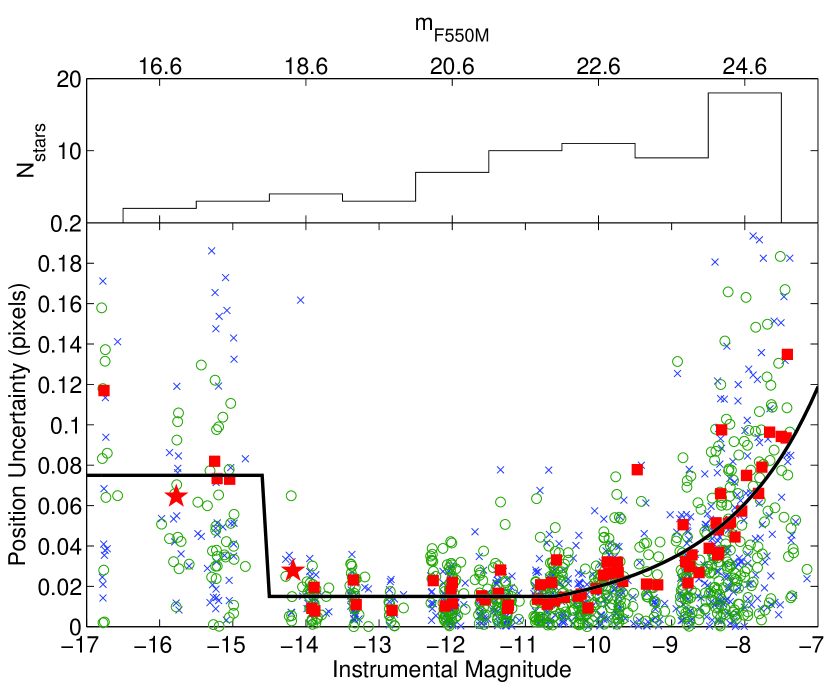
Refer to caption — Figure 1.— Bottom panel: Position uncertainty for each star as a function of instrumental magnitude ( $-2.5\log_{10}\mbox{Counts}$ in a $5\times 5\,$ pixel box) for the ACS/WFC data. The crosses are the $x$ position residuals, and open circles are the $y$ residuals, and the filled squares are the standard deviations of $x$ and $y$ combined, all divided by $\sqrt{2}$ so as to be appropriate for a single observation. The solid line is the uncertainty model derived in § 2.1. The Crab pulsar is the object at instrumental magnitude of $-15.8$ and our primary reference star (#4) is the object at $-14.1$ , both with a red stars. Top panel: number of stars used as a function of $m_{\rm F550M}$ , where we have taken $m_{\rm F550M}=m_{\rm inst}+32.6$ . The abscissae of the two panels are aligned.

For the WFPC2 data, we started with the trend found in Kaplan, van Kerkwijk, & Anderson (2002), and we used the same trend for uncertainty in pixels as a function of magnitude for both the PC and WF3. We then followed the procedure outlined above, although we found that we had to multiply the trend for the WF3 data by a factor⁴⁴4Since the trend was derived for the PC it is not surprising that its absolute scale should be different for the WF chips, but the shape seems consistent. of 1.5. For the saturated stars, which had $m_{\rm inst}<-10$ , we increased the uncertainty to 0.1 pixel for the PC and 0.15 pixel for WF3.

For both the ACS and WFPC2 data, we used the fits for the uncertainties as a function of magnitude rather than the actual uncertainty for each star as the measured uncertainty is estimated from only a few measurements and is therefore noisy, while the fit is more predictable. Kaplan et al. (2007) experimented in detail with different types of uncertainties and found that they largely did not affect the final results.

2.2. Near-IR Color-Magnitude Diagram

The interpretation of our results depends critically on the distances of the field stars to which we reference the Crab pulsar’s proper motion. We have thus derived a color-magnitude diagram of stars near the pulsar, using near-IR photometric observations with the Wide Field Infrared Camera (WIRC; Wilson et al. 2003) on the Palomar 200-inch telescope. The observations were on 2003 November 19, and we exposed for $15\times 20\,$ s in the $J$ and $K_{s}$ filters. The seeing was not very good, and averaged $1\farcs 5$ . For the reduction, we subtracted dark frames, then produced a sky frame for subtraction by taking a sliding box-car window of 4 exposures on either side of a reference exposure. We then added the exposures together, identified all the stars, and produced masks for the stars that were used to improve the sky frames in a second round of sky subtraction. We referenced the astrometry and photometry to the Two Micron All Sky Survey (2MASS; Skrutskie et al. 2006), using $>200$ well-detected stars that were not knots of nebulosity.

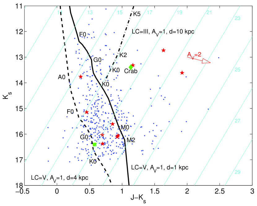
We used sextractor (Bertin & Arnouts, 1996) to produce a source list for the $K_{s}$ -band image, and then ran sextractor again on the $J$ -band image using the $K_{s}$ -band source list as a set of starting positions. Finally, we produced the color-magnitude diagram shown in Figure 2.

Given the depth of the images and the poor seeing, we could not measure near-IR magnitudes for most of the stars that we used for astrometry. These stars were mostly within the Crab nebula and the high background limited the ground-based image. Therefore our color-magnitude diagram predominantly includes stars from the full $8\arcmin\times 8\arcmin$ field outside the Crab nebula. We do not expect that the different astrometric and photometric samples will be biased relative to one another, except that the limiting magnitude in the near-IR is brighter: the photometric stars are those that are either very bright and/or are outside the Crab nebula, while the astrometric stars include those inside the nebula for a range of brightnesses. We estimated a rough conversion between our near-IR photometry and our HST photometry using synphot for $A_{V}=1.0\,$ mag, where we find $V-K_{\rm s}\approx 4.3(J-K_{\rm s})$ and $V\approx m_{\rm F550M}\approx m_{\rm F547M}$ (since the STMAG system is based on the Vega system at $V$ , no zeropoint offset is necessary). A rough photometric calibration for the HST data can be done with the instrumental magnitudes that we measure, such that $m_{\rm F550M}\approx m_{\rm inst}+32.6$ , where we neglect any aperture corrections. As can be seen from Figure 1, the majority of the stars are at $m_{\rm F550M}\gtrsim 21$ , which is fainter than most stars in Figure 2 but does not imply drastically different distances. The WFC saturation limit of $m_{\rm inst}=-14$ translates to $m_{\rm F550M}\approx 19$ , and indeed the stars above this line in Figure 2 are saturated.

From this we see that the majority of the stars in this field are consistent with main-sequence stars at distances of 1–4 kpc; a few may be more distant giants, and some of the astrometric reference stars may be among these, but they could also be slightly more reddened main-sequence stars (note that we are not accounting for the effects of metallicity). There should not be many stars that are much closer, as they would have to be rather redder than the more distant stars that we measure.

2.3. Fitting for the Astrometric Parameters

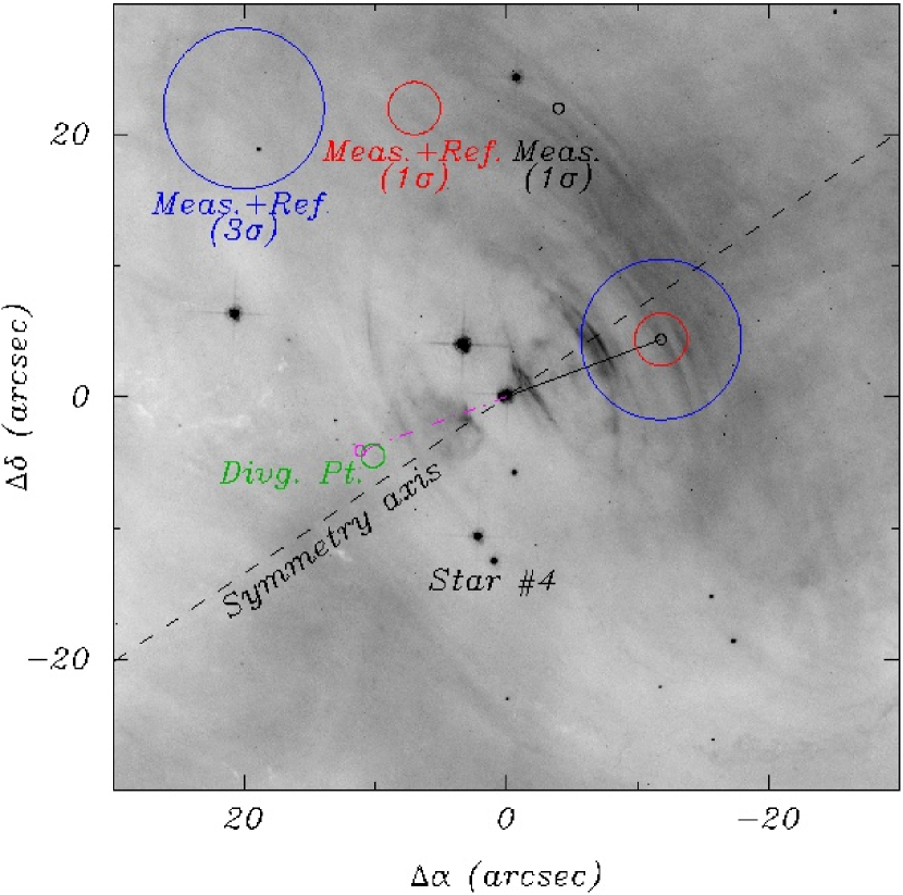
Once we have our data set with uncertainties as derived in § 2.1, we are in a position to fit for the positions and proper motions of each star, as well as the plate-scales, orientations, and central position of each exposure (see Kaplan et al. 2007 for a detailed description of the fitting procedure). For the fitting, we need to set the absolute plate-scale and orientation, which we did by assuming the plate-scale and orientation from the first exposure from pair 35 are the nominal values of $50\,\mbox{mas}\,\mbox{yr}^{-1}$ and the rotation from the image header; this exposure is no more likely than any other to have the correct plate-scale or orientation, but that will just lead to absolute uncertainties on the proper motion of $0.1$ % or less⁵⁵5We have verified this by fitting our final reference positions to positions derived from the WIRC data, which are referenced to 2MASS, which is tied to the International Coordinate Reference System. We find rotations of $<0.1\arcdeg$ and scale changes of $<0.1$ %. Also see § 2.4 and van der Marel et al. (2007).. We then also assumed that the orientation of the first exposure from pair 36 is the header value, since without two exposures with known orientations the fitting procedure could lead to a net rotation of the data with time that is compensated by a bulk proper motion. The fitting process might also compensate for a secularly increasing offset between exposures by introducing a fictitious bulk proper motion for the ensemble of stars. In order to prevent this, we initially assigned a star to have zero proper motion. This does not actually define the reference frame, since we can arbitrarily shift the proper motions of all of the stars. For this fixed star we chose #4 from NR06: this star has the advantage that it is close to the Crab pulsar, so it is on almost all exposures (73 of 94, after rejecting individual measurements for cosmic rays as described above) and is bright but not saturated (see Fig. 3). From § 2.2 and Figure 2 star #4 appears to be roughly at $\sim 4\,$ kpc.

Once we have measured source positions and estimated uncertainties at each epoch, we directly use the different observations to measure a proper motion. We fit simultaneously for the positions and proper motions of each star (with the proper motion of #4 fixed to zero) and the transformation parameters for each exposure (with the rotations and plate-scales fixed as discussed above for the first exposures in pairs 35 and 36), including all of the WFPC2 and ACS data in the fit. Each exposure had a 6-parameter transformation, such as that used by Kaplan et al. (2007) and Anderson & King (2006). Such a transformation is able to deal implicitly with linear variations in the distortion caused by breathing or systematic effects (Anderson, 2007). For the ACS data the fits give scale uncertainties of $\approx 0.0005$ % and position angle uncertainties of $0\fdg 0003$ , and shift uncertainties of $<0.01\,$ pixel. For the WFPC2 data the results are somewhat worse, largely due to the smaller number of stars: WF3 has scale uncertainties of $\approx 0.02$ % and position angle uncertainties of $0\fdg 005$ , and shift uncertainties of 0.02–0.1 pixel (depending on the number of stars included), while the PC has scale uncertainties of $\approx 0.07$ %, rotation uncertainties of $0\fdg 05$ , and shift uncertainties of $0.1\,$ pixel.

Initially we achieved a reasonable fit, with $\chi^{2}=5935.9$ for 3808 degrees of freedom (dof; we had 2322 observations of both $x$ and $y$ for 4644 data points, and 836 free parameters), or $\chi^{2}_{\rm red}=1.559$ . This $\chi^{2}$ results from comparing the computed positions of every star at every epoch (based on the fitted reference positions, proper motions, and frame transformations) to the measured positions; see Kaplan et al. (2007), Eqn. A6. However, there were anomalously large contributions to the total $\chi^{2}$ from a few deviant data points. Beyond the cosmic-ray rejections discussed above, we rejected an additional 8 measurements that deviated by more than $10\sigma$ from the best-fit model, and reduced $\chi^{2}$ to 4473.7 for 3792 dof ( $\chi^{2}_{\rm red}=1.180$ ; the proper motion of the pulsar changed by $\ll 1\sigma$ after the rejections). The rejected measurements were distributed among the stars and exposures, and likely represented statistical fluctuations or undetected cosmic-rays. After the additional rejections, the fit looked good overall, with no individual star or exposure dominating the fit. Note that the pulsar is saturated, and so its astrometric position uncertainty is significantly higher than most of the reference stars. As such, it does not dominate the overall fit. We tested using other reference stars and exposures (both ACS and WFPC2 observations), and the results did not depend on those choices except for a net shift in the proper motion, but we correct for this below.

As discussed above, all of the proper motions that we fit for are relative to that of star #4 from NR06, but we of course do not know what the proper motion of star #4 is, and it does not make a useful reference frame: with a transverse velocity dispersion of $\sim 20\,\mbox{km}\,\mbox{s}^{-1}$ and a distance of a few kpc, the proper motions of random stars are $\sim 1\,\mbox{mas}\,\mbox{yr}^{-1}$ . We must therefore try to determine a reference frame for our measurements in which the projected motion of the pulsar can be compared sensibly with the projected orientation of the nebular symmetry axis. We do so in two steps. First, we determine the average proper motion of the ensemble of reference stars. Next, we consider how those stars are moving relative to the Sun.

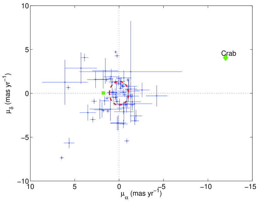
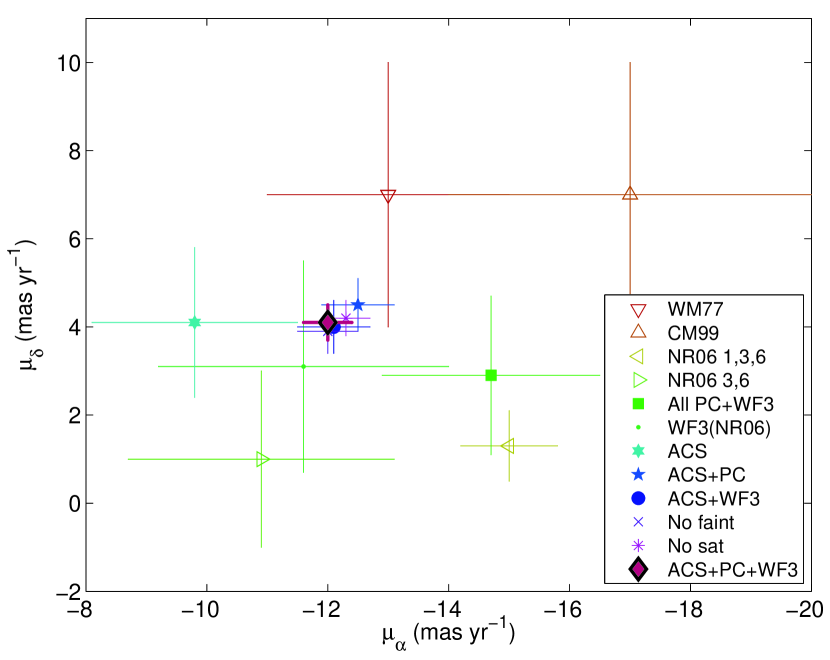
In Figure 4 we plot all of the proper motions that we measure. The Crab pulsar clearly has a much larger and more significant proper motion than the other objects, although we find a number of other stars with $>3\sigma$ detections of proper motion. In that figure we have determined the mean proper motion of all of the stars excluding the Crab pulsar (iteratively rejecting outliers) and shifted the proper motions to have zero mean. This shift has a magnitude of $(\Delta\mu_{\alpha},\Delta\mu_{\delta})=(-1.8\pm 0.2,-0.0\pm 0.2)\,\mbox{mas}\,\mbox{yr}^{-1}$ , moving star #4 to its position away from the origin. The circle in Figure 4 shows the standard deviation of the proper motions, and it is comparable to the magnitude of the shift. The uncertainty in the shift is much smaller, though, since it is the standard deviation divided by the square root of the number of stars used (here 49), and the shift in Right Ascension, at least, is statistically significant.

To see how our results depended on the choices of reference star/epochs, and on the datasets we used, we made a number of different fits. Using the whole ACS+WFPC2 dataset we iterated among a variety of reference stars, choosing ones that were relatively bright but not saturated and were close to the pulsar. We also used different ACS reference exposures and found that the proper motion values (corrected to have zero net stellar proper motion) changed by at most $0.6\,\mbox{mas}\,\mbox{yr}^{-1}$ , consistent with our uncertainties given below in Equation 2.

Table 2Measured Proper Motions for the Crab Pulsar

Reference	Data Source	Data Subsets	$\mu_{\alpha}$		$\mu_{\delta}$
			$(\mbox{mas}\,\mbox{yr}^{-1})$
WM77	Plates	$\cdots$	$-13$ $\pm$	2	$+7$ $\pm$	3
CM99	Limited HST WFPC2	$\cdots$	$-17$ $\pm$	3	+7 $\pm$	3
NR06	HST WFPC2	NR06 groups 1, 3, 6	$-15$ $\pm$	0.8	+1.3 $\pm$	0.8
NR06	HST WFPC2	NR06 groups 3, 6	$-10.9$ $\pm$	2.2	+1.0 $\pm$	2.0
This work	HST WFPC2	All PC+WF3	$-15.6$ $\pm$	1.8	$+3.7$ $\pm$	1.7
This work	HST WFPC2	NR06 groups 1, 3, 6	$-13.0$ $\pm$	2.4	+4.6 $\pm$	2.3
This work	HST ACS	$\cdots$	$-9.8$ $\pm$	1.7	+4.2 $\pm$	1.8
This work	HST ACS+WFPC2	All PC	$-12.5$ $\pm$	0.6	$+4.1$ $\pm$	0.6
This work	HST ACS+WFPC2	All WF3	$-12.1$ $\pm$	0.6	$+4.5$ $\pm$	0.6
This work	HST ACS+WFPC2	No faint stars^a^aWe rejected the 27 stars with $m_{\rm inst,F550M}>-9.5$ (the upward part of the trend in Fig. 1).	$-12.0$ $\pm$	0.5	$+3.9$ $\pm$	0.5
This work	HST ACS+WFPC2	No saturated stars^b^bWe rejected the four saturated reference stars. This also required removing several of the PC epochs since they had too few stars for proper solutions.	$-12.3$ $\pm$	0.4	+4.2 $\pm$	0.4
This work	HST ACS+WFPC2	$\cdots$	$-12.0$ $\pm$	0.4	$+4.1$ $\pm$	0.4

Note. — All proper motions are the values from fitting before correction for Solar motion or Galactic rotation. Proper motions from this work and WM77 are explicitly in a reference frame defined by the background stars in this field; CM99 explicitly assumes that the stars have zero proper motion. Also see Figure 5.

We then tried to choose different data sets, restricting ourselves to only the ACS data, only the WFPC2 data, only the WFPC2 data used by NR06, and some other combinations. In particular, we fit using none of the stars with instrumental magnitudes (from the ACS data) fainter than $-9.5$ : this excludes the portion of Figure 1 where the trend of uncertainty vs. magnitude climbs upwards. We also fit excluding all of the saturated stars from the ACS data, with the exception of the Crab pulsar (of course): this fit required us to remove some of the PC epochs, as without the saturated stars there were too few reference stars for a constrained fit. Such fits proceeded in exactly the same manner as the fit described above, with the only difference being that we used different observations as the initial reference; no other special manipulation was required for these fits. We found that the corrected proper motions from all of these data sets were consistent with each other, as listed in Table 2 and shown in Figure 5, but were not necessarily consistent with the values from the literature. Our result using just the data from NR06 was consistent with their result, although it had significantly higher uncertainties. This is because we took an uncertainty of 0.15 pix for the WF3 observations of the pulsar, which is 15 mas, while Figure 3 of NR06 shows their individual data points as having uncertainties of 5–8 mas. In contrast, our measurements using a longer time baseline and with the higher-precision ACS data were not consistent with the NR06 values. In all of these fits the resulting $\chi^{2}$ values were close to 1.0, indicating that our uncertainty estimates (§ 2.1) — which we derived just by comparing pairs of observations — were reasonable for the dataset as a whole, and gave good values for the different instruments. The fits that excluded the faint or the saturated reference stars could be used as our “default” fits, but we chose to retain as many stars as possible. With the exception of the PC epochs, where there are few stars, the saturated stars largely ride along with the fit and contribute very little, but they allow us to examine the goodness-of-fit for saturated objects besides the Crab pulsar, and indeed we find that the data fit them reasonably well (reduced $\chi^{2}$ of 0.85 to 1.48). The fainter stars contribute more to the fit, but are not dominant, and they allow us to examine the quality of the fit for a larger number of objects (again, it is good).

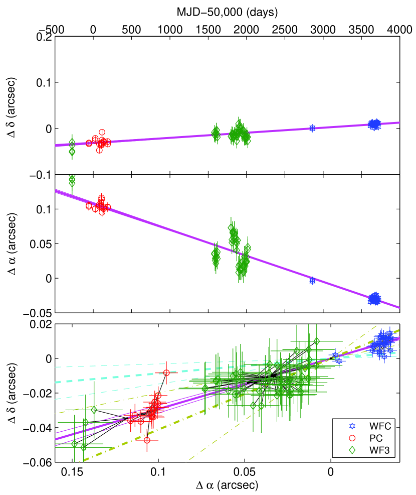
Using all of the data and our standard choices for reference exposures/star, the proper motion for just the Crab pulsar was a good fit, with $\chi^{2}_{\rm red}=217.3/184=1.18$ , although this $\chi^{2}$ is not formally correct as the parameters for the exposures are not properly counted. We show the astrometry in Figure 6. From this one can see that some pairs of exposures seem to deviate systematically from the overall trend, such as some of the WFPC2 data from near MJD 51,800. These are likely related to the changes in position angle of the observations (Tab. 1), although whether it is an intrinsic effect of the position angle (i.e. uncorrected distortion, perhaps related to charge transfer efficiency; Kozhurina-Platais, Goudfrooij, & Puzia 2007) or something to do with the changing set of reference stars, we cannot determine. Overall, though, the deviations are not greatly significant, and the proper motion is confirmed by our analyses of various subsets of the data. The corrected proper motion is:

	$\displaystyle\mu_{\alpha}$	$\displaystyle=$	$\displaystyle-12.0\pm 0.4\,\mbox{mas}\,\mbox{yr}^{-1}$
	$\displaystyle\mu_{\delta}$	$\displaystyle=$	$\displaystyle\phantom{0}\mbox{+4.1}\pm 0.4\,\mbox{mas}\,\mbox{yr}^{-1},$		(2)

where the uncertainty is a combination of the uncertainty on the derived proper motion and the uncertainty in the shift to the reference frame. This proper motion is in a reference frame defined by the average motion of the background stars in the field (this is the same procedure used for the initial measurement of WM77, which is their Equation 2, but the different choices of references stars means that the reference frames will not be exactly the same). However, as we discuss below, this reference frame is not the appropriate one for considering the degree of alignment between the pulsar motion and the projected symmetry axis of the surrounding nebula.

2.4. Absolute Position

We can get a position for the Crab pulsar tied to the International Celestial Reference System (ICRS; useful for analysis of timing data, for example) directly from 2MASS, which is tied to the ICRS⁶⁶6See http://spider.ipac.caltech.edu/staff/hlm/2mass/overv/overv.html. to better than $0\farcs 1$ . The pulsar is listed as source 2MASS J05343194+2200521, at position (J2000):

	$\displaystyle\alpha$	$\displaystyle=$	$\displaystyle 05^{\rm h}34^{\rm m}31\fs 94$
	$\displaystyle\delta$	$\displaystyle=$	$\displaystyle+22\arcdeg 00\arcmin 52\farcs 1,$		(3)

with quoted uncertainties of $\pm 0\farcs 06$ on each coordinate. This position has been precessed to equinox J2000, but it was actually measured on 1997 October 18. The 2.2 years between those dates implies a shift due to the measured proper motion of 27 mas, which is smaller than the measurement uncertainty. To verify the tie of the 2MASS data to the ICRS, we compared the position of 32 stars located within $5\arcmin$ of the pulsar that were detected in both 2MASS and the Second U. S. Naval Observatory CCD Astrograph Catalog (UCAC2; Zacharias et al. 2004), which is tied directly to the ICRS. We find a small residual shift ( $\approx 32\,$ mas) between 2MASS and UCAC2 (the UCAC2 proper motions for these stars are not statistically significant, so we did not include them), but this is again smaller than the measurement error reported by 2MASS. The 2MASS position is consistent with the radio imaging position (Han & Tian, 1999) listed in SIMBAD from the NRAO VLA Sky Survey (NVSS; Condon et al. 1998), but should be more accurate. A caveat, though, is that 2MASS could not measure the pulsar separately from the optical/infrared knot located $0\farcs 7$ away (Hester et al., 1995). However, the pulsar is $>40$ times brighter than the knot (at least at 5500 Å), and so the 2MASS centroid should essentially be at the pulsar’s position.

2.5. Proper Motion Reference Frame

Equation 2 gives the proper motion of the Crab pulsar relative to an ensemble of stars. Normally, we would correct our measured proper motion for the peculiar velocity of the Sun relative to the local standard of rest (LSR; we take the Solar motion to be $[U,V,W]_{\odot}=[10.00,5.25,7.17]{\rm~{}km\,s^{-1}}$ , where the uncertainties on those components are negligible compared to the other uncertainties discussed below; Dehnen & Binney 1998) and for the effects of differential Galactic rotation (DGR; we use the Galactic potential model of Kuijken & Gilmore 1989 to determine the rotation curve, and then examine deviations from the rotation curve determined by Brand & Blitz 1993), so that the proper motion reflects a velocity relative to the object’s local standard of rest. However, we should not apply these corrections blindly for the Crab pulsar. The reason is that the astrometric reference stars that we are using are at distances of 1–4 kpc (and possibly a bit further), comparable with the nominal 2 kpc distance of the Crab pulsar (§ 2.2). To first order, then, we do not need to correct for DGR or LSR motion.

To see how valid this is, we refine our distance estimate by following WM77. They found a mean statistical parallax of 0.5 mas for the reference stars from kinematic constraints, roughly consistent with our estimate of 1–4 kpc distances for the WIRC stars. Indeed, the stars used by WM77 were spread over several arcminutes and therefore are more comparable to the near-IR sample than the HST sample. WM77 formed their estimate by examining the dispersion of the reference stars about their mean proper motion and then relating that to the expected velocity dispersion. We find a proper motion dispersion of $\sigma_{\mu}=1.8\,\mbox{mas}\,\mbox{yr}^{-1}$ . Comparing this to the expected 1-D velocity dispersion of $32\,\mbox{km}\,\mbox{s}^{-1}$ (appropriate for late-type main-sequence stars; Binney & Merrifield, 1998, p. 632), we find a mean distance of 3–4 kpc, consistent with our photometric estimates and with the likelihood that some of the HST stars are fainter and more distant than the near-IR stars.

Of course, the stars are not all at a single distance, but are distributed over a range, and their contribution to the ensemble’s proper motion depends on their brightnesses and on how many observations we have for them. The range of distances will influence the ensemble’s mean proper motion: going from 1 kpc to 4 kpc increases the correction due to DGR by $0.2\,\mbox{mas}\,\mbox{yr}^{-1}$ , while the correction for the LSR decreases in magnitude by $1\,\mbox{mas}\,\mbox{yr}^{-1}$ . Since the Crab pulsar is toward the anti-center the LSR correction is more significant, and it depends inversely on distance. We take the pulsar to be at 2 kpc, which gives corrections of

	$\displaystyle(\Delta\mu_{\ell},\Delta\mu_{b})_{\rm DGR}(2\,\mbox{kpc})$	$\displaystyle=$	$\displaystyle(+0.68,+0.04)\,\mbox{mas}\,\mbox{yr}^{-1}$
	$\displaystyle(\Delta\mu_{\ell},\Delta\mu_{b})_{\rm LSR}(2\,\mbox{kpc})$	$\displaystyle=$	$\displaystyle(+0.47,-0.64)\,\mbox{mas}\,\mbox{yr}^{-1}.$		(4)

For the average stellar frame at 4 kpc, the corrections are:

	$\displaystyle(\Delta\mu_{\ell},\Delta\mu_{b})_{\rm DGR}(4\,\mbox{kpc})$	$\displaystyle=$	$\displaystyle(+0.78,+0.03)\,\mbox{mas}\,\mbox{yr}^{-1}$
	$\displaystyle(\Delta\mu_{\ell},\Delta\mu_{b})_{\rm LSR}(4\,\mbox{kpc})$	$\displaystyle=$	$\displaystyle(+0.23,-0.32)\,\mbox{mas}\,\mbox{yr}^{-1},$		(5)

so the net corrections are

	$\displaystyle(\Delta\mu_{\ell},\Delta\mu_{b})_{\rm DGR}(4\mbox{\,kpc}\rightarrow 2\,\mbox{kpc})$	$\displaystyle=$	$\displaystyle(-0.10,+0.01)\,\mbox{mas}\,\mbox{yr}^{-1}$
	$\displaystyle(\Delta\mu_{\ell},\Delta\mu_{b})_{\rm LSR}(4\,\mbox{kpc}\rightarrow 2\,\mbox{kpc})$	$\displaystyle=$	$\displaystyle(+0.24,-0.32)\,\mbox{mas}\,\mbox{yr}^{-1}.$

In equatorial coordinates these corrections are

	$\displaystyle(\Delta\mu_{\alpha},\Delta\mu_{\delta})_{\rm DGR}(4\mbox{\,kpc}\rightarrow 2\mbox{\,kpc})$	$\displaystyle=$	$\displaystyle(-0.05,+0.09)\,\mbox{mas}\,\mbox{yr}^{-1}$
	$\displaystyle(\Delta\mu_{\alpha},\Delta\mu_{\delta})_{\rm LSR}(4\mbox{\,kpc}\rightarrow 2\mbox{\,kpc})$	$\displaystyle=$	$\displaystyle(-0.14,-0.37)\,\mbox{mas}\,\mbox{yr}^{-1}.$

These corrections must be subtracted from the proper motion we found in § 2.3, so the proper motion of the pulsar relative to its local standard of rest is $\mu_{\alpha}=-11.8\,\mbox{mas}\,\mbox{yr}^{-1}$ , $\mu_{\delta}=+4.4\,\mbox{mas}\,\mbox{yr}^{-1}$ . Of course, these distances are uncertain. Assuming a 0.5 kpc uncertainty in the distance to the pulsar, and considering the range of 3 kpc to 5 kpc for the reference stars, we found that the correction overall varied by $\pm 0.1\,\mbox{mas}\,\mbox{yr}^{-1}$ from the nominal values in Equation LABEL:eqn:corr, so compared to the other sources of uncertainty this is a minor effect. We note that the uncertainties here exceed formal 1- $\sigma$ confidence intervals, since the distance intervals represent the full range of plausible distances. We also note that we have chosen a particular formulation of the Galactic rotation curve through the potential of Kuijken & Gilmore (1989): other formulations (flat rotation curves, use of Oort constants, etc.) give slightly different results for the DGR corrections. In particular, without a velocity that varies as a function of distance, the correction from $4\,$ kpc to $2\,$ kpc is identically 0. Using other choices (e.g., the rotation curve of Brand & Blitz 1993) changes the correction by a small amount on an absolute scale, typically $\pm 0.1\,\mbox{mas}\,\mbox{yr}^{-1}$ (other determinations of the LSR corrections agree to within 10%). We include this as an additional uncertainty.

However, more significant uncertainties come from our assumption that the rotation curve toward the outer Galaxy is both well-known and well-behaved, when it is neither. Overall, the rotation curve of the outer Galaxy has line-of-sight random variations of $\pm 5\,\mbox{km}\,\mbox{s}^{-1}$ (Brand & Blitz, 1993, and references therein), which accounts for the deviations of individual locations from the bulk velocity. The curve itself is poorly measured toward the anticenter, but this value should be relatively independent of position. So we would expect 1-D variations of $\pm 5\,\mbox{km}\,\mbox{s}^{-1}$ on top of the circular velocity, implying a proper motion uncertainty of $0.5\,\mbox{mas}\,\mbox{yr}^{-1}$ at 2 kpc. The proper motion is

	$\displaystyle\mu_{\alpha}$	$\displaystyle=$	$\displaystyle-11.8\pm 0.4\pm 0.5\,\mbox{mas}\,\mbox{yr}^{-1}$
	$\displaystyle\mu_{\delta}$	$\displaystyle=$	$\displaystyle\phantom{0}\mbox{+4.4}\pm 0.4\pm 0.5\,\mbox{mas}\,\mbox{yr}^{-1},$		(8)

compared to the local standard of rest of the Crab pulsar, where the first uncertainty is the measurement uncertainty (Eqn. 2) and the second is from the reference frame uncertainties.

Now, if our goal is to compare the proper motion vector to the projected orientation of the torus axis, we need to account for yet another zero point uncertainty, namely the unknown velocity of the Crab’s progenitor. The progenitor was presumably not stationary with respect to the local standard of rest at that position, and any peculiar velocity should remain after the explosion. Therefore a final zero-point uncertainty comes from the unknown peculiar velocity of the Crab pulsar’s progenitor. First, there are bulk streaming motions in the outer Galaxy with line-of-sight magnitude $\approx 12\,\mbox{km}\,\mbox{s}^{-1}$ (Brand & Blitz, 1993). Beyond this, early-type stars have 1-D velocity dispersions of $\sim 10\,\mbox{km}\,\mbox{s}^{-1}$ (Binney & Merrifield, 1998). Together these give into a 1-D velocity uncertainty of $16\,\mbox{km}\,\mbox{s}^{-1}$ , which, combined with the $0.5\,\mbox{mas}\,\mbox{yr}^{-1}$ uncertainty discussed above, translates into an uncertainty of $1.7\,\mbox{mas}\,\mbox{yr}^{-1}$ at 2 kpc, with a range of 1.4–2.3 $\,\mbox{mas}\,\mbox{yr}^{-1}$ for a distance range of 1.5–2.5 kpc (i.e. an uncertainty on the uncertainty). We assign a conservative value of $2.0\,\mbox{mas}\,\mbox{yr}^{-1}$ (considering the uncertainty on the distance as well as the reference frame velocities) for the systematic uncertainty due to combination of the reference frame effects, but also note that the progenitor’s velocity could have been much larger (see below). We then find a proper motion in the reference frame of the progenitor star of:

	$\displaystyle\mu_{\alpha}$	$\displaystyle=$	$\displaystyle-11.8\pm 0.4\pm 2.0\,\mbox{mas}\,\mbox{yr}^{-1}$
	$\displaystyle\mu_{\delta}$	$\displaystyle=$	$\displaystyle\phantom{0}\mbox{+4.4}\pm 0.4\pm 2.0\,\mbox{mas}\,\mbox{yr}^{-1},$		(9)

where again the two uncertainties are from the measurement and the unknown reference frame, as discussed above. This proper motion has a magnitude of $\mu=12.5\pm 0.4\pm 2.0\,\mbox{mas}\,\mbox{yr}^{-1}$ at an angle of $290\arcdeg\pm 2\arcdeg\pm 9\arcdeg$ (east of north), or a transverse velocity of $120\,\mbox{km}\,\mbox{s}^{-1}$ for a distance of 2 kpc; the velocity is quite uncertain, both due to the uncertain frame of the proper motion and the distance uncertainty.

3. Discussion and Conclusions

While we assumed a velocity of $\pm 10\,\mbox{km}\,\mbox{s}^{-1}$ for the Crab pulsar’s progenitor, it is possible that the progenitor itself had a much larger space velocity. This was proposed early on by Minkowski (1970), who considered the high proper motion of the pulsar to be a relic of the progenitor’s velocity and that the progenitor itself was a runaway star (e.g., Blaauw 1961) from the Gem OB1 association. However, Minkowski (1970) later dismissed this hypothesis since he did not believe that the supernova was a type II explosion. Gott et al. (1970) have a similar idea, where they consider the Crab pulsar and the nearby pulsar B0525+21 (two of the first pulsars to be discovered; Staelin & Reifenstein 1968) as former binary companions ejected from the Gem OB1 association; Harrison et al. (1993) attempted to measure the proper motion of PSR B0525+21 but did not find a statistically significant result. Later analyses, such as Pols (1994) and Mdzinarishvili & Dzigvashvili (2001), have revived the hypothesis that the progenitor had a large ( $>100\,\mbox{km}\,\mbox{s}^{-1}$ ) space velocity, with Pols (1994) arguing that the large height below the Galactic plane (200 pc for a distance of 2 kpc, which is larger than the scale-height of OB stars; Reed 2000; Elias, Cabrera-Caño, & Alfaro 2006) and the presumed evolutionary state of the progenitor (inferred from the elemental and velocity structure of the Crab Nebula) suggest that the Crab pulsar was formed from the second explosion in a binary system, and that it had a large space velocity from the first explosion. Currently we cannot say definitively whether or not the progenitor had a significant space velocity and must therefore treat this as an overall uncertainty on our whole analysis.

3.1. Location of the Explosion Center

A number of authors have estimated the “divergent point” for the Crab Nebula: the point from which all of the filaments seem to traveling outwards, which is presumed to be the center of the explosion. Among the more reliable measurements are those of Trimble (1968), WM77, and Nugent (1998, who also review the situation), which we list in Table 3. Most of these determinations trace the filaments back and find best-fit dates for the explosion of $\approx 1130$ CE instead of the commonly accepted 1054 CE (Stephenson & Green, 2002), with the difference caused by unmodeled acceleration of the filaments.

Table 3Comparison Between Our Proper Motion and Divergent Points

Reference	Divergent Point (J2000)^a^aThe positions of the divergent point according to Trimble (1968) and Nugent (1998) were computed from the offsets given in Nugent (1998) between the divergent point/explosion center and the star $5\arcsec$ to the north-east of the pulsar, whose position we take to be: $\alpha=05^{\rm h}34^{\rm m}32\fs 17$ , $\delta=+22\arcdeg 00\arcmin 56\farcs 0$ from 2MASS (the star is 2MASS J05343217+2200560). For WM77, we take the divergent point directly from their paper (Eqn. 17).		Divg. Date^b^bDate of closest approach between our proper motion vector projected backwards and the divergent point. The uncertainties are only measurement uncertainties — no reference frame uncertainties are included.	$\Delta r_{\rm min}$ ^c^cClosest approach between our proper motion projected backward and the estimated divergent point of the filaments.	$\Delta r$ (1054 CE)^d^dDistance between our proper motion projected backward and the divergent point for 1054 CE.
	$\alpha$	$\delta$	(CE)	(arcsec)	(arcsec)
Trimble (1968)	$05^{\rm h}34^{\rm m}32\fs 72\pm 0\fs 12$	$+22\arcdeg 00\arcmin 47\farcs 5\pm 1\farcs 4$	$1067\pm 138$	$0.5$	0.6
WM77	$05^{\rm h}34^{\rm m}32\fs 67\pm 0\fs 06$	$+22\arcdeg 00\arcmin 47\farcs 6\pm 0\farcs 9$	$1114\pm 78$	0.7	1.0
Nugent (1998)	$05^{\rm h}34^{\rm m}32\fs 84\pm 0\fs 12$	$+22\arcdeg 00\arcmin 48\farcs 0\pm 1\farcs 3$	$947\pm 138$	0.6	1.5
This work^e^eNot truly a divergent point, but rather the location of the pulsar projected back to 1054 CE.	$05^{\rm h}34^{\rm m}32\fs 74\pm 0\fs 03$	$+22\arcdeg 00\arcmin 47\farcs 9\pm 0\farcs 4$	1054	$\cdots$	$\cdots$

With the proper motion that we derive, the explosion centers from the literature, and the nominal explosion date of 1054 CE, we can perform three tests: we have a time, a displacement, and a velocity, and we can use any two of those to estimate the third. First, we can measure how close our proper motion comes to the various explosion centers for the nominal explosion date, and we give these values in the last column (“ $\Delta r$ (1054 CE)”) of Table 3. Second, we can compute the dates of closest approach between our projected proper motion vectors and the explosion centers, which serve as our own estimates of the explosion dates. The uncertainties on those values are dominated by the uncertainties of the divergent point measurements ( $\sim 1\arcsec$ ), and the values are given in the “Divg. Date” column of Table 3, with the approach distances for those dates given in the “ $\Delta r_{\rm min}$ ” column. Finally, we can compute our own estimate for the explosion position, taking our proper motion and assuming the date of 1054 CE, and we give this in the last row of Table 3.

In general, all of the values — the approach distances for 1054 CE, the explosion dates, and our inferred explosion center — are consistent at better than 1- $\sigma$ . The first two elements are largely consistency checks: this shows that our proper motion is consistent with the independent divergent point estimates, and that our reference frame corrections are consistent (although they were not explicitly the same). As discussed in WM77, the location of the divergent point depends on the choice of reference frame, so we cannot address any of the larger reference frame uncertainties. We note, though, that in contrast to our proper motion that approaches the divergent points with distances of $<1\arcsec$ , the proper motion of NR06 does approximately a factor of 3 worse. The final element that we have computed, our own estimate for the explosion center, is more precise than previous estimates by a factor of $\sim$ 2–3 in each axis. This may serve to help constrain future measurements of the filament motions and acceleration, as its independence from the filaments themselves should improve the reliability of the measurements.

3.2. Spin-Kick MisAlignment

Ng & Romani (2004) fit a model to the torus seen in the HST data, and find a best-fit torus symmetry axis of $304.0\arcdeg\pm 0.1\arcdeg$ , which is the projection of the spin axis on the plane of the sky. This implies a projected misalignment of $14\arcdeg\pm 2\arcdeg\pm 9\arcdeg$ , as seen Figure 3. This projected misalignment is less than that found in NR06, and is significant if one only considers the measurement uncertainty: with all of the uncertainties, the misalignment is consistent with a broad range of values, including zero.

Perhaps the next best case of a pulsar wind nebula giving the projected spin axis is that of the Vela pulsar (catalog PSR B0833-45), where the proper motion (corrected for Galactic rotation and solar motion) is $45\pm 1.3\,\mbox{mas}\,\mbox{yr}^{-1}$ at a position angle of $301\arcdeg\pm 2\arcdeg$ (Dodson et al., 2003). The symmetry axis of the torus is at a position angle of $310.6\arcdeg\pm 0.1\arcdeg$ (Ng & Romani, 2004), giving the projected misalignment of $10\arcdeg\pm 2\arcdeg$ (Ng & Romani, 2007). For this system, the proper motion reference frame and corrections should be better defined than those for the Crab: the proper motion is measured in the radio, so the reference sources are at infinite distance; and the Vela pulsar is reasonably close (with a distance measured through geometric parallax) and not located at the Galactic anti-center, so the effects of Galactic rotation are much better understood. However, Ng & Romani (2004) still fail to include any allowance for the unknown velocity of the progenitor: a $\pm 10\,\mbox{km}\,\mbox{s}^{-1}$ velocity at a distance of $287\,$ pc is $\pm 7\,\mbox{mas}\,\mbox{yr}^{-1}$ (or an angular uncertainty of $\sim 9\arcdeg$ ), so again this completely dominates the measurement uncertainty and makes the degree of misalignment consistent with zero.

The two examples considered here, the Crab and Vela pulsars, while the two best X-ray tori (Ng & Romani, 2004), may not be good cases for computing misalignment. This is because they are both moving at smaller velocities than the average pulsar population ( $120\,\mbox{km}\,\mbox{s}^{-1}$ and $61\,\mbox{km}\,\mbox{s}^{-1}$ , vs. $\sim 400\,\mbox{km}\,\mbox{s}^{-1}$ ; e.g., Hobbs et al. 2005; Faucher-Giguère & Kaspi 2006), so the unknown velocity of the progenitor has a correspondingly greater contribution. In fact, there is a bias in favor of tori being found around relatively slow pulsars. This is because the transition from a “bubble” pulsar wind nebula (PWN) with a torus to a bow-shock PWN (see Gaensler & Slane, 2006) occurs when the pulsar has traveled roughly 68% of the distance from the center of the of the supernova remnant to its edge (van der Swaluw, Downes, & Keegan, 2004), largely independent of the pulsar’s velocity. So slower pulsars will spend longer in the bubble/torus phase. For faster moving pulsars, whose proper motions and projected spin axes are not as well determined (in general they are further away), the uncertainty will be closer to $1\arcdeg$ and will not dominate over the measurement uncertainties. In addition, if the model of Ng & Romani (2007) is correct, we would expect the faster moving pulsars to be intrinsically closer to alignment. We also note that, for pulsars moving at $>200\,\mbox{km}\,\mbox{s}^{-1}$ , all of the reference frame uncertainties discussed here will lead to uncertainties of $<10$ % on the space velocity: this will typically be less than the uncertainty on the distance. Therefore, in studying the magnitude of pulsar velocities (or of the pulsar population) the reference frame uncertainties will not be significant.

However, we can also look at the situation from the other side. If the spin and kick axes were perfectly aligned in the reference frame of the progenitor’s motion, we could still (erroneously) infer a misalignment because of a high progenitor space velocity. In practice, though, it is difficult to disentangle the effects of intrinsic and apparent misalignments for single objects. A further complication comes from the fact that all alignments are examined only in projection: inclinations of nebulae can be estimated (although not directly measured), but radial velocities of pulsars are entirely unknown, and without the third dimension any observed alignments could still be coincidences.

A number of other pulsar wind nebulae also have symmetry axes (e.g., Pavlov et al., 2001; Helfand et al., 2001; Ng & Romani, 2004), although the lower fluxes and larger distances make most of these hard to observe in detail. There are other situations where alignments are inferred but not measured directly: for instance, using an offset from the center of a supernova remnant to derive a kick direction (this approach can introduce substantial systematic errors of its own; see Gaensler et al. 2006), and deriving a rotation axis from fitting radio polarization data (Deshpande et al., 1999; Lai et al., 2001; Romani & Ng, 2003; Wang et al., 2006; Rankin, 2007). For those systems with constrained proper motions and rotations axes, Ng & Romani (2004) find projected misalignments of $\sim 10\arcdeg$ , although most are consistent with zero. Wang et al. (2006) and Ng & Romani (2007) find similar misalignments for a larger sample using polarization data (also see Deshpande et al. 1999), but especially if we restrict the sample to the younger pulsars (where Galactic acceleration should not have modified the initial velocity) then the conclusions are similar to Ng & Romani (2004) (also see Johnston et al. 2005). This suggests that, at least statistically, there still is a considerable degree of alignment between projected spin axes and proper motions. From this, Wang et al. (2007) and Ng & Romani (2007) argue that the asymmetries experienced by proto-neutron stars following core-collapse simultaneously can impart these stars with both kick and spin, and that these asymmetries consist of a stochastic ensemble of thrusts, each long enough to result in rotational averaging of the resultant linear momentum vector. The uncertainties discussed in this paper illustrate the difficulties in measuring precision alignments (or lack thereof) in any individual object. Further progress in these studies, for example, via detailed analyses of how the degree of alignment depends on parameters such as space velocity and surface magnetic field strength, is best achieved by adding to the total number of pulsars with information on the orientations of both spin and kick.

We thank a referee for a thorough reading, C.-Y. Ng for helpful comments, and M. Bietenholz for assistance in clarifying some of the reference frame issues. Support for this work was provided by the National Aeronautics and Space Administration through Hubble award AR-10667.01. Partial support for DLK was also provided by NASA through Hubble Fellowship grant #01207.01-A awarded by the Space Telescope Science Institute, which is operated by the Association of Universities for Research in Astronomy, Inc., for NASA, under contract NAS 5-26555. B. M. G. acknowledges the support of NASA through LTSA grant NAG5-13032. S. C. acknowledges support from the University of Sydney Postdoctoral Fellowship Program. This research has made use of the SIMBAD database, operated at CDS, Strasbourg, France. This research has made use of SAOImage DS9, developed by the Smithsonian Astrophysical Observatory. Facilities: Hale (WIRC), HST (WFPC2, ACS)

Appendix A Prospects for Parallax

Given the importance of the Crab pulsar in our understanding of neutron stars, its precise distance remains a surprisingly open question. A trigonometric parallax has not yet been measured for the pulsar. From the dispersion of its radio pulses and a model of the Galactic electron density distribution (NE2001, Cordes & Lazio, 2002), PSR B0531+21 has an inferred distance of 1.7 kpc (a distance range of 1.4—2.0 kpc). Trimble (1973) estimated a range of distances between 1.4 and 2.7 kpc based on a variety of lines of evidence, and the nominal distance to the Crab pulsar and its nebula is quoted as $2.0\pm 0.5\,$ kpc. Precise measurements of the times of arrival of radio pulses have been used to measure radio pulsar parallaxes, but such measurements require exceptional rotational stability, generally seen only in some recycled pulsars (e.g., PSR J0437 $-$ 4715; van Straten et al., 2001). The young Crab pulsar has noisy timing residuals and shows rotational glitches (Wong, Backer, & Lyne, 2001), ruling out such an approach to astrometry. Thus a parallax (and proper motion) for the Crab pulsar must rely on imaging at some wavelength range, and radio VLBI or optical observations with space telescopes are currently the most plausible approaches.

From a purely numerical perspective, it appears that one should be able to use HST observations of the Crab pulsar, as described in this work, to measure its parallax. After all, for bright stars the ePSF measurements and distortion solution are accurate to $0.01\,$ pixel in an individual exposure (Anderson & King, 2004, 2006; Kaplan et al., 2007), which is $0.25\,$ mas for the ACS/High Resolution Camera (HRC) and $0.5\,$ mas for the ACS/WFC. With its distance around 2 kpc, we expect a parallax near 0.5 mas, so with a sufficient number of exposures this should be measurable in principle. However, there are two limiting factors. First, it seems that for the brightest stars systematic effects prevent the combination of individual exposures from reducing the astrometric uncertainty by the square-root of the number of exposures as one might expect (see, e.g., Kaplan et al. 2007). Second, unlike in radio interferometry where the parallax is measured relative to quasars and radio galaxies at essentially “infinite” distance, we must measure relative to other stars in our Galaxy that are at finite distances. For our measurement of the parallax of a neutron star at $\approx 350\,$ pc (Kaplan et al., 2007), we found that most of the reference stars were at 1–2 kpc and therefore had parallaxes at the 0.5–1.0 mas level. If we had ignored them, our parallax measurement would have been biased by the weighted mean of the parallaxes of the reference stars, or $\approx 0.5\,$ mas, which is quite significant. Luckily, we had enough photometry of the field that we were able to determine photometric parallaxes for the reference stars. While not very accurate individually, they were sufficiently close to the true values (as we measured from our astrometry) to allow the correction of the ensemble of stars and the removal of the parallactic bias.

From our color-magnitude diagram, we see that the background stars for the Crab pulsar are largely at 1–4 kpc, although there may be some at larger distances. Therefore the mean parallax of the background sources is likely $\gtrsim 0.25\,$ mas, or approximately one half of the expected parallax of the Crab pulsar. This is a very significant correction and in order to measure the parallax of the pulsar with any significance we would need to know this bias to better than $10$ %. This might be possible with more detailed photometry (unfortunately, while the field is frequently observed by many facilities, most use narrow-band filters that are not suitable for spectral typing) or limited spectroscopy, but it would require a dedicated set of observations.

Overall, then, the prospects for an optical astrometric parallax do not seem to be very good. First, we would need a number of additional astrometric HST observations, likely with the ACS/HRC (again, this may not be possible due to the recent failure of this instrument), where the Crab pulsar is not saturated, but this will of course mean that we detect fewer reference stars (due both to the limited field of the ACS/HRC and the shallower exposures). Since we are worried about accuracy at the $<0.01\,$ pix level, we must also attempt to refine our estimate of the distortion solution and ePSF, which are difficult with relatively sparse fields like this one. We must also be confident in all of our systematics at this level. Second, we need a good number of multi-band photometric observations to measure reliable photometric parallaxes for at least the majority of the background stars; since we are observing out of the Galaxy, we must be able to distinguish between solar metallicity stars in the disk and low-metallicity stars in the halo. The upcoming Wide Field Camera 3 (WFC3) on HST will have Strömgren (1966) $uvby\beta$ filters that greatly aid in stellar typing, but this may not be enough. It is therefore our opinion that an optical parallax is unlikely with current instruments, although it may be possible with future instruments such as the Space Interferometry Mission or GAIA.

Very Long Baseline Interferometry (and specifically the Very Long Baseline Array) has been used to measure the proper motions and parallaxes of a number of neutron stars, including some which are both weaker and more distant than the Crab pulsar (see, e.g. Brisken et al., 2002; Chatterjee et al., 2005). Such observations would provide astrometry referenced to distant extragalactic quasars, eliminating uncertainty due to the reference frame (c.f. our discussion in §2.2, §2.5, and above), although we would still require DGR and LSR corrections. However, the Crab pulsar is embedded in an extremely radio-bright nebula, which dominates the system temperature of radio telescopes and thus limits the signal-to-noise ratio of radio interferometric observations. Coupled with the absence of a suitable extragalactic reference source nearby, the large increase in system temperature has limited attempts to measure a precise proper motion and parallax with the VLBA. Simply adding sensitivity (by increasing the collecting area, bandwidth, or integration time) does not address these limitations. We note that the $\sim$ 6′ size of the Crab nebula is comparable to the size of the primary beam of the 25-m VLBA antennas ( $\sim$ 9′ at 5 GHz). A telescope consisting of smaller dishes (such as the current Reference Design for the Square Kilometer Array⁷⁷7See SKA Memorandum #69 at http://www.skatelescope.org/PDF/memos/69_ISPO.pdf.) would have a wider field of view and suffer a proportionately smaller decrease in signal-to-noise ratio for the same total collecting area when observing a source as strong as the Crab nebula. The wider field of view and higher sensitivity would also provide suitable astrometric reference sources. Future radio telescopes with continent-sized baselines may thus enable a VLBI parallax for the Crab pulsar.

It is unfortunate that the Crab pulsar, a subject of such intense and detailed investigation for so long, remains just beyond our current astrometric capabilities. However, the next generation of optical and radio telescopes should allow the measurement of a trigonometric parallax to this object, finally settling questions about its distance.

References

Anderson (2007) Anderson, J. 2007, Variation of the Distortion Solution of the WFC, HST Instrument Science Report 07-08, Space Telescope Science Institute
Anderson & King (2004) Anderson, J. & King, I. 2004, Multi-filter PSFs and Distortion Corrections for the HRC, HST Instrument Science Report 04-15, Space Telescope Science Institute
Anderson & King (2006) —. 2006, PSFs, Photometry, and Astrometry for the ACS/WFC, HST Instrument Science Report 06-11, Space Telescope Science Institute
Anderson & King (2000) Anderson, J. & King, I. R. 2000, PASP, 112, 1360
Anderson & King (2003) —. 2003, PASP, 115, 113
Arras & Lai (1999) Arras, P. & Lai, D. 1999, ApJ, 519, 745
Arzoumanian et al. (2002) Arzoumanian, Z., Chernoff, D. F., & Cordes, J. M. 2002, ApJ, 568, 289
Bertin & Arnouts (1996) Bertin, E. & Arnouts, S. 1996, A&AS, 117, 393
Binney & Merrifield (1998) Binney, J. & Merrifield, M. 1998, Galactic Astronomy (Princeton, NJ: Princeton University Press)
Blaauw (1961) Blaauw, A. 1961, Bull. Astron. Inst. Netherlands, 15, 265
Brand & Blitz (1993) Brand, J. & Blitz, L. 1993, A&A, 275, 67
Brisken et al. (2002) Brisken, W. F., Benson, J. M., Goss, W. M., & Thorsett, S. E. 2002, ApJ, 571, 906
Brisken et al. (2003) Brisken, W. F., Fruchter, A. S., Goss, W. M., Herrnstein, R. M., & Thorsett, S. E. 2003, AJ, 126, 3090
Burrows & Hayes (1996) Burrows, A. & Hayes, J. 1996, Physical Review Letters, 76, 352
Burrows et al. (1995) Burrows, A., Hayes, J., & Fryxell, B. A. 1995, ApJ, 450, 830
Burrows et al. (2006) Burrows, A., Livne, E., Dessart, L., Ott, C. D., & Murphy, J. 2006, ApJ, 640, 878
Caraveo & Mignani (1999) Caraveo, P. A. & Mignani, R. P. 1999, A&A, 344, 367
Chatterjee et al. (2005) Chatterjee, S., et al. 2005, ApJ, 630, L61
Condon et al. (1998) Condon, J. J., Cotton, W. D., Greisen, E. W., Yin, Q. F., Perley, R. A., Taylor, G. B., & Broderick, J. J. 1998, AJ, 115, 1693
Cordes & Lazio (2002) Cordes, J. M. & Lazio, T. J. W. 2002, ArXiv e-print, astro-ph/0207156
Cowsik (1998) Cowsik, R. 1998, A&A, 340, L65
Cox (2000) Cox, A. N. 2000, Allen’s Astrophysical Quantities, 4th edn. (New York: AIP Press/Springer)
Dehnen & Binney (1998) Dehnen, W. & Binney, J. J. 1998, MNRAS, 298, 387
Deshpande et al. (1999) Deshpande, A. A., Ramachandran, R., & Radhakrishnan, V. 1999, A&A, 351, 195
Dodson et al. (2003) Dodson, R., Legge, D., Reynolds, J. E., & McCulloch, P. M. 2003, ApJ, 596, 1137
Elias et al. (2006) Elias, F., Cabrera-Caño, J., & Alfaro, E. J. 2006, AJ, 131, 2700
Faucher-Giguère & Kaspi (2006) Faucher-Giguère, C.-A. & Kaspi, V. M. 2006, ApJ, 643, 332
Fruchter & Mutchler (1998) Fruchter, A. & Mutchler, M. 1998, Space Telescope Science Institute Memo, 28 July
Gaensler et al. (2006) Gaensler, B. M., Chatterjee, S., Slane, P. O., van der Swaluw, E., Camilo, F., & Hughes, J. P. 2006, ApJ, 648, 1037
Gaensler & Slane (2006) Gaensler, B. M. & Slane, P. O. 2006, ARA&A, 44, 17
Gott et al. (1970) Gott, J. R. I., Gunn, J. E., & Ostriker, J. P. 1970, ApJ, 160, L91
Gunn & Ostriker (1970) Gunn, J. E. & Ostriker, J. P. 1970, ApJ, 160, 979
Han & Tian (1999) Han, J. L. & Tian, W. W. 1999, A&AS, 136, 571
Harrison et al. (1993) Harrison, P. A., Lyne, A. G., & Anderson, B. 1993, MNRAS, 261, 113
Helfand et al. (2001) Helfand, D. J., Gotthelf, E. V., & Halpern, J. P. 2001, ApJ, 556, 380
Hester et al. (2002) Hester, J. J., et al. 2002, ApJ, 577, L49
Hester et al. (1995) Hester, J. J., et al. 1995, ApJ, 448, 240
Hobbs et al. (2005) Hobbs, G., Lorimer, D. R., Lyne, A. G., & Kramer, M. 2005, MNRAS, 360, 974
Iben & Tutukov (1996) Iben, I. J. & Tutukov, A. V. 1996, ApJ, 456, 738
Janka & Mueller (1996) Janka, H.-T. & Mueller, E. 1996, A&A, 306, 167
Janka et al. (2005) Janka, H.-T., Scheck, L., Kifonidis, K., Müller, E., & Plewa, T. 2005, in Astronomical Society of the Pacific Conference Series, Vol. 332, The Fate of the Most Massive Stars, ed. R. Humphreys & K. Stanek (San Francisco: ASP), 363
Johnston et al. (2005) Johnston, S., Hobbs, G., Vigeland, S., Kramer, M., Weisberg, J. M., & Lyne, A. G. 2005, MNRAS, 364, 1397
Johnston et al. (2006) —. 2006, Chinese Journal of Astronomy and Astrophysics Supplement, 6, 237
Kaplan et al. (2002) Kaplan, D. L., van Kerkwijk, M. H., & Anderson, J. 2002, ApJ, 571, 447
Kaplan et al. (2007) —. 2007, ApJ, 660, 1428
Koekemoer et al. (2002) Koekemoer, A. M., Fruchter, A. S., Hook, R. N., & Hack, W. 2002, in The 2002 HST Calibration Workshop, ed. S. Arribas, A. Koekemoer, & B. Whitmore (Baltimore: Space Telescope Science Institute), 337
Kozhurina-Platais et al. (2007) Kozhurina-Platais, V., Goudfrooij, P., & Puzia, T. H. 2007, ACS/WFC:Differential CTE corretions for Photometry and Astrometry from non-drizzled images, HST Instrument Science Report 07-14, Space Telescope Science Institute
Kuijken & Gilmore (1989) Kuijken, K. & Gilmore, G. 1989, MNRAS, 239, 571
Lai et al. (2001) Lai, D., Chernoff, D. F., & Cordes, J. M. 2001, ApJ, 549, 1111
Lai & Goldreich (2000) Lai, D. & Goldreich, P. 2000, ApJ, 535, 402
Mdzinarishvili & Dzigvashvili (2001) Mdzinarishvili, T. & Dzigvashvili, R. 2001, Astrophysics, 44, 463
Minkowski (1970) Minkowski, R. 1970, PASP, 82, 470
Ng & Romani (2004) Ng, C.-Y. & Romani, R. W. 2004, ApJ, 601, 479
Ng & Romani (2006) —. 2006, ApJ, 644, 445
Ng & Romani (2007) —. 2007, ApJ, 660, 1357
Nugent (1998) Nugent, R. L. 1998, PASP, 110, 831
Pavlov et al. (2001) Pavlov, G. G., Kargaltsev, O. Y., Sanwal, D., & Garmire, G. P. 2001, ApJ, 554, L189
Pols (1994) Pols, O. R. 1994, A&A, 290, 119
Portegies Zwart & van den Heuvel (1999) Portegies Zwart, S. F. & van den Heuvel, E. P. J. 1999, New Astronomy, 4, 355
Rankin (2007) Rankin, J. M. 2007, ApJ, 664, 443
Reed (2000) Reed, B. C. 2000, AJ, 120, 314
Romani (2005) Romani, R. W. 2005, in Astronomical Society of the Pacific Conference Series, Vol. 328, Binary Radio Pulsars, ed. F. A. Rasio & I. H. Stairs (San Francisco: ASP), 337
Romani & Ng (2003) Romani, R. W. & Ng, C.-Y. 2003, ApJ, 585, L41
Scheck et al. (2006) Scheck, L., Kifonidis, K., Janka, H.-T., & Müller, E. 2006, A&A, 457, 963
Scheck et al. (2004) Scheck, L., Plewa, T., Janka, H.-T., Kifonidis, K., & Müller, E. 2004, Physical Review Letters, 92, 011103
Shklovskii (1970) Shklovskii, I. S. 1970, AZh, 46, 715
Skrutskie et al. (2006) Skrutskie, M. F., et al. 2006, AJ, 131, 1163
Socrates et al. (2005) Socrates, A., Blaes, O., Hungerford, A., & Fryer, C. L. 2005, ApJ, 632, 531
Sollerman et al. (2000) Sollerman, J., Lundqvist, P., Lindler, D., Chevalier, R. A., Fransson, C., Gull, T. R., Pun, C. S. J., & Sonneborn, G. 2000, ApJ, 537, 861
Spruit & Phinney (1998) Spruit, H. C. & Phinney, E. S. 1998, Nature, 393, 139
Staelin & Reifenstein (1968) Staelin, D. H. & Reifenstein, E. C. 1968, Science, 162, 1481
Stephenson & Green (2002) Stephenson, F. R. & Green, D. A. 2002, Historical supernovae and their remnants (Clarendon Press: Oxford)
Strömgren (1966) Strömgren, B. 1966, ARA&A, 4, 433
Trimble (1968) Trimble, V. 1968, AJ, 73, 535
Trimble (1973) —. 1973, PASP, 85, 579
van den Heuvel & van Paradijs (1997) van den Heuvel, E. P. J. & van Paradijs, J. 1997, ApJ, 483, 399
van der Marel et al. (2007) van der Marel, R. P., Anderson, J., Cox, C., Kozhurina-Platais, V., Lallo, M., & Nelan, E. 2007, Calibration of ACS/WFC Absolute Scale and Rotation for Use in Creation of a JWST Astrometric Reference Field, HST Instrument Science Report 07-07, Space Telescope Science Institute
van der Swaluw et al. (2004) van der Swaluw, E., Downes, T. P., & Keegan, R. 2004, A&A, 420, 937
van Straten et al. (2001) van Straten, W., Bailes, M., Britton, M., Kulkarni, S. R., Anderson, S. B., Manchester, R. N., & Sarkissian, J. 2001, Nature, 412, 158
Wang et al. (2006) Wang, C., Lai, D., & Han, J. L. 2006, ApJ, 639, 1007
Wang et al. (2007) —. 2007, ApJ, 656, 399
Wilson et al. (2003) Wilson, J. C., et al. 2003, Proc. SPIE, 4841, 451
Wong et al. (2001) Wong, T., Backer, D. C., & Lyne, A. G. 2001, ApJ, 548, 447
Wyckoff & Murray (1977) Wyckoff, S. & Murray, C. A. 1977, MNRAS, 180, 717
Zacharias et al. (2004) Zacharias, N., Urban, S. E., Zacharias, M. I., Wycoff, G. L., Hall, D. M., Monet, D. G., & Rafferty, T. J. 2004, AJ, 127, 3043