Teleportation fidelity as a probe of sub-Planck phase-space structure

Abstract

We investigate the connection between sub-Planck structure in the Wigner function and the output fidelity of continuous-variable teleportation protocols. When the teleporting parties share a two-mode squeezed state as an entangled resource, high fidelity in the output state requires a squeezing large enough that the smallest sub-Planck structures in an input pure state are teleported faithfully. We formulate this relationship, which leads to an explicit relation between the fine-scale structure in the Wigner function and large-scale extent of the Wigner function, and we treat specific examples, including coherent, number, and random states and states produced by chaotic dynamics. We generalize the pure-state results to teleportation of mixed states.

I Introduction

Quantum teleportation Bennett1993 ; Vaidman1994 ; Braunstein1998 ; Braunstein2000 transfers a quantum state from a quantum system owned by Alice to a distant system owned by Bob at a cost, per qubit teleported, of one bit of entanglement shared between Alice and Bob and two bits of classical communication. Bennett et al. Bennett1993 showed that a maximally entangled state shared between Alice and Bob allows this process, which might naïvely be presumed impossible under quantum mechanical law: an arbitrary quantum state of a system possessed by Alice can be perfectly transferred to a system possessed by Bob through local operations and classical communication alone. This apparent violation of the no-cloning theorem Wootters82 ; Dieks82 is explained by the complete corruption of Alice’s system after teleportation.

Teleportation has become a fundamental primitive for quantum information processing Nielsen00 . Although the teleportation protocol devised by Bennett et al. applies only to finite dimensional systems (e.g., a spin-$\frac{1}{2}$ particle), it was later extended to include continuous-variable systems (e.g., the modes of an electromagnetic field) by Vaidman Vaidman1994 and then by Braunstein and Kimble Braunstein1998 . In the latter case, a highly squeezed two-mode vacuum state is chosen for the entangled resource, and only in the limit of infinite squeezing is the teleported state a perfect replica of the original. An appropriate measure of the “quality” of the teleported state is its probability overlap with the original, which is called the fidelity.

Experimental demonstrations Furusawa1998 ; Zhang2003 ; Bowen2003 ; Yonezawa2004 ; Takei2005a ; Takei2005b ; Yonezawa2007 of continuous-variable teleportation have now achieved fidelities up to $0.76\pm 0.02$ Yonezawa2007 when the teleported state is Gaussian. It has been argued that teleportation of non-Gaussian states with fidelities above 2/3 is necessary before these experiments no longer afford interpretations formulated purely in terms of classical correlations and thus require a quantum-mechanical explanation Caves2004 . In the present article we show that achieving such high fidelities in teleporting non-Gaussian states requires faithful reproduction of the smallest sub-Planck structures in the teleported state’s Wigner function.

The existence and importance of sub-Planck structure in the Wigner function was pointed out by Zurek Zurek2001 . He showed that environmental perturbations to a quantum system at the sub-Planck action scale, $a\sim 1/A$, where $A$ is the areal extent of the phase-space region over which the system state has nonnegligible Wigner function, are enough to cause orthogonality between perturbed and unperturbed states and, hence, to drive decoherence. This same sensitivity to perturbation has been suggested as a way to improve sensitivity in weak-force detection Munro2002 ; Toscano2006 ; Dalvit2006 , in much the same way that the sub-Planck variation in a squeezed state along one phase-space dimension can be used for this purpose. Structures analogous to the sub-Planck structures in the Wigner function of non-Gaussian states have been identified in the classical time-frequency domain of an electromagnetic field mode Praxmeyer2007 , and non-Gaussian states of an optical field mode with sub-Planck structure have been generated and investigated by Ourjoumtsev et al. Ourjoumtsev2006 ; Ourjoumtsev2007 . We complement all this previous work by demonstrating the importance of sub-Planck structure to achieving high-fidelity continuous-variable teleportation.

We show that when the teleporting parties share a two-mode squeezed state as an entangled resource, high fidelities in teleporting a pure state $\rho$ require squeezing large enough that the smallest sub-Planck structures in the Wigner function of $\rho$ are teleported faithfully. While this connection is reasonable on its face, we make it mathematically explicit by showing that the rate of decrease in fidelity is directly related to a natural measure of the fine-scale structure in the Wigner function and, reciprocally, to a sensible measure of the large-scale extent of the Wigner function, i.e., the size of the region that encompasses all of the nonnegligible support of the Wigner function. This explicit connection takes the form

$$\left.\frac{d\,\overline{\vphantom{\raisebox{0.34444pt}{F}}F}\!_{\!\rho}}{dt}\right|_{t=0}\;=\;-\frac{1}{2}\left[(\Delta x)^{2}+(\Delta p)^{2}\right]\;=\;-\frac{\displaystyle{\int dx\,dp\,\left|\nabla W^{\prime}_{\!\rho}(x,p)\right|^{2}}}{\displaystyle{4\int dx\,dp\,W_{\!\rho}^{\prime\,2}(x,p)}}\;=\;-\frac{\pi}{2}\int dx\,dp\,|\nabla W^{\prime}_{\!\rho}(x,p)|^{2}\;.$$ (1)

In this equation $\,\overline{\vphantom{\raisebox{0.34444pt}{F}}F}\!_{\!\rho}(t)$ is the average fidelity of the teleported state for pure input state $\rho$, as a function of a squeezing parameter $t=2e^{-2r}$, where $r$ is the standard squeezing parameter (i.e., $t$ is the twice the ratio of the uncertainty in a squeezed quadrature component to the uncertainty in an unsqueezed quadrature); $(d\,\overline{\vphantom{\raisebox{0.34444pt}{F}}F}\!_{\!\rho}/dt)_{t=0}$ is the rate of decrease of fidelity away from the perfect fidelity achievable for infinite squeezing ($t=0$); $(\Delta x)^{2}=\langle x^{2}\rangle-\langle x\rangle^{2}$ and $(\Delta p)^{2}=\langle p^{2}\rangle-\langle p\rangle^{2}$ are the variances of $x$ and $p\,$; and $W^{\prime}_{\rho}(x,p)$ is the Wigner function of $\rho$, normalized to unity with respect to the phase-space measure $dx\,dp$. The first equality relates $(d\,\overline{\vphantom{\raisebox{0.34444pt}{F}}F}\!_{\!\rho}/dt)_{t=0}$ to a sensible measure of the extent of the Wigner function in phase space, and the second equality relates it to a natural measure of the fine-scale structure of the Wigner function. The third equality follows from the fact that the obvious measure of the (inverse) area of support of a Wigner function has the same value for all pure states,

$$\int dx\,dp\,W_{\!\rho}^{\prime\,2}(x,p)\;=\;\frac{1}{2\pi}\;,$$ (2)

corresponding to one Planck unit of action. That the area of support of the Wigner function is one Planck unit for all pure states already tells one that when the large-scale extent is much bigger than a Planck unit, the support must be very patchy within that extent, leading to fine-scale structure.

The explicit connection among teleportation fidelity for pure states, the fine-scale structure of the corresponding Wigner function, and the large-scale extent of the Wigner function, all expressed in Eq. (1), is the key result of this paper. This connection can be generalized to mixed states by using entanglement fidelity Schumacher1996 as the measure of success. With entanglement fidelity in place of fidelity, the first equality in Eq. (1) still holds, but the second and third equalities do not. The third equality can be replaced by a more general measure, which expresses not the fine-scale structure of the mixed state being teleported, but rather the fine-scale structure in any purification of that mixed state. Indeed, the justification for the generalization to mixed states is to let teleportation fidelity identify for us an appropriate measure of the fine-scale structure underlying a mixed state.

The article is organized as follows. Section II reviews the definitions of ordered characteristic functions and the corresonding quasiprobability distributions. The general procedure for continuous-variable teleportation and its analysis in terms of Wigner functions is outlined in Sec. III.1. The general analysis is then specialized to squeezed-state teleportation in Sec. III.2, and the high-fidelity limit and the requirements on the classical communication are discussed in Sec. III.3. In Sec. IV we explore the connection between teleportation fidelity and sub-Planck structure. In Sec. V, we consider specific examples, including teleportation of coherent, number, and random states. Sec. VI generalizes our results to teleportation of mixed states, and we conclude with a brief summary in Sec. VII.

II Characteristic functions and quasiprobability distributions

Before proceeding to our analysis of teleportation, we summarize some standard definitions used throughout the article—and our particular conventions for those definitions cavesnotes . Consider a mode with annihilation operator $a=(x+ip)/\sqrt{2}$, where $x$ and $p$ can be thought of as position and momentum operators and are sometimes called quadrature components. With this choice, we adopt natural oscillator units in which position and momentum have the same (dimensionless) units, scaled so that the vacuum uncertainties in position and momentum are $\Delta x=\Delta p=1/\sqrt{2}$.

We use the displacement operator

$$D(a,\alpha)\;\equiv\;\exp(\alpha a^{\dagger}-\alpha^{*}a)\;,$$ (3)

written as a function of two variables, the first an operator and the second a complex amplitude $\alpha=(\alpha_{1}+i\alpha)/\sqrt{2}$. The real quantities $\alpha_{1}$ and $\alpha_{2}$ can be thought of as dimensionless c-number variables for position and momentum, respectively. We use this decomposition for all Greek variables. The displacement operator generates a coherent state with complex amplitude $\alpha$ from the vacuum state, i.e., $D(a,\alpha)|0\rangle=|\alpha\rangle$.

When the operator slot in the displacement operator is filled by a c-number, we get the two-dimensional Fourier expansion function,

$$D(\beta,\alpha)\;=\;e^{\alpha\beta^{*}-\alpha^{*}\beta}\;=\;e^{i(\alpha_{2}\beta_{1}-\alpha_{1}\beta_{2})}\;,$$ (4)

which satisfies

$$\int\frac{d^{\hskip 0.52498pt2}\alpha}{\pi}D(\beta,\alpha)=\pi\delta(\beta)\;.$$ (5)

The $s$-ordered characteristic function for the state $\rho$ is defined as

$$\Phi_{\rho}^{(s)}(\beta)\;\equiv\;e^{s|\beta|^{2}/2}{\rm tr}\big{[}\rho D(a,\beta)\big{]}\;.$$ (6)

For $s=0$, $\Phi_{\rho}(\alpha)\equiv\Phi_{\rho}^{(0)}(\alpha)$ is the symmetrically ordered characteristic function. The (real-valued) $s$-ordered quasiprobability distribution is $1/\pi$ times the Fourier transform of the corresponding characteristic function,

$$W_{\rho}^{(s)}(\alpha)\;\equiv\;\int\frac{d^{\hskip 0.52498pt2}\beta}{\pi^{2}}\Phi_{\rho}^{(s)}(\beta)D(\beta,\alpha)\;=\;\frac{1}{\pi}{\rm tr}\big{[}\rho\tilde{D}^{(s)}(a,\alpha)\big{]}\;.$$ (7)

Here the integration measure is $d^{\hskip 0.52498pt2}\beta=d(\mathop{\text{Re}}\beta)\,d(\mathop{\text{Im}}\beta)=d\beta_{1}\,d\beta_{2}/2$, and

$$\tilde{D}^{(s)}(a,\alpha)\;\equiv\;\int\frac{d^{\hskip 0.52498pt2}\beta}{\pi}D^{(s)}(a,\beta)D(\beta,\alpha)$$ (8)

is the (Hermitian) Fourier transform of the $s$-ordered displacement operator $D^{(s)}(a,\beta)\equiv e^{s|\beta|^{2}/2}D(a,\beta)$. These functions satisfy

$$\int d^{\hskip 0.52498pt2}\alpha\,W_{\rho}^{(s)}(\alpha) \;=\;\Phi_{\rho}^{(s)}(0)\;=\;{\rm tr}\rho\;=\;1\;,$$ (9)

$$\pi\!\int d^{\hskip 0.52498pt2}\alpha\,W_{\rho_{1}}^{(-s)}(\alpha)W_{\rho_{2}}^{(s)}(\alpha) \;=\;\int\frac{d^{\hskip 0.52498pt2}\beta}{\pi}\Phi_{\rho_{1}}^{(-s)*}(\beta)\Phi_{\rho_{2}}^{(s)}(\beta)\;=\;{\rm tr}(\rho_{1}\rho_{2})\;.$$ (10)

When $s=-1$ and $s=0$, we have

$$\tilde{D}^{(-1)}(a,\alpha)=|\alpha\rangle\langle\alpha|\;,$$ (11)

$$\tilde{D}^{(0)}(a,\alpha)=2D(a,\alpha)(-1)^{a^{\dagger}a}D^{\dagger}(a,\alpha)=2\int\frac{d^{\hskip 0.52498pt2}\beta}{\pi}|\alpha+\beta\rangle\langle\alpha-\beta|D(\beta,\alpha)\;.$$ (12)

These allow us to write expressions for the $s=0$ and $s=-1$ quasidistributions in terms of the coherent-state matrix elements of the density operator. These two quasidistributions are called, respectively, the Wigner function and the Husimi (or Q) function:

$$W_{\rho}(\alpha) \;\equiv\;W_{\rho}^{(0)}(\alpha)\;=\;\frac{2}{\pi^{2}}\int d^{\hskip 0.52498pt2}\beta\,\langle\alpha-\beta|\rho|\alpha+\beta\rangle D(\beta,\alpha)\;,$$ (13)

$$Q_{\rho}(\alpha) \;\equiv\;W_{\rho}^{(-1)}(\alpha)\;=\;\frac{1}{\pi}\langle\alpha|\rho|\alpha\rangle\;.$$ (14)

These expressions imply that $-{2}/{\pi}\leq W_{\rho}(\alpha)\leq{2}/{\pi}$ and $0\leq Q_{\rho}(\alpha)\leq{1}/{\pi}$. Since the Husimi function is nonnegative, it is a probability distribution, rather than just a quasidistribution, albeit one that cannot be too highly peaked. The ordered characteristic functions and corresponding quasidistributions were first explored systematically by Cahill and Glauber Cahill1969 .

When the Wigner function is written as a function of $x=\alpha_{1}$ and $p=\alpha_{2}$, it is conventional to rescale it by a factor of two, i.e., $W^{\prime}_{\rho}(\alpha_{1},\alpha_{2})=W_{\rho}(\alpha)/2$, so that it is normalized to unity with respect to $d\alpha_{1}\,d\alpha_{2}$, instead of $d^{\hskip 0.52498pt2}\alpha=d\alpha_{1}\,d\alpha_{2}/2$. This rescaled Wigner function appears in Eqs. (1) and (2) and the surrounding discussion, but we make no further use of it in this paper.

III Continuous-variable teleportation

III.1 General procedure and analysis

Teleportation for continuous-variable systems Braunstein1998 is initiated when two parties, Alice and Bob, acquire two modes $A$ and $B$, prepared in the joint quantum state $\rho_{AB}$, with joint Wigner function

$$W_{\rho_{AB}}(\alpha,\beta)\;=\;\int\frac{d^{\hskip 0.52498pt2}\mu}{\pi^{2}}\frac{d^{\hskip 0.52498pt2}\gamma}{\pi^{2}}{\rm tr}\big{[}\rho_{AB}D(a,\mu)\otimes D(b,\gamma)\big{]}D(\mu,\alpha)D(\gamma,\beta)\;.$$ (15)

Here Alice’s mode is described by the annihilation operator $a=(x_{A}+ip_{A})/\sqrt{2}$ and Bob’s by $b=(x_{B}+ip_{B})/\sqrt{2}$. We let $\alpha$ and $\beta$ denote the respective complex-number variables for the modes. High-fidelity teleportation depends critically on the entanglement contained in $\rho_{AB}$. Thus the preparation of $\rho_{AB}$ is generally done at some central point, after which the two modes are distributed to Alice and Bob.

The state to be teleported is held by a third party called Victor. He brings up to Alice a mode $V$ with annihilation operator $v=(x_{V}+ip_{V})/\sqrt{2}$; the corresponding complex amplitude is denoted by $\nu$. Victor’s mode is prepared in a state $\rho$, with Wigner function $W_{\rho}(\nu)$. For the present, we allow $\rho$ to be pure or mixed; we specialize to pure input states when we introduce the teleportation fidelity below. The overall Wigner function for the three modes is $W_{\rho}(\nu)W_{\rho_{AB}}(\alpha,\beta)$.

Alice now measures the commuting variables $x_{V}+x_{A}$ and $p_{V}-p_{A}$, or more succinctly, she measures the complex quantity

$$v+a^{\dagger}=\frac{1}{\sqrt{2}}(x_{V}+x_{A})+\frac{i}{\sqrt{2}}(p_{V}-p_{A})\;.$$ (16)

The outcome, denoted by the complex number $\xi=(\xi_{1}+i\xi_{2})/\sqrt{2}$, occurs with probability $p(\xi)d^{\hskip 0.52498pt2}\xi$, where the probability density is given by

$$p(\xi)\;=\;\int d^{\hskip 0.52498pt2}\nu\,d^{\hskip 0.52498pt2}\alpha\,d^{\hskip 0.52498pt2}\beta\,\delta(\nu+\alpha^{*}-\xi)W_{\rho}(\nu)W_{\rho_{AB}}(\alpha,\beta)\;=\;\int d^{\hskip 0.52498pt2}\nu\,W_{\rho}(\nu)W_{\rho_{A}}(\xi^{*}-\nu^{*})$$ (17)

and $\rho_{A}={\rm tr}_{B}\rho_{AB}$ is the marginal state of Alice’s mode. The state of Bob’s mode after the measurement, denoted by $\rho^{\prime}(\xi)$, is conditioned on result $\xi$ and has Wigner function

$$W_{\rho^{\prime}}(\beta|\,\xi)\;=\;\frac{1}{p(\xi)}\int d^{\hskip 0.52498pt2}\nu\,d^{\hskip 0.52498pt2}\alpha\,\delta(\nu+\alpha^{*}-\xi)W_{\rho}(\nu)W_{\rho_{AB}}(\alpha,\beta)\;=\;\frac{1}{p(\xi)}\int d^{\hskip 0.52498pt2}\nu\,W_{\rho}(\nu)W_{\rho_{AB}}(\xi^{*}-\nu^{*},\beta)\;.$$ (18)

Alice now sends the measurement result $\xi$ to Bob, who displaces his mode by this amount; i.e., $x_{B}$ is displaced by $\xi_{1}$ and $p_{B}$ is displaced by $\xi_{2}$, giving an output state $\rho_{\rm out}(\xi)$ with Wigner function

$$W_{\rho_{\rm out}}(\beta|\,\xi)\;=\;W_{\rho^{\prime}}(\beta-\xi|\,\xi)\;=\;\frac{1}{p(\xi)}\int d^{\hskip 0.52498pt2}\nu\,W_{\rho}(\nu)W_{\rho_{AB}}(\xi^{*}-\nu^{*},\beta-\xi)\;.$$ (19)

The average of the output state over the possible measurement outcomes,

$$\overline{\rho\vphantom{\raisebox{0.08612pt}{$\rho$}}}_{\rm out}\;=\;\int d^{\hskip 0.52498pt2}\xi\,p(\xi)\rho_{\rm out}(\xi)\;,$$ (20)

has Wigner function

$$W_{\overline{\rho}_{\rm out}}(\beta)\;=\;\int d^{\hskip 0.52498pt2}\xi\,p(\xi)W_{\rho_{\rm out}}(\beta|\,\xi)\;=\;\int d^{\hskip 0.52498pt2}\nu\,P(\nu)W_{\rho}(\beta-\nu)\;=\;\int d^{\hskip 0.52498pt2}\nu\,P(\beta-\nu)W_{\rho}(\nu)\;,$$ (21)

where

$$P(\nu)\;\equiv\;\int d^{\hskip 0.52498pt2}\alpha\,W_{\rho_{AB}}(\alpha,\nu-\alpha^{*})\;=\;\int d^{\hskip 0.52498pt2}\alpha\,d^{\hskip 0.52498pt2}\beta\,\delta(\beta+\alpha^{*}-\nu)W_{\rho_{AB}}(\alpha,\beta)$$ (22)

is the probability density for obtaining result $\nu$ in a measurement of the commuting observables $x_{B}+x_{A}$ and $p_{B}-p_{A}$, i.e., in a measurement of

$$b+a^{\dagger}\;=\;\frac{1}{\sqrt{2}}(x_{B}+x_{A})+\frac{i}{\sqrt{2}}(p_{B}-p_{A})\;.$$ (23)

Since $W_{\rho}(\beta-\nu)$ is the Wigner function for the displaced state $D(v,\nu)\rho D^{\dagger}(v,\nu)$, i.e., $W_{\rho}(\beta-\nu)=W_{D(v,\nu)\rho D^{\dagger}(v,\nu)}(\beta)$, Eq. (21) implies that the average output state (20) can be written as

$$\overline{\rho\vphantom{\raisebox{0.08612pt}{$\rho$}}}_{\rm out}\;=\;\int d^{\hskip 0.52498pt2}\nu\,P(\nu)D(b,\nu)\rho D^{\dagger}(b,\nu)\;,$$ (24)

where in this equation we regard the initial state $\rho$ as a state of Bob’s mode. The average output state is an average over displaced input states, the average controlled by the distribution $P(\nu)$. To achieve high fidelity in teleporting $\rho$, no matter how it is oriented in phase space, we need $P(\nu)$ to be a narrow distribution in all directions in phase space, highly peaked at $\nu=0$. Throughout this paper, what we mean by high-fidelity teleportation is this ability faithfully to teleport $\rho$ and any rotation of $\rho$.

The symmetrically ordered characteristic function for $\overline{\rho\vphantom{\raisebox{0.08612pt}{$\rho$}}}_{\rm out}$ is

$$\Phi_{\overline{\rho}_{\rm out}}(\mu)\;\equiv\;{\rm tr}\bigl{[}\overline{\rho\vphantom{\raisebox{0.08612pt}{$\rho$}}}_{\rm out}D(b,\mu)\bigr{]}\;=\;\pi\tilde{P}(\mu)\Phi_{\rho}(\mu)\;,$$ (25)

where

$$\tilde{P}(\mu)\;\equiv\;\int\frac{d^{\hskip 0.52498pt2}\nu}{\pi}\,P(\nu)D(\nu,\mu)$$ (26)

is the Fourier transform of $P(\nu)$. Equation (25) is simply the Fourier transform of the corresponding Wigner-function relation (21). We emphasize that $\tilde{P}(\mu)$ is not a normalized probability distribution; rather its important properties are that $\pi|\tilde{P}(\mu)|\leq 1$ and $\pi\tilde{P}(0)=1$. Teleportation with high fidelity requires that $\pi\tilde{P}(\mu)$ be close to 1 over the entire region for which $\Phi_{\rho}(\mu)$ is nonnegligible.

Up to this point, we have not needed to say whether the input state is pure or mixed, but we now want to measure the success of teleportation in terms of the overlap of the input state with the output state, called the fidelity. For this purpose, we need to assume that the input state $\rho=|\psi\rangle\langle\psi|$ is pure. We maintain this assumption until Sec. VI, where we generalize our results to mixed states by using the entanglement fidelity in place of the fidelity. For outcome $\xi$, the fidelity of the output state with the input state is defined to be $F_{\rho}(\xi)\equiv\langle\psi|\rho_{\rm out}(\xi)|\psi\rangle$. Thus the average fidelity between input and output is

$$\,\overline{\vphantom{\raisebox{0.34444pt}{F}}F}\!_{\rho}\;\equiv\;\int d^{\hskip 0.52498pt2}\xi\,p(\xi)F_{\rho}(\xi)\;=\;\langle\psi|\,\overline{\rho\vphantom{\raisebox{0.08612pt}{$\rho$}}}_{\rm out}|\psi\rangle\;.$$ (27)

We can manipulate the average fidelity into several forms, all of which play a role in the subsequent discussion:

$$\,\overline{\vphantom{\raisebox{0.34444pt}{F}}F}\!_{\rho} \;=\;\int d^{\hskip 0.52498pt2}\nu\,P(\nu)|\langle\psi|D(b,\nu)|\psi\rangle|^{2}\;=\;\int d^{\hskip 0.52498pt2}\nu\,P(\nu)|\Phi_{\rho}(\nu)|^{2}$$ (28a)

$$\;=\;\pi\!\int d^{\hskip 0.52498pt2}\beta\,d^{\hskip 0.52498pt2}\nu\,\tilde{P}(\beta-\nu)W_{\rho}(\beta)W_{\rho}(\nu)$$ (28b)

$$\;=\;\pi\!\int d^{\hskip 0.52498pt2}\beta\,W_{\overline{\rho}_{\rm out}}(\beta)W_{\rho}(\beta)\;=\;\pi\!\int d^{\hskip 0.52498pt2}\beta\,d^{\hskip 0.52498pt2}\nu\,P(\beta-\nu)W_{\rho}(\beta)W_{\rho}(\nu)$$ (28c)

$$\;=\;\int\frac{d^{\hskip 0.52498pt2}\mu}{\pi}\,\Phi_{\overline{\rho}_{\rm out}}^{*}(\mu)\Phi_{\rho}(\mu)\;=\;\int d^{\hskip 0.52498pt2}\mu\,\tilde{P}(\mu)|\Phi_{\rho}(\mu)|^{2}\;.$$ (28d)

The first line, Eq. (28a), follows directly from inserting the average output state (24) into the expression (27) for the average fidelity. The second line, Eq. (28b), comes from Fourier transforming the quantities in the integrand of the first line. The third line, Eq. (28c), comes from rewriting $\langle\psi|\overline{\rho\vphantom{\raisebox{0.08612pt}{$\rho$}}}_{\rm out}|\psi\rangle$ as an overlap of the input and output Wigner functions, $W_{\overline{\rho}_{\rm out}}(\beta)$ and $W_{\rho}(\beta)$, and then using Eq. (21) for $W_{\overline{\rho}_{\rm out}}(\beta)$. Similarly, the fourth line, Eq. (28d), comes from rewriting $\langle\psi|\overline{\rho\vphantom{\raisebox{0.08612pt}{$\rho$}}}_{\rm out}|\psi\rangle$ as an overlap of the input and output characteristic functions, $\Phi_{\overline{\rho}_{\rm out}}(\mu)$ and $\Phi_{\rho}(\mu)$, and then using Eq. (25) for $\Phi_{\overline{\rho}_{\rm out}}(\mu)$. The third and fourth lines are related to one another by a Fourier transform of the quantities in the integrand.

These forms for the teleportation fidelity can be related to Zurek’s work on sub-Planck structures in phase space Zurek2001 . For a given input state $\rho$, the Wigner function $W_{\rho}(\nu)$ has two important length scales: (i) a small scale $\ell$ over which the Wigner function varies substantially and (ii) a large scale $L$, which is the extent of the region over which the Wigner function is nonnegligible. In the characteristic function $\Phi_{\rho}(\mu)$, these scales appear inversely: (i) a small scale $\pi/L$ over which, in some phase-space direction(s), the characteristic function plunges from 1 at $\mu=0$ to close to zero and (ii) a large scale $\pi/\ell$, which is the extent of the region over which the characteristic function remains nonnegligible. As pointed out by Zurek Zurek2001 , for pure states the large and small scales are reciprocally related, i.e., $\ell L\sim 1$. We make this reciprocal relationship explicit in Sec. IV.

In Eqs. (28), the first and second lines form a pair under Fourier transformation of the quantities in the integrand, and the third and fourth lines constitute another such Fourier pair. The first and second lines relate the average fidelity to the large-scale extent of the Wigner function $W_{\rho}(\nu)$, since good fidelity in Eq. (28b) requires $\pi\tilde{P}$ to be close to 1 over the entire extent of the Wigner function. The third and fourth lines relate the average fidelity to the fine-scale structure of the Wigner function, since good fidelity in Eq. (28c) requires $P$ to be narrow relative to the fine-scale structure in the Wigner function. The strict connection between the two pairs and thus between the large-scale and small-scale properties of the Wigner function comes ultimately from the ability to write the average fidelity either as an overlap or by using the expression (24) for the average output state.

III.2 Squeezed-state teleportation

We now specialize the above analysis to the case of squeezed-state teleportation, where Alice and Bob choose a two-mode squeezed state for $\rho_{AB}$. We do a good job of teleporting when the distribution $P(\nu)$ is narrow, i.e., when $x_{A}$ and $x_{B}$ are tightly anti-correlated and $p_{A}$ and $p_{B}$ are tightly correlated. Introducing the modes $c=(a+b)/\sqrt{2}=(x_{C}+ip_{C})/\sqrt{2}$ and $d=(a-b)/\sqrt{2}=(x_{D}+ip_{D})/\sqrt{2}$, corresponding to c-number variables $\gamma=(\gamma_{1}+i\gamma_{2})/\sqrt{2}$ and $\delta=(\delta_{1}+i\delta_{2})/\sqrt{2}$, respectively, we see from Eq. (23) that we want the variances of $x_{C}=(x_{A}+x_{B})/\sqrt{2}$ and $p_{D}=(p_{A}-p_{B})/\sqrt{2}$ to be small. Thus a natural choice is to use squeezed vacuum states for modes $c$ and $d$, with the variances of the quadrature components given by

$${\Delta x_{C}}^{2} \;=\;\frac{1}{2}\,e^{-2r}\;,\qquad{\Delta p_{C}}^{2}\;=\;\frac{1}{2}\,e^{2r}\;,$$

$${\Delta x_{D}}^{2} \;=\;\frac{1}{2}\,e^{2r}\;,\qquad\;\;{\Delta p_{D}}^{2}\;=\;\frac{1}{2}\,e^{-2r}\;,$$ (29)

where $r$ is the standard squeezing parameter. This state is a two-mode squeezed vacuum state for modes $a$ and $b$ with Wigner function

$$W_{\rho_{CD}}(\gamma,\delta) \;=\;\frac{4}{\pi^{2}}\exp\Bigl{(}-e^{2r}\gamma_{1}^{2}-e^{-2r}\gamma_{2}^{2}-e^{-2r}\delta_{1}^{2}-e^{2r}\delta_{2}^{2}\Bigr{)}$$

$$\;=\;\frac{4}{\pi^{2}}\exp\Bigl{(}-2|\beta+\alpha^{*}|^{2}/t-t|\beta-\alpha^{*}|^{2}/2\Bigr{)}\;=\;W_{\rho_{AB}}(\alpha,\beta)\;,$$ (30)

where we use the correspondence $\gamma=(\alpha+\beta)/\sqrt{2}$ and $\delta=(\alpha-\beta)/\sqrt{2}$ and introduce a new squeezing parameter $t\equiv 2e^{-2r}$.

Since $P(\nu)$ is the probability density to obtain result $\nu$ in a measurement of $b+a^{\dagger}=x_{C}-ip_{D}$, the Wigner function immediately implies that

$$P(\nu)\;=\;\frac{2}{\pi t}\,e^{-2|\nu|^{2}/t}\;,$$ (31)

with Fourier transform

$$\tilde{P}(\mu)\;=\;\frac{1}{\pi}\,e^{-t|\mu|^{2}/2}\;.$$ (32)

Notice that the two-mode Wigner function (30) can be written as the product of these broad and narrow Gaussians, i.e., $W_{\rho_{AB}}(\alpha,\beta)=2tP(\beta+\alpha^{*})\tilde{P}(\beta-\alpha^{*})$. The marginal Wigner function for mode $A$,

$$W_{\rho_{A}}(\alpha)\;=\;\int d^{\hskip 0.52498pt2}\beta\,W_{\rho_{AB}}(\alpha,\beta)\;=\;\frac{2t}{\pi(1+t^{2}/4)}\exp\left(-\frac{2t}{1+t^{2}/4}|\alpha|^{2}\right)\;\simeq\;2t\tilde{P}(2\alpha)\;,$$ (33)

is always broader than $\tilde{P}(2\alpha)$, but not by much for large squeezing. The final approximation holds in the limit of large squeezing.

We can now specialize the important results of the preceding analysis to the case of squeezed-state teleportation. The average output state (24) at Bob’s end becomes

$$\overline{\rho\vphantom{\raisebox{0.08612pt}{$\rho$}}}_{\rm out}\;=\;\frac{2}{t}\int\frac{d^{\hskip 0.52498pt2}\nu}{\pi}\,e^{-2|\nu|^{2}/t}D(b,\nu)\rho D^{\dagger}(b,\nu)\;.$$ (34)

With $s\equiv-t$, the symmetrically ordered characteristic function for $\overline{\rho\vphantom{\raisebox{0.08612pt}{$\rho$}}}_{\rm out}$ becomes the $s$-ordered characteristic function for $\rho$,

$$\Phi_{\overline{\rho}_{\rm out}}(\mu)\;=\;\pi\tilde{P}(\mu)\Phi_{\rho}(\mu)\;=\;e^{-t|\mu|^{2}/2}\Phi_{\rho}(\mu)\;=\;\Phi_{\rho}^{(s)}(\mu)\;,$$ (35)

and hence the Wigner function for $\overline{\rho\vphantom{\raisebox{0.08612pt}{$\rho$}}}_{\rm out}$ becomes the $s$-ordered quasidistribution for $\rho$,

$$W_{\overline{\rho}_{\rm out}}(\beta)\;=\;W_{\rho}^{(s)}(\beta)\;=\;\frac{2}{t}\int\frac{d^{\hskip 0.52498pt2}\nu}{\pi}\,e^{-2|\beta-\nu|^{2}/t}W_{\rho}(\nu)\;.$$ (36)

The various forms for the average fidelity in Eqs. (28) become

$$\,\overline{\vphantom{\raisebox{0.34444pt}{F}}F}\!_{\rho}(t) \;=\;\frac{2}{t}\int\frac{d^{\hskip 0.52498pt2}\nu}{\pi}\,e^{-2|\nu|^{2}/t}|\Phi_{\rho}(\nu)|^{2}$$ (37a)

$$\;=\;\int d^{\hskip 0.52498pt2}\beta\,d^{\hskip 0.52498pt2}\nu\,\,e^{-t|\beta-\nu|^{2}/2}W_{\rho}(\beta)W_{\rho}(\nu)\;.$$ (37b)

$$\;=\;\pi\!\int d^{\hskip 0.52498pt2}\beta\,W_{\rho}^{(s)}(\beta)W_{\rho}(\beta)\;=\;\frac{2}{t}\int d^{\hskip 0.52498pt2}\beta\,d^{\hskip 0.52498pt2}\nu\,e^{-2|\beta-\nu|^{2}/t}W_{\rho}(\beta)W_{\rho}(\nu)$$ (37c)

$$\;=\;\int\frac{d^{\hskip 0.52498pt2}\mu}{\pi}\,\Phi_{\rho}^{(s)*}(\mu)\Phi_{\rho}(\mu)\;=\;\int\frac{d^{\hskip 0.52498pt2}\mu}{\pi}\,e^{-t|\mu|^{2}/2}|\Phi_{\rho}(\mu)|^{2}$$ (37d)

The first and fourth lines (or the second and third) show that the teleportation fidelity obeys a scaling relation: $t\,\overline{\vphantom{\raisebox{0.34444pt}{F}}F}\!_{\rho}(t)/2=\,\overline{\vphantom{\raisebox{0.34444pt}{F}}F}\!_{\rho}(4/t)$. It is worth noting that these forms of the squeezed-state teleportation fidelity show that it is invariant under phase-space displacements and rotations of $\rho$.

The relevant range of $t$ is $0\leq t\leq 2$. When $t=2$, Alice’s and Bob’s modes are unentangled, each being in the vacuum state. In this case, the teleportation process reduces to a “classical” version of teleportation. Alice’s joint measurement on her mode and Victor’s mode is a heterodyne measurement, for which the probability density to obtain outcome $\xi$ is given by the Husimi function of $\rho$, i.e., $p(\xi)=Q_{\rho}(\xi)$. When Bob receives the outcome $\xi$, he displaces his vacuum state by $\xi$, yielding as output the coherent state $\rho_{\rm out}(\xi)=|\xi\rangle\langle\xi|$. The resulting fidelity, $F_{\rho}(\xi)=\langle\xi|\rho|\xi\rangle=\pi Q_{\rho}(\xi)$, is also given by the Husimi function, yielding an average fidelity

$$\,\overline{\vphantom{\raisebox{0.34444pt}{F}}F}\!_{\rho}(2)\;=\;\pi\!\int d^{\hskip 0.52498pt2}\xi\,Q_{\rho}^{2}(\xi)\;=\;\int\frac{d^{\hskip 0.52498pt2}\mu}{\pi}|\Phi_{\rho}^{(-1)}(\mu)|^{2}\;=\;\int\frac{d^{\hskip 0.52498pt2}\mu}{\pi}\,e^{-|\mu|^{2}}|\Phi_{\rho}(\mu)|^{2}\;,$$ (38)

in agreement with Eq. (37d). Values $t>2$ are not unphysical, but they do correspond to antisqueezing of the quadratures $x_{C}$ and $p_{D}$ and thus to fidelities worse than this classical process.

III.3 High-fidelity limit and communication requirements

In the limit of large squeezing, with $r$ going to infinity and $t$ going to zero, continuous-variable teleportation achieves high fidelity. The function $P(\nu)$ becomes a very narrow Gaussian, approximating a delta function, while $2t\tilde{P}(\mu)$ becomes a very broad Gaussian. The average output state (34) is obtained from the input state by Gaussian phase-space displacements of characteristic size $\sqrt{t/2}=e^{-r}$. The first form of the average fidelity, Eq. (37a), shows that to get high fidelity between input and output, $e^{-r}$ should be somewhat smaller than the size $\pi/L$ of fine-scale structure in the characteristic function of $\rho$; the fourth form, Eq. (37d), assures us that the fidelity is near one when $e^{r}$ is somewhat larger than the extent $\pi/\ell$ of the characteristic function. Thus the first and fourth forms express the reciprocal relationship between the fine-scale structure and large-scale extent of a pure-state Wigner function.

These same conclusions can be read off the Wigner-function forms of the fidelity. The second form of the average fidelity, Eq. (37b), tells us that the fidelity is close to 1 when $e^{r}$ is somewhat larger than the extent $L$ of the Wigner function of $\rho$, whereas the third form, Eq. (37c), assures us of high fidelity when $e^{-r}$ is somewhat smaller than the scale $\ell$ of fine-scale structure in the Wigner function. High fidelity is achieved when the available squeezing is sufficient to teleport faithfully the fine-scale structure in the Wigner function.

In the high-fidelity limit, we can simplify the account of the teleportation process. To see what is going on, we take a closer look at the probability density $p(\xi)$ for Alice to get outcome $\xi$ in her measurement and at the conditional Wigner function $W_{\rho_{\rm out}}(\beta|\xi)$ of the teleported state. The Wigner function (33) of Alice’s marginal state is a broad Gaussian, and thus the probability density $p(\xi)$ of Eq. (17) reduces to the same broad Gaussian, displaced to account for the location of $W_{\rho}(\nu)$, i.e.,

$$p(\xi)\;\simeq\;2t\int d^{\hskip 0.52498pt2}\nu\,W_{\rho}(\nu)\tilde{P}(2\xi-2\nu)\;\simeq\;2t\tilde{P}(2\xi-2\langle v\rangle)\;=\;\frac{4e^{-2r}}{\pi}\exp\left(-4e^{-2r}|\xi-\langle v\rangle|^{2}\right)\;.$$ (39)

In the second step, we take advantage of the fact that the broad Gaussian $\tilde{P}$ is nearly constant over the extent of $W_{\rho}(\nu)$ to evaluate $\nu$ in the broad Gaussian at a typical point within the extent, taken here to be the mean value $\nu=\langle v\rangle$ of Victor’s mode. The Wigner function (19) of the output state then becomes

$$W_{\rho_{\rm out}}(\beta|\,\xi) \;=\;\frac{2t}{p(\xi)}\int d^{\hskip 0.52498pt2}\nu\,W_{\rho}(\nu)P(\beta-\nu)\tilde{P}(\beta+\nu-2\xi)$$

$$\;\simeq\;\int d^{\hskip 0.52498pt2}\nu\,W_{\rho}(\nu)P(\beta-\nu)$$

$$\;=\;W_{\overline{\rho}_{\rm out}}(\beta)\;=\;\frac{e^{2r}}{\pi}\int d^{\hskip 0.52498pt2}\nu\,W_{\rho}(\nu)\exp\left(-e^{2r}|\beta-\nu|^{2}\right)\;.$$ (40)

In the second step we set $\beta=\nu=\langle v\rangle$ in the broad Gaussian $\tilde{P}$ and use the above approximation for $p(\xi)$. The result is that in the limit of high-fidelity teleportation, the output state $\rho_{\rm out}(\xi)$ is independent of the measurement result $\xi$ and thus is the same as $\overline{\rho\vphantom{\raisebox{0.08612pt}{$\rho$}}}_{\rm out}$. In the limit $t\rightarrow 0$, $P(\beta-\nu)$ becomes a $\delta$ function, giving perfect fidelity, i.e., $\rho_{\rm out}(\xi)=\overline{\rho\vphantom{\raisebox{0.08612pt}{$\rho$}}}_{\rm out}\rightarrow\rho$.

In the high-fidelity limit expressed by these equations, we can give a a very simple Heisenberg-picture account of teleportation. The mean value of the measurement result $\xi$ is given by $\langle\xi\rangle=\langle v\rangle$, with corresponding variances ${\Delta\xi_{1}}^{2}={\Delta\xi_{2}}^{2}=e^{2r}\!/4$. Following Alice’s measurement, we know that $v+a^{\dagger}=\xi$, implying that $b=-a^{\dagger}+x_{C}-ip_{D}=v-\xi+x_{C}-ip_{D}$. Displacing $b$ by $\xi$ then gives $b=v+x_{C}-ip_{D}$. Thus, after the teleportation process is completed, Bob’s mode is identical to Victor’s initial mode, except for contamination by the fluctuations in $x_{C}$ and $p_{D}$. Since the variances of $x_{C}$ and $p_{D}$ are both equal to $e^{-2r}/2$, the convolution (40) describes the output state corresponding to this overall transformation of Bob’s mode.

If Bob is to take full advantage of the squeezing resource, the value of $\xi$ transmitted to him must allow him to perform displacements with accuracy somewhat better than the uncertainties in $x_{C}$ and $p_{D}$. Thus the required number of bits in the transmission of $\xi_{1}$ or $\xi_{2}$ must be roughly $\log(\Delta\xi_{1}/\Delta x_{C})=\log(e^{2r}/\sqrt{2})$, making the total amount of information in transmitting both $\xi_{1}$ and $\xi_{2}$ approximately equal to $2\log(e^{2r}/\sqrt{2})\simeq 4r/\ln 2$ bits. The squeezing parameter must be large enough to teleport the smallest phase-space structures faithfully; i.e., $e^{-r}$ must be somewhat smaller than the fine-scale structure in the Wigner function of $\rho$, of size $\ell\sim 1/L$. Thus Alice must transmit roughly $2\log L^{2}$ bits in order to achieve high-fidelity teleportation.

Since $L^{2}$ is approximately the number of phase-space-local states needed to represent $\rho$, the number of classical bits transmitted has the standard form of 2 bits for each qubit of quantum information. Indeed, this argument gives us an independent way of interpreting the required 2 bits of classical information per qubit. The teleportation process must be able to distinguish $(L/\ell)^{2}$ phase-space regions to transmit all of the sub-Planck structure, and this means transmitting $\log(L/\ell)^{2}\sim 2\log L^{2}$ bits of classical information.

IV Teleportation fidelity and sub-Planck structure

The discussion of high-fidelity teleportation in Sec. III.3 draws attention to how the expressions (37) connect teleportation fidelity to the fine-scale structure and the large-scale extent of the Wigner function of the state being teleported. In this section we make these connections explicit.

We begin by noting that the first two derivatives of the average fidelity, as expressed in Eq. (37d),

$$\frac{d\,\overline{\vphantom{\raisebox{0.34444pt}{F}}F}\!_{\rho}}{dt}\;=\;-\frac{1}{2}\int\frac{d^{\hskip 0.52498pt2}\mu}{\pi}\,|\mu|^{2}e^{-t|\mu|^{2}/2}|\Phi_{\rho}(\mu)|^{2}\;<\;0\;,$$ (41)

$$\frac{d^{\hskip 0.52498pt2}\!\,\overline{\vphantom{\raisebox{0.34444pt}{F}}F}\!_{\rho}}{dt^{2}}\;=\;\frac{1}{4}\int\frac{d^{\hskip 0.52498pt2}\mu}{\pi}\,|\mu|^{4}e^{-t|\mu|^{2}/2}|\Phi_{\rho}(\mu)|^{2}\;>\;0\;,$$ (42)

imply that $\,\overline{\vphantom{\raisebox{0.34444pt}{F}}F}\!_{\rho}(t)$ is a strictly decreasing, strictly concave function of $t$. We can construct a characteristic scale for $t$ at which teleportation becomes ineffective by approximating the average fidelity for small $t$ as $\,\overline{\vphantom{\raisebox{0.34444pt}{F}}F}\!_{\rho}(t)\simeq 1+t(d\,\overline{\vphantom{\raisebox{0.34444pt}{F}}F}\!_{\rho}/dt)_{t=0}$ and asking when this approximation goes to zero. The result is a critical value of $t$ given by $t_{c}=\bigl{|}(d\,\overline{\vphantom{\raisebox{0.34444pt}{F}}F}\!_{\rho}/dt)_{t=0}\bigr{|}^{-1}$. For $t\gtrsim t_{c}$, teleportation becomes ineffective because the available squeezing is unable to resolve the fine-scale phase-space structure of $\rho$. Since $t=2e^{-2r}$, we convert this critical value into a phase-space length that characterizes the size of the fine-scale structure by defining

$$\ell_{c}\equiv\sqrt{t_{c}/2}\;=\;\frac{1}{\sqrt{2\bigl{|}(d\,\overline{\vphantom{\raisebox{0.34444pt}{F}}F}\!_{\rho}/dt)_{t=0}\bigr{|}}}\;.$$ (43)

To evaluate $\ell_{c}$, we manipulate the derivative (41), evaluated at $t=0$, through the following sequence of steps:

$$\left.\frac{d\,\overline{\vphantom{\raisebox{0.34444pt}{F}}F}\!_{\rho}}{dt}\right|_{t=0} \;=\;-\frac{1}{2}\int\frac{d^{\hskip 0.52498pt2}\mu}{\pi}\,|\mu|^{2}|\Phi_{\rho}(\mu)|^{2}$$

$$\;=\;-\frac{1}{2}\int\frac{d^{\hskip 0.52498pt2}\mu}{\pi}\,d^{\hskip 0.52498pt2}\beta\,\delta(\beta-\mu)\,\mu^{*}\beta\,\Phi_{\rho}^{*}(\beta)\Phi_{\rho}(\mu)$$

$$\;=\;-\frac{\pi}{2}\int d^{\hskip 0.52498pt2}\nu\int\frac{d^{\hskip 0.52498pt2}\beta}{\pi^{2}}\,\beta\,\Phi_{\rho}^{*}(\beta)D^{*}(\beta,\nu)\int\frac{d^{\hskip 0.52498pt2}\mu}{\pi^{2}}\,\mu^{*}\,\Phi_{\rho}(\mu)D(\mu,\nu)$$

$$\;=\;-\frac{\pi}{2}\int d^{\hskip 0.52498pt2}\nu\,\left|\frac{\partial W_{\rho}(\nu)}{\partial\nu}\right|^{2}\;.$$ (44)

Noticing that

$$\frac{\partial W_{\rho}}{\partial\nu}\;=\;\frac{1}{\sqrt{2}}\left(\frac{\partial W_{\rho}}{\partial\nu_{1}}-i\frac{\partial W_{\rho}}{\partial\nu_{2}}\right)\;,$$ (45)

we can write

$$\left|\frac{\partial W_{\rho}}{\partial\nu}\right|^{2}\;=\;\frac{1}{2}\left[\left(\frac{\partial W_{\rho}}{\partial\nu_{1}}\right)^{2}+\left(\frac{\partial W_{\rho}}{\partial\nu_{2}}\right)^{2}\right]\;\equiv\;\frac{1}{2}\bigl{|}\nabla W_{\rho}(\nu_{1},\nu_{2})\bigr{|}^{2}\;.$$ (46)

Putting this together, we find that

$$\ell_{c}\;=\;\left(\frac{\pi}{4}\int d\nu_{1}\,d\nu_{2}\,\bigl{|}\nabla W_{\rho}(\nu_{1},\nu_{2})\bigr{|}^{2}\right)^{-1/2}\;.$$ (47)

This measure is motivated here by the decrease of teleportation fidelity, but it is a reasonable a priori measure of the linear size of fine-scale structure in the Wigner function. As noted in the Introduction, for a general normalized distribution or quasidistribution, $\ell_{c}$ quantifies the size of the fine-scale structure multiplied by the square root of the area of support of the distribution. Since all pure-state Wigner functions have the same area of support, corresponding to one Planck area, $\ell_{c}$ can be interpreted as measuring of the size of the fine-scale structure.

We can also evaluate $\ell_{c}$ using the upper Fourier pair in Eqs. (37), and this will relate our measure of fine-scale structure to the large-scale extent of the Wigner function. Differentiating and manipulating Eq. (37b), we have

$$\left.\frac{d\,\overline{\vphantom{\raisebox{0.34444pt}{F}}F}\!_{\rho}}{dt}\right|_{t=0} \;=\;-\frac{1}{2}\int d^{\hskip 0.52498pt2}\beta\,d^{\hskip 0.52498pt2}\nu\,|\beta-\nu|^{2}W_{\rho}(\beta)W_{\rho}(\nu)$$

$$\;=\;-\frac{1}{2}\int d^{\hskip 0.52498pt2}\beta\,d^{\hskip 0.52498pt2}\nu\,\bigl{(}|\beta|^{2}+|\nu|^{2}-\beta\nu^{*}-\beta^{*}\nu\bigr{)}W_{\rho}(\beta)W_{\rho}(\nu)$$

$$\;=\;-\frac{1}{2}\left(\langle v^{\dagger}v\rangle+\langle vv^{\dagger}\rangle\right)+|\langle v\rangle|^{2}$$

$$\;=\;-\frac{1}{2}\left({\Delta x_{V}}^{2}+{\Delta p_{V}}^{2}\right)\;,$$ (48)

which gives

$$\ell_{c}\;=\;\left({\Delta x_{V}}^{2}+{\Delta p_{V}}^{2}\right)^{-1/2}\;=\;\frac{2}{L_{c}}\;,$$ (49)

where we define

$$L_{c}\;\equiv\;2\sqrt{{\Delta x_{V}}^{2}+{\Delta p_{V}}^{2}}$$ (50)

as a sensible measure of the linear extent of the region over which the Wigner function is nonnegligible. Through the use of the subscript $c$, we emphasize the explicit definitions of $\ell_{c}$ and $L_{c}$, as opposed to the somewhat loose use of $\ell$ and $L$ up until now. The relation

$$\ell_{c}L_{c}\;=\;2\;,$$ (51)

arising from our considerations of teleportation fidelity, is a rigorous expression of the reciprocal size of the fine-scale and large-scale structures of a pure-state Wigner function.

It is easy to see that ${\Delta x_{V}}^{2}+{\Delta p_{V}}^{2}=(\Delta x_{V}-\Delta p_{V})^{2}+2\Delta x_{V}\Delta p_{V}\leq 2\Delta x_{V}\Delta p_{V}\leq 1$, where the last step is the Heisenberg uncertainty principle. Equality holds in both inequalities if and only if $\rho$ is a coherent state. Thus coherent states have the smallest initial rate of decrease of average fidelity as $t$ increases from zero. Equivalently, they have the smallest extent, $L_{c}=2$, and no fine-scale structure, i.e., $\ell_{c}=1$. That coherent states have the smallest initial rate of decrease of fidelity is a reflection of the fact that they have the highest teleportation fidelity for all values of $t$, a fact we demonstrate in the next subsection.

V Example states

We now examine various simple examples to develop our intuition for the relationship between teleportation fidelity and sub-Planck structure. In the following we investigate coherent, squeezed, and number states, Zurek’s compass state, a class of random states, and a time-evolved state of a chaotic system.

V.1 Coherent states

All coherent states give the same average fidelity as the vacuum state, for which

$$\Phi_{|0\rangle}(\mu)\;=\;\langle 0|D(b,\mu)|0\rangle\;=\;e^{-|\mu|^{2}/2}\;.$$ (52)

Therefore, the teleportation fidelity for any coherent state $|\nu\rangle$ is

$$\,\overline{\vphantom{\raisebox{0.34444pt}{F}}F}\!_{|\nu\rangle}(t)\;=\;\int\frac{d^{\hskip 0.52498pt2}\mu}{\pi}\,e^{-(1+t/2)|\mu|^{2}}\;=\;\frac{1}{1+t/2}\;,$$ (53)

and $\ell_{c}=1$ ($L_{c}=2$).

Coherent states achieve the maximum teleportation fidelity for all values of $t$, a fact we pause to demonstrate. To do so, we notice that the average fidelity in the form (37b) can be thought of as the average value of $e^{-t|\beta-\nu|^{2}/2}$ with respect to a product state $\rho\otimes\rho$ of two modes, $b$ and $v$, the joint Wigner function for the two modes being $W_{BV}(\beta,\nu)=W_{\rho}(\beta)W_{\rho}(\nu)$. What we actually find is the maximum value of this average value for all two-mode states $\rho_{BV}$, not just tensor products of copies.

Using the fact that the Wigner function returns expectation values of symmetrically ordered operator products, we can write the relevant average as the expectation value of an operator $A_{t}$,

$$\int d^{\hskip 0.52498pt2}\beta\,d^{\hskip 0.52498pt2}\nu\,e^{-t|\beta-\nu|^{2}/2}W_{\rho_{BV}}(\beta,\nu)\;=\;{\rm tr}(\rho_{BV}A_{t})\;,$$ (54)

where

$$A_{t}\;=\;\frac{1}{1+t/2}\left(\frac{1-t/2}{1+t/2}\right)^{f^{\dagger}f}\;,$$ (55)

with $f\equiv(b-v)/\sqrt{2}$. The maximum of the expectation value is given by the largest eigenvalue of $A_{t}$. The eigenstates of $A_{t}$ are the number eigenstates of the mode with annihilation operator $f$ in tensor product with any state of the mode with annihilation operator $g=(b+v)/\sqrt{2}$. Since the factor in large parentheses in the expression (55) has magnitude $\leq 1$, the largest eigenvalue is $(1+t/2)^{-1}$, which occurs (uniquely when $t>0$) for the vacuum state of mode $f$. This establishes that the maximum teleportation fidelity is the coherent-state fidelity (53).

By returning to the case of interest, i.e., $\rho_{BV}$ being a tensor product of two copies of a pure state, it is easy to show that for $t>0$, the fidelity bound is saturated only by coherent states.

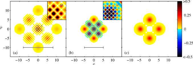
Figure 1: Zurek’s compass state with $a=5/\sqrt{2}$ as depicted by (a) $|\Phi_{\rho}|^{2}$, (b) $(\pi/2)W_{\rho}$, and (c) $\pi Q_{\rho}$. The Wigner function displays fine-scale structure on the scale $\ell_{c}=1/\sqrt{2}a=0.20$, and the size of its large-scale extent is given roughly by $L_{c}=2/\ell_{c}=10$. These scales are reversed in the characteristic function, which has an extent characterized by $\pi/\ell_{c}=\pi L_{c}/2=16$ and fine-scale structure on a scale $\pi/L_{c}=\pi\ell_{c}/2=0.31$. In (a) and (b), the scale bars indicate $\pi L_{c}/2$ and $L_{c}$, respectively, and the insets, which are blow-ups of the regions bounded by dashed lines, show the fine-scale structure in more detail, with scale bars indicating $\pi\ell_{c}/2$ and $\ell_{c}$, respectively.

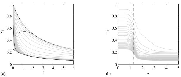
Figure 2: (a) Average fidelity (67) of the compass states for $a=0,0.1,0.2,\dots,5$ (lighter tones from top to bottom) and of the compass state in Fig. 1 (full dark). The upper and lower bounds from Eq. (67) are also shown (dashed), as is the level of fidelity at the critical squeezing parameter $t_{c}=2\ell_{c}^{2}$ (dash-dotted). When $a=0$ the compass state is a single coherent state centered at the origin with fidelity (upper dashed curve) given by Eq. (53). The $a\rightarrow\infty$ bound $1/4(1+t/2)$ from Eq. (67) is shown as the lower dashed curve, most of which is obscured by the full dark line for the state of Fig. 1. The dash-dotted curve shows that to achieve a fidelity of approximately 1/2 or better, we need to teleport with a squeezing parameter $t<t_{c}$. (b) Average fidelity of the compass states as a function of $a$ for $t=0.2,0.4,\dots,6$ (lighter tones from top to bottom). The fidelity declines sharply when $a=\sqrt{\pi/2}$ (dashed), at which point the four coherent states are separated by a distance specified by a von Neumann lattice. This is the separation at which the interference fringes and checkerboard pattern of Fig. 1 appear.

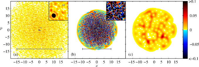
Figure 3: A random state with $N=100$ as depicted by (a) $|\Phi_{\rho}|^{2}$, (b) $(\pi/2)W_{\rho}$, and (c) $\pi Q_{\rho}$. The Wigner function displays fine-scale structure on the scale $\ell_{c}=1/\sqrt{N}=0.10$, and the size of its large-scale extent is given approximately by $L_{c}=2/\ell_{c}=20$. These scales are reversed in the characteristic function, which has an extent characterized by $\pi/\ell_{c}=\pi L_{c}/2=31$ and fine-scale structure on a scale $\pi/L_{c}=\pi\ell_{c}/2=0.16$. The scale bars and insets in (a) and (b) are as in Fig. 1.

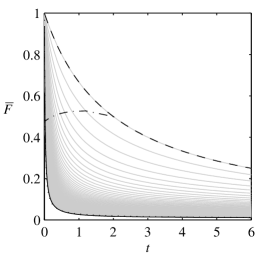
Figure 4: The average fidelity (75) for random states with $N=1,2,\dots,100$ (lighter tones from top to bottom). The case $N=1$, which reduces to the coherent-state fidelity (53), is highlighted (dashed), and the level of fidelity at the critical squeezing value $t_{c}$ is plotted (dash-dotted), showing again that to achieve a fidelity of approximately $1/2$ or better requires $t<t_{c}$. The fidelities of the particular random state in Fig. 4 (dark full) and the chaotic state in Fig. 5 (dotted) are also drawn; they are essentially indistinguishable.

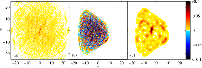
Figure 5: A chaotic state produced by the driven double-well Hamiltonian (79) as depicted by (a) $|\Phi_{\rho}|^{2}$, (b) $(\pi/2)W_{\rho}$, and (c) $\pi Q_{\rho}$.

V.2 Squeezed states

All squeezed states with the same squeezing parameter $u$ have the same average fidelity; so we need only calculate the fidelity for a squeezed vacuum state

$$|0,u\rangle\;\equiv\;e^{u(b^{2}-b^{{\dagger}2})/2}|0\rangle\;.$$ (56)

Using

$$e^{-u(b^{2}-b^{{\dagger}2})/2}D(b,\nu)e^{u(b^{2}-b^{{\dagger}2})/2}\;=\;D(b,\mu\cosh u+\mu^{*}\sinh u)\;=\;D\big{(}b,(e^{u}\mu_{1}+ie^{-u}\mu_{2})/\sqrt{2}\big{)}\;,$$ (57)

we find the characteristic function,

$$\Phi_{|0,u\rangle}(\mu)\;=\;e^{-(e^{2u}\mu_{1}^{2}+e^{-2u}\mu_{2}^{2})/4}\;.$$ (58)

The teleportation fidelity for any squeezed state with squeezing parameter $u$ is then

$$\,\overline{\vphantom{\raisebox{0.34444pt}{F}}F}\!_{|\nu,u\rangle}(t)\;=\;\int\frac{d^{\hskip 0.52498pt2}\mu}{\pi}\,e^{-t|\mu|^{2}/2}e^{-(e^{2u}\mu_{1}^{2}+e^{-2u}\mu_{2}^{2})/2}\;=\;\frac{1}{\sqrt{1+t\cosh 2u+t^{2}/4}}\;,$$ (59)

giving $\ell_{c}=1/\sqrt{\cosh 2u}$ ($L_{c}=2\sqrt{\cosh 2u}$). For a highly squeezed state ($u\gg 1$), we have $\ell_{c}\simeq\sqrt{2}e^{-u}$ and $L_{c}\simeq\sqrt{2}e^{u}$.

V.3 Number states

The number-state matrix elements of the displacement operator are given by Cahill1969

$$\langle m|D(b,\mu)|n\rangle\;=\;\begin{cases}\sqrt{n!/m!}\,e^{-|\mu|^{2}/2}\mu^{m-n}L_{n}^{(m-n)}\bigl{(}|\mu|^{2}\bigr{)}\,,&\;\text{if $m\geq n$}\,,\\ \sqrt{m!/n!}\,e^{-|\mu|^{2}/2}(-\mu^{*})^{n-m}L_{m}^{(n-m)}\bigl{(}|\mu|^{2}\bigr{)}\,,&\;\text{otherwise}\,,\end{cases}$$ (60)

where $L_{n}^{m}(x)$ are generalized Laguerre polynomials Abramowitz . The characteristic function of a number state is a diagonal matrix element:

$$\Phi_{|n\rangle}(\mu)\;=\;\langle n|D(b,\mu)|n\rangle\;=\;e^{-|\mu|^{2}/2}L_{n}\bigl{(}|\mu|^{2}\bigr{)}\;.$$ (61)

The number-state fidelity is thus

$$\,\overline{\vphantom{\raisebox{0.34444pt}{F}}F}\!_{|n\rangle}(t) \;=\;\int\frac{d^{\hskip 0.52498pt2}\mu}{\pi}e^{-(1+t/2)|\mu|^{2}}\big{[}L_{n}\bigl{(}|\mu|^{2}\bigr{)}\big{]}^{2}$$ (62)

$$\;=\;\int_{0}^{\infty}dx\;e^{-(1+t/2)x}\big{[}L_{n}(x)\big{]}^{2}$$ (63)

$$\;=\;\frac{(2n)!}{(n!)^{2}}(1+t/2)^{-2n-1}F\big{(}-n,-n;-2n;1-t^{2}/4\big{)}$$ (64)

$$\;=\;\frac{(1-t/2)^{n}}{(1+t/2)^{n+1}}\,P_{n}\!\left(\frac{1+t^{2}/4}{1-t^{2}/4}\right)\;,$$ (65)

where $F(a,b;c;x)$ is a hypergeometric function, $P_{n}(x)$ is the Legendre polynomial, and we have used formulae found in Refs. Abramowitz ; Gradshtein . Using Eq. (43), we find that $\ell_{c}=1/\sqrt{2n+1}$. More directly, we can use the number-state variances $(\Delta x)^{2}=(\Delta p)^{2}=n+\frac{1}{2}$ to find $2/\ell_{c}=L_{c}=2\sqrt{2n+1}$.

V.4 Zurek’s compass state

Zurek introduced the “compass state” in his original article on sub-Planck structures Zurek2001 . It is a superposition of four coherent states at positions $(x,p)=(\sqrt{2}a,0)$, $(-\sqrt{2}a,0)$, $(0,\sqrt{2}a)$, and $(0,-\sqrt{2}a)$:

$$|\maltese\rangle\;=\;\frac{|a\rangle+|{-}a\rangle+|ia\rangle+|{-}ia\rangle}{2e^{-a^{2}/2}\sqrt{2(\cosh{a^{2}}+\cos{a^{2}})}}\;.$$ (66)

A straightforward, but laborious calculation yields the average teleportation fidelity:

$$\,\overline{\vphantom{\raisebox{0.34444pt}{F}}F}\!_{|\maltese\rangle}(t) \;=\;\frac{1}{4(1+t/2)}\left[1+\frac{\displaystyle{\left(\cosh\frac{2-t}{2+t}a^{2}+\cos\frac{2-t}{2+t}a^{2}\right)^{2}+2\!\left(\cosh a^{2}+\cos\frac{2-t}{2+t}a^{2}\right)\!\!\left(\cos a^{2}+\cosh\frac{2-t}{2+t}a^{2}\right)}}{\displaystyle{\vphantom{\bigg{(}}\left(\cosh a^{2}+\cos a^{2}\right)^{2}}}\right]$$

$$\;\rightarrow\;\begin{cases}\displaystyle{\vphantom{\Bigg{(}}\frac{1}{1+t/2}}\;,&\text{for $a\rightarrow 0$}\,,\\ \displaystyle{\vphantom{\Bigg{(}}\frac{1}{4(1+t/2)}}\;,&\text{for $a\rightarrow\infty$}\,.\end{cases}$$ (67)

Differentiating this expression gives

$$\ell_{c}\;=\;\left(1+2a^{2}\frac{\sinh a^{2}-\sin a^{2}}{\cosh a^{2}+\cos a^{2}}\right)^{-1/2}\;\simeq\;\frac{1}{\sqrt{2}a}\quad\text{for $a\rightarrow\infty$}\;.$$ (68)

More directly, one can evaluate $(\Delta x)^{2}+(\Delta p)^{2}$ and use Eq. (48) to find $\ell_{c}=2/L_{c}$.

The Wigner function of a compass state with $a=5/\sqrt{2}$, which is well into the regime of large $a$, is shown in Fig. 1(b). Interference fringes form between adjacent coherent states, combining at the origin to create a checkerboard of fine structure at a scale on the order of $\ell_{c}=1/\sqrt{2}a=1/5$. Complementary behavior is displayed in the Fourier transform, the characteristic function, whose absolute square is plotted in Fig. 1(a). The Husimi function [Fig. 1(c)] can be viewed as a Gaussian smoothing of the Wigner function. The average teleportation fidelity (67) for a compass state is plotted in Fig. 2(a) for various values of $a$. The caption explains in detail the various features plotted in Fig. 2.

V.5 Random states

We now consider states of the form

$$|\psi\rangle\;=\;\sum_{n=0}^{N-1}c_{n}|n\rangle$$ (69)

where the states $|n\rangle$ are the number eigenstates and the coefficients $c_{n}$ form a a random complex unit vector in $N$ dimensions under the uniform measure, i.e., a random point on the unit sphere in $2N$ dimensions. These states are conjectured to have the same statistical properties as an eigenstate (or long-time evolved state) of a chaotic system with a region of ergodicity within a circle of radius $r=\sqrt{2N}$ in phase space Leboeuf1999 . Figure 3 plots the absolute square of the characteristic function, the Wigner function, and the Husimi function for an example random state with $N=100$.

To calculate the average fidelity of a random state, we use the fidelity in the form (37d), noting that the absolute square of the characteristic function for any state of the form (69) is given by

$$|\Phi_{\rho}(\mu)|^{2}\;=\;\left|\langle\psi|D(b,\mu)|\psi\rangle\right|^{2}\;=\;\sum_{m,n,k,j=0}^{N-1}c_{n}c_{m}^{*}c_{j}c_{k}^{*}\langle m|D(b,\mu)|n\rangle\langle k|D^{\dagger}(b,\mu)|j\rangle\;,$$ (70)

The necessary averages over random states as described above are given by

$$\mathrm{E}\!\left[c_{n}c_{m}^{*}c_{j}c_{k}^{*}\right]\;=\;\frac{\delta_{mn}\delta_{jk}+\delta_{mj}\delta_{nk}}{N(N+1)}\;.$$ (71)

These averages imply that $\mathrm{E}[c_{n}c_{m}^{*}]=\delta_{nm}/N$. As a result, we have

$$\mathrm{E}\!\left[|\Phi_{\rho}(\mu)|^{2}\right]\;=\;\frac{1}{N(N+1)}\sum_{m,n=0}^{N-1}\Big{(}\langle m|D(b,\mu)|m\rangle\langle n|D^{\dagger}(b,\mu)|n\rangle+\langle m|D(b,\mu)|n\rangle\langle n|D^{\dagger}(b,\mu)|m\rangle\Big{)}\;.$$ (72)

Using Eq. (60) and Ref. Gradshtein , one can show that

$$\int\frac{d^{\hskip 0.52498pt2}\mu}{\pi}e^{-t|\mu|^{2}/2}\langle m|D(b,\mu)|n\rangle\langle n|D^{\dagger}(b,\mu)|m\rangle \;=\;\frac{(m+n)!}{m!\,n!\,(1+t/2)^{m+n+1}}F\big{(}-m,-n;-m-n;1-t^{2}/4\big{)}\;,$$ (73)

$$\int\frac{d^{\hskip 0.52498pt2}\mu}{\pi}e^{-t|\mu|^{2}/2}\langle m|D(b,\mu)|m\rangle\langle n|D^{\dagger}(b,\mu)|n\rangle \;=\;\frac{(m+n)!(t/2)^{m+n}}{m!\,n!\,(1+t/2)^{m+n+1}}F\big{(}-m,-n;-m-n;1-4/t^{2}\big{)}\;,$$ (74)

which gives

$$\mathrm{E}\!\left[\,\overline{\vphantom{\raisebox{0.34444pt}{F}}F}\!_{|\psi\rangle}(t)\right]\;=\;\frac{1}{N(N+1)}\sum_{m,n=0}^{N-1}\frac{(m+n)!}{m!\,n!\,(1+t/2)^{m+n+1}}\Big{[}F\big{(}-m,-n;-m-n;1-t^{2}/4\big{)}\\ +(t/2)^{m+n}F\big{(}-m,-n;-m-n;1-4/t^{2}\big{)}\Big{]}\;.$$ (75)

This average fidelity is plotted in Fig. 4 for $N=1,2,\dots,100$ (lighter tones).

To calculate the slope of the fidelity at $t=0$, it is easiest to work from Eq. (48) to obtain

$$-\frac{1}{2}\left[(\Delta x)^{2}+(\Delta p)^{2}\right]\;=\;\left.\frac{d\,\overline{\vphantom{\raisebox{0.34444pt}{F}}F}\!_{|\psi\rangle}}{dt}\right|_{t=0}\;=\;-\frac{1}{2}\sum_{n=0}^{N-1}(2n+1)|c_{n}|^{2}+\sum_{m,n=0}^{N-2}\sqrt{(n+1)(m+1)}c_{n}^{*}c_{n+1}c_{m}c_{m+1}^{*}\;.$$ (76)

Averaging over random states leads to

$$-\frac{1}{2}\mathrm{E}\!\left[(\Delta x)^{2}+(\Delta p)^{2}\right]\;=\;\mathrm{E}\!\left[\left.\frac{d\,\overline{\vphantom{\raisebox{0.34444pt}{F}}F}\!_{|\psi\rangle}}{dt}\right|_{t=0}\right]\;=\;\left.\frac{d\,\mathrm{E}\bigl{[}\,\overline{\vphantom{\raisebox{0.34444pt}{F}}F}\!_{|\psi\rangle}\bigr{]}}{dt}\right|_{t=0}\;=\;-\,\frac{N^{2}+1}{2(N+1)}\;.$$ (77)

We now define our measures of small- and large-scale structure to be

$$2/\ell_{c}\;=\;L_{c}\;=\;2\sqrt{\mathrm{E}\!\left[(\Delta x)^{2}+(\Delta p)^{2}\right]}\;=\;2\sqrt{\frac{N^{2}+1}{N+1}}\;\simeq\;2\sqrt{N}\quad\text{for $N\rightarrow\infty$}\;,$$ (78)

ignoring that the averaging over random states doesn’t commute with taking square roots and reciprocals, although it will do so very closely when $N$ is large.

V.6 Chaotic state

We now consider briefly sub-Planck structure in states of a chaotic Hamiltonian. Consider a long-time evolved state of the driven double-well potential, corresponding to Hamiltonian

$$H\;=\;5p^{2}-8x^{2}+0.05x^{4}+65x\cos(2\pi t)\;.$$ (79)

For the parameters chosen in this Hamiltonian, this system is chaotic in the classical limit. By choosing an initial coherent state centered at $(x,p)=(-8,4)$ and then evolving the system from $t=0$ to $t=5$, we obtain the chaotic state pictured in Fig. 5. The Wigner function displays an abundant fine-scale structure that qualitatively resembles that of the random state depicted in Fig. 3. It is no surprise that the fidelity curve also follows that for random states. This is plotted in Fig. 4 as the dotted curve, but is obscured behind the fidelity for the random state (full dark).

VI Mixed-state teleportation and entanglement fidelity

In the preceding sections the teleported state was assumed to be pure. Since teleportation is a linear operation, the procedure outlined in Sec. III works equally well for mixed states. The overlap between input and output states, however, is no longer an appropriate measure of teleportation fidelity. A suitable measure for assessing the fidelity with which a mixed state $\rho$ is teleported is the entanglement fidelity Schumacher1996 , which is the fidelity for teleporting Victor’s half of a purification of $\rho$, thus transferring the entanglement to Bob (entanglement swapping). It is quite easy to see how to generalize all of our results to entanglement fidelity. Victor’s mode is now entangled with another mode, labeled by $U$, which has annihilation operator $u$ and corresponding complex variable $\mu$. The joint state of $U$ and $V$ is a pure state $\rho_{UV}=|\psi_{UV}\rangle\langle\psi_{UV}|$, which purifies Victor’s state, i.e., ${\rm tr}_{U}(\rho_{UV})=\rho$. The results of Sec. III [Eqs. (17), (19), (21), (24) and (25)] generalize immediately to the following:

$$p(\xi) \;=\;\int d^{\hskip 0.52498pt2}\mu\,d^{\hskip 0.52498pt2}\nu\,W_{\rho_{UV}}(\mu,\nu)W_{\rho_{A}}(\xi^{*}-\nu^{*})\;,$$ (80)

$$W_{\rho_{\rm out}}(\mu,\beta|\,\xi) \;=\;\frac{1}{p(\xi)}\int d^{\hskip 0.52498pt2}\nu\,W_{\rho_{UV}}(\mu,\nu)W_{\rho_{AB}}(\xi^{*}-\nu^{*},\beta-\xi)\;,$$ (81)

$$W_{\overline{\rho}_{\rm out}}(\mu,\beta) \;=\;\int d^{\hskip 0.52498pt2}\nu\,P(\nu)W_{\rho_{UV}}(\mu,\beta-\nu)\;,$$ (82)

$$\overline{\rho\vphantom{\raisebox{0.08612pt}{$\rho$}}}_{\rm out} \;=\;\int d^{\hskip 0.52498pt2}\nu\,P(\nu)\,\left[I\otimes D(b,\nu)\right]\,\rho_{UV}\left[I\otimes D^{\dagger}(b,\nu)\right]\;,$$ (83)

$$\Phi_{\overline{\rho}_{\rm out}}(\nu,\alpha) \;=\;\pi\tilde{P}(\alpha)\Phi_{\rho_{UV}}(\nu,\alpha)\;,$$ (84)

The entanglement fidelity averaged over outcomes $\xi$ is

$$\,\overline{\vphantom{\raisebox{0.34444pt}{F}}F}\!^{\hskip 1.75pt{\rm ent}}_{\rho}\;=\;\langle\psi_{UV}|\,\overline{\rho\vphantom{\raisebox{0.08612pt}{$\rho$}}}_{\rm out}|\psi_{UV}\rangle\;=\;\pi^{2}\int d^{\hskip 0.52498pt2}\mu\,d^{\hskip 0.52498pt2}\beta\,W_{\overline{\rho}_{\rm out}}(\mu,\beta)W_{\rho_{UV}}(\mu,\beta)\;;$$ (85)

notice that when $\rho$ is pure, so that $|\psi_{UV}\rangle$ is a product state, the entanglement fidelity reduces to the ordinary fidelity (27). The average entanglement fidelity can be put in the four forms analogous to Eqs. (28):

$$\,\overline{\vphantom{\raisebox{0.34444pt}{F}}F}\!^{\hskip 1.75pt{\rm ent}}_{\rho} \;=\;\int d^{\hskip 0.52498pt2}\nu\,P(\nu)|\Phi_{\rho}(\nu)|^{2}$$ (86a)

$$\;=\;\pi\!\int d^{\hskip 0.52498pt2}\beta\,d^{\hskip 0.52498pt2}\nu\,\tilde{P}(\beta-\nu)W_{\rho}(\beta)W_{\rho}(\nu)$$ (86b)

$$\;=\;\pi\!\int d^{\hskip 0.52498pt2}\beta\,d^{\hskip 0.52498pt2}\nu\,P(\beta-\nu)\left[\pi\!\int d^{\hskip 0.52498pt2}\mu\,W_{\rho_{UV}}(\mu,\beta)W_{\rho_{UV}}(\mu,\nu)\right]\;,$$ (86c)

$$\;=\;\int d^{\hskip 0.52498pt2}\alpha\,\tilde{P}(\alpha)\left[\int\frac{d^{\hskip 0.52498pt2}\nu}{\pi}\,|\Phi_{\rho_{UV}}(\nu,\alpha)|^{2}\right]\;.$$ (86d)

The first line, Eq. (86a), comes from inserting $\overline{\rho\vphantom{\raisebox{0.08612pt}{$\rho$}}}_{\rm out}$ into the first form of the fidelity in Eq. (85). Fourier transforming the terms in the integrand yields the second line, Eq. (86b). This Fourier pair is identical to the upper two lines in the pure-state teleportation fidelity (28); they relate the entanglement fidelity to the large-scale extent of the Wigner function of $\rho$ or, equivalently, to the fine-scale structure of the characteristic function of $\rho$. The third and fourth lines come from writing the entanglement fidelity as an overlap of joint Wigner functions or joint characteristic functions. These two lines also constitute a Fourier pair, which relates the average entanglement fidelity to the fine-scale structure in the joint Wigner function $W_{\rho_{UV}}(\mu,\beta)$ or, equivalently, to the large-scale extent of the joint characteristic function $\Phi_{\rho_{UV}}(\nu,\alpha)$. This Fourier pair is different from the corresponding third and fourth lines for the pure-state fidelity (28) precisely because these properties appear in the joint functions, not in the Wigner and characteristic functions for $\rho$ alone.

We can, however, convert the third and fourth lines to forms that involve only system operators. For this purpose, we focus first on the characteristic-function integral

$$\int\frac{d^{\hskip 0.52498pt2}\nu}{\pi}\,|\Phi_{\rho_{UV}}(\nu,\alpha)|^{2}\;=\;\int\frac{d^{\hskip 0.52498pt2}\nu}{\pi}\,|\Phi_{\rho_{UV}}(-\nu^{*},\alpha)|^{2}\;.$$ (87)

The reason for the term on the right becomes clear as we manipulate this integral below. Since the entanglement fidelity is independent of which purification is used, we can use the purification

$$|\psi_{UV}\rangle\;=\;\sum_{n=0}^{\infty}|n\rangle_{U}\otimes\sqrt{\rho}\,|n\rangle_{V}\;,$$ (88)

where $|n\rangle_{U}$ and $|n\rangle_{V}$ denote number states for $U$ and $V$, respectively.

The characteristic function now becomes

$$\Phi_{\rho_{UV}}(-\nu^{*},\alpha) \;=\;\langle\psi_{UV}|D(u,-\nu^{*})\otimes D(v,\alpha)|\psi_{UV}\rangle$$

$$\;=\;\sum_{m,n}{}_{U}\langle n|D(u,-\nu^{*})|m\rangle_{U}{}_{V}\langle n|\sqrt{\rho}D(v,\alpha)\sqrt{\rho}\,|m\rangle_{V}$$

$$\;=\;\sum_{m,n}{}_{V}\langle m|D(v,\nu)|n\rangle_{V}\langle n|\sqrt{\rho}D(v,\alpha)\sqrt{\rho}\,|m\rangle_{V}$$

$$\;=\;{\rm tr}\bigl{[}D(v,\nu)\sqrt{\rho}D(v,\alpha)\sqrt{\rho}\,\bigr{]}\;,$$ (89)

where in the third step, we use

$${}_{U}\langle n|D(u,-\nu^{*})|m\rangle_{U}\;=\;{}_{U}\langle n|D(u,-\nu)|m\rangle_{U}^{*}\;=\;{}_{U}\langle m|D(u,\nu)|n\rangle_{U}\;=\;{}_{V}\langle m|D(v,\nu)|n\rangle_{V}\;.$$ (90)

Inserting Eq. (89) into the integral (87) gives us a form that involves only system operators:

$$\int\frac{d^{\hskip 0.52498pt2}\nu}{\pi}\,|\Phi_{\rho_{UV}}(\nu,\alpha)|^{2} \;=\;\int\frac{d^{\hskip 0.52498pt2}\nu}{\pi}\,\Bigl{|}{\rm tr}\bigl{[}D(v,\nu)\sqrt{\rho}D(v,\alpha)\sqrt{\rho}\,\bigr{]}\Bigr{|}^{2}$$

$$\;=\;\int\frac{d^{\hskip 0.52498pt2}\nu}{\pi}\,\sum_{m,n}{}_{V}\langle m|\sqrt{\rho}D(v,\alpha)\sqrt{\rho}D(v,\nu)|m\rangle_{V}\langle n|D^{\dagger}(v,\nu)\sqrt{\rho}D^{\dagger}(v,\alpha)\sqrt{\rho}\,|n\rangle_{V}$$ (91)

$$\;=\;\sum_{n}{}_{V}\langle n|\sqrt{\rho}D(v,\alpha)\sqrt{\rho}\sqrt{\rho}D^{\dagger}(v,\alpha)\sqrt{\rho}\,|n\rangle_{V}$$ (92)

$$\;=\;{\rm tr}\big{[}\rho D^{\dagger}(v,\alpha)\rho D(v,\alpha)\big{]}\;.$$ (93)

The simplification in the third step follows from

$$\int\frac{d^{\hskip 0.52498pt2}\nu}{\pi}\,D(b,\nu)|m\rangle_{V}\langle n|D^{\dagger}(b,\nu)\;=\;\delta_{mn}I\;,$$ (94)

which is a consequence of Schur’s Lemma for the (Weyl-Heisenberg) group of displacement operators, but which can also be derived directly, for example, from Eq. (60).

The joint Wigner-function integral in Eq. (86c) can now be obtained by a Fourier transform of all variables in the characteristic-function integral (93):

$$\pi\!\int d^{\hskip 0.52498pt2}\mu\,W_{\rho_{UV}}(\mu^{*},\beta)W_{\rho_{UV}}(\mu^{*},\nu)\;=\;\frac{1}{\pi^{2}}\,{\rm tr}\bigl{[}\rho\tilde{D}(v,\beta)\rho\tilde{D}(v,\nu)\bigr{]}\;\equiv\;\bm{W}_{\rho}(\beta,\nu)\;.$$ (95)

Here $\tilde{D}(v,\nu)$ is the Fourier transform of the displacement operator, as in Eq. (8), and we define the two-variable function $\bm{W}_{\rho}(\beta,\nu)$. For a pure state $\rho$, $\bm{W}_{\rho}(\beta,\nu)=W_{\rho}(\beta)W_{\rho}(\nu)$, and for mixed states, $\bm{W}_{\rho}(\beta,\nu)$ is what replaces the product of Wigner functions in the third form (28c) of the teleportation fidelity. The Fourier transform of $\bm{W}_{\rho}(\beta,\nu)$ is

$$\bm{\Phi}_{\rho}(\mu,\alpha)\;=\;\int d^{\hskip 0.52498pt2}\beta\,d^{\hskip 0.52498pt2}\nu\,\bm{W}_{\rho}(\beta,\nu)D^{*}(\beta,\mu)D(\nu,\alpha)\;=\;{\rm tr}\big{[}\rho D^{\dagger}(v,\mu)\rho D(v,\alpha)\big{]}\;,$$ (96)

For a pure state $\rho$, we have $\bm{\Phi}_{\rho}(\mu,\alpha)=\Phi_{\rho}^{*}(\mu)\Phi_{\rho}(\alpha)$.

We can now summarize our results by rewriting the third and fourth lines in the entanglement fidelity [Eqs. (86c) and Eqs. (86d)], the lines that tell us about fine-scale phase-space structure, in terms of the new bold-face functions:

$$\,\overline{\vphantom{\raisebox{0.34444pt}{F}}F}\!^{\hskip 1.75pt{\rm ent}}_{\rho} \;=\;\pi\!\int d^{\hskip 0.52498pt2}\beta\,d^{\hskip 0.52498pt2}\nu\,P(\beta-\nu)\bm{W}_{\rho}(\beta,\nu)$$ (97a)

$$\;=\;\int d^{\hskip 0.52498pt2}\mu\,\tilde{P}(\mu)\,\bm{\Phi}_{\rho}(\mu,\mu)\;.$$ (97b)

These forms can be specialized to the case of squeezed-state teleportation by inserting the expressions for $P$ and $\tilde{P}$ from Eqs. (31) and (32).

When we repeat the steps of Sec. IV to find the first derivative of the entanglement fidelity, the sequence of Eq. (48) is unchanged, because it uses the upper Fourier pair in Eq. (86), but the sequence of Eq. (44), which uses the lower Fourier pair, must be modified to use the bold-face functions. The resulting expressions for the derivative,

$$\left.\frac{d\,\overline{\vphantom{\raisebox{0.34444pt}{F}}F}\!^{\hskip 1.75pt{\rm ent}}_{\rho}}{dt}\right|_{t=0}\;=\;-\frac{1}{2}\left({\Delta x_{V}}^{2}+{\Delta p_{V}}^{2}\right)\;=\;-\frac{\pi}{2}\int d^{\hskip 0.52498pt2}\nu\,\left.\frac{\partial^{\hskip 0.70004pt2}\bm{W}_{\rho}(\nu,\alpha)}{\partial\nu^{*}\,\partial\alpha}\right|_{\alpha=\nu}\;,$$ (98)

give rise to the mixed-state generalizations of our measures for small- and large-scale phase space structure:

$$\left(-2\left.\frac{d\,\overline{\vphantom{\raisebox{0.34444pt}{F}}F}\!^{\hskip 1.75pt{\rm ent}}_{\rho}}{dt}\right|_{t=0}\right)^{1/2}\;=\;\frac{1}{\ell_{c}}\;=\;\frac{L_{c}}{2}\;=\;\sqrt{{\Delta x_{V}}^{2}+{\Delta p_{V}}^{2}}\;=\;\left(\pi\int d^{\hskip 0.52498pt2}\nu\,\left.\frac{\partial^{\hskip 0.70004pt2}\bm{W}_{\rho}(\nu,\alpha)}{\partial\nu^{*}\,\partial\alpha}\right|_{\alpha=\nu}\right)^{1/2}\;.$$ (99)

It is instructive to see how this works out for a thermal state,

$$\rho=(1-e^{-\lambda})e^{-\lambda b^{\dagger}b}\;=\;\int\frac{d^{\hskip 0.52498pt2}\beta}{\pi\bar{n}}\,e^{-|\beta|^{2}/\bar{n}}|\beta\rangle\langle\beta|\;,$$ (100)

where $\lambda$ is the dimensionless inverse temperature and $\bar{n}=(e^{\lambda}-1)^{-1}$ is the mean number of quanta. The second form is the standard $P$-function representation of a thermal state Cahill1969 . Inserting the $P$-function representation into the expression (96) gives

$$\bm{\Phi}(\mu,\alpha)\;=\;\frac{1}{2\bar{n}+1}\exp\!\left(-\frac{2\bar{n}^{2}+2\bar{n}+1}{2(2\bar{n}+1)}\bigl{(}|\mu|^{2}+|\alpha|^{2}\bigr{)}+\frac{\bar{n}(\bar{n}+1)}{2\bar{n}+1}(\mu\alpha^{*}+\mu^{*}\alpha)\right)$$ (101)

and thus

$$\bm{\Phi}(\mu,\mu)\;=\;\frac{1}{2\bar{n}+1}e^{-|\mu|^{2}/(2\bar{n}+1)}\;.$$ (102)

The resulting average entanglement fidelity from Eq. (97b) is

$$\,\overline{\vphantom{\raisebox{0.34444pt}{F}}F}\!^{\hskip 1.75pt{\rm ent}}_{\rho}\;=\;\frac{1}{1+(2\bar{n}+1)t/2}\;.$$ (103)

This gives

$$\frac{1}{\ell_{c}}=\frac{L_{c}}{2}=\sqrt{2\bar{n}+1}\;,$$ (104)

which is consistent with the variances of $x$ and $p$, i.e., $(\Delta x)^{2}+(\Delta p)^{2}=2\bar{n}+1$.

VII Conclusion

In this paper we examined the relationships among the output fidelity of continuous-variable teleportation protocols, sub-Planck structure in the Wigner function of the teleported state, and the large-scale extent of that Wigner function. For pure states, these relationships are made mathematically precise in Eqs. (44) and (48), which lead us to define measures of small- and large-scale structure for the Wigner function in Eqs. (47) and (50). Consideration of several example states in Sec. V illuminates these relationships and builds confidence that the measures of small- and large-scale structure we define are quite reliable measures of phase-space properties of the Wigner function.

The generalization of these results to mixed states in Sec. VII leads to a pair of new functions, generalizations of the Wigner and characteristic functions, which capture the fine-scale phase-space structure in any purification of the mixed state. These new functions might prove useful in other studies of phase-space properties of mixed states.

- (1) C. H. Bennett, G. Brassard, C. Crépeau, R. Jozsa, A. Peres, and W. K. Wootters, Phys. Rev. Lett. 70, 1895 (1993).
- (2) L. Vaidman, Phys. Rev. A 49, 1473 (1994).
- (3) S. L. Braunstein and H. J. Kimble, Phys. Rev. Lett. 80, 869 (1998).
- (4) S. L. Braunstein, G. M. D’Ariano, G. J. Milburn, and M. F. Sacchi, Phys. Rev. Lett. 84, 3486 (2000).
- (5) W. K. Wootters and W. H. Zurek, Nature 299, 802 (1982).
- (6) D. Dieks, Phys. Lett. 92A, 271 (1982).
- (7) M. A. Nielsen and I. L. Chuang, Quantum Computation and Quantum Information (Cambridge University Press, Cambridge, 2000).
- (8) A. Furusawa, J. L. Sørensen, S. L. Braunstein, C. A. Fuchs, H. J. Kimble, and E. S. Polzik, Science 282, 706 (1998).
- (9) T. C. Zhang, K. W. Goh, C. W. Chou, P. Lodahl, and H. J. Kimble, Phys. Rev. A 67, 033802 (2003).
- (10) W. P. Bowen, N. Treps, B. C. Buchler, R. Schnabel, T. C. Ralph, H.-A. Bachor, T. Symul, and P. K. Lam, Phys. Rev. A 67, 032302 (2003).
- (11) H. Yonezawa, T. Aoki, and A. Furusawa, Nature 431, 430 (2004).
- (12) N. Takei, H. Yonezawa, T. Aoki, and A. Furusawa, Phys. Rev. Lett. 94, 220502 (2005).
- (13) N. Takei, T. Aoki, S. Koike, K. Yoshino, K. Wakui, H. Yonezawa, T. Hiraoka, J. Mizuno, M. Takeoka, M. Ban, and A. Furasawa, Phys. Rev. A 72, 042304 (2005).
- (14) H. Yonezawa, S. L. Braunstein, and A. Furusawa, Phys. Rev. Lett. 99, 110503 (2007).
- (15) C. M. Caves and K. Wódkiewicz, Phys. Rev. Lett. 93, 040506 (2004).
- (16) W. H. Zurek, Nature 412, 712 (2001).
- (17) W. J. Munro, K. Nemoto, G. J. Milburn, and S. L. Braunstein, Phys. Rev. A 66, 023819 (2002).
- (18) F. Toscano, D. A. R. Dalvit, L. Davidovich, and W. H.Zurek, Phys. Rev. A 73, 023803 (2006).
- (19) D. A. R. Dalvit, R. L. de Matos Filho, and F. Toscano, New J. Phys. 8, 276 (2006).
- (20) L. Praxmeyer, P. Wasylczyk, C. Radzewicz, K. Wódkiewicz, Phys. Rev. Lett. 98, 063901 (2007).
- (21) A. Ourjoumtsev, R. Tualle-Brouri, J. Laurat, and P. Grangier, Science 312, 83 (2006).
- (22) A. Ourjoumtsev, H. Jeong, R. Tualle-Brouri, and P. Grangier, Nature 448, 784 (2007).
- (23) B. Schumacher, Phys. Rev. A 54, 2614 (1996).
- (24) For a comprehensive, but telegraphic list of properties and relations based on these conventions, see C. M. Caves, “Operator formalism and quasidistributions for creation and annihilation operators,” http://info.phys.unm.edu/~caves/reports/reports.html.
- (25) K. E. Cahill and R. J. Glauber, Phys. Rev. 177, 1857 (1969).
- (26) M. Abramowitz and I. A. Stegun, Handbook of Mathematical Functions (Dover, New York, 1965).
- (27) I. S. Gradshtein and I. M. Ryzhik, Table of integrals, series, and products (Academic, New York, 1980).
- (28) P. Leboeuf, J. Stat. Phys. 95, 651 (1999).