The Central Region of M83

Abstract

We combine VLT/ISAAC NIR spectroscopy with archival HST/WFPC2 and HST/NICMOS imaging to study the central 20″$\times$20″ of M83. Our NIR indices for clusters in the circumnuclear star-burst region are inconsistent with simple instantaneous burst models. However, models of a single burst dispersed over a duration of 6 Myrs fit the data well and provide the clearest evidence yet of an age gradient along the star forming arc, with the youngest clusters nearest the north-east dust lane. The long slit kinematics show no evidence to support previous claims of a second hidden mass concentration, although we do observe changes in molecular gas velocity consistent with the presence of a shock at the edge of the dust lane.

1 Introduction

M83 (NGC 5236) is a nearby (4.5 Mpc; Thim et al. 2003) grand design spiral galaxy SAB(s)c (de Vaucouleurs et al., 1991) in a group containing several bright galaxies including Centaurus A (NGC 5128) and NGC 4945. Within the central 20″ lies the photometric peak (hereafter referred to as the nucleus) offset from the centre of symmetry of the outer bulge isophotes and the global gas kinematics (Wolstencroft, 1988; Gallais et al., 1991; Thatte et al., 2000; Sakamoto et al., 2004) and surrounded by a semicircular starburst region, some 3″ - 8″ from the nucleus. M83 has a close dynamical companion, NGC 5253 (Rogstad et al., 1974) which also contains recent star formation, albeit much more compact than that of M83. The closest passage of NGC 5253 occurred 1-2 Gyrs ago (Rogstad et al., 1974) and so the activity in these galaxies is likely driven by internal inflow of gas via the bar rather than from direct interaction as the clusters are mostly 1-10 Myrs in age (Harris et al., 2001, hereafter H01).

1.1 Central star formation

Gallais et al. (1991) first presented NIR images of sub-arcsecond resolution for the central region of M83 which lead to an improved understanding of the morphology: the region of young stars is composed of a bright circum-nuclear arc of star clusters, located $\sim$7″ from the old nucleus. However, Gallais et al. also attempted to date the young clusters and (contrary to more recent work, discussed later) suggested that the clusters were younger on the south-east end of the arc and older on the north-west end (but with one anomalous young cluster at this old end). They were not alone in this conclusion: Heap et al. (1993), using WFPC photometry and IUE UV spectroscopy also suggested that the age gradient went from south-east to north-west, the youngest clusters being in the south-east end of the arc. Heap et al. also identified that the old stellar nucleus was not a site of H$\alpha$ emission. Puxley et al. (1997) performed low resolution NIR spectroscopy along a single slit bisecting the starburst arc and found evidence for a radial age gradient. Elmegreen et al. (1998) found a double ring structure in their (J-K) colour images of the centre of M83 and associated each ring with an inner Lindblad resonances (ILR).

However, when H01 made a comprehensive study of the star clusters using HST/WFPC2 narrow- and broadband data coupled with the latest Starburst99 population synthesis models (Leitherer et al., 1999, hereafter SB99), they identified that the tangential age gradient along the starburst arc was in fact from north-west to south-east with the youngest clusters in the north-west (in direct conflict with earlier work but resolving the anomalous cluster in Gallais et al. 1991). H01 also found the majority of the clusters in the arc to have ages in the range 5-7 Myrs and found evidence of age gradients perpendicular to the starburst arc with younger clusters along the periphery; they concluded such gradients were indicative of an inside-out propagation of star formation. Subsequently, Bresolin & Kennicutt (2002) found Wolf-Rayet features in UV spectra of clusters near the north-west end of the arc and dated this star formation at 5 Myrs (and the other regions at 7 Myrs), in rough agreement with the estimates in H01 for the similar regions.

1.2 Nuclear Rings

Considering the evidence thus far presented, one would most likely conclude that the circumnuclear arc seen at the centre of M83 is a nuclear ring. Nuclear rings are often found at the centres of barred spiral galaxies (Buta, 1986) as are nuclear spirals (Martini & Pogge, 1999; Pogge & Martini, 2002) and their formation is thought to be very similar. Athanassoula (1992) first showed how the orbits in barred galactic potentials lead to gas shocking on the leading edges to form dust lanes with the shocked gas then flowing along the potential to the centre. These shocks have been observed across dust lanes, both directly as velocity jumps in gas kinematics and indirectly from increased radio emission (both discussed in detail by Athanassoula, 1992).

However, Athanassoula’s early simulations didn’t have the resolution to properly probe the central regions to determine exactly what happened to the inflowing gas; this was done by Piner et al. (1995) using the similar models to Athanassoula but with cylindrical coordinates for better spatial resolution at the centre. Piner et al. found that if the barred potential permitted two ILRs, the gas flow builds up between them to form a dense nuclear ring. This was also confirmed by Combes (1996) and Buta & Combes (1996) who went further to say that even in a potential that admits one ILR, the inflowing gas will build up there to form a ring. Given the rings and ILRs found by Elmegreen et al., it appeared likely that the arc of young stars in M83 was formed from gas building up in this way and leading to star formation.

This ILR picture of nuclear ring formation has persisted despite recent work suggesting subtle differences. Regan & Teuben (2003) performed an exhaustive number of simulations like those of Piner et al. for various barred potentials and they conclude that it is not the presence of ILRs that dictate the formation of a nuclear ring, but the existence and properties of an orbit family, namely the $x_{2}$ family: if this orbit family exists, so can a nuclear ring and the authors find an excellent correlation between the $x_{2}$ orbit of largest extent along the bar major axis and the radius of the nuclear ring. If the $x_{2}$ family does not exist, the authors never find a nuclear ring. There is some discussion as to definitions: an ILR is normally defined as the locus at which the pattern frequency of the bar equals the circular orbital frequency less half the epicyclic orbital frequency, e.g. $\Omega_{b}=\Omega-\kappa/2$, and in weak bars this same definition traces the largest extent of the $x_{2}$ orbit family. However, as Regan & Teuben are careful to point out, in strong bars with a large quadrupole moment and low central mass concentrations, this is no longer the case and there can be regions where $\Omega_{b}<\Omega-\kappa/2$ but no $x_{2}$ orbits exist. Maciejewski (2004) has also performed high resolution hydrodynamical simulations of the central regions of barred galaxies and shows how nuclear rings and nuclear spirals are formed by the same hydrodynamical processes. Although Maciejewski continues the old trend in matching ILRs with the nuclear spiral and ring phenomenon, he is careful to define the ILR as the largest extent of the $x_{2}$ orbit family, implying that the $x_{2}$ family exists when referring to an ILR. We will return to the results in Regan & Teuben (2003) and Maciejewski (2004), particularly to their predictions of the phase space distribution of the gas (velocity and density) in the ring and to the trajectories of stars on $x_{2}$ orbits, formed in the ring.

1.3 Nuclear Disks

There is clearly overwhelming evidence that gas can accumulate in the central regions of barred potentials, although the present high resolution hydrodynamical simulations do not predict if and how the gas may give rise to star formation or how the outflows from the young stars and supernovae would affect the gas flow on the ring. Lower resolution N-body simulations including stars, gas and star formation and then combined hydrodynamical and N-body simulations with star formation were performed by Wozniak et al. (2003) and Wozniak & Champavert (2006) after Emsellem et al. (2001) observed drops in the velocity dispersion at the centres of double-barred spirals (also seen in barred spirals by Chung & Bureau 2004) and couldn’t reproduce them in simple dynamical models. The simulations with gas flows, stellar motions and star formation showed that when gas shocks in a barred potential and flows to the centre, it can produce a central disk. This disk of cold gas then produces young stars which dominate the luminosity of the central region and give rise to a very low velocity dispersion because of the low random motion of the stars in the disk. An important difference between these simulations and the pure hydrodynamical ones discussed earlier is that the gas builds up in a disk and not a ring or spiral; subsequent star formation is similarly distributed in a disk and not a ring. Whether this difference is a resolution problem or something more subtle remains to be seen, although if the surface density of the gas was higher in the central region of the disk, one would expect star formation to initiate there and propagate outwards, potentially leaving an outer ring of young stars as in Kenney et al. (1993) and a radial age gradient in the starformation (consistent with the observations of M83 made by Puxley et al., although H01 report younger star clusters around the periphery of the arc, both on the inner and outer edges).

1.4 Polar rings and disks

However, there are certain complications with the circumnuclear ring interpretation for the centre of M83. Most previous studies discuss an arc of young stars, not a complete ring, apart from Gallais et al. (1991) who claim to observe a complete ring or ellipse of star clusters from their sub-arcsecond H-band image, and Elmegreen et al. (1998) who found circum-nuclear rings in their (J-K) NIR images. The fact that complete ring structures are seen in the NIR and not in the optical is highly suggestive of an obscuration of the complete ring by dust; an idea supported by extinction estimates we present later in §5. And there may be a simple explanation for the obscuration of one half of a ring and not the other: Sofue & Wakamatsu (1994) argue that the north-east dust lane is observed to warp out of the plane of the main disk as it approaches the nucleus and they go so far as to call it polar; a similar warp of the south-west dust lane on the other side of the galaxy might explain why it is also not visible. The hydrodynamical simulations of Athanassoula (1992); Piner et al. (1995); Regan & Teuben (2003); Maciejewski (2004) are all in 2D and are unable to permit such warping out of the disk plane. We therefore have no theoretical predictions of gas inflow producing warped disks, spirals and rings, although we can see similar behaviour in other galaxies such as NGC 5383 (as noted in Sandage & Bedke, 1994). If similar hydrodynamical processes occur in 3D as they do in 2D but the gas inflow can build up in a polar or inclined ring out of the plain of the galactic disk, we would certainly expect the star formation to do likewise and given a highly obscuring and dusty galactic disk, for the inclination of M83 to our line-of-sight we would only see the near side of the inner warped disk and an incomplete ring of young stars, as explained by Sofue & Wakamatsu. However, Sofue & Wakamatsu never comment on the plausibility of the galaxy’s inclination giving rise to the obscuration of the dark south-west dust lane by the luminous bulge.

1.5 Interloping hidden mass concentrations

After studying the centre of M83 with near infra-red (NIR) long-slit kinematics, Thatte et al. (2000, hereafter T00) initially suggested the possibility of a second nucleus or mass concentration after the stellar kinematics across the principal nucleus (Slit E in Fig. 3, cutting the arc of young stars and the ‘bridge’ identified in Gallais et al. 1991) revealed two peaks in the velocity dispersion — one associated with the nucleus and another which was 2$\aas@@fstack{\prime\prime}$7 SW of the nucleus. Assuming that the stars are dynamically relaxed in the gravitational potential, the secondary peak in the dispersion is best explained by invoking the presence of a second dynamically hot but obscured mass concentration (T00). Subsequently, Mast et al. (2006) performed optical integral field spectroscopy (IFS) on the central region and linked a strong velocity gradient in the H$\alpha$ velocity map (3$\aas@@fstack{\prime\prime}$9$\pm$0$\aas@@fstack{\prime\prime}$5 W of the nucleus) to the location of the proposed second obscured mass concentration. However, the same authors (Diaz et al., 2006a, hereafter D06) then performed IFS on a coincident but larger region, with better spatial resolution and in the near infrared (NIR). They then found that the largest gradient in the Pa$\beta$ velocity field was in fact some 7″ WNW of the nucleus and so adopted this position as a likely location for a mass concentration (Díaz et al., 2006b, hereafter D06b). The most recent work (Diaz et al., 2007) now reports three mass concentrations: the visible nucleus and a further two hidden mass concentrations at two different locations, both apparently more massive than the visible nucleus. Despite the inconsistency between H$\alpha$ and Pa$\beta$ kinematics (c.f. Fig. 5 of Mast et al. and Fig. 3 of D06a), gas kinematics in general are well known to exhibit non-gravitational effects (Kormendy & Richstone, 1995) and the strong velocity gradients observed in the gas kinematics could be caused by hydrodynamical effects (e.g. outflows, shocks and spiral density waves) rather than mass concentrations.

Nevertheless, the scenario of D06(a,b) is appealing, given the theory of dynamical friction in a gaseous medium as presented by Ostriker (1999) and the numerical implementation. Simulations of merging black holes (BHs) in a gaseous medium (e.g. Escala et al., 2004; Kim & Kim, 2007) reproduce density wakes tantalisingly similar to the density distributions of the aforementioned nuclear spirals and rings; one would be hard pressed to distinguish between Fig. 5 of Escala et al. (2004) and Fig. 6 of Maciejewski (2004). Furthermore, Fig. 2 in Escala et al. (2004) bears a remarkable resemblance to the scenario seen at the centre of M83, assuming that the high density gaseous wake can initiate star formation. As pointed out by D06(a,b), invoking this scenario nicely explains the age gradient of H01 (and the average age gradient of the H01 data presented in D06b) as well as the off-centred old nucleus.

However, some important queries remain unanswered. If the gradient in the gas kinematics is caused by the gravitational potential, one should see the same effect in the stellar kinematics which are mostly unaffected by shocks or outflows and accurately trace the gravitational potential (although if the shock and accumulation of gas is significant, it may begin to dominate over the smooth potential of the disk and bulge). H01 also date some of the youngest clusters in the arc to be beyond the present location of the interloping mass of D06(a,b). If they are related to the arc of young stars, it is not clear how they got to be there: the high density wake created by the interloping masses in Escala et al. (2004) and Kim & Kim (2007), which we assume leads to star formation and an age gradient, is always trailing and never preceding the interloping mass. Furthermore, the clusters nearest the supposed location of the interloper have been dated at 5 Myrs (H01 and Bresolin & Kennicutt 2002); this is larger than one would expect given the age gradient, the dynamical timescale and their small distance from the interloper (disscussed again in §6).

Perhaps more importantly, there is very little evidence of any merger event having occurred recently (the last 50 Myrs) in M83. The most prominent tidal tail of M83 was first published by Malin & Hadley (1997): it is roughly 27′ in length according to this exposure, subtends around 60^∘ in the north by north-west and is estimated to be between 15′ (20kpc) and 20′ (26kpc) from the centre of M83. Clearly, such an arc is well outside the main galatic disk, defined either as the extent of the HII emission or the Holmberg radius (5$\aas@@fstack{\prime}$1 and 7$\aas@@fstack{\prime}$3 respectively, in Thilker et al., 2005). However, this tidal tail is within the HI distribution as seen in Park et al. (2001) and Miller & Bregman (2005); in fact, both these HI studies see a north-western arc of HI emission. The figures in Park et al. (2001) clearly show this HI arc to extend right over from the north-west to the north-east and they estimate a radius of 25′ from the centre of M83. This is approximately the same location as the stellar arc found by Malin & Hadley (1997) and rescaling and overlaying the two images reveals that they are indeed co-spatial near the north-west tip of the stellar arc but diverge to the north-east with the HI at a larger radius than the stellar feature. Such features are so far outside the main stellar disk of M83 that the disrupted source is unlikely to have fallen via dynamical friction to the bottom of the potential, but is more likely to contribute to the outer halo. In fact, on visualising the aforementioned overlay, one is tempted to assign the disturbed outer HI structure seen in Park et al. (2001) to the capture of a satellite which we now see as the Malin & Hadley stellar arc. Moving closer to the galactic disk, Thilker et al. (2005) report GAIA observations of two bisymmetric filaments or arms just outside the main HII disk (5$\aas@@fstack{\prime}$1), one extending roughly north from the east of the disk and the other extending roughly south from the west of the disk, both approximately 15′ in length. Such beautyfully symmetric filaments of star formation are unlikely to be induced by a merger event, but rather by the remaining HI envelope as the authors propose. The main stellar disk of M83 is remarkably regular (as seen in Fig. 1) with only one potential blemish (see §8): radio studies by Cowan et al. (1994) and Maddox et al. (2006) identify a linear sequence of 3 sources to the north-east of the central region. However, in Maddox et al. (2006), the central source of the three is identified to be coincident with one of the x-ray sources of Soria & Wu (2003) and the authors conclude that this linear structure is a background radio galaxy with two lobes of emission from jets and a central galaxy source..

Finally, the CO map of Sakamoto et al. (2004) is regular and symmetric both in its density and its velocity, which is unlikely to be the case if a recent merger had disturbed the gas sufficiently to ignite star formation in its wake.

1.6 This Study

In this paper we report on the results of combining HST photometry and ESO VLT NIR long-slit spectroscopy at the centre of M83. We address the claims of T00 and D06(a,b) regarding the presence of a second obscured mass concentration by looking for further dynamical signatures in the stellar kinematics at the same locations. In particular, to help identify a cause for the gradient in the gas kinematics seen in D06a, we observe the NIR stellar kinematics at the same location. We also build on the study of H01 and compare optical and NIR indices of clusters in the circumnuclear arc (some of which were undetected in H01) with models for the stellar populations. Although H01 showed that an age gradient existed along the arc from north-west to south-east with the youngest clusters in the north-west, the reddening vector in this study parallels the tracks in the two-colour diagram for ages of 5-10 Myrs, complicating the age analysis (Ryder et al., 2005), particularly because the extinction estimates were derived from the H$\beta$:H$\alpha$ decrement which suffers from low H$\beta$ flux, poor penetration and a small wavelength range. NIR indices can probe deeper into potentially obscured clusters, giving a more representative measure of the ages. Furthermore, clusters can be heavily extincted and therefore overlooked in the visible, which is particularly relevant for very young clusters ($<$ 5 Myrs) which may be dustier and only have a weak intrinsic stellar continuum (Ryder et al., 2005); this is less of a problem in the NIR, but we also present and correct our data using an extinction map derived from the H$\alpha$:Pa$\alpha$ decrement, benefitting from more flux, a larger wavelength range and the penetrating Pa$\alpha$ data.

The structure of this paper is as follows: §2 describes the reduction and homogenisation of data from different instruments; §3 describes the analysis of the data; we briefly discuss some important details regarding the error analysis in §4; §5 presents the results which are subsequently discussed in §6 while §7 concludes.

2 Observations and Data Reduction

We present unpublished VLT/ISAAC data and archival HST/NICMOS and HST/WFPC2 data. The observations and data reduction for each instrument are discussed separately below, followed by details of how they were homogenised. Fig. 3 illustrates the slit positions relative to the HST data.

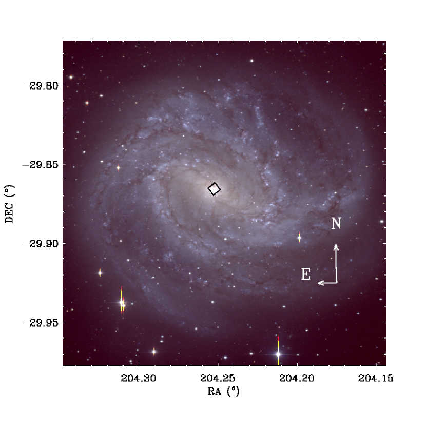
Figure 1: A BVR false-colour image of the spiral galaxy M83 (using logarithmic intensity scaling), with the footprint of the homogenised HST/WFPC2 and HST/NICMOS images overlaid in black. The images were observed using the ESO Danish 1.54m telescope (Larsen & Richtler, 1999)

2.1 VLT/ISAAC Spectroscopy

New K band long-slit spectroscopy along 4 different positions (A, B, C and D in Fig. 3) was observed in late 2000 and we combine this with the original major axis data of T00 (E in Fig. 3) to give a total of 5 slit positions in the central region of M83 observed with the VLT/ISAAC spectrograph using the 0$\aas@@fstack{\prime\prime}$6 slit (0$\aas@@fstack{\prime\prime}$147 pix^-1 plate scale) and an SK filter to give a wavelength range of 2.239µm - 2.362µm at a resolution $(\lambda/\Delta\lambda)$ of 4400. Observations were made using the ABBA technique, removing the need for separate sky exposures. Table 1 summarises other details regarding the exposures.

Date	ID	PA (∘)	Time	DIMM	Data
D/M/Y			(mins)	FWHM	FWHM
11/07/00	[A]	126.95	40 (5)	1$\aas@@fstack{\prime\prime}$02	0$\aas@@fstack{\prime\prime}$6
13/07/00	[A]	126.95	40 (5)	0$\aas@@fstack{\prime\prime}$52	0$\aas@@fstack{\prime\prime}$4
17/08/00	[B]	124.89	30 (5)	0$\aas@@fstack{\prime\prime}$74	0$\aas@@fstack{\prime\prime}$5
18/08/00	[C]	118.13	30 (5)	0$\aas@@fstack{\prime\prime}$61	0$\aas@@fstack{\prime\prime}$5
19/08/00	[D]	171.26	30 (5)	2$\aas@@fstack{\prime\prime}$22	1$\aas@@fstack{\prime\prime}$2
21/03/00	[E]	51.15	15 (5)	0$\aas@@fstack{\prime\prime}$71	0$\aas@@fstack{\prime\prime}$4

Table 1: A summary of the VLT/ISAAC K-band long-slit spectroscopy. The time column gives the total exposure time of all frames and, in parenthesis, the exposure of the individual frames. The last two columns compare the mean seeing reported by the DIMM and the seeing estimated directly from the data (§2.5). The ESO program IDs for the March, July and August exposures are 64.N-0100(B), 265.B-5723(A) and 65.O-0612(A), respectively.

A number of kinematic templates were observed with the same instrumental setup on previous programmes (ESO 64.N-0100 and 65.N-0577). However, this template library lacked supergiants which are typical of a starburst population. Consequently, we supplemented the library with a number of supergiant observations also made with ISAAC but using the 0$\aas@@fstack{\prime\prime}$3 slit (ESO 68.B-0530, 67.B-0504). To homogenise the library, the latter (of higher spectroscopic resolution) were convolved down to match the resolution of the 0$\aas@@fstack{\prime\prime}$6 slit templates. The 0$\aas@@fstack{\prime\prime}$3 slit templates also had a shifted wavelength range (2.249µm- 2.373µm), so both the 0$\aas@@fstack{\prime\prime}$3 and 0$\aas@@fstack{\prime\prime}$6 slit templates were cropped to the common wavelength range. Our final library consisted of 6 giants (K1–M6) and 14 supergiants (K5–M5).

Reduction of the long slit data mainly followed the standard technique, as detailed in the VLT/ISAAC user-manual with use of IRAF and ECLIPSE routines. Minor differences to the above are summarised below.

The raw data frames were corrected for the odd-even effect prior to any other processing using the ECLIPSE Jitter routine. Persistent bad pixels were detected in the flat field images and interpolated over during flat fielding. Subsequently, median filtering was used to detect (but not replace) cosmic rays to make a mask for each data frame. After rectification of the data to a uniform wavelength and spatial grid, the frames were aligned and stacked by fitting a Gaussian to a star cluster in the flux profile of each frame. Crucially, the previous masks were also rectified and shifted in the same manner to identify contamination into neighbouring pixels. All contaminated pixels were then excluded when combining the stacked data frames. Additionally, the data underwent an iterative clipping (at $5\sigma$) as a precaution to eliminate unidentified bad/hot pixels. It is possible to simply remove cosmic rays prior to rectification and alignment by interpolation of neighbouring pixels, but the method employed here interpolates from additional realisations of the same pixel, which we prefer wherever possible.

Telluric standard stars (HD119013 and HD118187) were also observed each night with the same spectrograph setup to correct the other observations for atmospheric absorption, using standard correction techniques (Origlia et al., 1993).

We found that the absolute wavelength calibration of the observations varied each night and was not corrected for by the ARC exposures. To obtain an accurate calibration (the importance of which is described in §2.3), we used the OH emission line at $\lambda_{\textrm{vac}}22460.264\textrm{\AA}$ in the unsubtracted frames as a reference point and corrected accordingly. We further applied a heliocentric velocity correction for each night to correct to an absolute velocity scale.

Slit A was observed over two nights (Table 1) but the seeing varied significantly between them. For all subsequent analysis, we chose to use the data with the best seeing (that of 13/07/00); the increase in the signal-to-noise ratio (SNR) from adding an additional night was marginal and significantly degraded the spatial resolution (increasing cluster contamination). Problems with the arc lamp observations (only the Argon lamp and not the Neon lamp was operating) meant the wavelength calibration was also not as accurate for the 11/07/00 observations of slit A, further motivating our decision to neglect them. The position of slit B, although very similar to that of A, covers a slightly different region and is better centred on a few knots, as can be seen in Fig. 3. We therefore do not combine the data with Slit A, but analyse it separately.

2.2 HST/NICMOS Images

Date	Filter		Time	Mean $\lambda$	Bandpass
D/M/Y			(s)	(Å)	(Å)
WFPC2 (Proposal ID: 8234, PI: Calzetti)
25/04/2000	F300W	(U)	700	3014	858.3
02/05/2000	F487N	(H$\beta$)	1100	4866	33.9
25/04/2000	F547M	(V)	310	5488	637.9
02/05/2000	F656N	(H$\alpha$)	600	6564	28.3
25/04/2000	F814W	(I)	237	8023	1472.8
NICMOS (Proposal ID: 7218, PI: Rieke)
16/05/1998	F187N	(Pa$\alpha$)	160	18740	194.8
16/05/1998	F190N	(cont.)	160	19003	184.0
16/05/1998	F222M	(K)	176	22181	1479.4

Table 2: A summary of the HST observations. Mean wavelengths and bandpasses are calculated with bandpar in the STSDAS synphot package (AVGWV and RECTW, respectively).

The central $20\arcsec\times 20\arcsec$ of M83 were observed with HST/NICMOS in the narrow band filters F187N (Pa$\alpha$), F190N (Pa$\alpha$ continuum) and F222M (approximately K-band), the details of which are shown in Table 2. Fig. 1 illustrates the NICMOS footprint on a false-colour composite (Larsen & Richtler, 1999, observed with the ESO Danish 1.54m telescope and available on NED). All exposures were made with the NICMOS 2 camera with an approximate plate scale of 0$\aas@@fstack{\prime\prime}$075 per pixel (see §2.4). The data were reduced using the STSCI calibration pipeline. However, for exposures observed in non-chopping mode (i.e. without background exposures), the latter stage of the pipeline (calnicb) assumes a sparsely populated field and is configured to estimate and subtract off the background level from the same exposure. It does this by identifying and masking sources (groups of 2 or more pixels $4.5\sigma$ higher than the image median) and using the remaining sigma clipped median as the background level. It is not difficult to see that for our non-chopped observations of the centre of M83, this process will lead to gross over subtraction of the background. Consequently, the value estimated for the background by the pipeline is added back onto the images. They are then flux calibrated using the photometric zero-point PHOTFLAM calculated by the STSCI pipeline and RECTW bandpasses (for narrow-band images) from the STSDAS bandpar routine. The background of each mosaiced exposure is estimated from a suitable blank region near the edge of the frame which is then subtracted.

2.3 HST/WFPC2 Images

$V_{\textrm{rec}}$	H$\alpha$ Trans.	${\rm[NII]\over H{\alpha}}$	H$\beta$ Trans.	${\rm F656N\over F487N}$
(km s-1)	Ratio (%)		Ratio (%)
500	82.6	24.6	96.8	0.83
512	80.6	25.2	96.5	1.03
550	72.8	27.9	95.8	1.12
600	59.5	34.0	94.8	1.32

Table 3: The effect of [NII] contamination and filter transmission with recession velocity $V_{\textrm{rec}}$ for a Gaussian H$\alpha$ emission line of 150km s^-1 FWHM. The columns represent: the recession velocity of the gas $V_{\textrm{rec}}$; the H$\alpha$ transmission at $V_{\textrm{rec}}$ as a percentage of the transmission at $V_{\textrm{rec}}=0$km s^-1; the [NII] contamination as a percentage of the H$\alpha$ emission; the H$\beta$ transmission at $V_{\textrm{rec}}$ as a percentage of the transmission at $V_{\textrm{rec}}=0$km s^-1; the ratio of the observed (uncorrected) fluxes in the F656N (H$\alpha$) filter and the F487N (H$\beta$) filters with $V_{\textrm{rec}}$ (note the effect this may have on extinction estimates using these filters).

The central $36\arcsec\times 36\arcsec$ of M83 was observed with WFPC2 in the filters F814W, F547M, F300W, F487N (H$\beta$) and F656N (H$\alpha$), details of which are given in Table 2.

The data were reduced using the STSCI calibration pipeline. In addition, the STSDAS routine wfixup was used to interpolate over known bad pixels. Flux calibration was performed using the PHOTFLAM photometric zero point calculated by the STSCI pipeline and RECTW bandpasses (for narrow-band images) from the STSDAS bandpar routine.

The transmission curves of the F656N and F814W filters were obtained from the STSDAS calcband routine. Using the optical spectra of Storchi-Bergmann et al. (1995), the [NII] and H$\alpha$ emission lines were fitted (with Gaussians) and subtracted; subsequently applying the F656N and F814W filter curves gave the ratio of the continuum flux in each of the filters. Background subtraction for the F656N image was then performed using the F814W image multiplied by this normalisation factor (as done by H01).

There are two systematic errors associated with the background subtracted F656N observations which required correction. Firstly, the F656N filter is broad enough to include [NII] emission in addition to the H$\alpha$ emission. Secondly, because of the recession velocity of M83, H$\alpha$ lies near the edge of the bandpass, reducing the observed H$\alpha$. These two systematic errors are also correlated: the recession velocity of M83 shifts the $\lambda_{\textrm{vac}}6585.27\textrm{\AA}$ [NII] line out of the bandpass, significantly reducing the contribution from this line. However, it also shifts the $\lambda_{\textrm{vac}}6549.86\textrm{\AA}$ [NII] line into the bandpass, increasing the contribution.

Correcting for these two effects is not trivial. Using the optical spectra of Storchi-Bergmann et al. (1995), one may attempt to correct for both, but the spectra are low resolution (FWHM $\sim$ 10Å $\sim$ 500km s^-1) causing the lines to be significantly broadened. Such instrumental broadening hinders our calculations as it is not possible to reliably estimate the change in transmission for a recession velocity of 500km s^-1 when the line itself is 500km s^-1 in width. Therefore we fit the H$\alpha$ and [NII] lines in the Storchi-Bergmann et al. (1995) spectra with Gaussians to estimate their relative fluxes and then reproduce the spectrum with lines in the same flux ratios but each with a FWHM=150km s^-1 (in agreement with the ionised gas kinematics of D06). Using this (continuum subtracted) spectrum, we calculate the contribution of the [NII] lines and the transmission of the H$\alpha$ line in the F656N image for a range of recession velocities. Table 3 summarises our findings.

Although D06 quote absolute ionised gas velocities ranging between 550km s^-1 and 650km s^-1, the stellar velocity field is not given, so we have no knowledge of whether the ionised gas is actually at a different velocity to the stars or if the absolute wavelength scale is in conflict with the recent determination of $V_{rec}=512$km s^-1by Koribalski et al. (2004). This latter value is in good agreement with the average recession velocity found in the HyperLEDA database (507km s^-1). We took considerable pains to calibrate our ISAAC data to an absolute heliocentric velocity scale (§2.1). The error weighted mean stellar velocity along all slits was found to be 520km s^-1. However, the error weighted mean molecular Hydrogen velocity was found to be 512km s^-1. We therefore adopt the value of Koribalski et al. (2004) for the ionised gas and correct accordingly. Quite by chance, the [NII] contamination and bandpass edge effects almost counteract each other at this velocity, leaving only an overall scaling of 0.99 for the F656N image.

The spectra of Storchi-Bergmann et al. (1995) are averages over the central region and although we attempt to account for the non-uniform gas velocity across the FoV with a systematic error (see §4.3), we might also expect variations in the [NII]:H$\alpha$ flux ratio. Thus our correction in this matter is only to first order.

The effect of recession velocity is smaller for the WFPC2 F487N (H$\beta$) filter (Table 3) and is non-existent for the NICMOS F187N (Pa$\alpha$) filter so the F487N image received a minor flux correction of 1.036 in accordance with Table 3 (neither filter is contaminated by other emission lines).

2.4 Merging HST/WFPC2 data with HST/NICMOS data

HST narrow band images exist in H$\alpha$ (WFPC2) and Pa$\alpha$ (NICMOS). In order to homogenise these two data sets, it was necessary to match the pixel sampling, point spread function (PSF), position angle (PA) and alignment. Fig. 1 illustrates the footprint of the homogenised HST images on a false-colour composite.

A well known feature of NICMOS detector is the rectangular and time variable plate scale. However, the feature is well documented and we interpolated the plate scale at the time of our observations from the plate scale records available on the NICMOS STSCI website. At the time of the Pa$\alpha$ observations, the plate scale was 0$\aas@@fstack{\prime\prime}$0759788 $\pm$ 0$\aas@@fstack{\prime\prime}$0000025 and 0$\aas@@fstack{\prime\prime}$0752962 $\pm$ 0$\aas@@fstack{\prime\prime}$0000025 in x and y, respectively (we assume that the plate scale of the WFPC2 detector is constant and adopt the value of 0$\aas@@fstack{\prime\prime}$04554 quoted in Holtzman et al. 1995). We re-sampled the original 261$\times$61 NICMOS images to uniform 261$\times$61 arrays with a 0$\aas@@fstack{\prime\prime}$0752962 pix^-1 plate scale in x and y. Flux was conserved throughout.

The WFPC2 images were rotated to the same PA of the NICMOS images (using the ORIENTAT keyword) and convolved with a Gaussian PSF of $\sigma=1.355$ pixels (the FWHM of a diffraction limited PSF for a 2.4m aperture at 1.876µm is 1.503 pixels; if we assume that this Airy disk can be approximated by a Gaussian, by adding $\sigma$s in quadrature we reproduce the FWHM of the NICMOS F187N PSF). The rotated and convolved 800x800 planetary camera images were then re-sampled to the same plate scale as the re-sampled NICMOS images.

Finally, we shifted and aligned the rescaled WFPC2 F814W image to the NICMOS F222M image by maximising the cross-correlation function. We applied the same shift to the other WFPC2 images and extracted 261$\times$61 images corresponding to the NICMOS FoV. The end result was a remarkably accurate scaling and aligning of WFPC2 and NICMOS data, demonstrated in Fig. 2. The resolution of the final images (e.g. Figs. 2, 3, 4 and 7) is set by the NICMOS instrument and we estimate the FWHM to be around two pixels (0$\aas@@fstack{\prime\prime}$15).

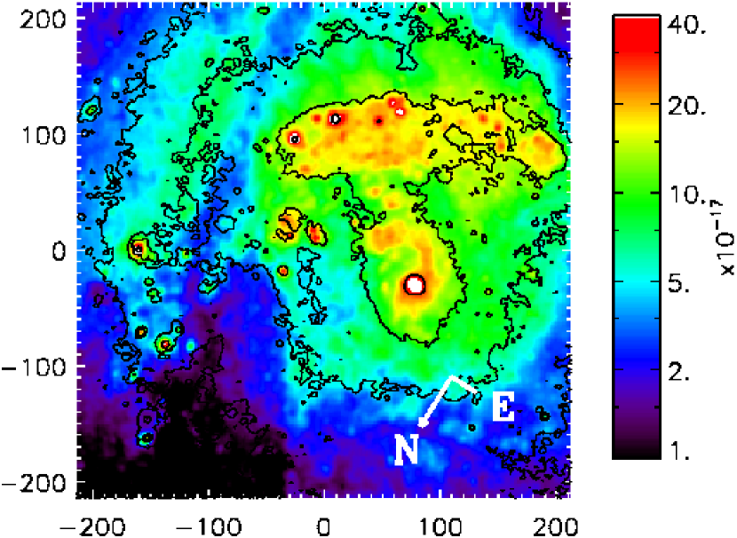
Figure 2: The homogenised WFPC2 F814W image, shown with logarithmic colour map scaling. Over-laid are contours of the homogenised NICMOS F222M image at levels $(1.3\times 10^{-15},1.8\times 10^{-15},2.5\times 10^{-15},7.4\times 10^{-15})$. The axes are scaled in pc and all fluxes are given in ergs s^-1 cm^-2. Note the accuracy of the spatial scaling and alignment between the WFPC2 and NICMOS data. The footprint of this image is shown in Fig. 1.

2.5 Synthetic Slits: merging space and ground based data

In order to merge the ISAAC data with the NICMOS and WFPC2 datasets, we extracted apertures from the HST data corresponding to the ISAAC slit positions. As the NICMOS and WFPC2 datasets were already homogeneous (§2.4), it remained to reproduce the seeing conditions and locate and extract synthetic slits.

To facilitate this procedure, a routine was written to minimise the $\chi^{2}$ difference between the ISAAC long-slit flux profile (short-ward of the CO bandhead at 2.3$\mu$m) and a flux profile produced by overlaying a 0$\aas@@fstack{\prime\prime}$6 slit aperture on the NICMOS F222M image, incorporating sub-pixel shifting, rotation and Gaussian convolution to emulate the seeing conditions. The problem was highly non-linear, with many local minima which could stall the process. Thus the optimisation required a good initial guess for the parameters (made by eye).

The principal result of this routine was the extraction of series of synthetic slits from the HST images, aligned to the ISAAC data and matched in spatial resolution. A by-product was an accurate estimate for the seeing of the ISAAC ground-based data (Table 1) which allows for greater accuracy and less contamination when extracting spectra of individual star clusters (§3.1). The reported seeing from the Differential Image Motion Monitor (DIMM) did not always represent the true seeing of our data, which is not surprising given that the DIMM looks in a roughly fixed direction (Sarazin & Roddier, 1990, less than $30\deg$ from the zenith) and at visible wavelengths; the ISAAC data was taken at a different position on the sky, with a different airmass and in the NIR (recall that seeing $\propto\lambda^{-0.2}$).

3 Data Analysis

We wish to build on the study of H01 and compare optical and NIR indices for clusters in the circumnuclear arc with stellar population models and also address the claims of T00 and D06 regarding the presence of a second obscured mass concentration. The first of these goals requires chemical and kinematic analysis of individual clusters. The latter requires kinematic analysis along Slit A (or B): Fig. 3 illustrates the positions of the putative hidden mass concentrations and our ISAAC long-slit data.

We discuss such analysis below, in two sections: one for ground based VLT ISAAC spectra and one for the space-based imaging.

3.1 VLT/ISAAC data

The ISAAC K-band long-slit spectra hold both kinematic and chemical abundance information. We discuss the extraction of this information from the ISAAC spectra after presenting details of our apertures.

3.1.1 Cluster Apertures

To study the properties of the individual star forming clusters at the centre of M83, individual spectra were extracted from the long-slit ISAAC spectra. To maximise the SNR and minimise contamination from background stars and nearby knots, apertures were centred on the peak flux with widths equal $2\sigma$ (§2.5). However, the poorer seeing-limited resolution of the ground-based ISAAC spectra sometimes resulted in the blending of clusters and the corresponding spectra. This is made clear in Table 4 for clusters that are resolved into multiple components at HST resolution. Most of the clusters seen in the K-band spectra are clearly coincident with those detected in H01. However, some are not; they were too heavily obscured by dust to be detected in the visible. Table 4 identifies clusters already identified in H01.

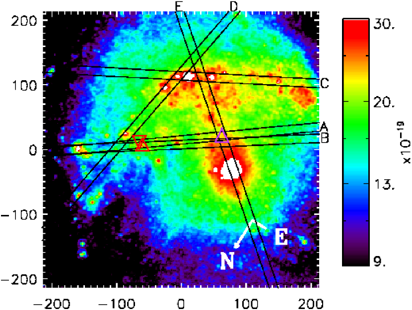
Figure 3: The 5 slit positions overlaid on the F222M NICMOS image. Positions of the putative hidden mass concentrations are also shown as purple (T00) and red (D06b) triangles. For the latter position, two triangles are plotted: the upright triangle gives the position determined from the astrometry while the inverted triangle gives the position estimated directly from the figures of D06b (see §4.6). Flux values are given in ergs s^-1 cm^-2. The position, scaling and orientation is the same as Fig. 2.

3.1.2 Stellar Kinematics

The stellar kinematics were extracted both for individual clusters and along the whole slit using a Direct Pixel Fitting technique (based on that of Rix & White 1992 and described in detail in Houghton et al. 2006).

The library of stellar templates used to extract the kinematics contained 20 stars: 6 giants (K1III to M6III) and 14 supergiants (K4I to M5I). To accurately extract kinematics of a young population (flux dominated by supergiants), it is essential to have a large number and range of supergiant templates to minimise template mismatch. This is particularly important for the CO ro-vibrational absorption after 2.3µm because the depth of the features is strongly dependent on the spectral type and there is more intrinsic scatter in the supergiant relation compared to that of giants (Kleinmann & Hall, 1986; Origlia et al., 1993). The stellar kinematics were extracted in the range 2.254µm- 2.355µm (a limit imposed by the stellar templates observed with the 0$\aas@@fstack{\prime\prime}$3 slit as described in §2.1 and by the need for good data away from the detector edge).

When extracting stellar kinematics along the entire slit, it was sometimes necessary to bin-up the data; we chose to bin the spectra to a minimum SNR of 20 (in the continuum, just before the CO bandhead at 2.295µm).

3.1.3 Gas Kinematics

The neutral gas kinematics of the H₂ 2-1 S(1) emission line ($\lambda_{\textrm{vac}}22477.17\textrm{\AA}$, Hinkle et al., 2000) were also extracted along the slits. This emission does not coincide with the wavelength range used to extract the stellar kinematics, preventing us from extracting them simultaneously (Sarzi et al., 2006). We instead fitted a Gaussian profile and linear continuum to the range 2.243µm - 2.258µm (-500km s^-1 to +1500km s^-1 in velocity; approximately $\pm$1000km s^-1 from the average gas velocity).

3.1.4 W[CO]

We measured the equivalent width of the first CO band ($\mu=2\to 0$), W[CO] (as defined by Origlia et al., 1993) from the ISAAC K-band spectra. W[CO] was calculated in the traditional sense,

$$\textrm{W}=\sum_{i}\Big{[}\frac{f_{i}}{c_{i}}-1\Big{]}\delta\lambda,$$ (1)

where $f_{i}$ is the observed (line and continuum) flux of each bin, $c_{i}$ is the (estimated) continuum flux of each bin, $\delta\lambda$ is the width of each bin (in Å) and $i$ indexes a suitable wavelength range.

However, Oliva et al. (1995) showed that the measured W[CO] of a galaxy is affected by the dispersion of the system. We corrected for this using the same technique as in Houghton et al. (2006): we artificially broadened the stellar kinematic templates, fitted a second order polynomial to the mean result and then applied a correction using the measured stellar velocity dispersion of the cluster. However, for the most part, this has negligible effect on W[CO] due to the very low dispersions of the star clusters.

3.2 HST/NICMOS and HST/WFPC2 data

3.2.1 Extinction map

Using the homogenised H$\alpha$ (WFPC2) and Pa$\alpha$ (NICMOS) images, we were able to calculate a deep extinction map for the centre of M83 as well as for individual clusters. We used a standard Milky Way extinction curve (Cardelli et al., 1989), recombination ratios of Osterbrock (1989) and a ratio of total to selective extinction, R${}_{\textrm{\scriptsize V}}$, of 3.1 to calculate the extinction $\textrm{A}_{\textrm{\scriptsize V}}$. Thus we find:

$$\textrm{A}^{gas}_{\textrm{\scriptsize V}}=3.1~{}\textrm{E}(B-V)^{gas}=-1.6\ln{\left[\frac{\textrm{F}_{\textrm{\scriptsize H}\alpha}/\textrm{F}_{\textrm{\scriptsize Pa}\alpha}}{8.13}\right]}$$ (2)

where $\textrm{F}_{\textrm{\scriptsize H}\alpha}$ and $\textrm{F}_{\textrm{\scriptsize Pa}\alpha}$ are the line fluxes of the H$\alpha$ and Pa$\alpha$ emission, respectively. The superscript ‘gas’ identifies that this term has been calculated from the ionised gas. Calzetti et al. (1994) found a substantial difference in optical depths between the H$\alpha$ and H$\beta$ Balmer emission lines and the stellar continuum underlying these two Balmer lines (in starburst galaxies). This was interpreted as a consequence of the hot ionising stars being associated with more dustier regions than the bulk stellar population. Our $A^{gas}_{V}$, determined from the H$\alpha$:Pa$\alpha$ decrement, will suffer a similar effect and we interpret it as the extinction suffered by the ionised gas, not the extinction of the (continuum producing) stellar population. For brevity, we now drop the superscript gas in $\textrm{A}_{\textrm{\scriptsize V}}$ and $\textrm{E}(B-V)$.

Figure 4 illustrates the extinction map. A substantial fraction of the pixels in the map have no secure upper limit; that is to say, within $2\sigma$ errors, they are unconstrained. A similar result evident in Fig. 8.

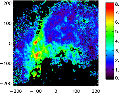
Figure 4: The extinction $\textrm{A}_{\textrm{\scriptsize V}}$ calculated from the H$\alpha$:Pa$\alpha$ ratio. The position, scaling and orientation is the same as Fig. 2. Only pixels with $2\sigma$ detections in either the H$\alpha$ or Pa$\alpha$ fluxes are shown (pixels not matching this criterion are coloured black). A substantial fraction of these pixels have no secure upper bound on the extinction value, within the $2\sigma$ errors; almost none have a secure upper limit within $3\sigma$. This is a result of the low SNR of the NICMOS Pa$\alpha$ data.

3.2.2 Cluster Apertures

Apertures with the exact same size and position as those for the ISAAC data (§3.1.1) were extracted from the synthetic HST slits (§2.5), to calculate the equivalent widths of the Pa$\alpha$ and H$\alpha$ emission for individual clusters.

As W[H$\alpha$] and W[Pa$\alpha$] were derived from homogenised narrow band images, we calculate an approximation to the true equivalent width, namely

$$\textrm{W}\simeq\Big{[}\frac{F_{\lambda}-C_{\lambda}}{C_{\lambda}}\Delta\lambda\Big{]},$$ (3)

where $F_{\lambda}$ is the observed flux density (line and continuum) of the narrow band image, $C_{\lambda}$ is the flux density of the continuum and $\Delta\lambda$ is the bandwidth of the narrow band filter.

These indices also require correction. As mentioned previously, when studying starburst galaxies, Calzetti et al. (1994) found different optical depths for the H$\alpha$ and H$\beta$ Balmer emission lines and the continuum underlying these two Balmer lines. Consequently, the observed equivalent widths of ionised gas emission are affected by this differential extinction between gas and stars and require correction before comparing to models.

Using the prescription described in Calzetti (1997) and Calzetti (2001), the extinction corrections for W[H$\alpha$] and W[Pa$\alpha$] were calculated to be

$$\log{\left[\frac{\textrm{W}(\textrm{H}{\alpha})_{o}}{\textrm{W}(\textrm{H}{\alpha})_{i}}\right]}=-0.4~{}\textrm{E}(B-V)$$ (4)

$$\log{\left[\frac{\textrm{W}(\textrm{Pa}{\alpha})_{o}}{\textrm{W}(\textrm{Pa}{\alpha})_{i}}\right]}=-0.04~{}\textrm{E}(B-V)$$ (5)

where $\textrm{W}_{o}$ is the observed equivalent width, $\textrm{W}_{i}$ is the intrinsic width and $\textrm{E}(B-V)$ is calculated from the H$\alpha$:Pa$\alpha$ decrement using a ‘standard’ extinction curve (§3.2.1). The errors in the corrected values were nearly always dominated by the error in $\textrm{E}(B-V)$.

3.3 Starburst99 Ages

SB99 models enable us to age-date individual knots seen in the star forming region of M83. We use three indices for this purpose: W[CO] direct from the stellar population and W[H$\alpha$] and W[Pa$\alpha$] from the gaseous nebula emission (which essentially measure the same quantity, but differ due to the effects of extinction). W[CO] is defined according to Origlia et al. (1993) in both SB99 and our measurements. Although W[CO] is affected by the spectral resolution of the observations, the low resolution of the SB99 model spectra in the NIR is not an issue because SB99 calculates W[CO] from expanded versions of the (higher resolution) Origlia et al. (1999) models, which in turn implement the theoretical equivalent widths from Origlia et al. (1993).

Although many nebula emission indices are calculated by default in the SB99 models, W[Pa$\alpha$] is not. Therefore, we follow the prescription of Leitherer & Heckman (1995, and references therein) and calculate it directly from the number of ionising photons (with wavelength $<912$Å) and the model Pa$\alpha$ continuum at 1.876$\mu$m as a function of time.

3.3.1 SSP models

Simple instantaneous single stellar population (SSP) burst models for W[Pa$\alpha$] and W[CO] (Fig. 5, dashed lines) were calculated with a Salpeter IMF ($\alpha=2.35$), a mass range of 1$\textrm{M}_{\odot}$$<M_{\star}<100$$\textrm{M}_{\odot}$ and for a metallicity $Z=2Z_{\odot}$ (Kobulnicky et al., 1999, appropriate for M83) using the Geneva tracks (Meynet et al., 1994). No W[CO] is expected before 6 Myrs, which is the point at which the massive stars of a SSP first evolve to the red super-giant (RSG) phase; this property is relatively insensitive to variations in $M_{\textrm{\scriptsize up}}$ between 30 and 100 $\textrm{M}_{\odot}$ because of the small number of RSGs evolving from progenitor masses above 30 $\textrm{M}_{\odot}$ (Origlia et al., 1999). These SSP models were found to be incompatible with our data for individual clusters: W[Pa$\alpha$] gave consistently younger ages compared to W[CO], by order of a few Myrs. If the RSG phase was occurring earlier than predicted by the models, one would expect all W[CO] measurements to be $>15$ as the time period for which young stars have $0<$ W[CO] $<15$ is very small. We therefore inferred that the variation in W[CO] comes from a mixed population, of stars that have evolved to the RSG and stars that have not, which in turn implies a mix of ages and a finite formation timescale for the clusters.

3.3.2 Mixed population models

SB99 models only provide two cases of the star formation law: an instantaneous burst or constant star formation. We therefore investigated the effect of different formation scenarios using the first of these limiting cases. In particular we investigated the evolution of a short, finite episode of star formation. Similar star formation laws (albeit for exponential bursts) were investigated in Förster Schreiber et al. (2003), but using different models and data.

All indices for the mixed population were calculated by convolving SSP model fluxes (or flux densities) over time with a suitable kernel. Convolution with a top hat kernel thus mimicked a finite episode of constant star formation. W[Pa$\alpha$] was calculated by convolving the number of ionising photons of a SSP and the related model continuum flux density at 1.876$\mu$m with the desired kernel. We then calculate W[Pa$\alpha$] as before using these new mixed population values. When calculating W[CO], we first converted it into a flux using the model continuum at 2.29$\mu$m. This wavelength-integrated flux and the same SSP continuum at 2.29$\mu$m were then convolved with the desired kernel and used to recalculate W[CO] for the mixed population.

Fig. 5 shows W[Pa$\alpha$] and W[CO] for an episode of continuous star formation lasting 6 Myrs (solid lines). The effect of a finite duration star formation on W[Pa$\alpha$] is clearly negligible, but the onset of the W[CO] index is brought forward in time by a few Myrs. As expected, after around 10 Myrs, the SSP and mixed population models are indistinguishable as changes in the indices become slower and less pronounced. The mixing timescale of 6 Myrs is somewhat arbitrary and was chosen by eye to to best fit the data. Formal errors are difficult to estimate, although the data appears to be inconsistent with timescales less than 5 Myrs and larger than 7 Myrs, giving a 1 Myr margin.

Strictly speaking, we cannot perfectly reproduce a finite duration of constant star formation from instantaneous burst models; rather, we are in fact producing a mixed population via many sequential instantaneous bursts over a finite duration and assuming that this closely approximates a short episode of constant star formation. The time resolution for the mixing (separation between the sequential SSP models) is 0.1 Myrs. We see no significant change with smaller time resolutions and so presume that we closely approximate the ideal case of continuous star formation over a finite time.

Using the same techniques, we investigated the effect of the functional form for the star formation during the finite episode and found reasonable fits for a finite burst of exponentially increasing star formation (e-folding time $\sim 3$Myrs) and a finite burst of exponentially decaying star formation (e-folding time $\sim 2$Myrs). Although the finite episode of constant star formation always provided an overall better fit, our data was not able to reliably distinguish between such alternatives, so we chose to adopt the simplest scenario (i.e. a short burst of constant star formation). We also tested the effect of contaminating an SSP model with an old (Gyr) population and such a scenario could not reproduce the observed data trends: the W[CO] estimates were too high for the younger clusters (i.e. those with high W[Pa$\alpha$]). Finally, we tested multiple SSP bursts separated by the dynamical timescale and half the dynamical timescale, motivated by the work of Allard et al. (2006); Sarzi et al. (2007) and Falcón-Barroso et al. (2007) and our attempts mostly suffered the previous problem: too much W[CO] at younger ages. However, although many episodic bursts (i.e. more than 2) were unsuccessful at reproducing the observed data trends, models with only two burst were more successful: fine tuning the mass fraction of the latter burst to be 3 – 4 times the initial burst mass, setting the delay between the bursts to 5 Myrs and diluting the W[CO] with a fraction of the total luminosity to mimic hot dust emission (somewhat simplistic compared to the models of Förster Schreiber et al. 2003) and replacing the SSP bursts with finite (Myr) bursts went some way to reproducing the data but did not completely resolve the discrepancy. Thus, despite considerable fine tuning of various parameters, multiple bursts did not match the data as well as a constant burst lasting 6 Myrs.

SB99 was recently updated to offer models based on either the Geneva (Meynet et al., 1994) or the Padova tracks (Fagotto et al., 1994). Although we illustrate models using both the Geneva and Padova tracks in Fig. 5, we use Geneva tracks to estimate the ages of the clusters in the final analysis (the same as H01); the Padova tracks with a similar metallicity (2.5Z_⊙) still match the data and provide a similar age gradient, but with a tendency for younger ages. This is explained by the slightly earlier onset of W[CO] in Fig. 5 when using the Padova tracks.

It is not trivial to read the cluster ages from an age-metallicity grid such as Fig. 6: if one allows variation in the metallicity, there is a larger range of acceptable ages given the age-metallicity degeneracy. As the random errors in W[Pa$\alpha$] are usually much larger than those of W[CO], one could use a fixed metallicity ($2Z\mbox{${}_{\odot}$}$) and take the nearest age along the horizontal but such an approach is unfeasible when the error for W[Pa$\alpha$] is small compared to the horizontal distance to the nearest model track (as is the case for cluster 8). We derived ages from models of a fixed metallicity ($2Z\mbox{${}_{\odot}$}$) using the shortest line from the observation to the $2Z\mbox{${}_{\odot}$}$ model tracks along W[Pa$\alpha$] and W[CO], effectively ignoring the larger uncertainty in W[Pa$\alpha$] and any variation in metallicity. We show the $Z\mbox{${}_{\odot}$}$ models (and how they link with the $2Z\mbox{${}_{\odot}$}$ models) in Fig. 6 to justify our metallicity assumption: most of the clusters scatter around the $2Z\mbox{${}_{\odot}$}$ tracks.

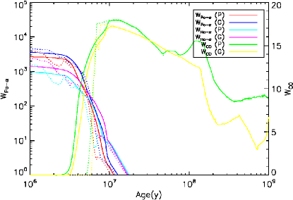
Figure 5: W[Pa$\alpha$] and W[CO] predictions from SB99 with $\alpha=2.35$ and M${}_{up}=100$$\textrm{M}_{\odot}$. Dotted lines represent the instantaneous burst models. Solid lines represent mixed models for a finite burst of constant star formation over 6 Myrs. The time scale on the plot is relative to the mid-point (mass weighted mean) of the burst. Models for both Geneva (G Meynet et al., 1994) and Padova (P Fagotto et al., 1994) tracks are shown, thanks to the recent update to SB99 (Vázquez & Leitherer, 2005).

4 Errors

The estimation of errors in our datasets deserves special mention as they sometimes required care and are not always calculated using the standard first-order approach, for good reason.

4.1 Homogenised HST data

By homogenising the HST datasets, we introduced correlations between the pixels and between the errors. Whenever we added pixels, we added the variances. This would usually cause our errors to be severely underestimated given that the variances become correlated and would not add in such a manner. However, careful scrutiny of our method using Monte-Carlo simulations of noise frames actually indicates that our final random errors are over-estimated by a minimum factor of $\sim 1.7$. The cause is the seeing convolution stage: we simply convolve our variance arrays in the same manner as the data, but this only results in obtaining a seeing weighted average variance for each input pixel; in reality, the true error is reduced much more than this. Thus, the greater the seeing, the larger our over-estimation of the errors. We estimate factors of (1.7, 1.9, 1.9, 2.9) for slits (A, B, C, D), respectively but we do not apply these corrections.

One could question why we degraded the H$\alpha$ and Pa$\alpha$ data to match the spatial resolution of the ground-based data: we could obtain better spatially resolved data for these indices. However, then one is faced with the dilemma of combining non-homogeneous data and which to trust. The final spatial resolution of our data is thus limited by the seeing, but it is worth recalling the resolution of the study by H01, which is only a factor of two better. Although the diffraction limited FWHM of HST at 656nm is 0$\aas@@fstack{\prime\prime}$056, the pixel sampling of WFPC2 is 0$\aas@@fstack{\prime\prime}$04554. However, H01 further convolved the data with a Gaussian of $\sigma=2$ pixels (FWHM = 0$\aas@@fstack{\prime\prime}$21) to create sufficiently uniform cluster profiles that could be well fitted by a single PSF model. This brought the final spatial resolution of the HST data to 0$\aas@@fstack{\prime\prime}$22. The resolution of our best data is 0$\aas@@fstack{\prime\prime}$4 — only a factor of two larger. Furthermore, H01 calculated W[H$\alpha$] within 0$\aas@@fstack{\prime\prime}$56 and 1$\aas@@fstack{\prime\prime}$34 diameter apertures (12pc and 29pc at 4.5Mpc) and found little difference between them for most clusters. Our apertures are generally within this range: they are rectangular with heights equal to the slit width (0$\aas@@fstack{\prime\prime}$6) and widths equal to (0$\aas@@fstack{\prime\prime}$3, 0$\aas@@fstack{\prime\prime}$4, 0$\aas@@fstack{\prime\prime}$4, 1$\aas@@fstack{\prime\prime}$1) for slits (A, B, C, D), as determined by the seeing. We choose to use the higher resolution of the space-based data only to flag potentially contaminated (unresolved) data in Table 4. Thus we measure luminosity weighted ages for any contaminated clusters which may be particularly true for clusters 5, 8 and 12 in Table 4.

4.2 W[CO]

If we calculate the random error in W[CO] from error in the flux values alone, we find that it is negligible compared to the error introduced by uncertainly in the velocity and dispersion. Therefore, we use $\pm 1\sigma$ random errors in the velocity and velocity dispersion measurements of each cluster to calculate the systematic error in W[CO]. We then use whichever is the larger. As a result, the error in W[CO] is often asymmetric.

4.3 H$\alpha$

As discussed in §2.3, the H$\alpha$ flux is subject to an uncertainty in the gas velocity due to the systematic velocity of M83 placing the emission on the edge of the F656N bandpass. We therefore appoint minimum errors of 10% to all H$\alpha$ fluxes (often dominating the error in W[H$\alpha$] for the clusters) and in calculating the extinction estimate of Fig. 8. This 10% systematic error corrects for velocity range of 430km s^-1 to 560km s^-1. Because this error is systematic, it does not change with binning or aperture size and is applied as a last step before analysis.

4.4 $\textrm{A}_{\textrm{\scriptsize V}}$, $\textrm{E}(B-V)$

Extinction estimates using a HII decrement are often tricky due to the uncertain penetration depth of the emission lines in question: estimating the extinction in dusty regions using the H$\beta$:H$\alpha$ decrement invariably leads to a lower estimate than comparing the H$\alpha$:Pa$\alpha$ decrement as the effective penetration is much greater with the Pa$\alpha$ line. We assume that our H$\alpha$:Pa$\alpha$ decrement is not limited in this way for the range considered here $(0<$$\textrm{A}_{\textrm{\scriptsize V}}$$<8)$. However, estimating the random error is still non-trivial.

A standard first-order approach gives that the error in Eq. 2 is $\sigma_{A_{v}}=-1.6({\textrm{F}_{\textrm{\scriptsize Pa}\alpha}}/{\textrm{F}_{\textrm{\scriptsize H}\alpha}})$. However, this is only valid for small errors in ${\textrm{F}_{\textrm{\scriptsize Pa}\alpha}}$ and ${\textrm{F}_{\textrm{\scriptsize H}\alpha}}$: the errors in Pa$\alpha$ data are large (sometimes $\gg 10$%) and the approximation breaks down. We therefore calculate the error explicitly by substitution. Due to the non-linear nature of Eq. 2, there is considerable difference between the $1\sigma$ and $2\sigma$ confidence limits. We therefore opt to quote $2\sigma$ values because $1\sigma$ values are significantly smaller and lead to a false impression of accuracy. The errors in the corrected W[H$\alpha$] and W[Pa$\alpha$] of Fig. 6(c) and (d), dominated by the error in $\textrm{A}_{\textrm{\scriptsize V}}$ were calculated using this $2\sigma$ error.

4.5 Cluster Ages

We wish to quote an error for the ages of the clusters, but this is not trivial. Here, we list the reasons for the difficulty and explain how the age errors in Table 4 are determined.

The cluster ages are calculated from the NIR indices W[Pa$\alpha$] and W[CO]. The NIR indices (particularly W[Pa$\alpha$]) suffer less from extinction and are therefore more accurate in terms of random error and also any systematic error associated with the extinction correction (e.g. the extinction law, the unknown penetration depth of our H$\alpha$ and Pa$\alpha$ data) because the correction is smaller. W[CO] is corrected for velocity dispersion effects but this correction is very small and does not affect the derived ages. However, young clusters are expected to be dusty and if heated by UV radiation, this dust re-emits, mainly in the mid-IR but also in the NIR which could diminish the W[CO] index by artificially increasing the continuum level and thus affect our derived ages and the mixing timescale of §3.3.2; however, this effect is usually very weak and we do not attempt to correct our data for this effect, unlike the study by Förster Schreiber et al. (2003).

The choice of evolutionary tracks also plays a role: we quote ages using the Geneva tracks, but the Padova tracks also fit the data albeit with systematically lower ages of around 0.5 Myrs for the youngest clusters (4.5 Myrs old) and 1.5 Myrs for the oldest clusters in the arc (8 Myrs old). This difference leads us to quote a systematic uncertainty in our age estimates of order $\pm 1$Myr.

We also vary the mixing timescale of the models to match the cluster data (§3.3.2). The mixing timescale was chosen by eye to fit the observations, which were inconsistent with mixing timescales less than 5 Myrs or larger than 7 Myrs. Error in this parameter will manifest itself as a systematic error in the ages, particularly for the youngest clusters as this is where the change is greatest. We also note that without applying the Calzetti et al. extinction law, the data of Fig. 6(a) is best fit by a burst duration of 5.5 Myrs. Thus, given that the mixing timescale is estimated to be accurate to a Myr, we estimate the youngest clusters could also suffer another systematic error of order $\pm 1$Myrs.

We are also somewhat limited by our ground-based spatial resolution. Because we homogenise all our data, this affects W[H$\alpha$], W[Pa$\alpha$] and W[CO] and the derived ages. If two clusters are unresolved, we expect to measure a luminosity weighted W[H$\alpha$], W[Pa$\alpha$] and W[CO]. But whereas younger clusters ($<5$ Myrs) will have higher H$\alpha$ and Pa$\alpha$ emission (after correcting for extinction), the K-band luminosity and the W[CO] is dominated by older (10 Myr) clusters. Hence if the two unresolved clusters are different in age, we obtain conflicting ages from the different indices. However, one expects neighbouring clusters to have similar ages (given the results of H01), so this effect is probably small. Nevertheless, it is possible to identify contamination from another cluster or from the bulge stars (for highly extinct, dim clusters). The luminosity weighted stellar velocity dispersion of low mass star clusters is very low ($<20$km s^-1), so if we measure them to be high ($>30$km s^-1), the K-band light is likely not dominated by a single cluster. Consequently, when a cluster has a large velocity dispersion ($>30$km s^-1), it is noted in Table 4. Furthermore, when extracting the kinematics of each cluster, we fit a linear combination of stellar templates. As discussed in §2.1, we have a large number of giant and supergiant templates to fit the spectra and the best-fit template can be used to indicate the different stellar populations in the spectrum, and the relative fractions. Therefore, in Table 4 we give the fraction of giant and supergiant stars used to create the best-fit kinematic template for each cluster. The giant/supergiant fraction clearly correlates with the velocity dispersions and we can identify which cluster measurements are contaminated, and to what degree. What effect the fraction of contamination has on the derived ages is not always obvious, but is likely to lead to bias towards the age of the contaminant; thus we quote the ages (from H01) of any contaminating clusters resolved in HST images in Table 4 so that the reader can compare the measured age of the cluster with the measured age of the contaminant(s).

Finally, we have to match the observed cluster data with the models. Given the age-metallicity degeneracy, this is not trivial and we discuss our method in §3.3.2. The proximity of our observations to the nearest point on the $2Z\mbox{${}_{\odot}$}$ model track is an indication of how well the model fits the data, but it is also an indication of the stochastic nature of star formation: given a continuous IMF and only a relatively small quantity of gas, the stars formed will not be uniformly distributed over the entire mass range but will be scattered at random positions weighted by the IMF (especially true for the red supergiants). Thus we expect an intrinsic scatter in the number of red supergiants per cluster given a known mass and age, which leads to an intrinsic scatter in the observable quantities W[Pa$\alpha$] and W[CO] — they will never agree perfectly with the models. Given that H01 estimate most of the clusters to have masses around $10^{4}$–$10^{5}$M_⊙, we must consider these stochastic processes. For the majority of cases, the agreement between data and models is very good which leads us to estimate a random error of 0.5 Myrs for most of the clusters. However, there are some clusters which are more difficult, such as 8 and 10; for these clusters we do not know if error (systematic or random) or nature has resulted in the data falling far from the models. Somewhat arbitrarily, we assign random errors of $\pm 1$Myr to these clusters. For clusters that do not match the model predictions for both W[Pa$\alpha$] and W[CO] (clusters 14 and 15) we choose to trust the W[CO] index (see §5.1) but assign asymmetric errors to cover the range of all possibilities. For clusters that are do not match the models and are assumed to be very old ($>10$Myrs) we do not quote an error, only a lower limit.

4.6 Astrometry

Fig. 3 shows the positions of the putative hidden mass concentrations relative to the NICMOS data and the ISAAC slits.

The slits were located on the NICMOS image as described in §2.5 and were not positioned using the astrometry provided with the ISAAC and NICMOS data. Formal uncertainties are difficult to calculate although by trial and error, we estimate the error in $x$ and $y$ for Slit A to be at around 0$\aas@@fstack{\prime\prime}$1 (comparable to a NICMOS pixel) and the error in the position angle to be at most $1\deg$. However, these values vary for each slit: with poorer seeing, the ISAAC data is smoother and the errors in the slit positions increase slightly.

The pipeline reduced WFPC2 and NICMOS images come with world coordinate systems. However, the two systems were not comparable: the cluster positions of H01 were correctly centred on the WFPC2 images (as to be expected, for they were derived from the same data) but they were offset when overlaid on the raw NICMOS images (0$\aas@@fstack{\prime\prime}$54 to the SE as determined from the position of the nucleus in the raw F814W image and the raw F222M image). We chose the path of least resistance and adopted the WFPC2 astrometry. To calculate a world coordinate system for our homogenised data, we used our precise knowledge of the pixel size of the homogenised HST data (square pixels with sides 0$\aas@@fstack{\prime\prime}$0752963 in length) and varied the absolute reference to best align the positions of the clusters from H01 on the data. We assumed no error in the position angle of the WFPC2 and NICMOS data as defined by the ORIENTAT header keyword. Comparing our astrometry, we find the nucleus at (13h37m00.91s, -29d51m55.7s) whereas D06b find it at (13h37m00.95s, -29d51m55.5s): an offset of 0$\aas@@fstack{\prime\prime}$49 to the NE.

With no agreement between the WFPC2, NICMOS or D06b astrometry, we retain that of the WFPC2 images. However, when plotting the position of the hidden mass concentration given in D06b we apply a shift of 0$\aas@@fstack{\prime\prime}$49 to the SW - the same shift which would align the position of the nucleus given by D06b to the position of the nucleus in our world coordinate system (WCS). Quite by chance, more than by design, this places the position of the putative mass concentration securely in the middle of Slit A. However, D06b state a $2\sigma$ error of 0$\aas@@fstack{\prime\prime}$7 in their coordinates for this position; our slit width is 0$\aas@@fstack{\prime\prime}$6. Thus, it is reasonable to argue that the absolute centre of the proposed mass concentration could still lie outside our slit position; however it is unreasonable to argue that we wouldn’t detect its gravitational influence in the stellar kinematics given that the gas kinematics appear kinematically disturbed over many arcseconds in data of D06. For completeness, in Fig. 3 we also plot the position of the D06 interloper using their images as a reference, rather than their coordinates; this second location still overlaps that of Slit A but is approximately 0$\aas@@fstack{\prime\prime}$38 (8pc) west of the formal position in our WCS.

The position of the mass concentration proposed by T00 was considerably easier to locate: by using the position of the second dispersion peak in the original data and then locating the position of this slit on the homogenised HST data using the same techniques as for the other slits (§2.5), we were able to locate the second dispersion peak on the homogenised HST data without resorting to any WCS. By design, Slit A overlays this same position. We assumed that the second dispersion peak was centred along the slit width, which could be open to speculation. However, as Slit A is roughly perpendicular to the original slit of T00 (Slit E in Fig. 3), we would adequately cover any positional error perpendicular to the original slit.

5 Results

We present our findings with regard to the cluster ages and the putative hidden mass concentrations, in two appropriate sections.

5.1 Cluster Ages

Fig. 6(a) shows the mixed model predictions for the evolution of W[CO] and W[Pa$\alpha$] for solar (Z_⊙) and twice-solar (2Z_⊙) metallicity with data points for individual clusters over plotted. The same models and clusters are plotted in Fig. 6(b) for W[CO] and W[H$\alpha$]. As W[H$\alpha$] and W[Pa$\alpha$] are essentially measuring the same quantity (the number of ionising photons), the main difference between the two figures is the effect of extinction.

Green points indicate less extinct clusters ($\textrm{A}_{\textrm{\scriptsize V}}$$<2$), that roughly match the 2Z_⊙ mixed population models for W[Pa$\alpha$]  W[H$\alpha$] and W[CO], whereas the orange points indicate more extinct clusters ($\textrm{A}_{\textrm{\scriptsize V}}$$>2$), that tend only to match the model predictions for W[Pa$\alpha$] and W[CO] and lie below the predictions for W[H$\alpha$]. At first, W[H$\alpha$] and W[Pa$\alpha$] therefore appear to be uncorrelated in Fig. 6(a,b) but after applying Calzetti’s differential extinction, the correlation is obvious in Fig. 6(c,d). The duration of the star formation episode (6 Myrs) was therefore chosen to fit both the (corrected) W[H$\alpha$]-W[CO] and W[Pa$\alpha$]-W[CO] data in Figs. 6(c,d).

Red points indicate clusters that do not match model predictions in the (corrected) W[H$\alpha$]-W[CO] and the W[Pa$\alpha$]-W[CO] plots. Although only models with ages $<10$ Myrs are given in Fig. 6, these points are not consistent with older populations either, due to the larger values of W[H$\alpha$] and W[Pa$\alpha$]. However, two of these clusters (16 and 17 in Table 4) have very low W[H$\alpha$] and W[Pa$\alpha$] and it is therefore important to consider non-photoionised gas emission (caused primarily by shocks and their precursors, from supernovae and massive stellar winds but also turbulent mixing layers and changes in gas temperature as explained by Calzetti et al. 2004). Although these two clusters are not in the non-photoionised regions of M83 highlighted by Calzetti et al. (2004), one cannot discount the possibility of non-photoionised emission. As they are both quite distinct from the main star forming arc, we conclude that the H$\alpha$ and Pa$\alpha$ emission is non-photoionised and thus W[CO] reflects a much older population, greater than 10 Myrs. The other two red points (14, and 15 in Table 4) are somewhat puzzling (H01 also found the photometry of these clusters to be anomalous): either the nebula emission equivalent widths or the W[CO], or both, are low compared to the models. Comparing the ages predicted by each index, we noticed that the ages predicted by W[CO] were in good agreement with the ages of nearby clusters, but the ages predicted by W[H$\alpha$] and W[Pa$\alpha$] were not. Therefore we tentatively assign them ages based on W[CO] measurements alone (although cluster 15 is the only cluster entirely consistent with the instantaneous SSP models, it makes little difference to the derived age).

It should also be noted that clusters 5 and 12 are in a particularly densely populated region and their ages are likely more representative of the local average (of those clusters listed as contaminants in Table 4) because of significant contamination. Similarly, cluster 9 is probably heavily contaminated by cluster 13, although we do register significant differences in W[CO] for the two.

Fig. 7 illustrates the positions of the clusters with their ages (rounded to the nearest Myr) from Fig. 6(c), while Table 4 quotes them to the nearest 0.5 Myrs. Although the ages from Fig. 6(c) and Fig. 6(d) agree remarkably well for each cluster, we use the age derived from the NIR data (W[Pa$\alpha$]) because it is less effected by extinction and is therefore more accurate (as discussed in §4.5).

(a)

(b)

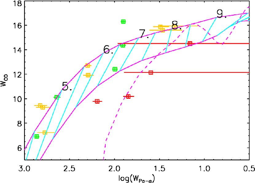
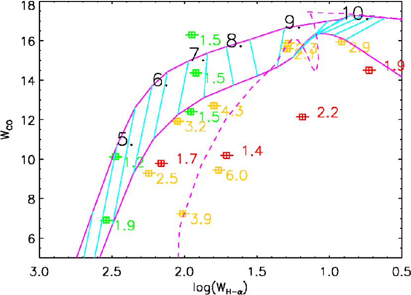
0

(c)

0

(d)

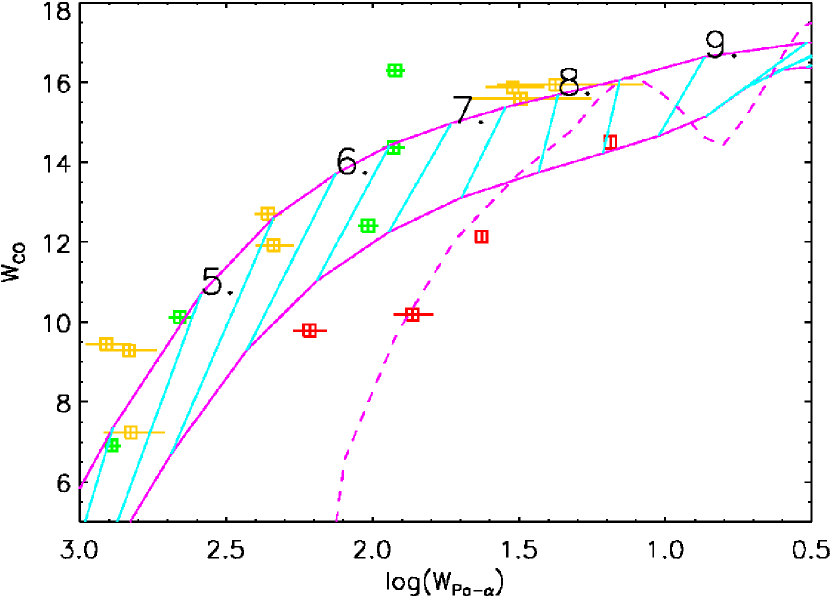
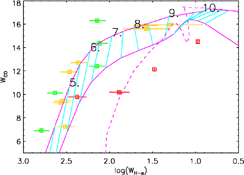
Figure 6: The SB99 models for the mixed population of Fig 5 with data points for individual star clusters. Unlike Fig. 5, two metallicities are shown: the top (magenta) curve shows models for Z=2Z_⊙ while the lower (magenta) curve shows models for Z=Z_⊙; the vertical blue lines link points of constant age and are spaced in 0.5 Myr intervals. Absolute ages are shown in Myrs on the upper (2Z_⊙) curve. The dashed (magenta) line gives the model predictions of the unmixed SSP (2Z_⊙). The data points represent measurements for individual clusters: green points indicate low extinction clusters consistent with ages $<10$ Myrs; yellow points indicate high extinction clusters consistent with ages $<10$ Myrs; red points indicate clusters that are inconsistent with ages $<10$ Myrs. The upper two panels, (a) and (b), show the extincted data; the lower two panels show the same plots with W[H$\alpha$] and W[Pa$\alpha$] corrected for differential reddening using the Calzetti prescription (§3.2.2). Panel (b) also quotes $\textrm{A}_{\textrm{\scriptsize V}}$for individual clusters. Horizontal error bars in the lower (extinction corrected) panels, (c) and (d), are often dominated by the uncertainty in the extinction: $2\sigma$ errors are shown for all clusters except for two red data points: the extinction, and therefore the corrected W[Pa$\alpha$] and W[H$\alpha$], are unconstrained within the $2\sigma$ errors, due to low H$\alpha$ and Pa$\alpha$ flux.

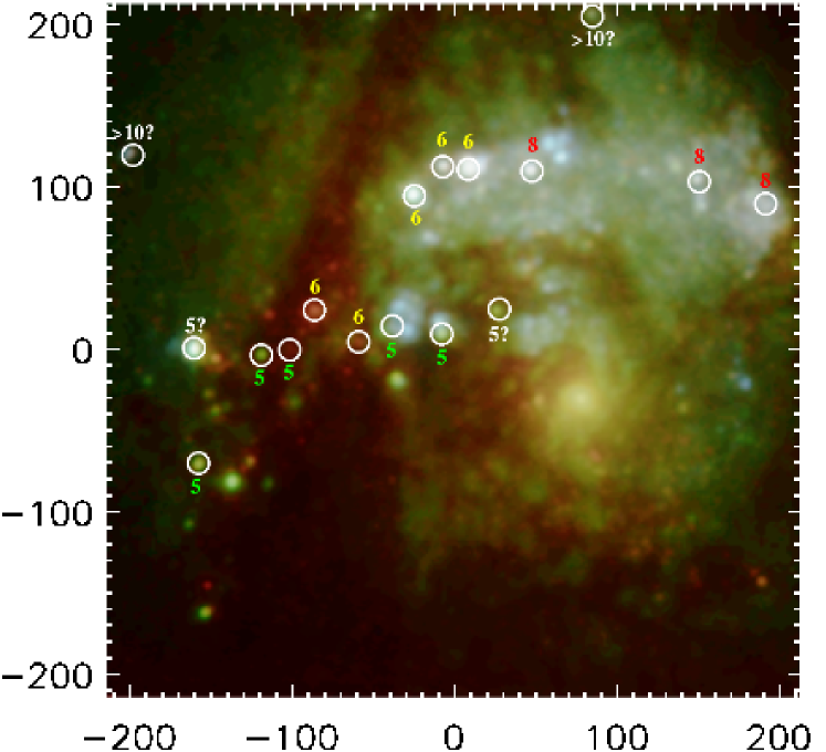
Figure 7: A false-colour image of the centre of M83 made with homogenised NICMOS and WFPC2 data. The position, scaling and orientation is the same as Fig. 2. NICMOS F222M is red, WFPC2 F814W is green and WFPC2 F300W is blue. A non-linear grey-scale has been employed to enhance low luminosity (heavily extinct) clusters. Note that the circumnuclear arc can be seen to extend into and along the dust lane. Cluster ages (derived from Fig. 6 and rounded to the nearest Myr) are over plotted: colours of the ages aid the eye in distinguishing the age gradient along the arc; green represents 5 Myrs, yellow represents 6 Myrs, red represents 8 Myrs while white represent uncertain ages. The resolution of this image is set by the NICMOS instrument and we estimate a FWHM of 0$\aas@@fstack{\prime\prime}$15.

5.2 Hidden Mass concentrations

Fig. 3 illustrates the positions of the putative hidden mass concentrations of D06 and T00 and our long-slit data. Both slits A and B show identical kinematic features at the location of D06b, therefore for brevity we show only the the kinematics along Slit A in Fig. 8.

A sharp gradient in the H₂ gas velocity $\textrm{V}_{\textrm{\scriptsize gas}}$ is found in the same vicinity that D06 report a gradient in the $\textrm{Pa}\beta$ gas velocity (140pc along slit A) and both gradients are in the same direction. The gradient in H₂ is sustained (i.e. $\textrm{V}_{\textrm{\scriptsize gas}}$ is roughly constant for 80pc to the north). There appears to be a gradient in the opposite direction at 60pc along the slit, although the line flux is low, the kinematics of Slit B disagree and there are luminous star clusters at this location which might bias the observations.

The stellar velocity $\textrm{V}_{\star}$ and stellar dispersion $\sigma_{\star}$ profiles both show synchronous drops in the vicinity of the D06 mass concentration (160pc along slit A), but these changes are not sustained and $\textrm{V}_{\star}$ and $\sigma_{\star}$ both recover, although the recovery is significantly more gradual on the north side.

All these features occur approximately at the edge of the north-east dust lane, clearly seen by plotting the extinction ($\textrm{A}_{\textrm{\scriptsize V}}$) along the slit in Fig. 8.

In Fig. 9, we show a position–velocity diagram for the stellar kinematics. The best-fit Gaussian line-of-sight velocity profiles (VPs) are shown at each position along the slit and each is scaled to the same maximum intensity for illustration purposes (i.e. the VPs are not normalised). Where it was necessary to bin the spectra to extract kinematics, the VPs in Fig. 9 are stretched accordingly. It appears from this figure that the changes in the stellar velocity and dispersion are synchronised with the sudden increase in the extinction via the dust lane. However, Fig. 9 suggests that the VPs extracted at the edge of the dust lane are principally affected at the high-velocity wing; the low-velocity side of the VP appears unaffected by the presence of the dust. In fact, if the kinematic fits are extended to include $h_{3}$ and $h_{4}$, we find very asymmetric VPs at the location of the dispersion drop with $h_{3}\sim 0.25$.

Further along the slit, we see a very small rise in the dispersion at the T00 location and the dispersion here is in agreement with that of the second dispersion peak in T00 of $\sim 70$km s^-1: there is no clear dispersion peak along this slit position.

Towards the south end of slit A (at around 340pc on Fig. 8) we see a further rise in $\textrm{V}_{\star}$ and $\sigma_{\star}$ accompanied by another strong gradient in $\textrm{V}_{\textrm{\scriptsize gas}}$. The extinction shows a marginal increase in roughly the same vicinity (320pc along the slit) but thereafter shows no obvious increase, although our errors for the extinction are unbound because of the very small H$\alpha$ and Pa$\alpha$ fluxes received here.

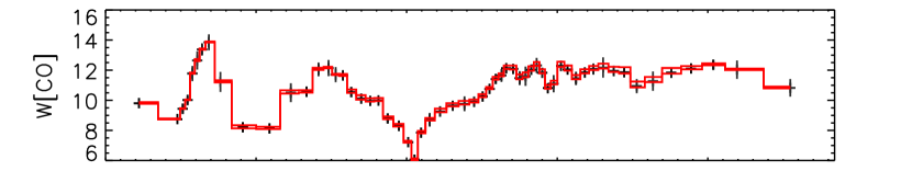
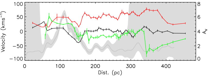
Figure 8: Upper panel: the flux profile of slit A. Positions of the putative hidden mass concentrations are also shown as purple (T00) and red (D06b) triangles. Middle panel: The W[CO] measured in each bin along slit A: red lines indicate maximum systematic errors from velocity and dispersion uncertainty; the error bars on the points correspond to random error. Lower panel: The Kinematics along slit A: the black, red and green lines illustrate the stellar velocity (relative to galaxy’s mean stellar velocity), stellar velocity dispersion and the H₂ gas velocity (also relative to galaxy’s mean stellar velocity), respectively; the grey line shows the extinction, $\textrm{A}_{\textrm{\scriptsize V}}$ calculated from the H$\alpha$ and Pa$\alpha$ emission and the lighter grey shading illustrates the $2\sigma$ error. Both panels: The PA of the slit is 126.95^∘, with the northern side on the left.

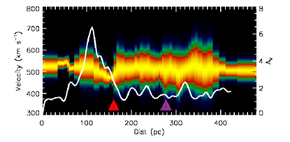
Figure 9: A position velocity diagram of the stellar kinematics from Fig. 8. Where it was necessary to bin the data to extract a VP, they have been stretched to represent the space over which the data was binned. The extinction profile $\textrm{A}_{\textrm{\scriptsize V}}$ of Fig. 8 is over plotted in white. Positions of the putative hidden mass concentrations are also shown as purple (T00) and red (D06b) triangles.

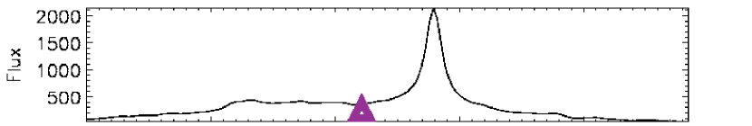
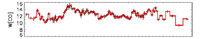
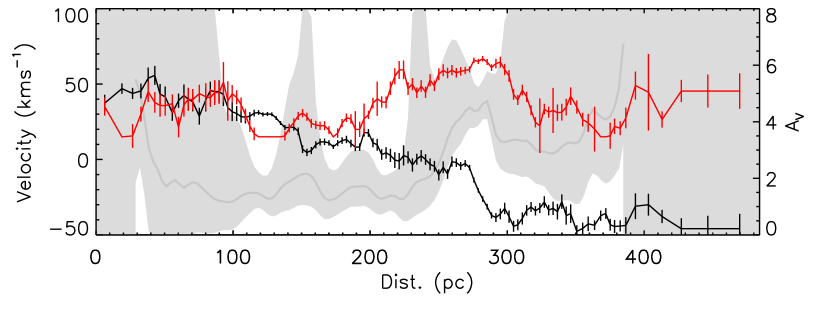
Figure 10: As for Fig. 8 but for slit E - the original data of T00. The position of the putative hidden mass concentration from T00 is shown as a purple triangle. Note that no H₂ gas velocity is shown in the lower panel due to its sparse detection along this slit.

Landscape table to go here - table4.ps

Table 4: BLANK

6 Discussion

Fig. 7 gives the clearest evidence yet of an age gradient along the circumnuclear arc, with the youngest clusters nearest (and coincident with) the north-east dust lane. The ages are generally in agreement with those found by H01, but with considerably less scatter. As done in D06b, if the H01 data is averaged over angular sections, then the age gradient is very similar to the one found here, although this work extends to the highly extincted clusters in the dust lane and the absolute ages are around a Myr older here.

We also see from the false-colour image of Fig. 7 that the star formation does not stop where the north-east dust lane intersects the arc, but continues through it and along the northern edge: there appear to be many star clusters at the young end of the arc, embedded in the dust lane. H01 considered the age gradient along the arc to be an indication of star formation propagating from the south-east end of the arc to the north-west, terminating roughly at the dust lane. D06 alternatively proposed that this propagation of star formation was a consequence of the dynamical friction trailing an interloping hidden mass concentration, such as a satellite galaxy (although see §6.1). However, we propose that the arc of young star clusters is a result of gas inflow along the north-east dust lane creating a nuclear spiral of gas and an associated ring of star formation, because we find no evidence to support the presence of an interloper at the position of D06(a,b) or the position of T00.

6.1 No hidden mass

Previous claims of hidden mass concentrations are inconsistent with our observations for many reasons which we outline below, in addition to the concerns raised in §1.5. We note that the strong gradient in the molecular gas velocity is 20pc north-west (left along slit A) of the formal position quoted in D06b for the hidden mass concentration. Whether this is a systematic error between coordinate systems or a genuine offset is unclear, although, as discussed in §4.6, close inspection of the figures in D06b provides a slightly different location, 0$\aas@@fstack{\prime\prime}$4 (8pc) west of the formal position, going some way to rectifying the difference.

A large mass concentration of the magnitude discussed in D06(a,b) would produce an observable rise in the velocity dispersion — as seen for the nucleus of similar mass (peak value $\sigma\sim$75km s^-1). We see no rise in the velocity dispersion at the location of D06 or at the location of the gradient in the molecular gas velocity. The highest stellar velocity dispersion seen at the position of the gradient in molecular gas velocity is $33\pm 2$km s^-1and just 15pc right along slit A is a minimum in the stellar velocity dispersion, measured to be $15\pm 3$km s^-1. This minimum in stellar velocity dispersion is probably caused by the young (6 Myrs) star cluster 5 in Table 4 but as we shall see, it is highly unlikely that this cluster is dominating the light from an extincted mass concentration. The minimum in stellar velocity dispersion may also be an effect of dust extinction: Baes et al. (2003) have shown that dust obscuration can lead to asymmetric velocity profiles and apparent drops in stellar velocity dispersion, although why we see the drop at the location of the shock and not at the peak of the extinction (some 50pc apart) is far from clear in this scenario.

At the location of the putative hidden mass concentration, the extinction ($\textrm{A}_{\textrm{\scriptsize V}}$) is 4$\pm$1 (2 sigma errors). This estimate is derived from the HII emission — the same tracer used to obtain the rotation gradient in D06(a,b). In the K-band, we therefore expect the extinction $\textrm{A}_{\textrm{\scriptsize K}}$ to be 0.4 magnitudes, so we will receive around two thirds of the total flux emitted from any stars co-spatial with the ionised emission (assuming foreground extinction). Yet we do not see any increase in surface brightness to indicate an increase in stellar density, other than cluster 5, which we measure to have a low stellar velocity dispersion of $\sim 15$km s^-1 and an age of 6 Myrs. Thus we conclude that there is no large ($\mbox{{\raisebox{-1.72218pt}{~{}$\stackrel{{\scriptstyle>}}{{{\scriptstyle\sim}}}$~{}}}}10^{7}$$\textrm{M}_{\odot}$) hidden mass there.

We, like H01, observe the youngest star clusters to preceded the trajectory of the putative mass concentration. This is contrary to Ostriker’s theory of dynamical friction in a gaseous medium and the subsequent hydrodynamical simulations as discussed in §1.5. These young clusters, as an extension of the arc, cannot be explained by invoking an interloping mass.

Shocks are well known to give rise to radio emission, as discussed in §1.2 and the MIR is well known to be correlated with the radio; thus the peaks observed in both wavebands near the position of the putative interloper are easily explained by a shock.

As for the other proposed hidden mass concentration, we do not see any prominent change in the stellar velocity dispersion or the molecular gas velocity along slit A or B (both roughly perpendicular to the original data in slit E) at the position proposed by T00: the dispersion peak in the data of T00, shown as slit E here, is therefore most likely a result of combined patchy extinction and young stars leading to a variable stellar velocity dispersion depending on whether the bulge stars or young cluster stars dominate the light.

6.2 A Nuclear Ring in M83

Because there is no evidence to support a hidden mass concentration at the centre of M83, we attribute the velocity gradients in the gas (ionised and molecular) to the presence of a shock; in fact, a shock and jump in the gas velocity on the bar’s minor axis near the location of the north-east dust lane is predicted by the nuclear ring and spiral simulations of Regan & Teuben (2003) and Maciejewski (2004). Furthermore, the simulations of Maciejewski predict shocks on the minor axis that are offset radially inwards to the maximum gas density, which we see is the case in Fig. 8 if extinction represents gas density. The second jump in the molecular gas velocity, 340pc along slit A, is also likely to be a shock: we can see in Fig. 7 that there is a significant quantity of dust 50pc to the south and south-west of the the nucleus, which may be spiralling inwards as in the nuclear spirals of Maciejewski (2004). However, we estimate the position of the kinematic centre defined in Sakamoto et al. (2004) to be roughly 240pc along slit A which is almost equidistant from the two gradients in $\textrm{V}_{\textrm{\scriptsize gas}}$; therefore, given the scenario proposed by Sofue & Wakamatsu (1994) and the symmetry of the CO dust lanes and ring in Sakamoto et al. (2004), it is also possible for this gradient in $\textrm{V}_{\textrm{\scriptsize gas}}$ to emanate from a shock on the inner edge of the south-western dust lane behind the bulge, rather than the aforementioned dust feature. We note that the H₂ 2-1 S(1) emission line can be excited both by radiation (UV photons) and collisions (shocks) but it is most intense when collisionally excited (compared to other lines).

The CO bandhead, apart from being able to date the star clusters, also appears to be a useful diagnostic for estimating the timescale of the star formation for young clusters ($<10$Myrs). This is due to the sharp onset of the feature once the first red supergiants are formed: W[H$\alpha$] and W[Pa$\alpha$] evolve relatively slowly in comparison and are not suitable for this purpose (Fig. 5 shows that the SSP models and the mixed model predictions for W[H$\alpha$] and W[Pa$\alpha$] are very similar). As discussed in §3.3.2, we measure W[CO] to be consistently larger then the SSP model predictions based on the W[Pa$\alpha$] age. We found that the best way to rectify the conflict between W[CO] and W[Pa$\alpha$] was to replace the instantaneous burst with a finite episode of star formation lasting 6 Myrs. This timescale is consistent with the collapse (and star formation) timescale for a giant molecular cloud with fiducial parameters in the simulations of Krumholz et al. (2006), but it is also comparable to the dynamical timescale for a half revolution around the galaxy centre at this radius. We also tested other finite episodes of star formation with varying star formation rates (exponential growth and exponential decay) and found our data couldn’t reliably distinguish between them and the finite episode of constant formation. The real test of these different star formation scenarios is with clusters $<3$Myrs old, where the model predictions differ most. We also tested a mixed population model of two SSP populations and found that two bursts separated by 5 Myrs with a mass ratio of 1:5 almost reproduced the observed data trends in W[Pa$\alpha$] and W[CO], but slightly over predicted W[CO] for the youngest clusters. The observation of many more clusters in the north-east dust lane as an extension of the visible arc suggests that the stars are forming inside this dust lane and the mixing timescale of 6 Myrs reflects the formation timescale. However, it is also feasible for the mixing to be a result of multiple age populations. Although we were unable to create multiple burst models that fitted the data as well as the single burst lasting 6 Myrs, the scenario with star formation being triggered in the ring where the dust lanes join (on the minor axis of the bar) is appealing given that it has recently been found in other nuclear rings (Allard et al., 2006; Sarzi et al., 2007; Falcón-Barroso et al., 2007).

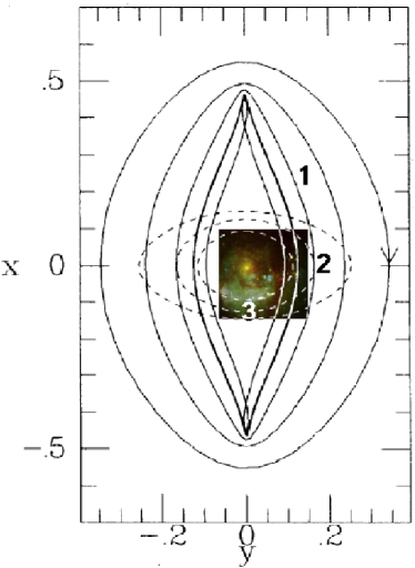
Figure 11: A fiducial illustration of $x_{1}$ orbits (solid lines) and $x_{2}$ orbits (broken lines) in a typical bar potential (actually for the Milky Way), adapted from Binney et al. (1991), with the false-colour image of Fig. 7 rotated and superimposed; the x-axis is aligned with the bar major axis while the y-axis is aligned with the bar minor axis. The bold line shows a ‘cusped’ $x_{1}$ orbit which separates the outer $x_{1}$ orbits from their smaller self-intersecting counterparts. Gas shocks along the leading edges of the bar and flows inwards to make the dust lane (at the point marked 1). This flow gradually funnels the gas onto suitable $x_{2}$ orbits at the point marked 2, although see Regan & Teuben (2003) and Maciejewski (2004) for complete hydrodynamical simulations. If there was a source of star formation at this point (as proposed in the models of Regan & Teuben), such as the partner dust lane merging at the same location, then the age gradient along the circumnuclear arc could just be a result of the young stars moving on $x_{2}$ orbits away from this location.

The CO maps of Sakamoto et al. (2004) clearly show the molecular hydrogen in both dust lanes joining in a ring like structure. The material from the southern dust lane appears to join the ring and move on the opposite side to the star burst arc to merge with the northern dustlane at the point where we see the youngest stars. Star formation at this point in the dust lane would usually be opposed because of the shear forces in action along the inevitable shocks; however, as in the simulations of Athanassoula (1992) and Maciejewski (2004), we observe the shock front (located by the gradient in $\textrm{V}_{\textrm{\scriptsize gas}}$) on the inner (southern) edge of the dust lane. On the outer edge, away from the shock front, where there is likely to be spurs and feathering (e.g. as found in Bonnell & Dobbs 2006) and less shear forces, star formation may be less opposed. For stars formed here, on the western edge of the dust lane, orbital motion dictates their trajectory and they will propagate along $x_{2}$ like orbits (illustrated in Fig. 11 and also Fig. 15 of Regan & Teuben 2003) to produce the ‘star forming’ arc. The gradient in age therefore reflects the older clusters having propagated further along their mutual $x_{2}$ orbits. However, it is not obvious why the youngest star clusters we observe are 4.5 Myrs old; one would expect them to be younger, unless the spraying of material as in Regan et al. (1999) led to star formation further up the dust lane. Equally, if star formation occurred on the opposite side to where we see the youngest clusters, triggered by the gas in the south-west of the ring merging with the south-west lane (the opposite of the previous scenario), then we would still expect an arc or ring of young stars to form but the timescales (dynamical and population synthesis) would agree better. If this were the case, we presumably do not see the young stars in the north of the ring due to the low luminosity of very young clusters ($<5$ Myrs) and the higher extinction there (seen in Fig. 10). Finally, there may be star formation at both sites: the newly formed stars would still propagate on the same $x_{2}$ orbits but the star formation from each point of contact does not need to be equal: the north-east dustlane appears denser in the CO data of Sakamoto et al. and could dominate the star formation. As previously discussed, we know that dual star formation events, separated by the dynamical timescale, can almost mimic a finite star formation episode of similar duration, but our attempts to fit such a model to the data were not as successfull as a single finite episode.

A nuclear spiral or ring would cause the young clusters in the arc to be rotating around the galaxy centre in the same manner: clockwise as we see them in Fig. 2 (assuming that the ring is co-planar with the galaxy). M83 is almost face on, so the rotation is difficult to detect, but the slight inclination (24^∘, Talbot et al., 1979) to our line-of-sight suggests that in the velocity data of T00, we can see stars on the south-west side of the nucleus (coincident with the young clusters) streaming away from us and the stars on the north-east side stream towards us, in agreement with an inclined clockwise rotation. However, this slit (labelled slit E in Fig. 3) mainly covers the background population rather than bright young clusters, so the velocity gradient could easily represent the overall rotation of the bulge. For consistency, let us estimate the dynamical time of the stars. From Fig. 10, we see that the average velocity of the stars either side of the nucleus (and at the position of the arc) is roughly constant at $\pm 25$km s^-1 in the rest frame of the galaxy nucleus along our line of sight. Assuming an inclination of 24^∘ then gives us an estimate for the circular velocity of 60km s^-1 $\sim 60$ pc $\textrm{Myr}^{-1}$ (also comparable to the average velocity dispersion). If the circumnuclear arc is around $15\arcsec\sim 260\textrm{pc}$ in circumference, we expect the stars to take around 4 Myrs to travel from one end to the other. This is in good agreement with the age decrement found by comparing the cluster ages on either end of the luminous arc ($\sim$3.5 Myrs). This point was also made in D06b, but the interpretation was significantly different. The dynamical timescale also changes with radius, which may help explain radial age gradients.

We note that the northen dust lane does not appear to follow the same route as the stars along the arc in the HST images but instead continues to propagate south, past the nucleus. This might appear be a concern for the above scenarios. However, the CO maps (Sakamoto et al., 2004) clearly show the majority of molecular hydrogen gas follows the outer edge of the circumnuclear arc. We also note that in the simulations of Piner et al. (1995), Regan et al. (1999) and Regan & Teuben (2003), similar features, where some gas appears to continue past the ring, can sometimes be seen, although they are very faint (not massive): in Regan et al. (1999) they are referred to as spray regions (also discussed by Sakamoto et al.) and in Maciejewski (2007) they are seen to be associated with regions of large shear.

6.3 The displaced nucleus

If the arc of young stars is a consequence of a nuclear spiral in the gas, we are left pondering why the only visible and kinematically detected nucleus at the centre of M83 is displaced from the centre of the galaxy and why we only see an arc of young stars rather than a ring. Apart from the arguments of Sofue & Wakamatsu (1994) who suggest that a complete ring is inclined to the galaxy disk and obscured on the northern side, one should also consider a natural m=1 mode. Although rare, M83 is not the only spiral galaxy to show central asymmetries: NGC 1672 is barred spiral with a nucleus displaced from the kinematic and bulge centre, as D06b highlight; NGC 3504 appears to show a single dominant spiral arm in H$\alpha$ and [NII] encompassing an offset nucleus (Emsellem, 2001); NGC 3227 and NGC 7130 are both spirals highlighted in Muñoz Marín et al. (2007) as having off-centred nuclei; NGC 1808 is another barred spiral with a circumnuclear starburst and nucleus offset from the kinematic centre (Tacconi-Garman et al., 1996, 2005) while NGC 4303 shows asymmetric star formation and dust lanes although the nucleus appears well centred (Schinnerer et al., 2002). Although some of these galaxies are clearly interacting, none have clearly merged to an extent where the nuclei are likely to have been accreted externally from the present interaction. Bournaud et al. (2005) have shown that m=1 modes in the outer regions of disk galaxies can be reproduced with a lopsided external accretion rather than a direct merger: if the outer regions of the galaxy are asymmetric, it may not be easy to define where the true morphological centre lies. That said, M83 does not look particularly disturbed or lopsided in the outer regions. If m=1 modes in the outer disk can be induced by an external accretion event, it may also be possible for m=1 modes to be induced by asymmetric accretion in the inner regions: in the CO maps of Sakamoto et al. (2004), it appears that the gas inflow in M83 is slightly asymmetric, with the north-eastern dust lane denser than the south-west lane at the point of contact to the circumnuclear CO ring; this might cause unequal forcing on any nuclear spiral, although hydrodynamical models are needed to confirm such a possibility. Finally, as noted by Sakamoto et al. (2004) the nucleus could be suffering a natural, unprovoked, instability as seen in the models of Taga & Iye (1998) or Lovelace et al. (1999) where the central nuclei are able to wander in the disk; such an instability might also be provoked by asymmetric inflow of gas. We noted earlier that the systematic velocity of the gas in the galaxy was taken to be 512 km s^-1 but in Fig. 10 the nucleus is moving towards us relative to this frame of reference at around 25km s^-1, so not only is the nucleus displaced from the centre of the bulge, it is also decoupled kinematically.

There is no evidence in the stellar kinematics of hidden mass concentrations at the locations previously proposed by T00 or D06(a,b). Without an integral field stellar velocity field of the central region of M83, we cannot completely rule out the presence of another hidden nucleus elsewhere, e.g. near the kinematical and bulge centre. However, given our extinction map (Fig. 4, from which we estimate $\textrm{A}_{\textrm{\scriptsize V}}$ $<3$ at the kinematic and bulge centre, corresponding to $\textrm{A}_{\textrm{\scriptsize K}}$$<0.3$), the NICMOS F222M photometry (Fig. 2), shows no massive luminous stellar feature other than the well known displaced nucleus: it is difficult to hide $10^{7}$$\textrm{M}_{\odot}$ of luminous stars with only 0.3 magnitudes of extinction.

7 Conclusion

We have shown that the NIR indices W[Pa$\alpha$] and W[CO] can be used to age-date young star clusters. Furthermore, W[Pa$\alpha$] is much less affected by extinction than W[H$\alpha$], which requires significant correction. The young clusters in the circumnuclear arc are inconsistent with simple stellar populations produced by an instantaneous burst; the observations require a finite episode of star formation lasting around 6 Myrs. Such models together with our observations provide the clearest evidence yet of an age gradient along the star forming arc, as first found in H01. However, our NIR observations further show that the circumnuclear arc does not stop at the edge of the dust lane, but continues through and along its north-west edge.

Our stellar kinematics show no evidence for a second obscured nucleus at either the location of D06b or T00 and we conclude that the velocity gradients in the gas kinematics (ionised and molecular) are a result of a shock front on the south-eastern edge of the north-eastern dust lane. We therefore explore alternative explanations for the formation of the circumnuclear arc, the most plausible being the $x_{2}$ orbital motion of the clusters from their place of birth in the dust lane.

Future higher-resolution integral field spectroscopy in the NIR has the potential to build on this study and find the youngest clusters in the arc (suspected to be on the north-west edge of the northern dust lane) and also address previous claims of an age gradient perpendicular to the arc (H01).

8 Acknowledgements

We wish to thank the referee for his/her constructive comments and Sabine Mengel for kindly providing the supergiant templates which we use when extracting the kinematics. We are also grateful for many fruitfull discussions with Witold Maciejewski and James Binney. We acknowledge that the linear sequence of radio sources proposed to be a background galaxy by Maddox et al. (2006) was discussed in a talk by Dottori et al. (2007, proceedings currently unpublished and no pre-print available) as a feature in the M83 disk possibly linked to the offset nucleus. This research is based on observations collected at the European Southern Observatory and the Hubble Space Telescope. We acknowledge use of the SIMBAD Astronomical Database, the HyperLeda database and NASA’s IDL Astronomy User’s Library. RH is funded by the University of Oxford and NT is funded through the Marie-Curie Excellence Grant MEXT-CT-2003-002792.

References

- Allard et al. (2006) Allard E. L., Knapen J. H., Peletier R. F., Sarzi M., 2006, MNRAS, 371, 1087
- Athanassoula (1992) Athanassoula E., 1992, MNRAS, 259, 345
- Baes et al. (2003) Baes M., Davies J. I., Dejonghe H., Sabatini S., Roberts S., Evans R., Linder S. M., Smith R. M., de Blok W. J. G., 2003, MNRAS, 343, 1081
- Binney et al. (1991) Binney J., Gerhard O. E., Stark A. A., Bally J., Uchida K. I., 1991, MNRAS, 252, 210
- Bonnell & Dobbs (2006) Bonnell I. A., Dobbs C. L., 2006, ArXiv Astrophysics e-prints
- Bournaud et al. (2005) Bournaud F., Combes F., Jog C. J., Puerari I., 2005, A&A, 438, 507
- Bresolin & Kennicutt (2002) Bresolin F., Kennicutt Jr. R. C., 2002, ApJ, 572, 838
- Buta (1986) Buta R., 1986, ApJS, 61, 609
- Buta & Combes (1996) Buta R., Combes F., 1996, Fundamentals of Cosmic Physics, 17, 95
- Calzetti (1997) Calzetti D., 1997, AJ, 113, 162
- Calzetti (2001) —, 2001, PASP, 113, 1449
- Calzetti et al. (2004) Calzetti D., Harris J., Gallagher III J. S., Smith D. A., Conselice C. J., Homeier N., Kewley L., 2004, AJ, 127, 1405
- Calzetti et al. (1994) Calzetti D., Kinney A. L., Storchi-Bergmann T., 1994, ApJ, 429, 582
- Cardelli et al. (1989) Cardelli J. A., Clayton G. C., Mathis J. S., 1989, ApJ, 345, 245
- Chung & Bureau (2004) Chung A., Bureau M., 2004, AJ, 127, 3192
- Combes (1996) Combes F., 1996, in Astronomical Society of the Pacific Conference Series, Vol. 91, IAU Colloq. 157: Barred Galaxies, Buta R., Crocker D. A., Elmegreen B. G., eds., pp. 286–+
- Cowan et al. (1994) Cowan J. J., Roberts D. A., Branch D., 1994, ApJ, 434, 128
- de Vaucouleurs et al. (1991) de Vaucouleurs G., de Vaucouleurs A., Corwin Jr. H. G., Buta R. J., Paturel G., Fouque P., 1991, Third Reference Catalogue of Bright Galaxies. Volume 1-3, XII, 2069 pp. 7 figs.. Springer-Verlag Berlin Heidelberg New York
- Diaz et al. (2007) Diaz R., Rodrigues I., Dottori H., Mast D., Agüero M. P., 2007, in IAU Symposium, Vol. 235, IAU Symposium, Combes F., Palous J., eds., pp. 93–93
- Díaz et al. (2006b) Díaz R. J., Dottori H., Aguero M. P., Mediavilla E., Rodrigues I., Mast D., 2006b, ApJ, 652, 1122
- Diaz et al. (2006a) Diaz R. J., Dottori H., Mediavilla E., Aguero M., Mast D., 2006a, New Astronomy Review, 49, 547
- Dottori et al. (2007) Dottori H., Diaz R. J., Aguero M. P., Mast D., Rodrigues I., 2007, in IAU Symposium, Vol. 245, IAU Symposium, in press, Bureau M., ed.
- Elmegreen et al. (1998) Elmegreen D. M., Chromey F. R., Warren A. R., 1998, AJ, 116, 2834
- Emsellem (2001) Emsellem E., 2001, in Astronomical Society of the Pacific Conference Series, Vol. 249, The Central Kiloparsec of Starbursts and AGN: The La Palma Connection, Knapen J. H., Beckman J. E., Shlosman I., Mahoney T. J., eds., pp. 91–+
- Emsellem et al. (2001) Emsellem E., Greusard D., Combes F., Friedli D., Leon S., Pécontal E., Wozniak H., 2001, A&A, 368, 52
- Escala et al. (2004) Escala A., Larson R. B., Coppi P. S., Mardones D., 2004, ApJ, 607, 765
- Fagotto et al. (1994) Fagotto F., Bressan A., Bertelli G., Chiosi C., 1994, A&AS, 105, 29
- Falcón-Barroso et al. (2007) Falcón-Barroso J., Boeker T., Schinnerer E., Knapen J. H., Ryder S., 2007, ArXiv e-prints, 709
- Förster Schreiber et al. (2003) Förster Schreiber N. M., Genzel R., Lutz D., Sternberg A., 2003, ApJ, 599, 193
- Gallais et al. (1991) Gallais P., Rouan D., Lacombe F., Tiphene D., Vauglin I., 1991, A&A, 243, 309
- Harris et al. (2001) Harris J., Calzetti D., Gallagher III J. S., Conselice C. J., Smith D. A., 2001, AJ, 122, 3046
- Heap et al. (1993) Heap S. R., Holbrook J., Malumuth E., Shore S., Waller W., 1993, in Bulletin of the American Astronomical Society, Vol. 25, Bulletin of the American Astronomical Society, pp. 840–+
- Hinkle et al. (2000) Hinkle K. H., Aringer B., Lebzelter T., Martin C. L., Ridgway S. T., 2000, A&A, 363, 1065
- Holtzman et al. (1995) Holtzman J. A., Hester J. J., Casertano S., Trauger J. T., Watson A. M., Ballester G. E., Burrows C. J., Clarke J. T., Crisp D., Evans R. W., Gallagher III J. S., Griffiths R. E., Hoessel J. G., Matthews L. D., Mould J. R., Scowen P. A., Stapelfeldt K. R., Westphal J. A., 1995, PASP, 107, 156
- Houghton et al. (2006) Houghton R. C. W., Magorrian J., Sarzi M., Thatte N., Davies R. L., Krajnović D., 2006, MNRAS, 367, 2
- Kenney et al. (1993) Kenney J. D. P., Carlstrom J. E., Young J. S., 1993, ApJ, 418, 687
- Kim & Kim (2007) Kim H., Kim W.-T., 2007, ApJ, 665, 432
- Kleinmann & Hall (1986) Kleinmann S. G., Hall D. N. B., 1986, ApJS, 62, 501
- Kobulnicky et al. (1999) Kobulnicky H. A., Kennicutt Jr. R. C., Pizagno J. L., 1999, ApJ, 514, 544
- Koribalski et al. (2004) Koribalski B. S., Staveley-Smith L., Kilborn V. A., Ryder S. D., Kraan-Korteweg R. C., Ryan-Weber E. V., Ekers R. D., Jerjen H., Henning P. A., Putman M. E., Zwaan M. A., de Blok W. J. G., Calabretta M. R., Disney M. J., Minchin R. F., Bhathal R., Boyce P. J., Drinkwater M. J., Freeman K. C., Gibson B. K., Green A. J., Haynes R. F., Juraszek S., Kesteven M. J., Knezek P. M., Mader S., Marquarding M., Meyer M., Mould J. R., Oosterloo T., O’Brien J., Price R. M., Sadler E. M., Schröder A., Stewart I. M., Stootman F., Waugh M., Warren B. E., Webster R. L., Wright A. E., 2004, AJ, 128, 16
- Kormendy & Richstone (1995) Kormendy J., Richstone D., 1995, ARA&A, 33, 581
- Krumholz et al. (2006) Krumholz M. R., Matzner C. D., McKee C. F., 2006, ApJ, 653, 361
- Larsen & Richtler (1999) Larsen S. S., Richtler T., 1999, A&A, 345, 59
- Leitherer & Heckman (1995) Leitherer C., Heckman T. M., 1995, ApJS, 96, 9
- Leitherer et al. (1999) Leitherer C., Schaerer D., Goldader J. D., Delgado R. M. G., Robert C., Kune D. F., de Mello D. F., Devost D., Heckman T. M., 1999, ApJS, 123, 3
- Lovelace et al. (1999) Lovelace R. V. E., Zhang L., Kornreich D. A., Haynes M. P., 1999, ApJ, 524, 634
- Maciejewski (2004) Maciejewski W., 2004, MNRAS, 354, 892
- Maciejewski (2007) —, 2007, ArXiv e-prints, 709
- Maddox et al. (2006) Maddox L. A., Cowan J. J., Kilgard R. E., Lacey C. K., Prestwich A. H., Stockdale C. J., Wolfing E., 2006, AJ, 132, 310
- Malin & Hadley (1997) Malin D., Hadley B., 1997, Publications of the Astronomical Society of Australia, 14, 52
- Martini & Pogge (1999) Martini P., Pogge R. W., 1999, AJ, 118, 2646
- Mast et al. (2006) Mast D., Díaz R. J., Agüero M. P., 2006, AJ, 131, 1394
- Meynet et al. (1994) Meynet G., Maeder A., Schaller G., Schaerer D., Charbonnel C., 1994, A&AS, 103, 97
- Miller & Bregman (2005) Miller E. D., Bregman J. N., 2005, in Astronomical Society of the Pacific Conference Series, Vol. 331, Extra-Planar Gas, Braun R., ed., pp. 261–+
- Muñoz Marín et al. (2007) Muñoz Marín V. M., González Delgado R. M., Schmitt H. R., Cid Fernandes R., Pérez E., Storchi-Bergmann T., Heckman T., Leitherer C., 2007, AJ, 134, 648
- Oliva et al. (1995) Oliva E., Origlia L., Kotilainen J. K., Moorwood A. F. M., 1995, A&A, 301, 55
- Origlia et al. (1999) Origlia L., Goldader J. D., Leitherer C., Schaerer D., Oliva E., 1999, ApJ, 514, 96
- Origlia et al. (1993) Origlia L., Moorwood A. F. M., Oliva E., 1993, A&A, 280, 536
- Osterbrock (1989) Osterbrock D. E., 1989, Astrophysics of gaseous nebulae and active galactic nuclei. Research supported by the University of California, John Simon Guggenheim Memorial Foundation, University of Minnesota, et al. Mill Valley, CA, University Science Books, 1989, 422 p.
- Ostriker (1999) Ostriker E. C., 1999, ApJ, 513, 252
- Park et al. (2001) Park O.-K., Kalnajs A., Freeman K. C., Koribalski B., Staveley-Smith L., Malin D. F., 2001, in Astronomical Society of the Pacific Conference Series, Vol. 230, Galaxy Disks and Disk Galaxies, Funes J. G., Corsini E. M., eds., pp. 109–110
- Piner et al. (1995) Piner B. G., Stone J. M., Teuben P. J., 1995, ApJ, 449, 508
- Pogge & Martini (2002) Pogge R. W., Martini P., 2002, ApJ, 569, 624
- Puxley et al. (1997) Puxley P. J., Doyon R., Ward M. J., 1997, ApJ, 476, 120
- Regan et al. (1999) Regan M. W., Sheth K., Vogel S. N., 1999, ApJ, 526, 97
- Regan & Teuben (2003) Regan M. W., Teuben P., 2003, ApJ, 582, 723
- Rix & White (1992) Rix H.-W., White S. D. M., 1992, MNRAS, 254, 389
- Rogstad et al. (1974) Rogstad D. H., Lockart I. A., Wright M. C. H., 1974, ApJ, 193, 309
- Ryder et al. (2005) Ryder S. D., Sharp R. G., Knapen J. H., Mazzuca L. M., Parry I. R., 2005, in American Institute of Physics Conference Series, Vol. 783, The Evolution of Starbursts, Hüttmeister S., Manthey E., Bomans D., Weis K., eds., pp. 155–160
- Sakamoto et al. (2004) Sakamoto K., Matsushita S., Peck A. B., Wiedner M. C., Iono D., 2004, ApJ, 616, L59
- Sandage & Bedke (1994) Sandage A., Bedke J., 1994, The Carnegie atlas of galaxies. Washington, DC: Carnegie Institution of Washington with The Flintridge Foundation, —c1994
- Sarazin & Roddier (1990) Sarazin M., Roddier F., 1990, A&A, 227, 294
- Sarzi et al. (2007) Sarzi M., Allard E. L., Knapen J. H., Mazzuca L. M., 2007, MNRAS, 380, 949
- Sarzi et al. (2006) Sarzi M., Falcón-Barroso J., Davies R. L., Bacon R., Bureau M., Cappellari M., de Zeeuw P. T., Emsellem E., Fathi K., Krajnović D., Kuntschner H., McDermid R. M., Peletier R. F., 2006, MNRAS, 366, 1151
- Schinnerer et al. (2002) Schinnerer E., Maciejewski W., Scoville N., Moustakas L. A., 2002, ApJ, 575, 826
- Sofue & Wakamatsu (1994) Sofue Y., Wakamatsu K.-I., 1994, AJ, 107, 1018
- Soria & Wu (2003) Soria R., Wu K., 2003, A&A, 410, 53
- Storchi-Bergmann et al. (1995) Storchi-Bergmann T., Kinney A. L., Challis P., 1995, ApJS, 98, 103
- Tacconi-Garman et al. (1996) Tacconi-Garman L. E., Sternberg A., Eckart A., 1996, AJ, 112, 918
- Tacconi-Garman et al. (2005) Tacconi-Garman L. E., Sturm E., Lehnert M., Lutz D., Davies R. I., Moorwood A. F. M., 2005, A&A, 432, 91
- Taga & Iye (1998) Taga M., Iye M., 1998, MNRAS, 299, 1132
- Talbot et al. (1979) Talbot Jr. R. J., Jensen E. B., Dufour R. J., 1979, ApJ, 229, 91
- Thatte et al. (2000) Thatte N., Tecza M., Genzel R., 2000, A&A, 364, L47
- Thilker et al. (2005) Thilker D. A., Bianchi L., Boissier S., Gil de Paz A., Madore B. F., Martin D. C., Meurer G. R., Neff S. G., Rich R. M., Schiminovich D., Seibert M., Wyder T. K., Barlow T. A., Byun Y.-I., Donas J., Forster K., Friedman P. G., Heckman T. M., Jelinsky P. N., Lee Y.-W., Malina R. F., Milliard B., Morrissey P., Siegmund O. H. W., Small T., Szalay A. S., Welsh B. Y., 2005, ApJ, 619, L79
- Thim et al. (2003) Thim F., Tammann G. A., Saha A., Dolphin A., Sandage A., Tolstoy E., Labhardt L., 2003, ApJ, 590, 256
- Vázquez & Leitherer (2005) Vázquez G. A., Leitherer C., 2005, ApJ, 621, 695
- Wolstencroft (1988) Wolstencroft R. ., 1988, in Proceedings of a Conference, held in honor of the 60th birthday of Halton C. Arp, Venice, Italy, May 5-7, 1987, Cambridge: University Press, 1988, edited by Bertola, F.; Sulentic, J.W.; Madore, B.F., Bertola F., Sulentic J., Madore B., eds.
- Wozniak & Champavert (2006) Wozniak H., Champavert N., 2006, MNRAS, 369, 853
- Wozniak et al. (2003) Wozniak H., Combes F., Emsellem E., Friedli D., 2003, A&A, 409, 469