Heterogeneous bounds of confidence: Meet, Discuss and Find Consensus!

Abstract

Models of continuous opinion dynamics under bounded confidence show a sharp transition between a consensus and a polarization phase at a critical global bound of confidence. In this paper, heterogeneous bounds of confidence are studied. The surprising result is that a society of agents with two different bounds of confidence (open-minded and closed-minded agents) can find consensus even when both bounds of confidence are significantly below the critical bound of confidence of a homogeneous society.

The phenomenon is shown by examples of agent-based simulation and by numerical computation of the time evolution of the agents density. The result holds for the bounded confidence model of Deffuant, Weisbuch and others (Weisbuch, G. et al; Meet, discuss, and segregate!, Complexity, 2002, 7, 55–63), as well as for the model of Hegselmann and Krause (Hegselmann, R., Krause, U.; Opinion Dynamics and Bounded Confidence, Models, Analysis and Simulation, Journal of Artificial Societies and Social Simulation, 2002, 5, 2).

Thus, given an average level of confidence, diversity of bounds of confidence enhances the chances for consensus. The drawback of this enhancement is that opinion dynamics becomes suspect to severe drifts of clusters, where open-minded agents can pull closed-minded agents towards another cluster of closed-minded agents. A final consensus might thus not lie in the center of the opinion interval as it happens for uniform initial opinion distributions under homogeneous bounds of confidence. It can be located at extremal locations. This is demonstrated by example.

This also show that the extension to heterogeneous bounds of confidence enriches the complexity of the dynamics tremendously.

1 Introduction

Reaching consensus about certain issues is often desired in a society. In which society are the chances for consensus better? A society with homogeneous agents which are equally skeptical about the opinions of others or a heterogeneous society with open- and closed-minded people? We study this question in the framework of continuous opinion dynamics under bounded confidence. The surprising result is that very often a heterogeneous society can reach consensus even when both open-minded and closed-minded agents are more skeptical than in a homogeneous society.

Models of continuous opinion dynamics under bounded confidence have been introduced independently by Hegselmann and Krause (HK) Krause.Stockler1997ModellierungundSimulation ; Krause2000DiscreteNonlinearand ; Hegselmann.Krause2002OpinionDynamicsand and Deffuant, Weisbuch and others (DW) Deffuant.Neau.ea2000MixingBeliefsamong ; Weisbuch.Deffuant.ea2002Meetdiscussand . In the basic version of both models agents adjust their continuous-value opinions toward the opinions of other agents, but they only take opinions of others into account if they are closer than a bound of confidence $\varepsilon$ to their own opinion. The DW and the HK model differ in their communication regime. In the DW model agents meet in random pairwise encounters. In the HK model update is synchronous and each agent takes into account only other agents within bounds of confidence around her current opinion. Both models extend naturally to heterogeneous bounds of confidence. But the case has only been briefly addressed in Weisbuch.Deffuant.ea2002Meetdiscussand and in Groeber.Schweitzer.ea2009HowGroupsCan under further extensions to the network of past interactions.

Opinion dynamics starts with an ensemble of $n$ agents with initial opinions in the interval $[0,1]$. Dynamics always lead to a stable configuration where opinions form opinion clusters (see Lorenz2005stabilizationtheoremdynamics for a proof). If there is only one final cluster the agents have reached consensus. But there are also other characteristic cluster configurations with respect to number, sizes and locations of opinion clusters. The configuration reached is mostly determined by the bound of confidence $\varepsilon$. Of course, the final configuration depends also on the specific initial opinions and in the DW model on the specific realization for the pairwise encounters. But these parameters are regarded as random and equally distributed in this paper and in most of the existing literature (with the exception of Lorenz.Urbig2007AboutPowerto ). Both models are invariant to joint shifts and scales of the initial configuration and the bound of confidence. Thus, the restriction to the opinion interval $[0,1]$ gives still a full characterization of model dynamics on bounded intervals.

The simulations of the models show a sharp transition between a consensus phase and a polarization phase at a critical bound of confidence. Polarization is meant to be a final state with two equally sized big clusters while consensus is meant to be a final state where one big cluster is dominant, usually located in the center of the opinion space.

The behavioral rules of agent-based models can be taken over to density-based models where dynamics are defined on the density of agents in the opinion space. This reformulation allows a better estimate of the critical values for the bound of confidence Ben-Naim.Krapivsky.ea2003BifurcationandPatterns ; Fortunato.Latora.ea2005VectorOpinionDynamics ; Lorenz2007ContinuousOpinionDynamics . The approach also extends naturally to heterogeneous bounds of confidence.

In Section 2 the formal definition of the agent-based DW and HK model with heterogeneous bounds of confidence is given and the phenomenon of consensus for low bounds of confidence is demonstrated by examples. In this paper we only treat two different bounds of confidence, because this already improves the complexity of the dynamical behavior significantly. Further on, the density based approach is introduced and demonstrated by examples. In Section 3 the density-based approach is used to systematically study the evolving cluster patterns under uniform initial conditions. Section 4 demonstrates the phenomenon of drifting towards extremes by example. Drifting appear even for slight unstructured perturbations of the uniform distribution. It is shown by agent-based as well as density-based examples. Section 5 gives conclusions.

2 DW and HK model extended to heterogeneous bounds of confidence

In the following we give the definition of both bounded confidence models including their natural extension to heterogeneous bounds of confidence.

Let us consider $n$ agents which hold real numbers between zero and one as opinions. The opinion of agent $i$ at time $t$ is represented by $x_{i}(t)$ and $x(t)$ is the vector of opinions of all agents at time $t$ called the opinion profile. Suppose further on, that agent $i$ has a bound of confidence $\varepsilon_{i}$ which determines that she takes all agents as serious which differ not more than $\varepsilon_{i}$ from her opinion. Given an opinion profile $x(t)$ agent $i$ has the following confidence set $I_{\varepsilon_{i}}(i,x(t))=\{j\,|\,\left\|x_{i}(t)-x_{j}(t)\right\|\leq\varepsilon_{i}\}$. The confidence set of agent $i$ contains all agents whose opinions lie in the $2\varepsilon$-interval around $x_{i}(t)$. Naturally this includes the agent herself. Agent $i$ with opinion $x_{i}(t)$ is willing to adjust her opinion towards the opinions of others in her confidence set by building an arithmetic mean.

These definitions hold for both models. The differences of the DW and the HK model comes with the definition of who communicated with whom at what time.

In the DW model two agents $i,j$ are chosen randomly. Each agent changes her opinion to the average of both opinions if the other agent is in her confidence set. So

$$x_{i}(t+1)=\begin{cases}\frac{x_{i}(t)+x_{j}(t)}{2}&\textrm{if $j\in I_{\varepsilon_{i}}(i,t)$}\\ x_{i}(t)&\textrm{otherwise.}\end{cases}$$

The same for $x_{j}(t+1)$ with $i$ and $j$ interchanged.

It is important to notice, that it is well possible that one agent with high bound of confidence changes her opinion, while the other with low bound of confidence does not. The convergence parameter $\mu$ of the original model Deffuant.Neau.ea2000MixingBeliefsamong ; Weisbuch.Deffuant.ea2002Meetdiscussand is neglected to not further increase the complexity. In Deffuant.Neau.ea2000MixingBeliefsamong ; Weisbuch.Deffuant.ea2002Meetdiscussand it has been argued that $\mu$ effects only convergence time, later it has been shown that the parameter also impacts the sizes of minority clusters Laguna.Abramson.ea2004Minoritiesinmodel or might get very important under other extensions Lorenz.Urbig2007AboutPowerto .

Figure 1 shows an example for the DW model in which 500 of 1000 agents are closed-minded ($\varepsilon_{1}=0.11$), the other half open-minded ($\varepsilon_{2}=0.22$). Both bounds are far less than $\varepsilon_{\text{crit}}\approx 0.27$ which is the critical bound for the consensus transition in the homogeneous DW model (see Lorenz2007ContinuousOpinionDynamics ). The figure shows the characteristic patterns with four respectively two big final clusters evolving in the cases with homogeneous $\varepsilon_{1}$ respectively $\varepsilon_{2}$. The main plot shows how consensus (neglecting small extremal clusters) is achieved when bounds of confidence are mixed. This is the central phenomenon this paper is about.

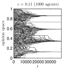
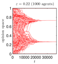
Figure 1: DW processes with 1000 agents. Closed minded agents are black, open-minded are (red). Initial conditions in all runs are equal. It is possible for the agents to reach consensus under heterogeneous bounds of confidence (bottom) but not in the corresponding homogeneous cases (top).

In the HK model all agents act at the same time, and each changes her opinion to the average of the opinions of all agents in her confidence set. So,

$$x_{i}(t+1)=\frac{1}{\#I_{\varepsilon_{i}}(i,x(t))}\sum_{j\in I_{\varepsilon_{i}}(i,x(t))}x_{j}(t)$$

for all $i$. ($\#$ is the number of elements of a set.) Figure 2 shows an example for the HK model. Because of the higher computational effort a small system of 150 closed-minded ($\varepsilon_{1}=0.11$) and 150 open-minded ($\varepsilon_{2}=0.19$) is chosen. For the HK model the critical bound of confidence for the consensus transition lies at about $\varepsilon=0.19$ (see Lorenz2007ContinuousOpinionDynamics ), but this result is achieved using the density based approach and it turns out by simulation that consensus in the region of 0.19 is only achieved for very large and very uniform distributed intital conditions. Thus, Figure 2 is another example where consensus is never achieved in the homogeneous models (with system sizes of $n=300$), while mixing can lead to consensus.

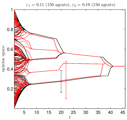
Figure 2: HK processes with 300 agents. Closed minded agents are black, open-minded are (red). Initial conditions in all runs are equal. Initial conditions in all runs are equal. It is possible for the agents to reach consensus under heterogeneous bounds of confidence (bottom) but not in the corresponding homogeneous cases (top).

A great success in understanding dynamics of these models was possible through the introduction of density-based reformulations Ben-Naim.Krapivsky.ea2003BifurcationandPatterns of the DW model. The basic idea is to define dynamics on the space of density functions with the opinion interval as the domain and use the same heuristics as in the agent-based models. So, the scope changes from a finite number of agents to an idealized infinite number of agents which are distributed in the opinion interval as defined by the density function. (In Blondel.Hendrickx.ea20072Rconjecturemulti-agent another model with an infinite number of agents is introduced which allows to transform agent-based dynamics more straight forward. The density-based approach can be derived from that.) This way, the evolution of the agent density in the opinion interval can be computed numerically for any initial opinion density. This allows to get an overview about the average behavior of agent-based dynamics by computing numerically just one evolution of the agent density in the opinion interval. The density-based computation matches agent-based fairly well when the number of agents is sufficiently large and the initial agent-based opinion profile is a proper draw from the initial agent distribution in the density-based model. Thus, this approach avoids noisy Monte-Carlo simulations and gives a good overview on attractive states. The density-based approach has been used to derive bifurcation diagrams for the evolving cluster patterns with respect to a homogeneous bound of confidence for the initial opinion distributions to be uniform in the opinion space.

For the HK model the same approach was first applied independently in Fortunato.Latora.ea2005VectorOpinionDynamics and Lorenz2005Continuousopiniondynamics , for an overview and discussion of different methods see Lorenz2007ContinuousOpinionDynamics .

Density-based models have been proposed in continuous time and continuous opinion space Ben-Naim.Krapivsky.ea2003BifurcationandPatterns ; Fortunato.Latora.ea2005VectorOpinionDynamics as well as in discrete time and opinion space Lorenz2005Continuousopiniondynamics ; Lorenz2006Consensusstrikesback ; Lorenz2007RepeatedAveragingand . The discrete version takes the form of an interactive Markov chain, where transition probabilities depend on the current state of the system. For numerical computation the continuous opinion interval as well as time has to be discretized anyway. Therefore, we take the discrete approach directly in this paper.

The density-based models with homogeneous bounds of confidence can be extended for heterogeneous bounds of confidence straight forward by introducing a density function for each bound of confidence. The precise definition follows for simplicity for just two bounds of confidence $\varepsilon_{1}$ and $\varepsilon_{2}$. This setting is what we simulate systematically in the next section. The definition can be easily extended to more bounds of confidence and even a continuum of bounds of confidence.

Instead of agents and their opinions we define the state of the system as a density function on the opinion interval which evolves in time. We discretize the opinion space $[0,1]$ into $n$ subintervals $[0,\frac{1}{n}[,[\frac{1}{n},\frac{2}{n}[,\dots,[\frac{n-1}{n},1]$ which serve as opinion classes. So, we switch from $n$ agents with opinions in the opinion interval to an idealized infinite population, which is divided into $n$ opinion classes. We label opinion classes with $\{1,\dots,n\}$ such that class $1\leq i\leq n$ stands for opinions in the interval $[\frac{i-1}{n},\frac{i}{n}[$. The two bounds of confidence $\varepsilon_{1}$ and $\varepsilon_{2}$ naturally transform with respect to the $n$ opinion classes to their discrete counter-parts $\epsilon_{1}=n\varepsilon_{1}$ and $\epsilon_{2}=n\varepsilon_{2}$.

The state of the system is quantified by two row vectors $p^{1}(t),p^{2}(t)\in\mathbb{R}^{n}_{\geq 0}$, where $p_{i}^{k}(t)$ is the fraction of the total population which holds opinions in class $i$, have a bound of confidence $\epsilon_{k}$ at time $t$. The pair $(p^{1}(t),p^{2}(t))$ is called the opinion distribution at time $t$. One can see each vector $p^{k}$ as the histogram of the agents with bound of confidence $\epsilon_{k}$ over the opinion classes. Naturally, it should hold that the fractions sum up to one $\sum_{i,k}p^{k}_{i}(t)=1$. Further on, we define $p(t)=p^{1}(t)+p^{2}(t)$ to be the opinion distribution of the full population regardless of the bounds of confidence. We choose row vectors $p^{k}$ because this is a convention in defining discrete Markov chains. A discrete Markov chain is given by its transition matrix $T$ where $T_{ij}$ is the probability that an agent switches from state $i$ to $j$. Given a distribution $p(t)$ the next time step’s distribution is thus computed by $p(t+1)=p(t)T$. In our case the transition matrices will be a function of the current state. This is called an interactive Markov chain.

We consider that agents never change their bound of confidence. Therefore, we can define a transition matrix for the agents with discrete bound of confidence $\epsilon_{k}$ as $T(p(t),\epsilon_{k})$. Notice that the transition matrix depends on the opinion vector for the full population $p(t)=p^{1}(t)+p^{2}(t)$ only. This reflects, that the change of opinion of an agent with bound of confidence $\epsilon_{k}$ does not depend on the bounds of confidence of the other agents, only on the distribution of opinions in total and its own bound of confidence. The density-based dynamics is then defined for the initial distributions $(p^{1}(0),p^{2}(0))$ as

$$p^{1}(t+1)=p^{1}(t)T(p(t),\epsilon_{1})$$ (1)

$$p^{2}(t+1)=p^{2}(t)T(p(t),\epsilon_{2}).$$ (2)

This framework is applied for both models. So, we have to specify the transition matrices for the two models now.

The Deffuant-Weisbuch transition matrix is defined by

$$T^{\mathrm{DW}}_{ij}(p,\epsilon)=\left\{\begin{array}[]{ll}\frac{\pi^{i}_{2j-i-1}}{2}+\pi^{i}_{2j-i}+\frac{\pi^{i}_{2j-i+1}}{2},&\hbox{if $i\neq j$, }\\ q_{i},&\hbox{if $i=j$.}\\ \end{array}\right.$$

with $q_{i}=1-\sum_{j\neq i,j=1}^{n}T^{\mathrm{DW}}_{ij}(p,\epsilon)_{ij}$ and

$$\pi^{i}_{m}=\left\{\begin{array}[]{ll}p_{m},&\hbox{if $|i-m|\leq\epsilon$}\\ 0,&\hbox{otherwise}\\ \end{array}\right.$$

For $i<1$ and $i>n$ it is defined $p^{k}_{i}=0$ for convenience. The probability of an agent to change from opinion $i$ to opinion $j$ depends on the fractions of agents in the opinion classes $2j-i-1,2j-i,2j_{i}+1$, but only when these classes are not farther than $\epsilon_{i}$ from $i$. The average of $i$ and $2j-i$ is indeed $j$. The average of $i$ and $2j-i-1$ i s $j-\frac{1}{2}$, thus only half of the agents is expected to switch to state $j$ (the other half will switch to state $j-1$). Analog for averaging $i$ and $2j-i+1$.

Figure 3 shows an example computation for the evolution of an opinion distribution in the DW model. The distributions of the open-minded population (red) and the closed-minded (black) population are stacked to give an impression of the evolution of the whole population. Computations where carried out with 100 opinion classes, but runs would look essentially identically for a higher number of classes and an appropriate scaling of the discrete bounds of confidence. The example is with the same parameters as the agent-based example in Figure 1, and indeed shows the same phenomenon of convergence to a big central consensual cluster due to the interplay of closed and open-minded agents. Both groups play its role in reaching consensus. The closed-minded ensure that intermediately ($t=50$) there is a small cluster in the center of the opinion space. Open-minded agents at the same location would already been absorbed by the two big intermediate clusters on the right and on the left. Finally, the open-minded play their role in pulling the closed-minded from both sides slowly towards the center.

Figure 3: A density-based DW process with closed minded (black) and open-minded (red) agents. Time proceeds downwards. Notice that time steps are not equidistant, but selected to show important changes. The right hand side is just another scale of the y-axis which makes small classes visible. Values of bounds of confidence coincide Figure 1. Also a consensus is found (neglecting a small proportion of extremists).

The HK transition matrix is defined by

$$T^{\mathrm{HK}}_{ij}(p,\epsilon)=\left\{\begin{array}[]{ll}1&\hbox{if $j=M_{i}$,}\\ \lceil M_{i}\rceil-M_{i}&\hbox{if $j=\lfloor M_{i}\rfloor$, $j\neq M_{i}$,}\\ M_{i}-\lfloor M_{i}\rfloor&\hbox{if $j=\lceil M_{i}\rceil$, $j\neq M_{i}$,}\\ 0&\hbox{otherwise.}\\ \end{array}\right.$$

with

$$M_{i}(p,\epsilon)=\frac{\sum_{k=i-\epsilon}^{i+\epsilon}kp_{k}}{\sum_{k=i-\epsilon}^{i+\epsilon}p_{k}}$$

being the $\epsilon$-local mean at opinion class $i$. The brackets $\lfloor\cdot\rfloor$ represents rounding to the upper integer, $\lfloor\cdot\rfloor$ rounding to the lower integer. The $\epsilon$-local mean is the barycenter of distribution $p$ on the discrete interval of length $2\epsilon$ centered on opinion $i$. So, an agent switches from opinion $i$ to $j$ when $j$ is the $\epsilon$-local mean of $i$. If the $\epsilon$-local mean is not an integer it switches to the class above or below with probabilities depending on the distance of the $\epsilon$-local mean to these classes.

Figure 4 shows an example computation for the evolution of an opinion distribution in the HK model, which is in the same style of presentation as Figure 3 and matches the parameters of Figure 4. Again, consensus is found only due to the interplay of the closed- and the open-minded. A remark on comparison to the bifurcation diagram for the HK model reported in Lorenz2007ContinuousOpinionDynamics which gives $0.19$ as the critical value of the consensus transition. But consensus in this region is only achieved under very long convergence time and only for a large number of classes, there 1000, which corresponds to a very large number of agents in the agent-based version. So, consensus is possible in very large homogeneous groups under $\varepsilon=0.19$ by very long convergence times. In the example of Figure 4 consensus is achieved very fast under the heterogeneous bounds of confidence.

Figure 4: A density-based HK process with closed minded (black) and open-minded (red) agents. Time proceeds downwards. Notice that time steps are not equidistant, but selected to show important changes. The right hand side is just another scale of the y-axis which makes small classes visible. Values of bounds of confidence coincide Figure 2. Also a consensus is found.

The discrete time and discrete opinion space approach for density-based models presented here and the continuous approaches (DW Ben-Naim.Krapivsky.ea2003BifurcationandPatterns , HK Fortunato.Latora.ea2005VectorOpinionDynamics ) for density-based models have been shown to lead to the same results for the DW model Lorenz2007RepeatedAveragingand . This does not hold for the HK model (see Lorenz2007ContinuousOpinionDynamics for a discussion). Further on, it matters for the HK model if the discretization of the opinion interval is into an even or odd number of bins (see Lorenz2005Continuousopiniondynamics for evidence). In the following section we focus on odd numbers. Thus on distributions where a central bin exists which is the natural candidate for a consensus under a symmetric initial distribution. In the following section we will show by systematic simulations that the phenomenon of reaching consensus with lower but heterogeneous bounds of confidence is generic in the both models.

3 Systematic Simulation

In this section a complete picture is given about the final ‘degree of consensus’ for societies of closed- and open-minded agents which initial opinions are uniformly distributed in the opinion interval. Only the case of equally sized groups of closed- and open-minded agents is treated.

For a systematic simulation setup, the opinion space $[0,1]$ is divided into $n=201$ opinion classes. The initial opinion distribution is $p^{k}_{i}=\tfrac{1}{402}$ for $k=1,2$ and $i=1,\dots,n$. Then the final opinion distribution is computed for $\epsilon_{1},\epsilon_{2}=10,11,\dots,70$ which corresponds to $\varepsilon_{1},\varepsilon_{2}=\frac{10}{201},\dots,\frac{70}{201}\approx 0.05,\dots,0.35$. Notice that a formal proof for convergence to a stable opinion distribution is still lacking, see Lorenz2007ContinuousOpinionDynamics for discussion. For our setting convergence is evident by observation, but stopping criteria for simulation runs are difficult to define, especially for the DW model. For the HK model new time steps were computed until the difference to the former time steps got zero (due to computer precision limits). Convergence was achieved in reasonable time. Numerical problems evolved when distributions got asymmetric around the central class 101 for the reason of floating point errors. These problems were circumvented by making the opinion distributions symmetric again after each iteration. For the heterogeneous DW model stopping criteria are more complicated because it has a rich variety of types of convergence which are not fully classified and understood until now. Further on, convergence can last very long and it is difficult to decide whether convergence will lead to another drastic change once or not. Therefore, three different ways to visualize the results are chosen in Figure 5.

To quantify the ‘degree of consensus’ the mass of the biggest cluster is an appropriate measure. In a stabilized final opinion distribution a cluster is a set of at most two adjacent classes with positive mass surrounded by classes with zero mass (see Lorenz2007RepeatedAveragingand ; Lorenz2007Fixedpointsin ). Due to the odd number of classes and symmetry a cluster including the central class $i=101$ can finally only be a one-class cluster. The central class $i=101$ is also the only candidate where $p^{1}_{i}+p^{2}_{i}>0.5$ is possible due to conservation of symmetry. Convergence in the DW model is slow. This, concerns especially the final condensing to clusters, even when the broad separation into clusters has settled. Further on, masses remain always positive (though small). Thus, we have to come up with a cluster definition which we can apply in not fully converged situations. So we define an opinion cluster with precision $10^{-4}$ to be a set of adjacent opinion classes which all contain mass larger than $10^{-4}$ and which neighbor classes have mass less than $10^{-4}$.

The masses of the biggest cluster are documented in Figure 5 for the DW model and in Figure 6 for the HK model. We color the plane of all $(\varepsilon_{1},\varepsilon_{2})$ points with the values of the mass of the biggest cluster after stabilization. So, regions of certain degrees of consensus are dark red, while regions of almost consensual clusters are orange and red. Several abrupt and continuous transitions in changes of $\varepsilon_{1},\varepsilon_{2}$ are visible.

Figure 5: Mass of the biggest cluster with precision $10^{-4}$ after stabilization for the DW model (top). Mass of the largest class at time step $t=200$ (bottom left), and the time step $t$ when the mass of the central cluster exceeds 50% (blue stands for ‘never’).

Figure 6: Mass of the biggest cluster after stabilization for HK model.

Let us first take a look on the diagonal of the plots which represents the homogeneous situation $\varepsilon_{1}=\varepsilon_{2}$. We see the points of the consensus transition as about $0.27$ for the DW model and about $0.19$ for the HK model. (It can also be observed that consensus strikes back for $0.17$ in the HK model. See Lorenz2006Consensusstrikesback for details about this phenomenon.) The surprise comes when we look on the heterogeneous situations besides the diagonal. Consensus is in many cases possible even when $\varepsilon_{1}$ and $\varepsilon_{2}$ are both below the critical $\varepsilon$ for the consensus transition in the homogeneous case.

The evolution of consensus under heterogeneous bounds of confidence in the DW model looks quite ubiquitous. But it is important to notice that the plot for the DW model might look very different for different levels of precision. Further on, convergence time to consensus could be very slow. To clarify the picture about the DW model the two smaller plots are included in Figure 5. The bottom left plot shows the situation after a not so long time $t=200$. Because clusters can not be determined at this level we simply plot the maximum of $p_{i}(200)$ all opinion classes $i\in\{1,\dots,n\}$. One can see that especially in the region around $(\varepsilon_{1},\varepsilon_{2})=(0.11,0.22)$ the maximum has already exceeded $50\%$. So, in this region consensus will appear after a reasonable amount of time. The bottom right plot shows the time steps when the central class contains more than $50\%$ of the mass (if this happens at all). So, this is another measure for convergence to consensus in a reasonable time. The color axis has been adjusted from zero to thousand. For the blue area the central cluster has not exceeded $50\%$ either because of convergence to polarization or plurality (in the region around the diagonal) or because of too slow convergence (in the region at the corners). So, black stands for a huge time interval. The nonconverged states in the upper left and bottom right corner did not converged after $45.000$ time steps. Further on, there is one interesting example for long convergence time on the diagonal (the homogeneous case). This is an example for a very short $\varepsilon$-phase where convergence to consensus in the DW model is via a metastable polarized state, which has not been observed before. This slow convergence $\varepsilon$-phase close to the transition is really huge for the HK model (see Lorenz2006Consensusstrikesback ).

We can conclude that enhancement of the chances for consensus due to heterogeneity is generic. It appears due to a subtle interplay between closed- and open-minded agents. The results presented were all produced for initial opinion distributions which were perfectly uniform. In the following section we will study perturbations of this situation.

4 Inherent drifting towards the extremes

In the following it is demonstarted by example that even unstructured deviations from the perfect symmetry in the initial opinion distribution can have important consequences. Let us start by looking on some other agent-based examples. Figure 7 shows two different runs The upper plot shows a simulation run for the same initial conditions as Figure 1 but with a different realization of the pairwise encounters. Consensus is not achieved but a polarization into two big clusters. Moreover, both cluster drift towards zero. This happens in both big clusters due to their contact to a very small group of closed-minded agents which lies below each of them. This situation was achieved in the first 10000 time steps by the upper group moving slightly faster towards the center and thus attracting more of the closed-minded agents in the center. This brought the emerging big lower cluster to be more oriented to the even lower small cluster of closed minded. This established the situation of the overall drift to one side. Notice that this situation was not put a priori in, but emerged from a uniform distribution of open-minded as well as closed-minded agents. The bottom plot in Figure 7 shows an example with different parameters, which leads to an extremal consensus close to one. Again the initial configuration is unstructured. This shows that the system becomes suspect to extremism even when this susceptibility is not visible a priori. Extremism in bounded confidence models has already been studied Deffuant.Neau.ea2002HowCanExtremism ; Amblard.Deffuant2004roleofnetwork ; Deffuant2006ComparingExtremismPropagation , but in all of these studies the susceptibility to extremism was put in a priori by populating the extremes with very closed-minded agents, such that they form natural attractors for the open-minded central agents. The question in these studies was then just: under what conditions do central agents convergence in the center, split towards the two extremes or convergence together to one extreme. In this study, we see that also the situation which is susceptible to extremal convergence can emerge dynamically.

Figure 7: Two DW processes with 1000 agents. The top plot is another realization of Figure 1 with a different realization of the random pairwise encounters. The bottom plot is an example for an extremal consensus under other parameters.

Figure 8 show two example runs for the HK model. In these examples 90% of the population is closed-minded and 10% is open-minded. This is chosen because the 50%/50% situation does not show many variations, as should be shown in this section. The upper plot shows an impressive example of convergence to consensus caused by only 10% of open-minded agents but for the cost that the consensus is a very extreme opinion. Moreover it is the opposite of the opinion the open-minded agents started with. The lower plot starts with the same initial profile of opinions but with a different choice of the five open-minded agents. The system converged to a frozen situation, where the open-minded agents finally sit between the chair. They take the opinions of both closed-minded clusters into account, but are not able to pull them together.

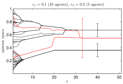
Figure 8: Two HK processes with 50 agents, where only few are open-minded (red) and the majority is closed-minded (black). The top plot is an example of extremal consensus, the bottom plot for an evolving sitting between the chairs situation.

Figures 9 and 10 show density-based dynamics for the DW model with an essentially uniform but perturbed initial distribution which correspond to the examples in Figure 7. The same effects are visual. Finally, in Figures 11 and 12 similar examples as in Figure 8 are reproduced in the density-based HK model

Figure 9: The situation of Figure 7 (top) in the density based model. Also comparable to Figure 3 with a perturbed initial distribution. $M^{\textrm{bary}}$ indicates the overall average opinion, which quantifies the overall drift.

Figure 10: The situation of Figure 7 (bottom) in the density based model. $M^{\textrm{bary}}$ indicates the overall average opinion, which quantifies the overall drift.

Figure 11: The situation of Figure 8 (top) in the density based model. $M^{\textrm{bary}}$ indicates the overall average opinion, which quantifies the overall drift. .

Figure 12: The situation of Figure 8 (bottom) in the density based model. $M^{\textrm{bary}}$ indicates the overall average opinion, which quantifies the overall drift.

5 Conclusions

It was demonstrated that societies with open- and a closed-minded agents can find consensus even when both bounds of confidence are surprisingly low. This adds a new phenomenon where diversity of agents has drastic effects.

The systematic simulations in Section 3 also shows that the example runs shown in Section 2 are generic. Effects of heterogeneity are more drastic as stated by Weisbuch et al Weisbuch.Deffuant.ea2002Meetdiscussand for the DW model where it is only claimed that the dynamics of the higher $\varepsilon$ will govern the evolution of clusters in the long run. Here we see that effects are much larger, allowing convergence to consensus when both bounds are low but different due to a subtle interplay.

The effect is to a large extent due to the symmetric initial situation around the mean opinion. The symmetry is conserved during dynamics therefore no overall drifts can occur. The examples in Section 4 show that severe drifts of the whole opinion profile may occur even if the initial distribution is random and essentially uniformly distributed. This gives rise to the speculation that severe drifting phenomena are also ubiquitous under heterogeneous bounds of confidence. So, they need not only happen in stylized situation as in Deffuant.Neau.ea2002HowCanExtremism ; Amblard.Deffuant2004roleofnetwork ; Deffuant2006ComparingExtremismPropagation . Drifting of the mean opinion also happens in opinion dynamics in the real world. The interplay of clustering and drifting (pulled by open-minded agents towards closed-minded agents) is also quite realistic in the political realm. So, these theoretical results might help to uncover hidden dynamics in real world opinion dynamics, which in turn can help to design better communication systems.

References

- [1] Ulrich Krause and Manfred Stöckler, editors. Modellierung und Simulation von Dynamiken mit Vielen Interagierenden Akteuren. Modus. Universität Bremen, 1997.
- [2] Ulrich Krause. A discrete nonlinear and non-autonomous model of consensus formation. In S. Elyadi, G. Ladas, J. Popenda, and J. Rakowski, editors, Communications in Difference Equations, pages 227–236. Gordon and Breach Pub., Amsterdam, 2000.
- [3] Rainer Hegselmann and Ulrich Krause. Opinion dynamics and bounded confidence, models, analysis and simulation. Journal of Artificial Societies and Social Simulation, 5(3):2, 2002.
- [4] Guillaume Deffuant, David Neau, Frédéric. Amblard, and Gérard Weisbuch. Mixing beliefs among interacting agents. Advances in Complex Systems, 3:87–98, 2000.
- [5] Gérard Weisbuch, Guillaume Deffuant, Frédéric Amblard, and Jean-Pierre Nadal. Meet, discuss, and segregate! Complexity, 7(3):55–63, 2002.
- [6] Patrick Groeber, Frank Schweitzer, and Kerstin Press. How groups can foster consensus: The case of local cultures. Journal of Artificial Societies and Social Simulation, 12(2):4, 2009.
- [7] Jan Lorenz. A stabilization theorem for dynamics of continuous opinions. Physica A: Statistical Mechanics and its Applications, 355(1):217–223, 2005.
- [8] Jan Lorenz and Diemo Urbig. About the Power to Enforce and Prevent Consensus by Manipulating Communication Rules. Advances in Complex Systems, 10(2):251, 2007.
- [9] Eli Ben-Naim, Paul L. Krapivsky, and Sidney Redner. Bifurcation and patterns in compromise processes. Physica D, 183:190–204, 2003.
- [10] Santo Fortunato, Vito Latora, Alessandro Pluchino, and Andrea Rapisarda. Vector opinion dynamics in a bounded confidence consensus model. International Journal of Modern Physics C, 16(10):1535–1551, 2005.
- [11] Jan Lorenz. Continuous Opinion Dynamics under bounded confidence: A Survey. Int. Journal of Modern Physics C, 18(12):1819–1838, 2007.
- [12] M. F. Laguna, Guillermo Abramson, and Dami n H. Zanette. Minorities in a model for opinion formation. Complexity, 9(4):31–36, 2004.
- [13] Vincent D. Blondel, Julien M. Hendrickx, and John N. Tsitsiklis. On the 2r conjecture for multi-agent systems. In Proceedings of the European control conference 2007 (ECC 2007), Kos (Greece), 2007.
- [14] Jan Lorenz. Continuous opinion dynamics: Insights through interactive Markov chains. In Proceedings of IASTED Conference Modelling, Simulation and Optimization MSO, 2005.
- [15] Jan Lorenz. Consensus strikes back in the Hegselmann-Krause model of continuous opinion dynamics under bounded confidence. Journal of Artificial Societies and Social Simulation, 9(1):8, 2006.
- [16] Jan Lorenz. Repeated Averaging and Bounded Confidence-Modeling, Analysis and Simulation of Continuous Opinion Dynamics. PhD thesis, Universität Bremen, March 2007.
- [17] Jan Lorenz. Fixed points in models of continuous opinion dynamics under bounded confidence. In A. Ruffing, A. Suhrer, and J. Suhrer, editors, Communications of the Laufen Colloquium on Science 2007. Shaker Publishing, 2007.
- [18] Guillaume Deffuant, David Neau, Frédéric. Amblard, and Gérard Weisbuch. How Can Extremism Prevail? A Study Based on the Relative Agreement Interaction Model. Journal of Artificial Societies and Social Simulation, 5(4):1, 2002.
- [19] Frédéric Amblard and Guillaume Deffuant. The role of network topology on extremism propagation with the relative agreement opinion dynamics. Physica A: Statistical Mechanics and its Applications, 343:725–738, 2004.
- [20] Guillaume Deffuant. Comparing Extremism Propagation Patterns in Continuous Opinion Models. Journal of Artificial Societies and Social Simulation, 9(3):8, 2006.