Phase glass and zero-temperature phase transition in a randomly frustrated two-dimensional quantum rotor model

Abstract

The ground state of the quantum rotor model in two dimensions with random phase frustration is investigated. Extensive Monte Carlo simulations are performed on the corresponding (2+1)-dimensional classical model under the entropic sampling scheme. For weak quantum fluctuation, the system is found to be in a phase glass phase characterized by a finite compressibility and a finite value for the Edwards-Anderson order parameter, signifying long-ranged phase rigidity in both spatial and imaginary time directions. Scaling properties of the model near the transition to the gapped, Mott insulator state with vanishing compressibility are analyzed. At the quantum critical point, the dynamic exponent $z_{\rm dyn}\simeq 1.17$ is greater than one. Correlation length exponents in the spatial and imaginary time directions are given by $\nu\simeq 0.73$ and $\nu_{z}\simeq 0.85$, respectively, both assume values greater than 0.6723 of the pure case. We speculate that the phase glass phase is superconducting rather than metallic in the zero current limit.

Keywords: Quantum rotor model; phase glass; Josephson junction array; quantum phase transition.

1 Introduction

Understanding the macroscopic state of a system of interacting bosons at zero temperature is of interest to the solution of a number of problems in condensed matter physics[1, 2, 3, 4]. The theory of superconductivity is built on Cooper pairs which can be treated as bosons. Mapping of flux-lines in type-II superconductors to a two-dimensional (2D) bosonic system has led to a deeper understanding of the I-V characteristics of cuprate superconductors[5, 6]. More recently, the realization of Bose-Einstein condensation (BEC) in dilute atomic alkali gases has provided an experimental means to systematically explore various types of macroscopic quantum states and transitions between them, enriching our knowledge about equilibrium and dynamic properties of strongly correlated quantum systems[7, 8, 9].

Previously, it has been established that repulsive bosons in restricted geometries (such as those confined by an optical lattice) may undergo a zero-temperature quantum phase transition from a superfluid state to a Mott insulator state as the strength of the interaction is increased[10]. The superfluid state is characterized by its well-known off-diagonal long-range order and a finite phase rigidity, whereas the Mott insulator state is characterized by zero compressibility and gapped particle excitations. Transition between the two gives over to intervening states (e.g., Bose glass or Mott glass) when disorder, either in the form of random on-site potential or random hopping coefficients are introduced[10, 11, 12, 13].

In this paper we focus on a different type of disorder, i.e., random phase frustration on the ground state properties of a 2D interacting bosonic system. Such a situation has been realized experimentally in positionally disordered Josephson junction arrays, where the frustration can be tuned by varying the strength of a transverse magnetic field[3, 14]. At sufficiently strong disorder, it has been suggested that the superfluid state changes into a new state of matter, the “phase glass” phase[15]. Although the existence of such a state is not much disputed, its precise physical properties have not been well established[15, 16].

The classical limit of the above problem can be described by a 2D XY model with random phase shifts[17]. The phase diagram of the classical model has been worked out by Nattermann et al.[18] using renormalization group methods. When the frustration is weak, only a small number of localized and tightly bound vortex-antivortex pairs are present in the classical ground state, so that long-ranged phase order is preserved at sufficiently low temperatures. However, as the frustration exceeds a certain critical value, the ground state becomes unstable against free vortex excitations due to a large distance instability[18, 19, 20, 21]. Consequently, vortices and antivortices proliferate and destroy the ordered state at all temperatures.

The gauge glass model represents an extreme case where the random frustration attains its maximum strength[22, 23]. Despite extensive studies by a number of groups[23, 24, 25, 26, 27, 28, 29, 30], the low temperature properties of the 2D model are still controversial. At the heart of the discussion is whether a certain form of glass rigidity survives despite the presence of a finite density of free vortices in the system. Numerical simulations of the gauge glass model have yielded contradictory conclusions with regard to a finite temperature glass transition. In Ref. [31], we have carried out an explicit analysis of vortex configurations in the ground and low-lying excited states of a corresponding Coulomb gas model, where the random frustration is represented by a set of randomly oriented dipoles which interact with the vortices[18, 21]. The main conclusion of the analysis is that, unlike the case of an Ising spin glass, the ground state of the 2D Coulomb gas in the random dipolar field is quite unique. The low-lying excited vortex states can be described in terms of a dilute gas of localized vortex-antivortex pairs super-imposed on a complex and critical but otherwise innocent ground state vortex configuration. Due to the disorder, the density of states of these pairs is finite at zero excitation energy. Consequently, these pairs are able to participate in dielectric screening under thermal equilibrium conditions. Renormalization group arguments show that the ground state of the gauge glass is a critical state with a phase rigidity that decays algebraically with distance. Thermal excitations of low energy vortex-antivortex pairs at temperature $T$ lead to a finite correlation length $\xi(T)$ which diverges as $T$ tends to zero. These predictions are confirmed by direct Monte Carlo simulations of the gauge glass model.

Since the power-law decay of phase rigidity with distance $r$ requires dielectric screening by excited vortex-antivortex pairs of size comparable to $r$ and the corresponding vortex movement at smaller scales, it is legitimate to ask if such a complex relaxation process can be realized in dynamic simulations and experiments. The slow dynamics for the creation and annhilation of distant vortex-antivortex pairs may indeed give rise to an apparent phase rigidity bigger than its equilibrium value. It is plausible that this type of glassy behavior is responsible for the previously reported finite temperature transition[14, 28, 29, 30], though one needs to work out the relevant energy and time scales for a detailed verification of this scenario.

Quantum fluctuations of the phase lower the core energy of vortices and antivortices and facilitate their delocalization through quantum tunneling. Sufficiently strong fluctuations of this type destroy long-ranged phase ordering as in the pure case, giving rise to the Mott insulator state. In the following we present detailed numerical results to show that, when the fluctuations are weak, the ground state of the system retains phase rigidity both in space and in time as in the classical case. This phase glass phase is characterized by a finite Edwards-Anderson order parameter, a finite compressibility, but a vanishing superfluid density or helicity modulus. We also carry out a scaling analysis of the transition to the Mott insulator state. Our results for various critical exponents are significantly different from those of the pure case, suggesting that the phase glass to the Mott insulator transition belongs to a different universality class than the three-dimensional (3D) XY model[1, 2, 10].

The paper is organized as follows. In Sec. 2, we introduce the model Hamiltonian and the mapping to the (2+1)-dimensional classical model. The procedure for performing Monte Carlo simulations under an entropic sampling scheme is outlined. Various quantities characterizing ordering in the phase glass phase are introduced. We also review briefly a general scaling theory developed by Fisher et al.[10] for the analysis of the critical behavior at the quantum phase transition of a bosonic system. Section 3 contains results from extensive Monte Carlo simulations of the (2+1)-dimensional model. The critical exponents are extracted based on a finite-size scaling analysis. Significance of these findings are discussed briefly in Sec. 4. The mapping between the 2D quantum model and the (2+1)-dimensional classical model is presented in the Appendix for easy reference.

2 The randomly frustrated quantum rotor model and its basic properties

2.1 The Hamiltonian

We consider a 2D Josephson junction array of superconducting grains in a transverse magnetic field. In a coarse-grained description, the Hamiltonian can be written as,

$$\hat{H}={E_{Q}\over 2}\sum_{i}\hat{n}_{i}^{2}-E_{J}\sum_{\langle ij\rangle}\cos(\theta_{i}-\theta_{j}-a_{ij}).$$ (1)

Here $\hat{n}_{i}$ and $\theta_{i}$ are the number operator of (excess) Cooper pairs and the phase of the superconducting order parameter on grain $i$, respectively. They satisfy the commutation relation $[\theta_{j},\hat{n}_{k}]=i\delta_{j,k}$. In the $\theta$-representation, we may write $\hat{n}_{j}=-i\partial/\partial\theta_{j}$. The first term on the right-hand-side of (1), which sums over all $N$ sites of a square lattice, represents on-site Coulomb repulsion between the Cooper pairs whose strength is specified by the charging energy $E_{Q}=4e^{2}/C$, with $C$ being the capacitance of a single grain. The second term represents Josephson coupling between neighboring islands with strength $E_{J}$, and the sum is over all nearest neighbor bonds of the lattice.

The phase shifts $a_{ij}$ in Eq. (1) are related to the vector potential ${\bf A}$ of an external magnetic field through,

$$a_{i,j}=\frac{2\pi}{\Phi_{0}}\int_{i\rightarrow j}{\bf A}\cdot d{\bf l}.$$ (2)

Here ${\Phi_{0}}=hc/(2e)$ is the elementary flux quantum. In the present paper we shall focus on the maximally frustrated case where the random phase shifts $a_{ij}$’s are uniformly distributed on the interval $[0,2\pi)$ and uncorrelated from bond to bond. The case $a_{ij}=0$ corresponds to the well-known quantum rotor model[2].

The Hamiltonian (1) is invariant under a global rotation, $\theta_{i}\rightarrow\theta_{i}+c$, all $i$. This symmetry is important in the discussion of the low energy excitations of the system.

2.2 Mapping to a (2+1)-dimensional classical model

It is well-known that, as far as the thermal equilibrium properties are concerned, the quantum rotor model can be mapped to a (2+1)-dimensional classical system using the Trotter formula[1, 11]. This mapping forms the basis of our quantum Monte Carlo calculation.

Let us start with the partition function

$$Z(\beta)={\rm Tr\ }\exp(-\beta\hat{H}),$$ (3)

where $\beta=1/(k_{B}T)$ is the inverse temperature. Following the procedure described in Appendix A, we arrive at a classical model defined by the action (33). The model can be brought into a dimensionless form through the introduction of $z=\tau/\tau_{0}$ as the coordinate in the third direction, where $\tau_{0}=\hbar/\sqrt{E_{Q}E_{J}}$. After the transformation, we obtain

$$Z(\beta)=\int[{\cal D}\theta]\exp\Bigl{[}-{1\over K}\int_{0}^{L_{z}}dzH_{P}\Bigr{]},$$ (4)

where $L_{z}=\beta\hbar/\tau_{0}=\sqrt{E_{J}E_{Q}}/k_{B}T$, $K=\sqrt{E_{Q}/E_{J}}$, and

$$H_{P}={1\over 2}\sum_{j}\Bigl{(}{d\theta_{j}\over dz}\Bigr{)}^{2}-\sum_{\langle ij\rangle}\cos(\theta_{i}-\theta_{j}-a_{ij}).$$ (5)

In our Monte Carlo simulations of the quantum rotor model, we choose a discretization along the $z$-axis with $dz=1$ and approximate $d\theta_{j}/dz$ by $\theta_{j}(z+1)-\theta_{j}(z)$. This procedure appears to be rather adequate for the exploration of the phase glass phase and the transition to the Mott insulator state. With this choice of $dz$, the critical point $K_{c}$ of the discrete model is expected to be somewhat different from that of the original model, though we believe the large-distance properties are not affected. The boundary conditions in the $xy$-plane are chosen to be periodic, while Eq. (34) is used along the $z$-direction. With these specifications, we obtain a classical (2+1)-dimensional lattice model where $K$ plays the role of a “quantum temperature”. As such, the model can be simulated using the entropic sampling scheme[32]. Since the algorithm allows the system to explore configurations over a broad range of values of the classical action (5) in a single simulation, it has a better chance to generate statistically independent samples for the calculation of thermal averages, which may become a problem for conventional Monte Carlo methods in the glass phase. In addition, once equilibrated, values of any measurable quantity over a broad range of $K$ values can be readily calculated. This is particularly useful for analyzing the zero-temperature quantum phase transition. More details about our implementation of the scheme can be found in Ref. [33].

2.3 Helicity modulus and compressibility

Helicity modulus can be related to the superfluid density and hence provides a direct measure of the superconducting order. It is defined by considering the change of the free energy under a phase twist across the system. Quite generally, such a twist modifies the action to $\tilde{H}_{P}=H_{P}+\delta H_{P}$. The change in the free energy, to the second order in $\delta H_{P}$, is given by,

$$\delta F = -k_{B}T\ln(\tilde{Z}/Z)$$ (6)

$$= -k_{B}T\ln\Bigl{\langle}\exp(-{1\over K}\int_{0}^{L_{z}}dz\delta H_{P})\Bigr{\rangle}$$

$$\simeq E_{J}\langle\delta H_{P}\rangle-{E_{J}^{2}\over 2k_{B}T}\Bigl{[}\Bigl{\langle}\Bigl{(}{1\over L_{z}}\int_{0}^{L_{z}}dz\delta H_{P}\Bigr{)}^{2}\Bigr{\rangle}-\langle\delta H_{P}\rangle^{2}\Bigr{]}.$$

Here $\langle\cdot\rangle$ denotes thermal average. For a twist $\Delta_{x}$ per bond in the $x$-direction, we have

$$\delta H_{P} = \Delta_{x}\sum_{i}\sin(\theta_{i+x}-\theta_{i}+a_{i,x})+{1\over 2}\Delta_{x}^{2}\sum_{i}\cos(\theta_{i}-\theta_{i+x}-a_{i,x})+\ldots$$ (7)

Writing $\delta F={1\over 2}N\rho_{s}E_{J}\Delta_{x}^{2}$, we obtain the following expression for the helicity modulus,

$$\rho_{s} = \langle\overline{\cos(\theta_{x}-\theta_{i+x}-a_{i,x})}\rangle-{N\over K}\int_{0}^{L_{z}}dz\bigl{[}\langle\bar{J}_{x}(0)\bar{J}_{x}(z)\rangle-\langle\bar{J}_{x}(0)\rangle^{2}\bigr{]}.$$ (8)

Here $\bar{J}_{x}(z)=N^{-1}\sum_{i}\sin(\theta_{i+x}(z)-\theta_{i}(z)+a_{i,x})$ is the average current along the $x$-direction in layer $z$, and the overline bar denotes spatial average.

The compressibility $\kappa$ is related to the change in free energy for a phase twist $\Delta$ in the $z$-direction[10]. The corresponding change in $H_{P}$ is given by,

$$\delta H_{p}=\Delta\sum_{i}{d\theta_{i}\over dz}+{1\over 2}N\Delta^{2}.$$ (9)

Inserting Eq. (9) into Eq. (6), and noting that $\int_{0}^{L_{z}}dz(d\theta_{i}/dz)=\theta_{i}(L_{z})-\theta_{i}(0)=2\pi n_{i}$, where $n_{i}$ is the number of turns the angle on site $i$ makes along the $z$-direction, we obtain

$$\delta F\simeq{1\over 2}NE_{J}\Delta^{2}-{E_{J}^{2}\over 2k_{B}T}\Bigl{\langle}\Bigl{(}{1\over L_{z}}\sum_{i}2\pi n_{i}\Bigr{)}^{2}\Bigr{\rangle}={1\over 2}NE_{J}\kappa\Delta^{2},$$ (10)

where

$$\kappa=1-{4\pi^{2}\over KNL_{z}}\Bigl{\langle}\Bigl{(}\sum_{i}n_{i}\Bigr{)}^{2}\Bigr{\rangle}.$$ (11)

Here $\langle n_{i}\rangle=0$ due to symmetry.

2.4 The Edwards-Anderson order parameter

The Edwards-Anderson order parameter for the quantum rotor model can be defined via

$$q_{\rm EA}=\lim_{t\rightarrow\infty}\overline{\langle e^{i[\theta_{j}(t)-\theta_{j}(0)]}\rangle},$$ (12)

where $e^{i\theta_{j}(t)}=e^{-i\hat{H}t/\hbar}e^{i\theta_{j}}e^{i\hat{H}t/\hbar}$.

Consider now the auto-correlation function in imaginery time,

$$C(\tau,\beta) = \overline{\langle e^{\hat{H}\tau/\hbar}e^{i\theta_{j}}e^{-\hat{H}\tau/\hbar}e^{-i\theta_{j}}\rangle}$$ (13)

$$= {1\over Z}{\rm Tr}\bigl{[}\overline{e^{-(\beta\hbar-\tau)\hat{H}/\hbar}e^{i\theta_{j}}e^{-\hat{H}\tau/\hbar}e^{-i\theta_{j}}}\bigr{]}$$

$$= \overline{\langle e^{i[\theta_{j}(z)-\theta_{j}(0)]}\rangle},$$

where $z=\tau/\tau_{0}$, and the last average is carried out in the (2+1)-dimensional classical ensemble. At $T=0$, the long-time limit $t\rightarrow\infty$ can be replaced by the limit $\tau\rightarrow\infty$. Hence we may write,

$$q_{\rm EA}=\lim_{L_{z}\rightarrow\infty}C(L_{z}/2,L_{z}).$$ (14)

2.5 Scaling properties near the Mott insulator transition

The Mott insulator state corresponds to the “high temperature” phase of the (2+1)-dimensional classical model where quantum phase fluctuations lead to a vanishing superfluid density, vanishing compressibility, and an exponentially decaying phase-correlation function in imaginary time. Due to the anisotropic form of (5), two different lengths $\xi$ and $\xi_{z}$ are needed to describe the spatial and temporal correlations in the system. As $K$ approaches its critical value $K_{c}$ at the transition from the Mott insulator to the phase glass, both quantities are expected to diverge as

$$\xi\sim|K-K_{c}|^{-\nu},\qquad\xi_{z}\sim|K-K_{c}|^{-\nu_{z}},$$ (15)

where $\nu$ and $\nu_{z}$ are the respective exponents. Since $\xi_{z}^{-1}$ corresponds to a characteristic energy or frequency scale in the quantum rotor model, the ratio $z_{\rm dyn}=\nu_{z}/\nu$ defines the dynamical exponent at the transition. In the phase glass phase, both $\xi$ and $\xi_{z}$ are expected to be infinite. The exponent $z_{\rm dyn}^{\rm PG}$ of the phase glass phase, which may be different from its value at the transition, can be determined from suitable finite-size scaling properties.

Earlier, Fisher et al.[10] proposed a general scaling theory for the quantum phase transition in bosonic systems. In particular, based on the assumption that the singular part of the free energy (or ground state energy in the quantum model) in a correlated volume $\xi^{d}\xi_{z}$ is of order $K_{c}$, they determined the scaling dimensions of the superfluid density and compressibility in the transition region,

$$\rho_{s}\sim|K-K_{c}|^{\zeta},\qquad\kappa\sim|K-K_{c}|^{\zeta_{z}},$$ (16)

where $d$ is the spatial dimension, and

$$\zeta=(d-2)\nu+\nu_{z},\qquad\zeta_{z}=d\nu-\nu_{z}$$ (17)

are the scaling exponents.

The auto-correlation function (13), on the other hand, is expected to decay as a power law at $K=K_{c}$,

$$C(\tau,\infty)\sim\tau^{-1-(d-2+\eta)/z_{\rm dyn}},$$ (18)

where $\eta$ is a new exponent. Scaling arguments then yield,

$$q_{\rm EA}\sim|K-K_{c}|^{(d-2+\eta)\nu+\nu_{z}}.$$ (19)

For the (2+1)-dimensional classical model, the “specific heat” $c_{V}(K)=-K\partial^{2}f/\partial K^{2}$ with $f=F/(NL_{z})$ is expected to exhibit singular behavior at $K_{c}$. From the above assumption for the singular part of the free energy $f_{s}\sim\xi^{-d}\xi_{z}^{-1}$, one obtains the specific heat exponent,

$$\alpha=2-d\nu-\nu_{z}.$$ (20)

In the pure case $a_{ij}=0$ and $d=2$, the quantum rotor model is mapped to the 3D classical XY model. Consequently $z_{\rm dyn}=1$, and $\zeta=\zeta_{z}=\nu=\nu_{z}$, i.e., $\rho_{s}$ and $\kappa$ scale the same way as $\xi_{z}^{-1}$ which provides the only energy scale of the problem. Numerical calculations have yielded $\nu_{\rm 3DXY}\simeq 0.6723$[34]. From the scaling relation $\gamma=(2-\eta)\nu\simeq 1.319$ we obtain $\eta_{\rm 3DXY}\simeq 0.04$. The exponent $\alpha_{\rm 3DXY}\simeq-0.017$ is also very small. One of our numerical tasks below is to check whether the same set of exponent values apply to the phase glass to the Mott insulator transition.

3 Simulation results

We have carried out extensive Monte Carlo simulations of the (2+1)-dimensional classical model (5) under the entropic sampling scheme. The system is chosen to be a cubic lattice of $L_{z}$ layers each containing $N=L^{2}$ sites in the $xy$-plane. Test runs were performed on the unfrustrated quantum rotor model (referrd to below as the pure model) which generated results in good agreement with previous studies on the superfluid to the Mott insulator transition at $K_{c0}\simeq 2.55$. Unless explicitly stated, the data presented below for the disordered case are obtained from averages over 30 to 100 samples at any given size. This seems to be sufficient for illustrating the behavior of the phase glass phase and for determining the critical exponents of the transition within the limit set by the system size we are able to investigate.

Figure 1(a) shows the “specific heat” data for the pure model against $K$ for six different system sizes. The cusp singularity at $K_{c0}$ with a very small exponent $\alpha$ is evident. In comparison, as seen in Fig. 1(b), the singularity is much weaker in the randomly frustrated model. The dashed line in the figure with

$$\alpha\simeq-0.3$$ (21)

indicates a possible behavior in the infinite size limit that is consistent with our data, though in general the critical amplitudes on the two sides of the transition need not be the same.

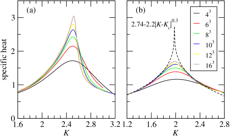
Figure 1: The “heat capacity” against $K=\sqrt{E_{Q}/E_{J}}$ for (a) The pure model and (b) the randomly frustrated model at six different system sizes as indicated in the figure. The dashed line in (b) represents a possible behavior at infinite system size. Here $K_{c}=1.98$.

Figure 2 shows the helicity modulus $\rho_{s}$ and the compressibility $\kappa$ of a $16^{3}$ system against $K$ for four different disorder realizations. Both quantities become vanishingly small when $K>K_{c}\simeq 1.98$. At smaller values of $K$, $\rho_{s}$ is strongly sample-dependent and takes on both positive and negative values. For a given sample, $\rho_{s}$ may also be a non-monotonic function of $K$. The disorder-averaged value of $\rho_{s}$, on the other hand, remains close to zero. A nonzero $\rho_{s}$ for individual samples signifies “freezing” of vortex loops that enables long-ranged phase rigidity to develop. To understand the origin of negative values for $\rho_{s}$, one may consider a more general twist boundary condition in each layer, $\theta_{x+L,y}=\theta_{x,y}+\Delta_{x}$ and $\theta_{x,y+L}=\theta_{x,y}+\Delta_{y}$ (see, e.g., Ref.[25]). Due to the random phase shifts, the minimum of the free energy is in general achieved at some nonzero values of $\Delta_{x}$ and $\Delta_{y}$. Depending on the particular choice of the random phase shifts, the curvature $\rho_{s}$ of the free energy at $\Delta_{x}=\Delta_{y}=0$ may take on positive or negative values. A sign change can occur when one or more vortices are relocated on the scale of the system size. Such a move does not alter the local phase gradients in a significant way and hence costs only a small amount of energy. As $K$ is varied, one may envisage a change in the relative statistical significance of configurations that differ in this way, leading to the observed non-monotonic behavior.

In contrast, the compressibilities of the four samples differ only slightly from one another, with no significant broadening near $K_{c}$. Other quantities, such as the specific heat and correlation functions, show the same behavior. Therefore the system is expected to be self-averaging in the large-size limit.

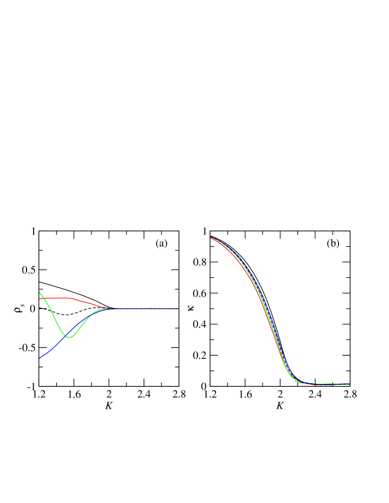
Figure 2: (a) The helicity modulus and (b) the compressibility against $K=\sqrt{E_{Q}/E_{J}}$ for four disorder realizations at $L=L_{z}=16$. The dashed line in each case indicates average over the four samples.

The critical exponents for the transition can be determined by applying suitable finite-size scaling forms. Below we shall perform the analysis using $L_{z}$ as the scaling variable. The general finite-size scaling ansatz of a quantity $X$ then reads,

$$X(K,L,L_{z})=L_{z}^{-x/\nu_{z}}\hat{X}\bigl{(}(K-K_{c})L_{z}^{1/\nu_{z}},L^{z_{\rm dyn}}/L_{z}\bigr{)},$$ (22)

where $x$ is the critical exponent for the quantity $X$. Equation (22) is quite difficult to use in general due to the simultaneous presence of two scaled variables. However, as we shall see below, the exponent $z_{\rm dyn}$ is quite close to (but larger than) one so that, for the range of system sizes considered, the second argument is approximately constant and does not affect significantly the value of the function. The validity of this assumption is justified a posteriori by the consistency of the exponent values obtained.

Figure 3(a) shows the disorder averaged compressibility $\kappa$ against $K$ for six different system sizes, ranging from $L=L_{z}=4$ to $L=L_{z}=16$. At $K=K_{c}$ (as indicated by the dashed line in the figure), the decay of $\kappa$ against $L_{z}$ can be fitted to a power law with an exponent $\zeta_{z}/\nu_{z}=0.7\pm 0.1$. From the scaling relation (17) we obtain

$$z_{\rm dyn}=1.17\pm 0.07.$$ (23)

Combining this result with our previous estimate $\alpha=2-2\nu-\nu_{z}\simeq-0.3$ yields

$$\nu\simeq 0.73,\qquad\nu_{z}\simeq 0.85,\qquad\zeta_{z}=2\nu-\nu_{z}\simeq 0.61.$$ (24)

The scaling plot shown in Fig. 3(b) is generated using these exponent values. A reasonable data collapse is seen. Note that there is a slight increase in the slope of the curves with increasing $L$ or $L_{z}$, which is consistent with the expected trend associated with a gradual increase of the scaled variable $L^{z_{\rm dyn}}/L_{z}$ for this set of data.

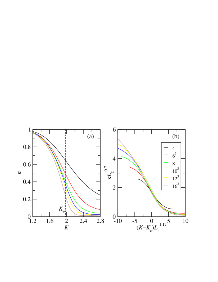
Figure 3: (a) The disorder averaged compressibility for six different system sizes $L=L_{z}=4,6,8,10,12,$ and 16. (b) A scaling plot using the exponents discussed in the text.

We now examine the behavior of the Edwards-Anderson order parameter $q_{\rm EA}=C(L_{z}/2,L_{z})$. As shown in Fig. 4(a), the effect of finite size is more pronounced here as compared to $\kappa$ in Fig. 3(a). Also, the dependence of $q_{\rm EA}$ on $L_{z}$ at a finite $L$ is complicated by the fact that, in a finite system, the spectrum of $\hat{H}$ is always discrete so that, strictly speaking, $q_{\rm EA}$ as defined by (14) vanishes in the limit $\beta\rightarrow\infty$. Nevertheless, for the choice $L_{z}=L$, we observe that data at a given $K<K_{c}$ can be well fitted by a quadratic function in $1/L_{z}$, as shown in Fig. 4(b). Using such an extrapolation procedure, we obtain a value for $q_{\rm EA}$ at each $K$ in the infinite size limit as indicated by the dashed line in Fig. 4(a). The approach of $q_{\rm EA}$ to zero as $K$ tends to $K_{c}$ can be described by a power-law with an exponent 0.8. Comparing with Eq. (19) and the values mentioned above for $\nu$ and $\nu_{z}$, this result is consistent with a small value for the exponent $\eta$.

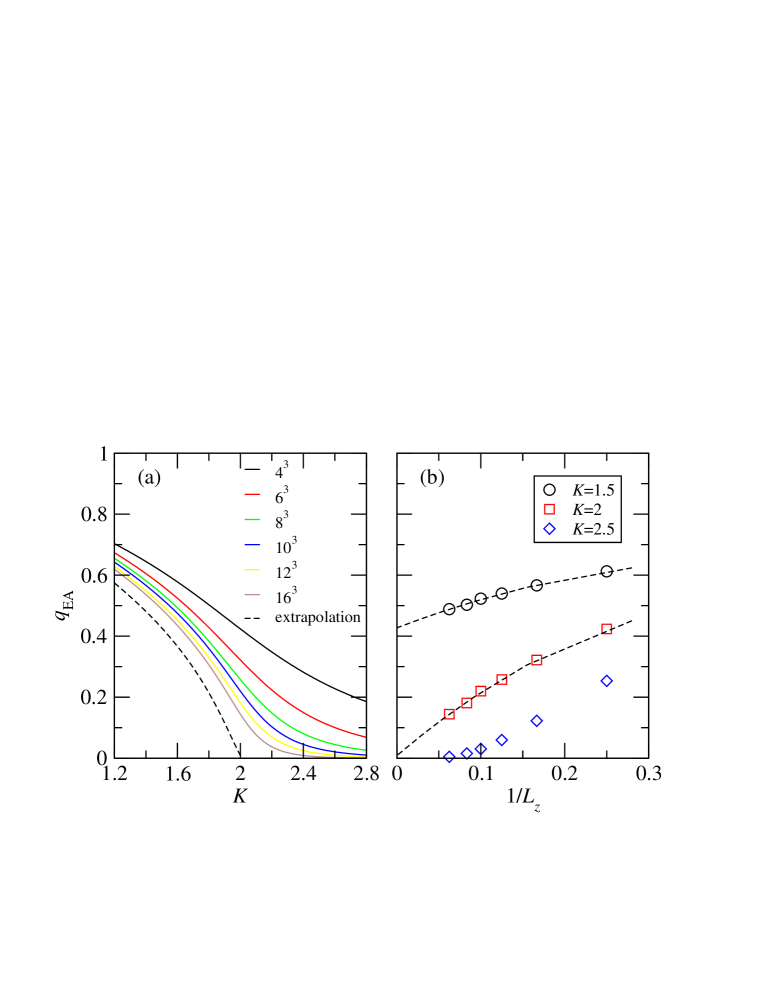
Figure 4: (a) The disorder averaged Edwards-Anderson order parameter for six different system sizes $L=L_{z}=4,6,8,10,12,$ and 16. Dashed line indicates extrapolated value using a quadratic fit. (b) The dependence of $q_{\rm EA}$ on $L_{z}$ for selected values of $K$.

4 Summary and discussions

The main findings of our numerical investigation of the quantum rotor model at maximal random frustration are summarized as follows. When the charging energy $E_{Q}$ (or boson repulsion) is small compared to the Josephson energy $E_{J}$ (or boson hopping energy), the system behaves quite similarly to the classical gauge glass model at zero temperature. The compressibility $\kappa$ is positive and increases with decreasing $K=\sqrt{E_{Q}/E_{J}}$. The Edwards-Anderson order parameter $q_{\rm EA}$ also assumes a finite value, signifying long-ranged phase ordering in time. The $1/\tau$ (or $1/L_{z}$) correction to $q_{\rm EA}$ in imaginary time [see Fig. 4(b)] is the same as in the isotropic 3D XY model, suggesting a dynamic exponent $z_{\rm dyn}^{PG}=1$ and linear dispersion for the gapless phase modes. These properties do not seem to be affected by the power-law decaying spin-glass stiffness in the spatial direction obtained previously[25, 26, 31]. Our results suggest that quantum tunneling between the classically distinct low energy vortex states as discussed in Ref.[31] is suppressed at large distances in the phase glass. The existence of spatial (glassy) phase order is also supported by a nonvanishing helicity modulus $\rho_{s}$ below $K_{c}$ in individual samples, though due to the random phase shifts, $\rho_{s}$ does not have a definitive sign. These observations suggest that diffusive transport of vortices under an applied current is unlikely in the present model except perhaps at $K=K_{c}$, casting doubt on the link between the phase glass and bose metal when the only quenched disorder in the system is in the form of random phase frustrations[15].

We have also attempted to determine the critical exponents characterizing the phase glass to the Mott insulator transition. Due to the relatively small system sizes available, the estimated values of the exponents should be considered as only tentative. With this caveat in mind, our data are broadly consistent with a dynamic exponent $z_{\rm dyn}\simeq 1.17\pm 0.07$ greater than one, and correlation length exponents $\nu\simeq 0.73$ and $\nu_{z}\simeq 0.85$, both greater than their value 0.6723 in the pure case. It would be interesting to confirm (or disprove) these results with more efficient numerical algorithms applied to the model.

Appendix A Path integral representation of the partition function

Following the standard procedure, we define $\hat{M}=\exp(-\beta\hat{H}/n)$ and write

$$Z(\beta)={\rm Tr}(M^{n}).$$ (25)

When the integer $n$ is large, we may write

$$\hat{M}=\exp(-\beta(\hat{H}_{Q}+\hat{H}_{J})/n)\simeq\exp(-\beta\hat{H}_{Q}/n)\exp(-\beta\hat{H}_{J})/n),$$ (26)

where

$$\hat{H}_{Q} = {E_{Q}\over 2}\sum_{i}\hat{n}_{i}^{2}=-{E_{Q}\over 2}\sum_{i}{\partial^{2}\over\partial\theta_{i}^{2}},$$ (27)

$$\hat{H}_{J} = -E_{J}\sum_{\langle ij\rangle}\cos(\theta_{i}-\theta_{j}-a_{ij}),$$ (28)

are the Coulomb and Josephson energies, respectively, which do not commute.

Let $|\{\theta\}\rangle$ be a state where each rotor $j$ has a definitive phase $\theta_{j}\in[0,2\pi)$, and $|\{m\}\rangle$ be a state where each rotor $j$ has a definitive angular momentum $m_{j}=0,\pm 1,\pm 2,\ldots$ The matrix elements of $\hat{M}$ can be written as,

$$M(\{\theta^{\prime}\},\{\theta\}) \equiv \langle\{\theta^{\prime}\}|\hat{M}|\{\theta\}\rangle$$ (29)

$$\simeq \langle\{\theta^{\prime}\}|\exp(-\beta\hat{H}_{Q}/n)\exp(-\beta\hat{H}_{J})/n)|\{\theta\}\rangle$$

$$= \langle\{\theta^{\prime}\}|\exp(-\beta\hat{H}_{Q}/n)\sum_{\{m\}}|\{m\}\rangle\langle\{m\}|\exp(-\beta\hat{H}_{J})/n)|\{\theta\}\rangle$$

$$= \exp\Bigl{[}{\beta E_{J}\over n}\sum_{\langle ij\rangle}\cos(\theta_{i}-\theta_{j}-a_{ij})\Bigr{]}$$

$$\times\sum_{\{m\}}\exp\Bigl{[}-{\beta E_{Q}\over 2n}\sum_{j}m_{j}^{2}+i\sum_{j}m_{j}\delta\theta_{j}\Bigr{]},$$

where $\delta\theta_{j}=\theta_{j}^{\prime}-\theta_{j}$ and we have used $\langle\{\theta\}|\{m\}\rangle=\exp(i\sum_{j}m_{j}\theta_{j})$. With the help of the Poisson summation formula,

$$\sum_{m=0,\pm 1,\pm 2,\ldots}f(m)=\sum_{s=0,\pm 1,\pm 2,\ldots}\int duf(u)\exp(2\pi ius),$$ (30)

the sum over the angular momentum eigenstates $\{m\}$ can be carried out,

$$\sum_{\{m\}}\exp\Bigl{[}-{\beta E_{Q}\over 2n}\sum_{j}m_{j}^{2}+i\sum_{j}m_{j}\delta\theta_{j}\Bigr{]}$$

$$= \sum_{\{s\}}\int[du]\exp\Bigl{[}-{\beta E_{Q}\over 2n}\sum_{j}u_{j}^{2}+i\sum_{j}u_{j}(\delta\theta_{j}+2\pi s_{j})\Bigr{]}$$

$$= A\sum_{\{s\}}\exp\Bigl{[}-{n\over 2\beta E_{Q}}\sum_{j}(\delta\theta_{j}+2\pi s_{j})^{2}\Bigr{]},$$ (31)

where $A$ is a numerical constant.

With these preparations we may carry out the matrix multiplication and trace in Eq. (25) to obtain,

$$Z(\beta) = \lim_{n\rightarrow\infty}\int[{\cal D}\theta]\prod_{k=0}^{n-1}M\bigl{(}\{\theta(\tau_{k+1})\},\{\theta(\tau_{k})\}\bigr{)},$$ (32)

$$= \int[{\cal D}\theta]\exp\Bigl{[}-{1\over\hbar}\int_{0}^{\beta\hbar}d\tau H_{c}\Bigr{]},$$

where $\tau_{k}=k\hbar\beta/n$ is the imaginery time coordinate and

$$H_{c}={\hbar^{2}\over 2E_{Q}}\sum_{j}\dot{\theta}_{j}^{2}-E_{J}\sum_{\langle ij\rangle}\cos(\theta_{i}-\theta_{j}-a_{ij})$$ (33)

is the classical action. The integration over the $\theta_{j}(\tau_{k})$’s are on the infinite domain $(-\infty,\infty)$ for all $k$ except at $k=0$, where the domain $[0,2\pi)$ is taken instead. This procedure takes care of the sum over the $s_{j}$’s as in Eq. (31). Note that

$$\theta_{j}(\beta\hbar)=\theta_{j}(0)\quad{\rm mod}\ 2\pi.$$ (34)

References

References

- [1] S. L. Sondhi, S. M. Girvin, J. P. Carini, and D. Shahar, Rev. Mod. Phys. 69, 315 (1997).
- [2] S. Sachdev, Quantum Phase Transitions, Cambridge University Press (1999).
- [3] R.S. Newrock, C. J. Lobb, U. Geigenmüller, and M. Octavio, Solid State Phys. 54, 263 (2000).
- [4] A. J. Leggett, Rev. Mod. Phys. 73, 307 (2001).
- [5] D. R. Nelson, Phys. Rev. Lett. 60, 1973 (1988); D. R. Nelson and V. M. Vinokur, Phys. Rev. B 48, 13060 (1993).
- [6] G. Blatter, M. V. Feigel’man, V. B. Geshkenbein, A. I. Larkin, and V. M. Vinokur, Rev. Mod. Phys. 66, 1125 (1994).
- [7] N. R. Cooper, N. K. Wilkin and J. M. F. Gunn, Phys. Rev. Lett. 87, 120405 (2001).
- [8] T.-L. Ho and E. J. Mueller, Phys. Rev. Lett. 89, 050401 (2002).
- [9] O. Morsch and M. Oberthaler, Rev. Mod. Phys. 78, 179 (2006).
- [10] M. P. A. Fisher, P. B. Weichman, G. Grinstein, and D. S. Fisher, Phys. Rev. B 40, 546 (1989).
- [11] M. Wallin, E. S. Sørensen, S. M. Girvin, and A. P. Young, Phys. Rev. B 49, 12115 (1994).
- [12] N. Prokof’ev and B. Svistunov, Phys. Rev. Lett. 92, 015703 (2004).
- [13] P. Sengupta and S. Haas, Phys. Rev. Lett. 99, 050403 (2007).
- [14] Y.-J. Yun, I.-C. Baek, and M.-Y. Choi, Europhys. Lett. 76, 271 (2006).
- [15] D. Dalidovich and P. Phillips, Phys. Rev. Lett. 89, 027001 (2002); P. Phillips and D. Dalidovich, Phys. Rev. B 68, 104427 (2003); Science 302, 243 (2003).
- [16] R. Ikeda, J. Phys. Soc. Jap. 76, 064709 (2007).
- [17] M. Rubinstein, B. Shraiman, and D. R. Nelson, Phys. Rev. B 27, 1800 (1983).
- [18] T. Nattermann, S. Scheidl, S. E. Korshunov, and M. S. Li, J. Phys. (France) I 5, 565 (1995).
- [19] S. E. Korshunov, Phys. Rev. B 48, 1124 (1993).
- [20] M. -C. Cha and H. A. Fertig, Phys. Rev. Lett. 74, 4867 (1995).
- [21] L.-H. Tang, Phys. Rev. B 54, 3350 (1996).
- [22] C. Ebner and D. Stroud, Phys. Rev. B 31, 165 (1985).
- [23] M. P. A. Fisher, T. A. Tokuyasu and A. P. Young, Phys. Rev. Lett. 66, 2931 (1991).
- [24] J. D. Reger and A. P. Young, J. Phys. A 26, 1067 (1993).
- [25] N. Akino and J. M. Kosterlitz, Phys. Rev. B 66, 054536 (2002).
- [26] H. G. Katzgraber, Phys. Rev. B 67, 180402(R) (2003).
- [27] M. Nikolaou and M. Wallin, Phys. Rev. B 69, 184512 (2004).
- [28] M. Y. Choi and S. Y. Park, Phys. Rev. B 60, 4070 (1999).
- [29] B. J. Kim, Phys. Rev. B 62, 644 (2000).
- [30] P. Holme, B. J. Kim, and P. Minnhagen, Phys. Rev. B 67, 104510 (2003).
- [31] L.-H. Tang and P. Tong, Phys. Rev. Lett. 94, 207204 (2005).
- [32] B. A. Berg and T. Neuhaus, Phys. Rev. Lett. 68, 9 (1992).
- [33] L.-H. Tang, in Computational Physics: Proceedings of the Joint Conference of ICCP6 and CCP2003, ed. by X.-G. Zhao, S. Jiang, and X.-J. Yu, Rinton Press (2006).
- [34] A. Cucchieri, J. Engels, S. Holtmann, T. Mendes, and T. Schultz, J. Phys. A 35, 6517 (2002).