Low excitation structure of ¹⁰B probed by scattering of electron and of 197 MeV polarized protons

Abstract

Cross-section and analyzing power data from 197 MeV $(p,p^{\prime})$ scattering and longitudinal and transverse form factors for electron scattering to low lying states in ¹⁰B have been analyzed as tests of the structure of the nuclear states when they are described using a no-core $(0+2)\hbar\omega$ shell model. While the results obtained from the shell model clearly show the need of other elements, three-body forces in particular, to explain the observed spectrum, the reasonable level of agreement obtained in the analyses of the scattering data suggest that the wave functions from our shell model with only a two-body potential are credible. Any changes to the wave functions with the introduction of three-body forces in the shell model Hamiltonian therefore should be relatively minor.

I Introduction

In a recent paper Betker et al. (2005), cross sections and spin observables were measured for the elastic and inelastic scattering of polarized protons from ¹⁰B at an energy of 197 MeV. In addition data from the charge exchange $(p,n)$ reaction to the ground state of ¹⁰C were taken at 186 MeV Wang et al. (1993); which ground state can be considered as the isobaric analogue of the $1^{+};T=1$ 1.74 MeV state in ¹⁰B. Complementing these proton scattering data are those from measurements Cichocki et al. (1995) of the longitudinal and transverse form factors of electron scattering from ¹⁰B. Such a complementary set of data provides an opportunity to assess the quality of model structures of ¹⁰B, if one has appropriate means to analyze that data. For incident protons of energies $\sim 200$ MeV, elastic and inelastic scattering observables has been predicted well with a $g$-folding model for the optical potential and the distorted wave approximation (DWA) built with the same effective two-nucleon ($NN$) interaction Amos et al. (2000). The electron scattering form factors from such a light mass nucleus also have been predicted well when allowance is made of a number of corrections and effective operators Karataglidis et al. (1995) within the Born approximation. Crucial in finding good predictions with these reaction models has been the use of very good wave functions for the states of the target nuclei. With light mass nuclei there are many models that give such and herein we use one: a no-core complete $(0+2)\hbar\omega$ shell model using the fitted interactions of Millener and Kurath Warburton and Millener (1989).

What makes ¹⁰B a difficult, and at the same time very interesting, nuclear target in analyses of proton scattering data, is that it has a ground state spin of $3^{+}$. In all reactions then, save for the excitation of $0^{+}$ states but including elastic scattering, multiple angular momentum transfer values are possible. With elastic scattering in particular, all transfer values from 0 to 6 are possible.

There are a number of studies Amos et al. (2000); Hannen et al. (2003) that show the need to use large space models of structure to adequately analyze scattering data. For light mass nuclei in particular, now that no-core, and complete basis, shell model evaluations are viable, it is of little use to restrict evaluations of structure and/or scattering to a $0\hbar\omega$ scheme despite the convenience of doing so in calculations. Such has been known for decades of course, being shown in the guise of the large effective charges required with such simple models to match electromagnetic transition data. Worse is that larger space calculations bring into the nuclear state descriptions, single particle wave functions that have more nodes. Such can influence properties which are (linear) momentum dependent, such as electron scattering form factors. Scaling electron scattering form factors to find the $B(E2,q)$ Amos et al. (2000) demonstrates that most clearly. Concerning the data of interest, Betker et al. Betker et al. (2005) and Cichocki et al. Cichocki et al. (1995) acknowledge the problems of using the limited-space, shell model wave functions that they chose in their analyses. The quite diverse scalings they require to match data reflect that. Their results indicate the implicit momentum transfer dependence of effective charges also.

Besides the limited structure used, there are other features of the previous analyses of the proton scattering data Betker et al. (2005) that are of concern. Of those, a major one is that the distorted wave impulse approximation (DWIA) was used. For incident energies to 200 MeV that approximation is not really appropriate Amos et al. (2000). First there is the associated loss of, or gross approximation to, exchange scattering amplitudes. Also phenomenological, local optical model potentials were used to determine the distorted wave functions of relative motion and those are known to be too large through the nuclear volume due to inadequate representation of nonlocal effects. Often the argument is used that a quality fit to the elastic scattering data justifies the use of the relative motion wave functions generated from phenomenological, local, optical potentials. But such fits only require specification of a suitable set of phase shifts and they are determined from the asymptotic properties of the distorted waves. The credibility of the distorted wave functions through the volume of the nucleus, properties needed in evaluation of inelastic scattering amplitudes, cannot be assured thereby. Finally, the impulse approximation does not give, or approximate well, the important effects due to specific knock-out (exchange) amplitudes. Even at 200 MeV, such have momentum transfer properties quite different to those of the direct scattering matrix elements, and, worse, often the direct and exchange amplitudes destructively interfere Amos et al. (2000). Given the large set of uncertainties in those analyses, one can have little confidence about conclusions drawn, whether about the structure of the target or of a need for additional processes such as channel coupling. Thus we have reanalyzed the data Betker et al. (2005) using a $g$-folding model of the optical potential (for $I=0$ contributions to elastic scattering) and the DWA for inelastic scattering. The non-zero angular momentum contributions to elastic scattering have been evaluated also in the DWA. We have used the $g$-folding model Amos et al. (2000) for the (nonlocal) optical potentials with the Melbourne effective $NN$ force defining the $g$-matrices. Raynal’s DWBA98 code Raynal (1998), which allows use of that medium, complex, and energy dependent mix of central, $NN$ spin-orbit, and $NN$ tensor forces has been used to give most results of proton induced scattering.

We have not sought to make a coupled-channel study. At much lower energies, where discrete state effects are known to influence scattering, a coupled-channel model of scattering is essential. An appropriate one, which ensures that the Pauli principle is satisfied even with a collective model prescription for the coupling, now exists and has been used to explain compound nucleus structure even in exotic, radioactive light mass systems Amos et al. (2003); Canton et al. (2006). However, for medium energies, such as at 197 MeV we consider herein, coupling between the low excitation energies in the target is not expected to be important, nor has there been any need for such when a good model of structure, and a reasonable $NN$ force, were used in evaluations. That is so at least for cross sections usually greater than about 0.1 mb/sr. There has been a number of papers dealing with scattering using coupling to the continuum, the so-called CDCC method. The results have been quite good but there are a number of problems with the approach as it is to date. First, and perhaps most crucially, the evaluations do not treat the effects of the Pauli principle adequately. While there have been attempts using equivalent localizations of those effects, the true non-locality caused by the indistinguishableness of the emergent nucleon with those left in the target gives scattering amplitudes that have different momentum transfer properties to those of the direct scattering ones (by which the emergent nucleon is that incident on the target). Essentially one must use the full one-body density matrix elements (OBDME) of the target and not just the diagonal reduced elements whose sum gives the density itself. The other problem with the CDCC as it is presently established, is that the discretization of the continuum is arbitrary, or at best linked to very scanty information about the continuum spectrum of the target. Some time ago, it was shown that specific properties (the giant resonances) would influence proton scattering for energies of protons that coincide with the excitation energies of those resonances in the target von Geramb et al. (1975). Thus we do not dispute a role of coupled channels in a scattering process, but we are convinced that such are a requirement when there are specific (collective and not too spread) states in the target nucleus at excitation in the vicinity of the incident energy value.

For electron scattering form factors we assume that the Born approximation, suitably adjusted, and for $\sim 200$ MeV proton scattering we assume that the $g$-folding and DWA models, are appropriate to use in data analyses. In the next section, details of the structure assumed for ¹⁰B are given. Then in Sec. III we present and discuss the results of our analyses of the scattering data while the conclusions we draw are given thereafter in Sec. IV.

II Details of the structure assumed for ¹⁰B

Most studies needing the nucleon based properties of so-called $0p$-shell nuclei, use $0p$- or at best $psd$-shell model information Cohen and Kurath (1965); Millener and Kurath (1975). Such are known to be limited and to give wave functions with which large effective charges are needed to map measured electromagnetic transition rates. That is not the case now with current larger space, no-core, calculations of structure; as has been used for ¹²C Karataglidis et al. (1995). Thus we used the complete $(0+2)\hbar\omega$ space with the MK3W interaction Warburton and Millener (1989) and the OXBASH code Brown et al. (1986) to specify the spectrum and wave functions of ¹⁰B.

II.1 The model of structure of ¹⁰B

The spectrum of ¹⁰B that resulted from our shell model calculations is compared with the known one Tilley et al. (2004) in Fig. 1.

Figure 1: The low excitation spectrum of ¹⁰B. The results of the $0\hbar\omega$ and $(0+2)\hbar\omega$ shell model calculations were made using the CK(8-16)23BME and MK3W interactions, respectively.

While the energies obtained from the shell model calculation are in good agreement with those observed, the shell model gives a ground state with $J^{\pi};T=1^{+};0$ in contrast to the observed ground state of $3^{+};0$. This is consistent with the result of the ab initio shell model calculation of Caurier et al. Caurier et al. (2002), who used a shell model also with a two-body potential only, albeit one obtained directly from the nucleon-nucleon force. The inversion may be rectified by the inclusion of a three-body potential in the shell model Hamiltonian Caurier et al. (2002). This was confirmed by the QMC calculations of Pieper, Varga and Wiringa Pieper et al. (2002), but with the caveat that the right three-body force had to be used. We also note that in a pure $0\hbar\omega$ shell model using the Cohen and Kurath CK(8-16)2BME interaction Cohen and Kurath (1965) we obtain the correct $3^{+}$ ground state, as shown in Fig. 1. The mixing of the $2\hbar\omega$ components gives rise to the inversion. However, as the wave functions from the $0\hbar\omega$ model would then require core polarization corrections to describe the scattering, we use only those wave functions obtained from the $(0+2)\hbar\omega$ model. A correct spectrum may then result also if $4\hbar\omega$ components are admitted into the shell model space, such as was the case for ¹⁶O Haxton and Johnson (1990).

Our calculation of the ¹⁰B spectrum is very similar to the $2\hbar\omega$ calculation performed by Cichocki et al. Cichocki et al. (1995) wherein reasonable agreement was obtained with the observed spectrum. However, there are no spin-parity assignments for the low-lying states obtained from their shell model (Fig. 2 of Ref. Cichocki et al. (1995)). Direct comparison with the results of our calculation is therefore not possible.

As a test of the model structure, we calculated the quadrupole moment of the ground state (actually the $3^{+}_{1}$ state in our spectrum), along with the $B(E2)$ values for several transitions among the low-lying states. We list those in Table 1 along with comparisons to the $8\hbar\Omega$ results of Caurier et al. Caurier et al. (2002).

Table 1: Quadrupole moment (in $e$fm²) of ¹⁰B and the $B(E2)$ values (in $e^{2}$fm⁴) for the transitions in ¹⁰B as listed. Comparison is made with the $8\hbar\Omega$ results of Caurier et al. Caurier et al. (2002). The data are from Ref. Ajzenburg-Selove (1988).

Observable	Expt	Ref. Caurier et al. (2002)	Present work
$Q(3^{+}_{1})$	$+8.472(56)$	$+6.799$	$+6.708$
$B(E2;1^{+}_{1}\rightarrow 3^{+}_{1})$	$4.13\pm 0.06$	4.512	3.185
$B(E2;1^{+}_{2}\rightarrow 3^{+}_{1})$	$1.71\pm 0.26$	0.163	0.270
$B(E2;1^{+}_{2}\rightarrow 1^{+}_{1})$	$0.83\pm 0.40$	3.742	1.172
$B(E2;3^{+}_{2}\rightarrow 1^{+}_{1})$	$20.5\pm 2.6$	4.754	9.057

The value of the quadrupole moment from our shell model calculation compares favorably with that of Caurier et al., and both results are in reasonable agreement with the experimental value. The $B(E2)$ values for the listed transitions vary somewhat compared to the other model results. While the $B(E2;1^{+}_{1}\rightarrow 3^{+}_{1})$ value from our model is lower compared to both the other result and experiment, our other $B(E2;1^{+}_{2}\rightarrow 3^{+}_{1})$ result compares far more favorably to the experimental value, for this relatively weak transition. Our results also agree far more favorably with the experimental values. This may indicate the underlying problem with the $G$-matrix interaction used by Caurier et al. It restricts the long-range correlations to two-body correlations, neglecting terms of higher order. The problem stems from the neglect of part of the excluded space in the development of the interaction Karataglidis and Amos (2008).

II.2 Wave functions, one body density matrix elements, and transition amplitudes

Use of the model spectroscopy for ¹²C, in analyses of medium energy proton inelastic scattering cross sections and analyzing powers permitted an identification of $J^{\pi};T$ values for states in ¹²C that hitherto had uncertain assignments. As a complete basis was used (for the $(0+2)\hbar\omega$ case at least), there is no spurious center of mass motion in the state specifications. Hence our interest in application to the measured data of electron and 197 MeV protons scattering from ¹⁰B.

With either probe, for form factors of electron scattering and cross sections from proton scattering, we use a nucleon based approach for which both single-nucleon bound-state wave functions and OBDME from the structure model are required. However, while harmonic oscillators were used in the shell model to determine those OBDME, in scattering calculations we chose Woods-Saxon (WS) wave functions for the single nucleon bound-state wave functions. Their use previously Karataglidis et al. (1995) gave better predictions of scattering observables from ¹²C than did use of harmonic oscillator wave functions. The same binding energies of states used in the ¹²C data analyses have been used for those in ¹⁰B.

The OBDME arise in formulation of scattering amplitudes. The specification of the electron scattering form factors we evaluate has been published Karataglidis et al. (1995); deForest and Walecka (1966) and for electron scattering between nuclear states $J_{i}$ and $J_{f}$ involving angular momentum transfer $I$, they have the form

$$\left|F^{\xi}_{I}(q)\right|^{2}=\frac{1}{2J_{i}+1}\left(\frac{4\pi}{Z^{2}}\right)\left|\left\langle J_{f}\left\|T^{\xi}_{I}(q)\right\|J_{i}\right\rangle\right|^{2},$$ (1)

where $\xi$ selects the type, i.e. longitudinal, transverse electric, or transverse magnetic. Assuming one-body operators, the reduced matrix elements may be expressed in the form,

$$\left\langle J_{f}\left\|T^{\xi}_{I}(q)\right\|J_{i}\right\rangle=\frac{1}{\sqrt{2I+1}}\text{Tr}(SM),$$ (2)

where $S$ is the matrix of one-body transition densities, $S_{j_{1}j_{2}I}$, defined as

$$S_{j_{1}j_{2}I}=\left\langle J_{f}\left\|\left[a^{{\dagger}}_{j_{2}}\times\tilde{a}_{j_{1}}\right]^{I}\right\|J_{i}\right\rangle.$$ (3)

$M$ denotes the matrix elements of the one-body longitudinal or transverse electromagnetic operators for each allowed particle-hole excitation ($j_{1}-j_{2}^{-1}$). Bare operators are used for the results presented herein, and explicit meson-exchange-current (MEC) effects are ignored. However, MEC have been incorporated implicitly in the transverse electric form factors in the long-wave limit by using Siegert’s theorem Friar and Fallieros (1984). That serves to introduce into the transverse electric form factor an explicit dependence on the charge density, through the use of the continuity equation. Also the Darwin correction has been included in the Coulomb operator for the longitudinal form factor.

To predict the differential cross sections for both elastic and inelastic scattering from the Carbon isotopes we use the microscopic $g$-folding model of the Melbourne group Amos et al. (2000). That model begins with the $NN$ $g$-matrices for the interaction of a nucleon with infinite nuclear matter. Starting with the BonnB free $NN$ interaction Machleidt et al. (1987), those $g$-matrices are solutions of the Brueckner-Bethe-Goldstone equations for infinite nuclear matter of diverse densities ($\propto k_{F}^{3}$, when $k_{F}$ is the Fermi momentum). Both Pauli blocking of states and an average background mean field in which the nucleons move are involved and lead to $g$-matrices that are complex, energy and medium (density) dependent. They are also nonlocal in that the solutions for different partial waves reflect a tensorial character. Such can be, and have been, used directly in momentum space evaluations of $NA$ (elastic) scattering Arellano et al. (1996), but we prefer to analyze data using a coordinate space representation. For this, and to make use of the program suite DWBA98 Raynal (1998), the $g$-matrices must be mapped, via a double Bessel transform to equivalent forms in coordinate space. Folding those effective interactions, $g_{\text{eff}}$, with the density-matrices of the target then yields a complex, nonlocal, density-dependent, nucleon-nucleus ($NA$) optical potential from which the elastic scattering observables are obtained. Full details of this prescription can be found in the review article Amos et al. (2000).

Inelastic nucleon scattering, and non-zero multipole amplitudes of elastic scattering, are calculated within the DWA using the effective coordinate space $g$-matrices ($g_{\text{eff}}$) as the transition operator. Again all details are given in the review Amos et al. (2000). The transition amplitude has the form

$$T^{M_{f}M_{i}\nu^{\prime}\nu}_{J_{f}J_{i}}(\theta)=\left\langle\chi^{(-)}_{\nu^{\prime}}\right|\left\langle\Psi_{J_{f}M_{f}}\right|Ag_{\text{eff}}(0,1)\mathcal{A}_{01}\left\{\left|\chi^{(+)}_{\nu}\right\rangle\left|\Psi_{J_{i}M_{i}}\right\rangle\right\},$$ (4)

where $\chi^{(\pm)}$ are distorted wave functions for an incident and emergent nucleon respectively. Those wave functions are generated from $g$-folding optical potentials. Coordinates 0 and 1 are those of the projectile and of a chosen struck bound-state nucleon, respectively, and ${\cal A}_{01}$ is a two-nucleon antisymmetrization operator. Then, by using a co-factor expansion of the target wave function, one obtains

$$T^{M_{f}M_{i}\nu^{\prime}\nu}_{J_{f}J_{i}}(\theta)=\sum_{\alpha_{1}\alpha_{2}m_{1}m_{2}}\sum_{JM}\frac{(-1)^{j_{1}-m_{1}}}{\sqrt{2J_{f}+1}}\\ \left\langle\left.j_{2}\,m_{2}\,j_{1}\,-m_{1}\right|J_{f}\,M_{f}\right\rangle\left\langle\left.J_{i}\,M_{i}\,J\,M\,\right|J_{f}\,M_{f}\right\rangle\\ \left\langle J_{f}\left\|\left[a^{{\dagger}}_{j_{2}}\times\tilde{a}_{j_{1}}\right]^{J}\right\|J_{i}\right\rangle\;\left\langle\chi^{(-)}_{\nu^{\prime}}(0)\right|\left\langle\varphi_{\alpha_{2}}(1)\right|\\ \times Ag_{\text{eff}}(0,1)\mathcal{A}_{01}\left\{\left|\chi^{(+)}_{\nu}(0)\right\rangle\left|\varphi_{\alpha_{1}}(1)\right\rangle\right\}$$ (5)

for an angular momentum transfer $J$, and $\alpha$ denotes the set of single-particle quantum numbers $\{n,l,j,m_{\tau}\}$, where $\tau$ is the nucleon isospin. Thus the scattering amplitudes are weighted sums of two-nucleon amplitudes with those weights being the transition OBDME, $S_{j_{1}j_{2}I}^{J_{i}J_{f}}$. With the $g$-folding potentials defining the distorted waves, and the $g_{\text{eff}}$ also taken to be the transition operator, the problem reduces to one of specifying the structure of the target.

II.3 Observables

Besides differential cross sections, spin observables of diverse kinds may be measured when one has polarized beams and the means to detect the polarization of particles. Differential cross sections and analyzing powers for nucleon-nucleus scattering are easily defined in terms of the above amplitudes by

$$\frac{d\sigma}{d\Omega} =\frac{1}{2(2J_{i}+1)}\sum_{M_{f}M_{i}\nu^{\prime}\nu}\left|T_{J_{f}J_{i}}^{M_{f}M_{i}\nu^{\prime}\nu}(\theta)\right|^{2}\ ,$$

$$A_{y} =Tr\left[{\mathbf{T}}^{\dagger}_{J_{f}J_{i}}(\theta)\ {\mathbf{\sigma}}_{y}\ {\mathbf{T}}_{J_{f}J_{i}}(\theta)\right]\ /\ \frac{d\sigma}{d\Omega}\ ,$$ (6)

where the $y$-axis is directed normal to the scattering plane.

For most other spin observables, it is more convenient to specify the scattering amplitudes in a helicity formalism Jacob and Wick (1959); Raynal (1972) in which the spin of the particle is projected onto its momentum and the angular momentum of the target is projected onto the reverse direction. For the target, the definition of the helicity as projection of the spin on the impulsion of the target implies a quantization axis opposite to that of the particle, at least in the center of mass system. All details are given in the review Amos et al. (2000), and so only a brief summary follows.

With the axes of quantization along $\mathbf{k}_{i}(\mathbf{k}_{f})$ for the initial (final) scattering particle states, helicity amplitudes relate to those specified above by simply the action of a reduced rotation matrix element. With $J$ being the angular momentum transfer quantum number, these helicity amplitudes are

$$T^{hel}_{M_{f}M_{i}\nu^{\prime}\nu}(\theta)=\sum_{J}T_{J_{i}J_{f}}^{M_{f}M_{i}\nu^{\prime}\nu}(\theta)\ r^{(J)}_{M_{f}-\nu^{\prime},M_{i}-\nu}(\theta)\ .$$ (7)

The utility of the helicity formulation is that all observables defined with respect to the outgoing center of mass momentum can be defined without further rotations. Without limiting spin values, all observables can be described Amos et al. (2000) with simple tensor operators $\tau_{\lambda,\mu}$ whose matrix elements in the spin space of a particle of spin $s(=\frac{1}{2})$ are

$$\left\langle s\,q\left|\tau^{s}_{\lambda,\mu}\right|s\,q^{\prime}\right\rangle=(-1)^{s-q^{\prime}}\sqrt{2s+1}\left\langle s\;q\;s\;-q^{\prime}\left|\lambda\;\mu\right\rangle\right.\;.$$ (8)

Similar tensors are given for the target space. These irreducible, hermitian, tensor operators are orthonormal and satisfy $\tau_{\lambda,\mu}=(-1)^{\mu}\tau^{\dagger}_{\lambda,-\mu}$. Further, all observables can be defined from the coefficients

$$A^{\lambda_{3}\mu_{3}\lambda_{4}\mu_{4}}_{\lambda_{1}\mu_{1}\lambda_{2}\mu_{2}}=\mathrm{Tr}\left\{T^{hel}(\theta)\left[\tau^{\frac{1}{2}}_{\lambda_{1}\mu_{1}}\otimes\tau^{J_{i}}_{\lambda_{2}\mu_{2}}\right]\right.\left.T^{hel}(\theta)^{\dagger}\left[\tau^{\frac{1}{2}}_{\lambda_{3}\mu_{3}}\otimes\tau^{J_{f}}_{\lambda_{4}\mu_{4}}\right]\right\}$$ (9)

when one takes into account that the projection of the spin of the target on the direction of the beam is opposite to its helicity.

In terms of these amplitudes, the differential cross section is defined by

$$\frac{d\sigma}{d\Omega}=\frac{1}{2(2J_{i}+1)}A^{0000}_{0000}\;,$$ (10)

and spin observables, generically expressed by $\Gamma(\theta)$, are found from

$$\Gamma(\theta)A^{0000}_{0000}=\sum_{\lambda_{i}\mu_{i}}x^{\lambda_{3}\mu_{3}\lambda_{4}\mu_{4}}_{\lambda_{1}\mu_{1}\lambda_{2}\mu_{2}}\ A^{\lambda_{3}\mu_{3}\lambda_{4}\mu_{4}}_{\lambda_{1}\mu_{1}\lambda_{2}\mu_{2}}\ ;$$ (11)

the weight coefficients $x^{\lambda_{3}\mu_{3}\lambda_{4}\mu_{4}}_{\lambda_{1}\mu_{1}\lambda_{2}\mu_{2}}$ specifying each observable. Such allow consideration of polarized projectiles, ejectiles, as well as of initial and final targets. A complete set of those, and of the weights defining them, are given in the review Amos et al. (2000) and that entire set of observables for the scattering of nucleons from nuclei can be evaluated using the DWBB97 code Raynal (1998).

Of interest in this study, besides the analyzing power $A_{y}(\theta)$ defined above, are polarization transfer amplitudes, $D_{NN^{\prime}}(\theta),D_{LL^{\prime}}(\theta)$, and $D_{LS^{\prime}}(\theta)$. The subscripts identify axes specified by the momentum vectors of the incident and emergent nucleons, $\mathbf{k}$ and $\mathbf{k}^{\prime}$ respectively, with

$$\hat{\mathbf{N}} =\frac{\mathbf{k}\times\mathbf{k}^{\prime}}{\mathbf{k}\times\mathbf{k}^{\prime}}\ ,$$

$$\hat{\mathbf{L}} =\frac{\mathbf{k}}{k}\ ,$$

$$\hat{\mathbf{S}} ={\mathbf{L}}\times{\mathbf{N}}\ .$$ (12)

Primed labels refer to the outgoing properties.

Liu et al. Liu et al. (1996) noted that for the elastic scattering of spin $\frac{1}{2}$ particles from zero-spin nuclei, that there were linkages between the five possible polarization transfer observables so that only three would be independent, and that the polarization and analyzing powers would equate ($A_{y}(\theta)=P(\theta)$). Thus

$$D_{NN^{\prime}}(\theta) =-\frac{1}{A_{0000}^{0000}}\left[A_{1100}^{1100}+A_{1100}^{1-100}\right]\equiv 1$$

$$D_{LL^{\prime}}(\theta) =\frac{1}{A_{0000}^{0000}}A_{1000}^{1000}\equiv D_{SS^{\prime}}(\theta)$$

$$D_{LS^{\prime}}(\theta) =-\frac{\sqrt{2}}{A_{0000}^{0000}}\,A_{1000}^{1100}\equiv-D_{SL^{\prime}}(\theta).$$ (13)

They noticed that these relationships also worked well for the natural parity inelastic transitions they studied.

III Discussion of results

III.1 Electron scattering form factors

Cichocki et al. Cichocki et al. (1995) measured longitudinal and transverse form factors for electron scattering from ¹⁰B. They used six energies ranging from 48 to 453 MeV to ascertain those form factors in the momentum transfer range 0.48 to 2.58 fm^-1. Their data have been complemented by the (collected) set given for the elastic and the excitation of the $0^{+};T=1$ 1.74 MeV state reported earlier by Hicks et al. Hicks et al. (1988). Cichocki et al. Cichocki et al. (1995) analyzed their form factor data using shell model wave functions. Their basic shell model for positive parity states was a $0\hbar\omega$ (a $0p$-shell) model but they also allowed $2\hbar\omega$ corrections seeking to explain the lack of strength (of $C2$ type in particular) that resulted. Betker et al. Betker et al. (2005) in their analyses of both electron and proton scattering data, restricted consideration of the structure of ¹⁰B to solely the $0\hbar\omega$ shell model and used oscillator functions for the single-nucleon bound states. However, they adopted a scheme of varying the oscillator lengths according to reaction and multipolarity, as well as adjusting the size of amplitudes to find a best fit to the form factors and cross sections. This is a very dangerous scheme to adopt and can lead to underlying assumed nuclear Hamiltonians that are quite wrong. Such was demonstrated Amos et al. (1989) in regard to the wave functions of ¹⁴N. As noted then, and demonstrated now by the analyses of Betker et al. Betker et al. (2005), the problem is that the limitations of the $0p$-shell basis vary with the state of the system being considered.

Our use of the complete $(0+2)\hbar\omega$ shell model wave functions in the analyses does not give rise to such problems. In addition, we do not include any additional core-polarization corrections a posteriori, preferring instead to use bare charges and identify any improvements to the underlying wave functions from better model input.

III.1.1 Ground state form factors

In Fig. 2, we display the longitudinal $(|F_{L}|^{2})$ and transverse $(|F_{T}|^{2})$ form factors from the elastic scattering of electrons from ¹⁰B. The data Hicks et al. (1988); Cichocki et al. (1995) are compared with our calculated results (solid curves) with the dominating components of those results as indicated. In the longitudinal form factor, the $C0$ and $C2$ terms are shown by the dashed curves while the most important elements in the transverse form factor are the magnetic dipole ($M1$) and octupole ($M3$) components. Clearly each component influences the results at different momentum transfer values. The match to data is very good.

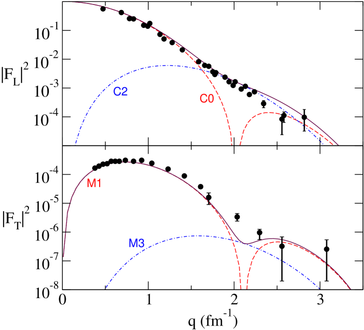
Figure 2: (Color online) The longitudinal and transverse form factors for scattering from the ground state of ¹⁰B. Data Hicks et al. (1988); Cichocki et al. (1995) are displayed by the filled circles.

These results for the longitudinal form factor concur in shape with those obtained Betker et al. (2005). However, we require no enhancement of the $C2$ term, as required by Betker et al. Betker et al. (2005), to achieve the good agreement with data. More noticeable though are differences we find in the transverse form factor results. In this we concur with the assessment made by Hicks et al. Hicks et al. (1988). These differences we attribute largely to changes wrought by considering a $(0+2)\hbar\omega$ model of the structure instead of the $0\hbar\omega$ model that was used by Betker et al. Betker et al. (2005).

III.1.2 Form factors for excitation of the $1^{+}$ and $3^{+}$ states

In Fig. 3, the longitudinal and transverse form factors from electron scattering to the $1^{+}$ and $3^{+}$ states in ¹⁰B are shown. The data Hicks et al. (1988); Cichocki et al. (1995) are displayed by filled circles with the longitudinal/transverse form factors shown in the top/bottom segments in this diagram. The data and results for excitation of the $1^{+}$ (0.718 MeV), the $1^{+}$ (2.154 MeV), and the $3^{+}$ (4.774 MeV) states are presented in the left, middle, and right panels respectively.

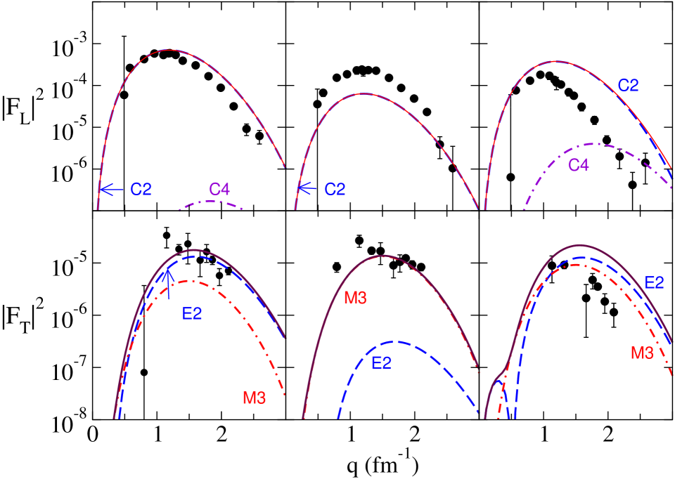
Figure 3: (Color online) The longitudinal (top) and transverse (bottom) form factors for electron scattering to the $1^{+}$ 0.718 MeV (left), the $1^{+}$ 2.154 MeV (middle), and the $3^{+}$ 4.774 MeV (right) states of ¹⁰B. Data Hicks et al. (1988); Cichocki et al. (1995) are displayed by the filled circles.

The solid curves are the total results being sums over the allowed multipole contributions. The longitudinal form factors all are dominated by the $C2$ components while $E2$ and $M3$ contributions are significant in the transverse form factor evaluations. The $C2$ and $E2$ contributions are displayed by the long dashed curves while the $M3$ values are shown by the dot-dashed lines. Cichocki et al. Cichocki et al. (1995) found similar results with their analysis of the longitudinal form factors though their $2\hbar\omega$ model results lay just under the data for both $1^{+}$ excitations. Our results for the longitudinal form factor for the $3^{+}$ 4.774 MeV state agree with that found previously Cichocki et al. (1995) but both calculations overestimate observation.

Our results for the transverse form factors are in good agreement with the data and are the result of mixtures of $E2$ and $M3$ multipole contributions predominantly. The $M1$ contributions to the 4.774 MeV results exist but are quite small, effecting small changes in values at low-$q$ values ($q\preceq 0.5$ fm^-1). We do not display it or its effect. Of note is that the $E2$ and $M3$ contributions are of similar size in the transverse form factors for the $1^{+}$ 0.718 MeV and $3^{+}$ 4.774 MeV cases, but the $M3$ is predominant in that form factor for scattering to the $1^{+}$ 2.154 MeV state.

As our calculated form factors for the $1^{+}$ 0.718 MeV state is larger than observation while that for the $1^{+}$ 2.154 MeV state is smaller, we considered a description for the two $1^{+}(T=0)$ states as a mix of those defined by our shell model (designated as $1^{+}_{1}$ and $1^{+}_{2}$ next) to be

$$\left|1^{+};0.718\right\rangle =C_{1}\left|1^{+}_{1}\right\rangle+\sqrt{1-C_{1}^{2}}\;\left|1^{+}_{2}\right\rangle$$

$$\left|1^{+};2.154\right\rangle =\sqrt{1-C_{1}^{2}}\;\left|1^{+}_{1}\right\rangle-C_{1}\left|1^{+}_{2}\right\rangle\ .$$ (14)

Varying the coefficients to define new sets of OBDME for the two longitudinal form factor evaluations then gave the results shown in the top panels of Fig. 4.

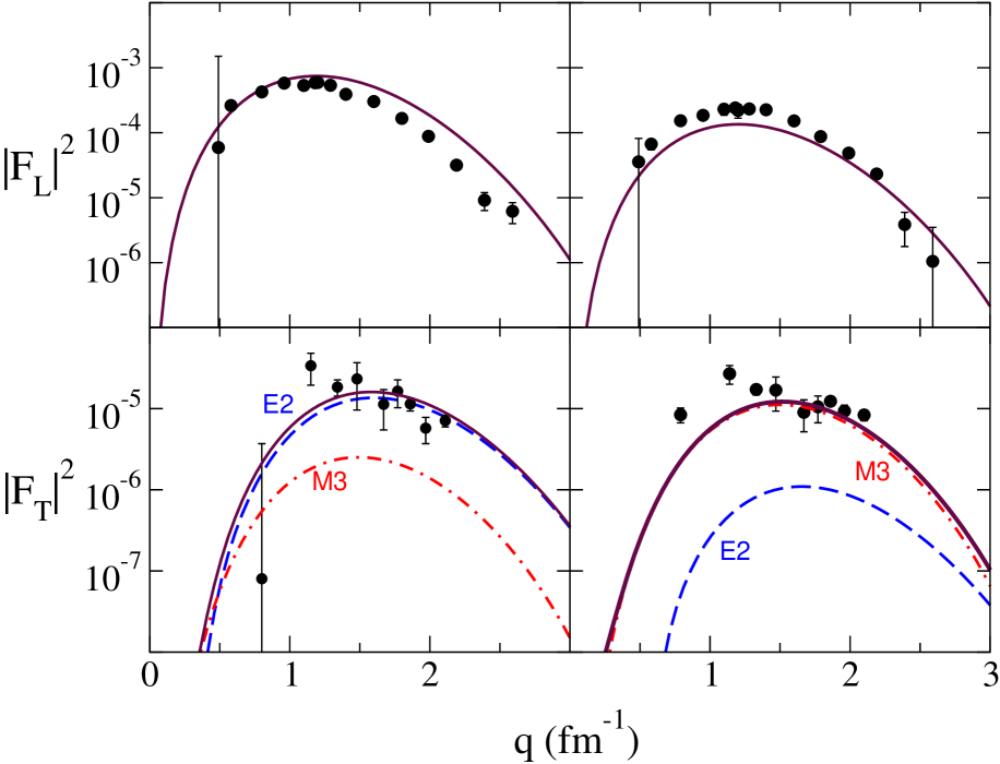
Figure 4: (Color online) The longitudinal (top) and transverse (bottom) form factors for electron scattering to the $1^{+}$ 0.718 MeV (left) and to the the $1^{+}$ 2.154 MeV (right) states in ¹⁰B. Results are those from the mixed shell model states.

The coefficient used was $C_{1}=0.99$ and the change in the form factor for the 2.154 MeV state seems dramatic but it must be remembered that the axes are linear-logarithmic. With that coefficient, the transverse form factors were then evaluated and the results are compared with the data in the bottom segments of the figure. The good agreement found previously has been retained with the (small) admixture states with only the balance between $E2$ and $M3$ contributions being changed.

The comparisons of results with transverse form factor data in these cases (isoscalar, even parity transitions) is the more remarkable since they are results of destructive interference between contributions involving the protons and the neutrons separately. Such is shown in Fig. 5.

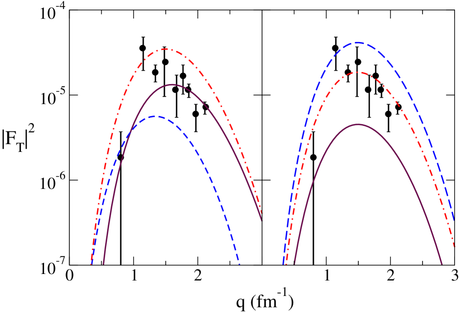
Figure 5: (Color online) The transverse form factors for electron scattering to the $1^{+}$ 0.718 MeV state of ¹⁰B showing the separate contributions from the protons (dashed line) and neutrons (dot-dashed line) in the target to the $E2$ (left) and $M3$ (right) multipolarities. The total transverse form factor for each multipolarity is shown by solid curves with the data again displayed by the filled circles.

Both the $E2$ (left) and $M3$ (right) proton and neutron component amplitudes destructively interfere to produce the final $E2$ and $M3$ form factors that are displayed by the solid curves. Thus relatively small variation in the structure description can have significant effects on these results. Nonetheless the final total result found using our $(0+2)\hbar\omega$ model prescription (the solid curve left lower diagram in Fig. 3), and in the left diagram of Fig. 4, is in quite good agreement with observation.

In Fig. 6 the form factors from electron scattering to the $2^{+}$ 3.587 MeV and $4^{+}$ 6.025 MeV states in ¹⁰B are displayed. The $2^{+}$ 3.587 MeV results are shown on the left and the longitudinal form factors are displayed in the top segments. Again the data Hicks et al. (1988); Cichocki et al. (1995) are displayed by the filled circles.

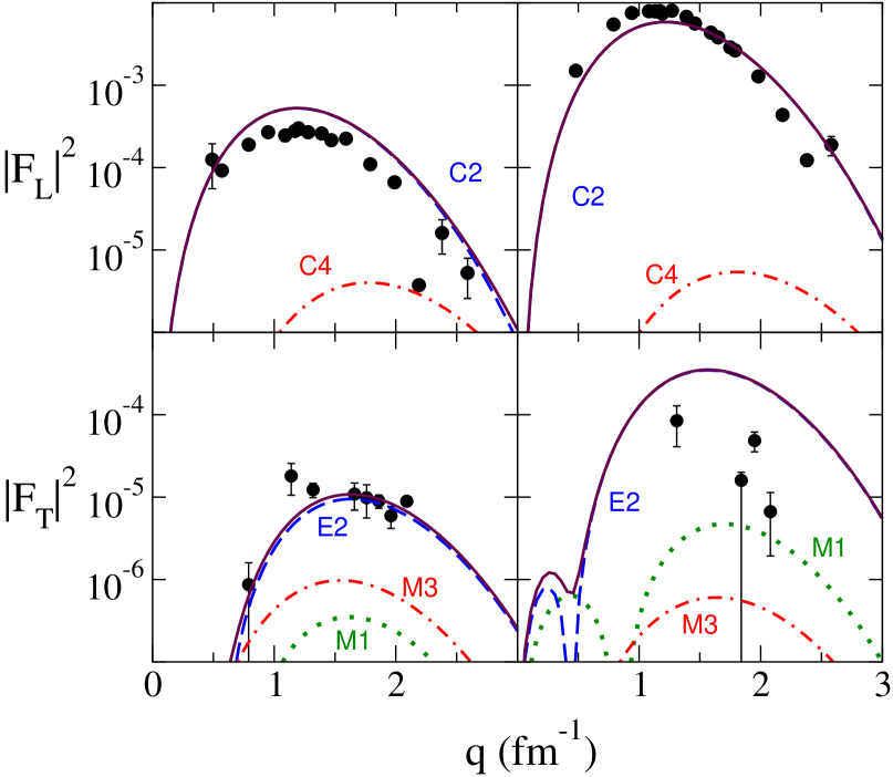
Figure 6: (Color online) The longitudinal (top) and transverse (bottom) form factors for electron scattering to the $2^{+}$ 3.587 MeV (left) and the $4^{+}$ 6.025 MeV (right) states of ¹⁰B.

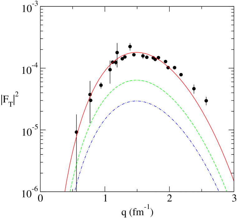
Figure 7: (Color online) The transverse form factor for the $0^{+};T=1$ 1.74 MeV state.

The longitudinal form factors are dominated by the $C2$ multipole transition and our model structure gives results in quite good agreement with both data sets. The small effect of the $C4$ term is shown in these plots. Our result for the $2^{+}$ transition agrees well with that found by Cichocki et al. Cichocki et al. (1995) but they required sizable core polarization additions to their model to fit the $4^{+}$ transition (longitudinal) form factor. None are needed with our model structure.

The transverse form factors for these two states shown in the bottom segments of Fig. 6, along with the separate multipole contributions. The results for the form factor of the $2^{+}$ 3.587 MeV state agrees quite well with the data while that for the $4^{+}$ 6.025 MeV overestimates the rather sparse data so far taken.

Finally we consider the form factor (purely transverse) measured with electron scattering to the $0^{+},T=1$ 1.74 MeV state in the ¹⁰B spectrum. This is the state we will consider as the analogue to the ground state of ¹⁰C which has been studied Wang et al. (1993) using the $(p,n)$ reaction on ¹⁰B. Form factors for this excitation are compared with data in Fig. 7. Therein the separate proton and neutron form factors are shown by the long dashed and dashed curves respectively, while their sum, constructive for this isovector transition, is depicted by the solid curve. The total result is in very good agreement with data (filled circles). This is also consistent with the observation Cichocki et al. (1995) that very little core polarization correction is needed to describe this isovector $M3$ transition. With our model of structure none is required.

III.2 Elastic scattering of 197 MeV protons

In Fig. 8 the evaluations of the cross section and analyzing power for elastic scattering of 197 MeV polarized protons are compared with the data Betker et al. (2005); the latter being displayed by the filled circles.

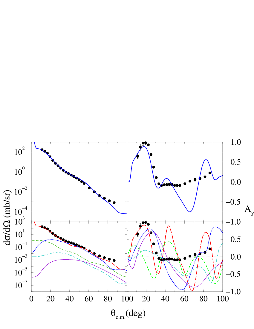
Figure 8: (Color online) The elastic scattering cross section (left) and analyzing power (right) from 197 MeV polarized proton elastic scattering from ¹⁰B. Complete results are compared with data (filled circles) in the top panels and component contributions are shown in the bottom panels. Details are given in the text.

In the top panels, the solid lines are the total calculated results which include contributions from all allowed multipoles. The individual multipole contributions are portrayed in the bottom panels by the long dashed lines for $I=0$, the dashed lines for $I=1$, the dotted curves for $I=2$, the dot-dashed curves for $I=3$, and the solid curves for $I=4$. Note each component analyzing power is that relative to the individual component cross section so their influence on the total analyzing power result is only proportionate to the multipole contribution to the cross section strength. As the effect of the $I=4$ amplitudes in the total cross section is very minor while the $I=0$ contribution is dominant for the forward angles, the latter is the dominating term in the total analyzing power and the former can be neglected. The other two allowed components, those for angular momentum transfer values $I=5$ and $I=6$ are much weaker and so are not displayed. Clearly the $I=2$ contributions become significant for scattering angles greater than 30^∘ so that the resultant cross section is in quite good agreement with the data Betker et al. (2005). The effect on the analyzing power is no less remarkable with a good representation now of the data to $\sim 50^{\circ}$. As with the phenomenological model analysis Betker et al. (2005), our results do not compare with the analyzing power data at larger scattering angles, but in that region the cross sections are less than 0.1 mb/sr. For such small values, with elastic scattering, the scattering model used may not suffice. Furthermore, as all components have large negative values of analyzing power in the vicinity of $60^{\circ}$ scattering angle, to match the data of essentially a null result requires that individual amplitudes destructively interfere. Small factors can influence the phases to effect such.

III.3 Inelastic scattering of 197 MeV protons

Betker et al. Betker et al. (2005) show cross-section and spin observable data from the inelastic scattering of 197 MeV polarized protons with ¹⁰B and for the same set of states for which we have analyzed electron scattering form factors. To analyze their data, we have used the DWA with distorted wave functions generated from the $g$-folding model of the optical potentials, the Melbourne force $g_{\text{eff}}$ used as the transition operator, and the nuclear state and transition details being those from the $(0+2)\hbar\omega$ shell model for ¹⁰B the same as used in the analyses of the electron scattering form factors. Consequently, each result shown hereafter was found with but one run of the DWBA98 code Raynal (1998). No a posteriori adjustments have been made to improve agreement with the data.

III.3.1 Cross sections and analyzing powers to the $1^{+}$ states

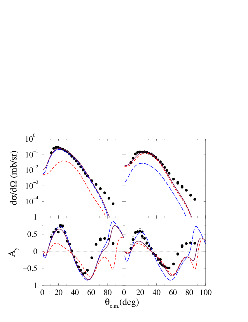
Figure 9: (Color online) The inelastic scattering cross section (top) and analyzing power (bottom) of 197 MeV polarized protons exciting the $1^{+}$ states of ¹⁰B. The data Betker et al. (2005) are compared to results as described in the text.

In Fig. 9 we show cross sections (top) and analyzing powers (bottom) for the excitation of the $1^{+}$ 0.718 MeV (left) and of the $1^{+}$ 2.154 MeV (right) states. The data, depicted by the filled circles, are compared with the results of our DWA calculations with the $I=2$ contributions depicted by the long dashed curves, the $I=3$ ones by the dashed curves, and our complete results by the solid curves.

Our cross section results are in quite good agreement with the data to $\sim 50^{\circ}$ scattering angle. Thereafter the calculated values decrease more rapidly than observation. However for the large scattering angles the data are less than $\sim 0.001$ mb/sr and are at least an order of magnitude smaller than the peak value. Small variations, most notably in the structure of the single-nucleon wave functions within the nuclear volume could account for that. The small admixture of the shell model states that gave such a dramatic improvement in comparisons of the electron scattering form factors, does little in these cases. As with the form factors for these states, the proton scatterings are mixes of scattering amplitudes for both $I=2$ and $I=3$ angular momentum transfers; the former dominant in the $1^{+}$ 0.718 MeV state excitation, the latter in the $1^{+}$ 2.154 MeV state case. Analyzing powers, being normalized by the cross sections, then also reflect the shape of the dominant components in those cross sections. In comparison with the data, the dominant $I=2$ character of the $1^{+}$ 0.718 MeV state excitation is very evident.

III.3.2 Excitation of the $3^{+}$ 4.774 MeV state

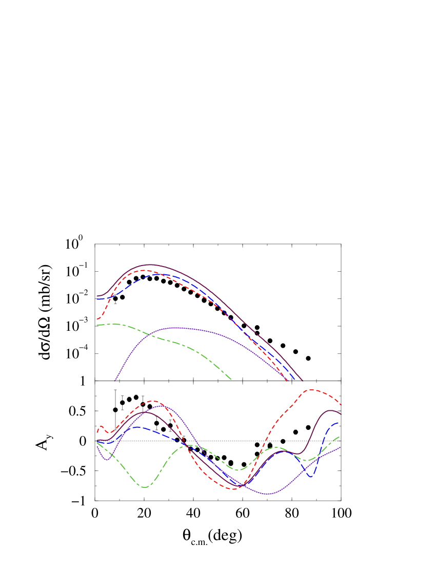
Figure 10: (Color online) The inelastic scattering cross section (top) and analyzing power (bottom) of 197 MeV polarized protons exciting the $3^{+};$ 4.774 MeV state of ¹⁰B.

The cross sections and analyzing powers for excitation of the $3^{+}$ 4.774 MeV state in ¹⁰B are shown in the top and bottom parts of Fig. 10 respectively. The data Betker et al. (2005) (filled circles) are compared to the DWA calculated results for purely an $I=2$ angular momentum transfer (dashed curves), for a purely $I=3$ case (long dashed curves) and for the full result (solid curves). The small $I=1$ and $I=4$ components are also displayed by the dot-dashed and dotted curves respectively. The allowed $I=0$ component is smaller than $10^{-4}$ mb/sr and so is not plotted.

The cross section is over predicted, as was the electron scattering form factor for this transition, and thus we need to improve the structure model description of this $3^{+}$ 4.774 MeV state. The shape of the calculated proton scattering cross section, however, is very similar to that of the data. This is quite different to what was found for the longitudinal form factor from electron scattering though the limited data of transverse form factor was reproduced. The latter though was dominantly a transition due to an M3 multipole. The analyzing power results show that the shape of the cross section has some significance as the components do sum to give a reasonable result.

III.3.3 Excitation of the $2^{+}$3.587 MeV and of the $4^{+}$ 6.025 MeV states

The inelastic scattering cross sections and analyzing powers from inelastic scattering of 197 MeV polarized protons exciting the $2^{+}$ 3.587 MeV and $4^{+}$ 6.025 MeV states in ¹⁰B are displayed in Fig. 11.

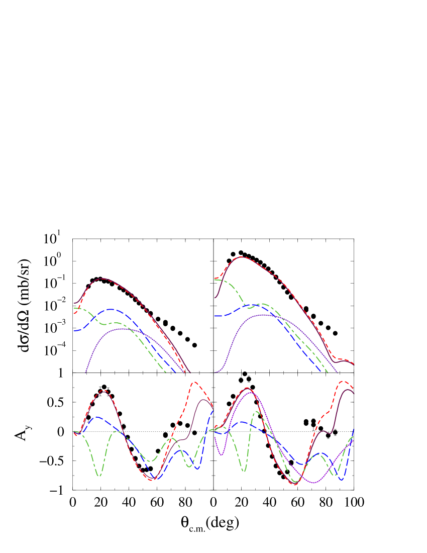
Figure 11: (Color online) The inelastic scattering cross section (top) and analyzing power (bottom) of 197 MeV polarized protons exciting the $2^{+}$ 3.587 MeV (left) and $4^{+}$ 6.025 MeV (right) states in ¹⁰B. The data Betker et al. (2005) (filled circles) are compared to the evaluations as described in the text.

The predictions are in good agreement with data, to $\sim 60^{\circ}$ for cross sections $\geq 10^{-3}$ mb/sr. The total results are portrayed by the solid lines and those for individual angular momentum transfer values are shown by the dot-dashed curves ($I=1$), by the dashed curves ($I=2$), by the long dashed curves ($I=3$), and by the dotted curves ($I=4$). Higher multipole contributions are not shown as they have peak values less than $10^{-5}$ mb/sr. These results mirror the fits to data that we found with the chosen structure for the electron scattering form factors in that the dominant contributions are of quadrupole type and in the quality of fit to cross section data to $\sim 3$ fm^-1 linear momentum transfer. The analyzing power data also are well reproduced at least to $\sim 50^{\circ}$.

III.3.4 Inelastic excitation of the $0^{+};T=1$ state and ($p,n$) scattering to its analogue

Finally, in Fig. 12, cross sections and analyzing powers from the 186 MeV $(p,n)$ reaction to the ground state $(0^{+};T=1)$ of ¹⁰C and from the inelastic scattering of 200 MeV protons to the isobaric analogue state (1.74 MeV) in ¹⁰B are shown. The OBDME for the inelastic scattering to the analogue scale to those for the charge exchange reaction by an isospin Clebsch-Gordan coefficient. Hence the cross sections for inelastic scattering to the 1.74 MeV $0^{+};T=1$ state of ¹⁰B depicted in Fig. 12 have been scaled by a factor of 2.

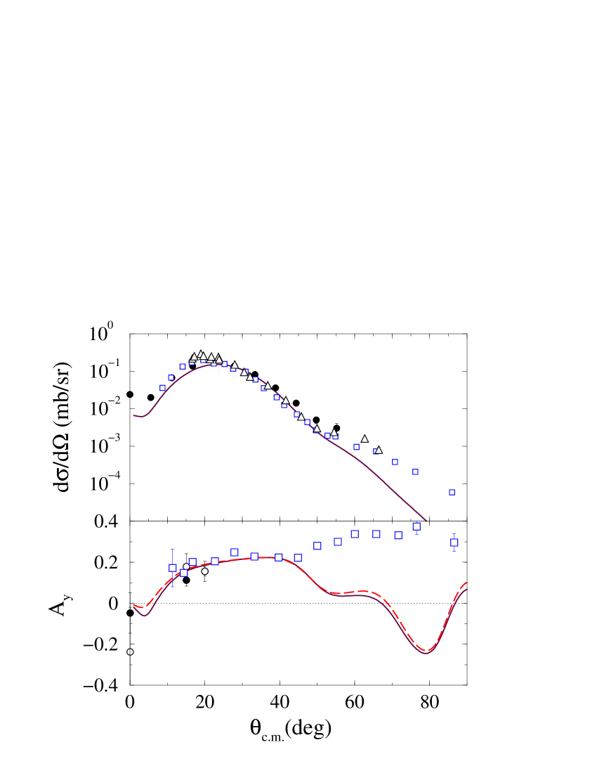
Figure 12: (Color online) Cross sections (top) and analyzing powers (bottom) from the 186 MeV $(p,n)$ reaction to the ground state $(0^{+};T=1)$ of ¹⁰C. Included are data, with cross section scaled by a factor of 2, from the inelastic scattering (of 200 MeV protons) to the isobaric analogue state (1.74 MeV) in ¹⁰B.

In this figure, the charge exchange data are depicted by the solid circles while the data from the inelastic scattering (of 200 MeV protons) to the isobaric analogue state are depicted by the open squares. The solid curves are the results we have obtained using our model of structure. For comparison, the dashed curve in the analyzing power segment is the result we found for the polarization in this (inelastic) transition. The differences between calculated spin measurables are trivial. In this case we have shown results and data taken to a scattering angle of 90^∘, and it is appropriate to view them in two parts; for scattering angles below and above $\sim 50^{\circ}$. At that boundary, the cross sections have values $\sim 10^{-3}$ mb/sr which is $\sim 1$% of the peak values. As with our results for the other transitions, for scattering angles to $50^{\circ}$, the predictions for both the cross sections and analyzing powers are in quite good agreement with data. Likewise, the calculated cross sections decrease too rapidly for the larger scattering angles. That mismatch makes meaningless consideration of what results for spin observables given that those are normalized by the cross section values. However, we stress that it is a small magnitude, larger momentum transfer, character of the processes that are in error. Such can reflect needed improvements in one or more of the internal radial wave functions, the higher momentum transfer properties of the effective $NN$ interaction, and/or the reaction mechanism specifics. But to pay most attention to these deficiencies is to let “the tail wag the dog”. We do predict the appropriate structures and magnitudes of the data to $\sim 50^{\circ}$ where the cross sections have their largest values. Consequently the dominant reaction mechanism and its details, including the choice of nuclear structure are credible.

III.4 Other spin observables

Additional to the analyzing powers (and polarizations), the spin observables of polarization transfer coefficients have been measured Betker et al. (2005); Baghaei et al. (1992); Wang et al. (1993). The data taken by Betker et al. Betker et al. (2005) from ¹⁰B (which has a ground state of spin-parity $3^{+}$), reasonably satisfy the conditions noted by Liu et al. Liu et al. (1996) and given in Eq. (13). Those are met for scattering from spin zero targets whence there should be only three independent coefficients. Nonetheless we have evaluated all five to see how well those links are satisfied by the assumed shell model spectroscopy.

III.4.1 The polarization coefficients, $D_{NN^{\prime}}$

In Fig. 13 the $D_{NN^{\prime}}$ from both the elastic and inelastic scattering (to the $(0^{+};T=1)$ 1.74 MeV state) of 197 MeV protons are shown. The elastic scattering data Betker et al. (2005) are depicted by the opaque, and the inelastic scattering data Baghaei et al. (1992) by the filled circles respectively.

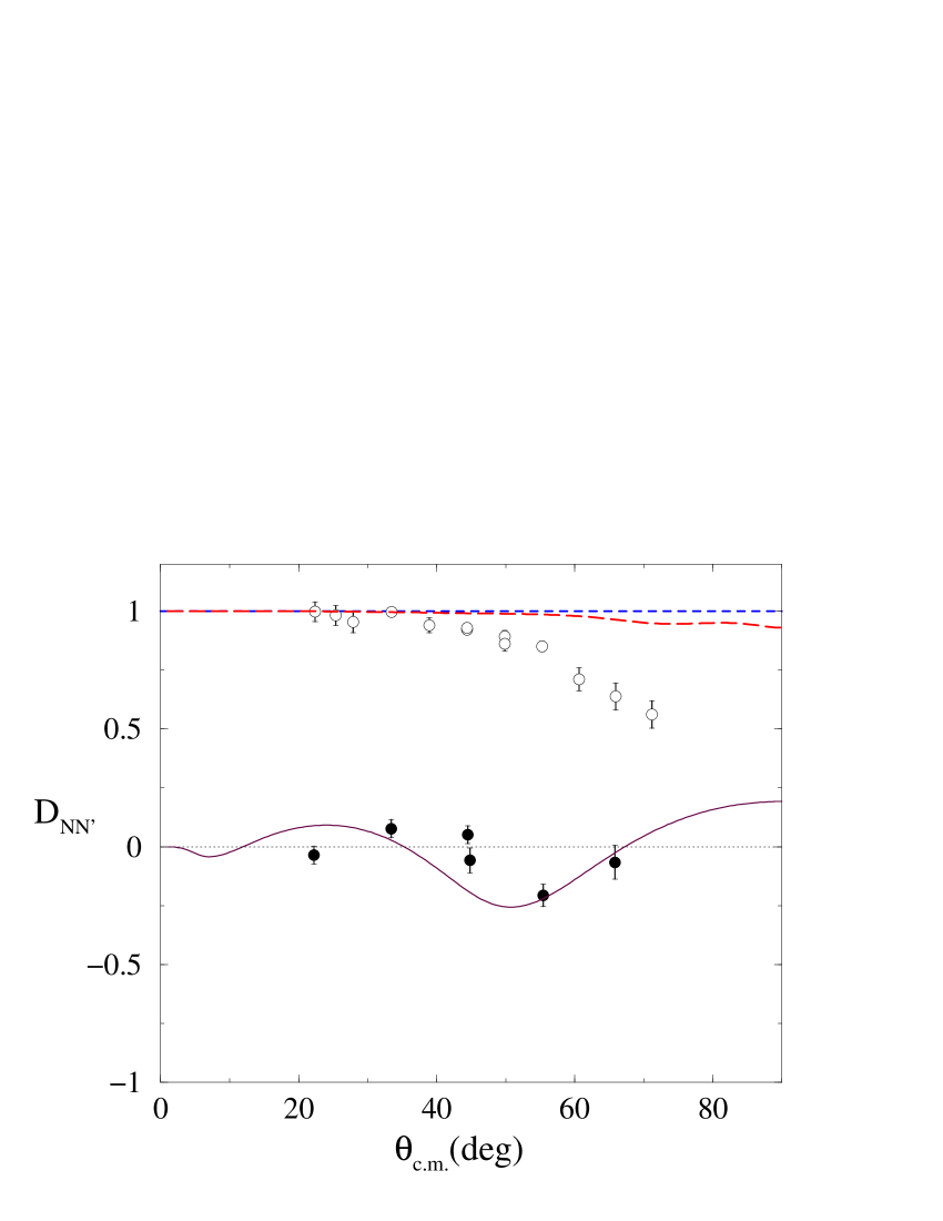
Figure 13: (Color online) Polarization transfer coefficients $D_{NN^{\prime}}$ from the elastic scattering of 197 MeV protons from ¹⁰B and from inelastic scattering to the $(0^{+};T=1)$ at 1.74 MeV.

The elastic scattering data are compared with calculated results for $I=0$ (dashed curve) and $I=2$ (long dashed curve) elastic scattering components. The inelastic result involves the unique $I=3$ transfer. These angular momentum transfer components dominate the transitions. The elastic scattering data are close to the value 1, as expected by the symmetry condition in Eq. 13, up to $\sim 40^{\circ}$. At larger scattering angles they decrease significantly. Our two results, for the pure multipoles, $D_{NN^{\prime}}^{(2)}$ and $D_{NN^{\prime}}^{(3)}$, as well as the total that can be formed by the summation,

$$D_{NN^{\prime}}=\frac{\sigma_{2}D_{NN^{\prime}}^{(2)}+\sigma_{3}D_{NN^{\prime}}^{(3)}}{[\sigma_{2}+\sigma_{3}]}\ ,$$ (15)

where $\sigma_{I}$ are the pure multipole ($I$) differential cross sections, deviate far less from 1 than the data. This effect is very similar to that found by Betker et al. Betker et al. (2005).

The $D_{NN^{\prime}}$ for the unnatural parity transition to the $0^{+};T=1$ 1.74 MeV state lies close to zero and our (pure $I=3$) result agrees quite well with the data Baghaei et al. (1992) shown by the filled circles. Though our effective interaction is a complicated mix of operator terms, it is preset for all calculations of all transitions and observables. It is medium dependent and so the improvement in results, noted Baghaei et al. (1992) by use of effective-mass approximations upon a phenomenological Franey-Love interaction, is confirmed as well as improved.

The $D_{NN^{\prime}}$ measured with the inelastic scattering to other states in ¹⁰B are compared with the results of our calculations in Fig. 14.

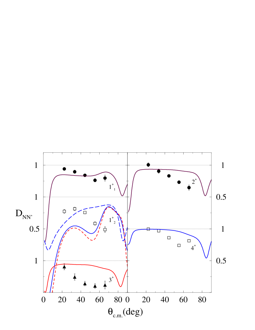
Figure 14: (Color online) Polarization transfer coefficients $D_{NN}$ from inelastic scattering of 197 MeV protons from ¹⁰B leading to the states identified by their values of $J^{\pi}$.

In this figure, the results shown in the left panel are from excitation of the $1^{+}$ 0.718 MeV state (top), from the excitation of the $1^{+}$ 2.15 MeV state (middle), and from the excitation of the $3^{+}$ 4.774 MeV state (bottom). In the right panel the results for excitation of the $2^{+}$ 3.59 MeV and of the $4^{+}$ 6.02 MeV states are depicted in the top and bottom parts respectively. The solid curves display the complete results when both $I=2$ and $I=3$ contributions dominate. The excitations of the $2^{+}$ and $4^{+}$ states are almost pure $I=2$. With the $1^{+}_{2}$ (2.15 MeV) results we also display the separate $I=2$ (long dashed curve) and $I=3$ (dashed curve) results. Clearly in this case the octupole is the more significant term. With the $1^{+}_{1}$ (0.718 MeV) transition the $I=2$ component is the more significant.

With the exception of our results for the $1^{+}_{2}$ excitation, these evaluated $D_{NN^{\prime}}$ resemble those found by Betker et al. Betker et al. (2005). The mix of $I=2$ and $I=3$ components in our shell model structure gives a good result but it does not do well for the $1^{+}_{2}$ transition. The small admixtures favored by the electron scattering form factor results little alters these findings. The comparison of results and data for the $3^{+}$ state excitation also is poor though it is to be remembered that the cross-section data for this transition also were overestimated. There is clearly a need for an improved description of the $3^{+}$ state.

III.4.2 The polarization transfer coefficients, $D_{LL^{\prime}}$, $D_{SS^{\prime}}$, $D_{LS^{\prime}}$, $D_{SL^{\prime}}$.

The dominant component contributions to the calculated coefficients, $D_{LL^{\prime}}$, and $D_{SS^{\prime}}$ are displayed in Fig. 15.

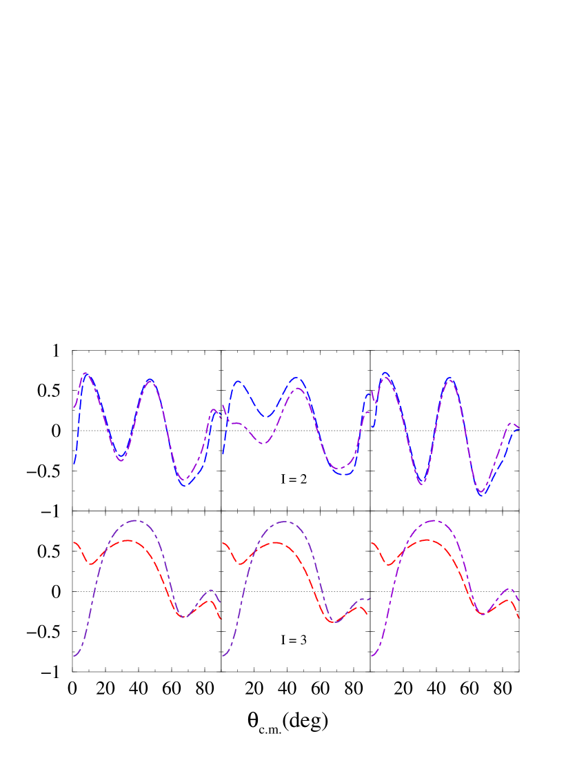
Figure 15: (Color online) Polarization transfer coefficients $D_{LL^{\prime}}$ (long dashed curves) and $D_{SS^{\prime}}$ (dot-dashed curves) for inelastic scattering of 197 MeV protons from ¹⁰B exciting the $1^{+}$ 0.718 MeV (left), $1^{+}$ 2.154 MeV (middle), and $3^{+}$ 4.774 MeV (right) states.

The top line of these diagrams contain the contributions for angular momentum transfer $I=2$ while the bottom line shows the results for $I=3$. From left to right the results are those for excitation of the $1^{+}_{1}$, the $1^{+}_{2}$, and the $3^{+}$ states respectively. As evident in the top panels, the $I=2$ components are very similar and largely in line with the symmetry conditions of Eq. (13). There are some divergence between the $D_{LL^{\prime}}$ and $D_{SS^{\prime}}$ with the $I=3$ components (shown in the bottom segments), however. Both have a positive peak at $\sim 40^{\circ}$, and a close agreement above $\sim 60^{\circ}$, but at forward scattering angles they are quite different.

For the same three states, and with specifics as given in Fig. 15, the component values of the polarization transfer observables $D_{LS^{\prime}}$ and $D_{SL^{\prime}}$ are depicted in Fig. 16

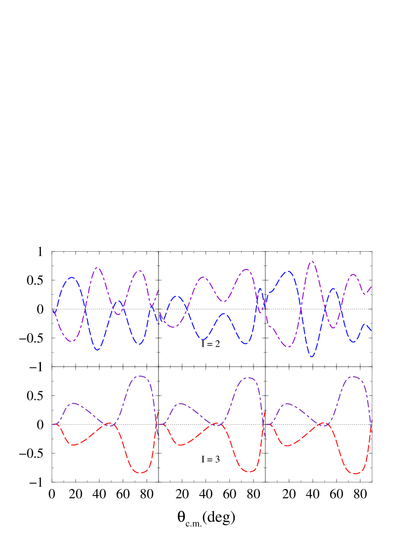
Figure 16: (Color online) Polarization transfer coefficients $D_{SL^{\prime}}$ (long dashed curves) and $D_{LS^{\prime}}$ (dot-dashed curves) for inelastic scattering of 197 MeV protons from ¹⁰B exciting the $1^{+}$ 0.718 MeV (left), $1^{+}$ 2.154 MeV (middle), and $3^{+}$ 4.774 MeV (right) states.

As with the $D_{NN^{\prime}}$ and $D_{SS^{\prime}}$, the $I=2$ and $I=3$ components for each state are markedly different in shape. However, for all three transitions the results are similar ($I=2$) and very similar ($I=3$) with differences among the latter being no more than a few percent. With these observables, and for both angular momentum transfer values, the mirror symmetry of the conditions of Eq. (13) is clear.

Then, in Fig. 17, the complete results for the spin observables $D_{LL^{\prime}},D_{SS^{\prime}}$, and $D_{LS^{\prime}}$ are compared with data Betker et al. (2005).

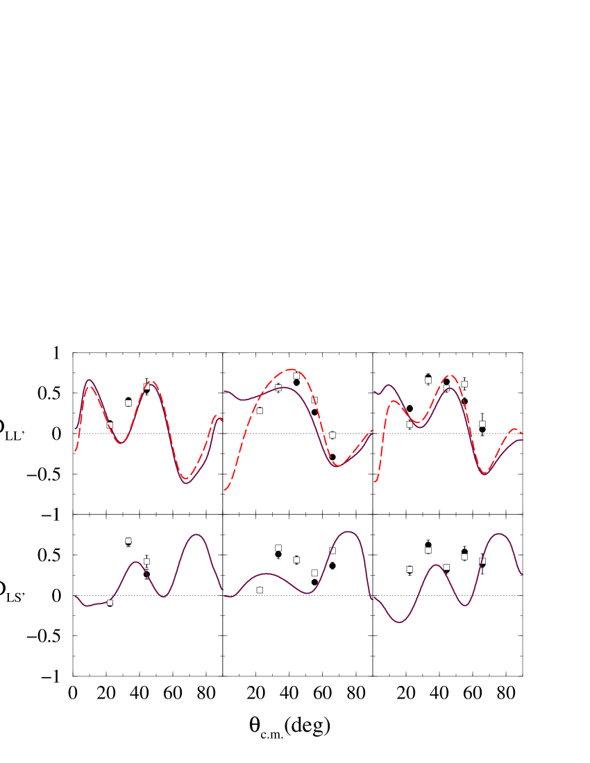
Figure 17: (Color online) Polarization transfer coefficients for inelastic scattering of 197 MeV protons from ¹⁰B exciting the $1^{+}$ 0.718 MeV (left), $1^{+}$ 2.154 MeV (middle), and $3^{+}$ 4.774 MeV (right) states. Other details are given in the text.

In the top segments, the solid and dashed curves show the calculated results for $D_{LL^{\prime}}$ and $D_{SS^{\prime}}$ respectively. The $D_{LL^{\prime}}$ data are displayed by the solid circles while those for $D_{SS^{\prime}}$ are given by the open squares. The solid curves in the figures shown in the bottom segments of this figure are the calculated $D_{LS^{\prime}}$ results (nearly identical to those for $-D_{SL^{\prime}}$). They are compared with data Betker et al. (2005) where the solid circles are the values for $D_{LS^{\prime}}$ and the open squares for $-D_{SL^{\prime}}$. Given that spin measurables are quite sensitive to details in the evaluations, these results agree quite well with the data from the three transitions.

Finally, in Fig. 18, we show the polarization transfer coefficients, $D_{LL^{\prime}}$ (top) and $D_{LS^{\prime}}$ for inelastic scattering of 197 MeV protons from ¹⁰B exciting the $2^{+}$ 3.59 MeV and the $4^{+}$ 6.02 MeV states.

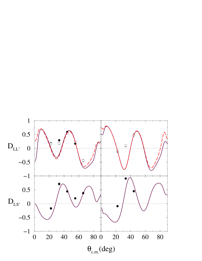
Figure 18: (Color online) Polarization transfer coefficients, $D_{LL^{\prime}}$ (top) and $D_{LS^{\prime}}$ bottom, for inelastic scattering of 197 MeV protons from ¹⁰B exciting the $2^{+}$ 3.59 MeV and the $4^{+}$ 6.02 MeV states. The results for those two states are shown in the left and right panels respectively.

These transitions are dominated by the $I=2$ contributions and our results (solid curves) agree very well with the limited data available. For comparison we show by the dashed curves, our results for the $D_{SS^{\prime}}$ coefficients. In both transitions the symmetry condition of Eq. (13) is well met.

IV Conclusions

We have made a comprehensive assessment of the structure of the ground and low excitation states in ¹⁰B. We have assumed that those states are described by wave functions determined from a no-core shell model calculation. The no-core shell model was defined within a complete $(0+2)\hbar\omega$ single particle space and the MK3W shell model interaction used to specify the Hamiltonian. A most striking feature of the results of that calculation was that the ground and first excited states are inverted. However, the splitting is but a few hundred keV, and with the “right” three-nucleon force that inversion was effected. Likewise static moments improved with those quantum Monte-Carlo calculations.

Nonetheless, we persist with the no-core shell model since only with its wave functions could we specify OBDME for use in fully microscopic model studies of electron and medium energy ($\sim 200$ MeV) proton scattering. The scattering calculations are predictions since all details required are predetermined in the relevant programs. Allowance for meson exchange current effects in electron scattering was made in the transverse electric form factors by recourse to Siegert’s theorem. The proton scattering calculations were made using a $g$-folding model for the optical potentials and a DWA for the inelastic processes. The electron scattering form factors (longitudinal, electric transverse, and magnetic transverse) found with the no-core shell model wave functions were in good agreement with observation requiring only small admixtures between the two shell model $1^{+}$ states in those transitions. Those $1^{+}$-state excitations however are especially sensitive as the neutron and proton amplitudes destructively interfere.

The shell model details were used to predict many observables from the scattering of 197 MeV polarized protons from ¹⁰B, for which there are much data. The elastic scattering observables were evaluated using the nonlocal optical potential formed by $g$-folding of the model wave functions with a complex, medium-dependent, effective $NN$ interaction. The resultant cross section matched data well as did the analyzing power, at least to momentum transfers for which the cross section exceeded $\sim 0.1$ mb/sr in size. Likewise on using a DWA, the cross sections from inelastic scattering to the low excitation states also matched data quite well at momentum transfer values for which those cross sections exceed $\sim 10^{-3}$ mb/sr. By and large so did spin observable results.

The quality of match between our predictions of these complementary scattering data involving the ground and low excitation states in ¹⁰B, is evidence that the wave functions for the nucleus obtained from the $(0+2)\hbar\omega$ shell model are quite reasonable descriptions of those states. The slight disparities in the calculated spectrum compared with the known one at low excitation (a few hundred keV) are due to missing elements in the shell model Hamiltonian, such as three-nucleon force effects. But their inclusion in the structure calculation should not seriously alter the eigenvectors. At best, the inclusion of such terms in the Hamiltonian should only give rise to small perturbations in the wave functions.