A Morphological Approach to the Pulsed Emission from Soft Gamma Repeaters

Abstract

We present a geometrical methodology to interpret the periodical light curves of Soft Gamma Repeaters based on the magnetar model and the numerical arithmetic of the three-dimensional magnetosphere model for the young pulsars. The hot plasma released by the star quake is trapped in the magnetosphere and photons are emitted tangent to the local magnetic field lines. The variety of radiation morphologies in the burst tails and the persistent stages could be well explained by the trapped fireballs on different sites inside the closed field lines. Furthermore, our numerical results suggests that the pulse profile evolution of SGR 1806-20 during the 27 December 2004 giant flare is due to a lateral drift of the emitting region in the magnetosphere.

1 Introduction

Soft Gamma Repeaters (SGRs) seemed weird since the first discovery on 1979 March 5 (Mazets et al., 1979) for their mysterious characteristics such as the large energy release, the repetitive emission of bursts in hard X-rays or soft gamma-rays bands, and the pulsed periodical emissions after the bursts and in the quiescent stages whose morphologies are both energy-dependent and time-dependent (see Woods & Thompson (2004) for a recent review). So far, the catalogue has four SGRs confirmed plus one candidate. SGRs are found to be associated with young ($\sim 10^{4}$ yr) supernova remnants (SNRs), and their spin periods are $5\sim 8\rm{s}$ and at a large spin down rate about $10^{-11}\rm{s~{}s^{-1}}$, which give an inferred ultra-strong dipolar magnetic field at the order of $10^{14}\sim 10^{15}\rm{G}$.

A variety of models were proposed to understand the physics of SGRs, and the magnetar model is now widely accepted to ascribe SGRs as neutron stars with magnetic field of $10^{14}\sim 10^{15}$G (Thompson & Duncan, 1995, 1996). Unlike most of the pulsars in the neutron star family powered by their spin-down, the high-luminosity bursts and the persistent X-ray or soft $\gamma$-ray pulsations of magnetars come from the decay of their ultra-strong magnetic fields. The spectrum of the persistent X-ray emission could be fitted by a superposition of a blackbody component and a power law, which suggests that besides the radiation from the neutron star surface, there is another component coming from the magnetosphere.

The high-luminous burst has now been successfully interpreted by the dissipation of magnetic energy. However, the persistent long-period pulsations in the quiescent X-ray emission of SGRs are still not well understood for their complicated and astonishing morphologies. Thompson, Lyutikov & Kulkarni (2002) assumed that the angular pattern of the X-ray flux are modified by the resonant cyclotron scattering at a distance about 50-100 km above the neutron star, and multi-pulses are generated by some effects associated with the twisted magnetosphere (e.g., the optical depth is thin near two magnetic poles, and thick at the magnetic equator). However, their numerical results from the Monte-Carlo simulation has a bias in favor of the orthogonal dipole (i.e., the magnetic axis is perpendicular to the spin axis), and the viewing angel has also to be nearly $90^{0}$ from the spin axis, for the photons escaping from optically thin poles (Fernández & Thompson, 2007). In addition, the separation of the strong peaks in their calculations is always $\pi$ (half phase cycle), which differs from the observation. Thompson (private communication, 2005) agreed that the change in the persistent pulse profile reflects a re-distribution of persistent currents on closed field lines. However, he ascribed such re-distribution as the gradual change in the magnetic twist at a distance of 30-100 km, while our understanding for that is due to the gradual migration of the emitting regions (crustal platelet motion or hot plasma drifting in the magnetosphere, we will discuss the possibility of each candidate in §4).

In this paper, we present some simulated pulsed profiles by assuming the radiation region located in the closed field lines, and make attempts to simulate the radiation morphology evolution in one particular event, i.e., SGR 1806-20 burst on 27 December 2004. We first have a general review on the timing properties of SGRs in §2. In §3, we present the motivation to reproduce the light curves in the closed field lines and the resultant profiles. In §4, we applied the geometrical model to the well-known December 2004 burst of SGR 1806-20 and calculate the radiation morphology by a three-dimensional magnetosphere simulation. We also try to explain the change in the persistent pulse profile. A brief discussion is given in §5.

2 Periodical Emissions from SGRs

The periodical emissions of the four confirmed SGRs have been detected in the decay of burst and the quiescent or persistent stages, with the periods in the 5-8 seconds range which are the spin periods of the neutron stars. The pulse profiles show many interesting and even surprising morphologies, some of which are totally different from the canonical radio or high energy pulsars. The characteristics of light curves of the X-ray and $\gamma$-ray pulsars such as number of peaks, the peak separation and the relative amplitudes of the peaks are unchangeable, while those of the SGRs are time dependent. Here, we list several main features of the persistent emissions from SGRs:

1. Multi-peaked morphology: The most dramatic example is the pulse profile change of SGR 1900+14 after the outburst on 1998 August 27. A four-peaked repetitive pattern of the X-ray light curve was detected by both Ulysses and BeppoSAX half a minute after the burst onset (Hurley et al., 1999; Feroci et al., 2001), and these peaks were found to be evenly spaced at 1.0 s intervals on the 5.16 s rotation period. And several minutes later, this multi-peaked profile evolved as a simple sinusoidal morphology(Woods & Thompson, 2004), and this evolution in pulse profile lasted for a couple of years. Such change in morphology is also found in the RXTE PCA archive of SGR 1806-20 between 1996 and 2005(Woods et al., 2007). During the 10-year observation, the 2-10 keV pulse shape evolved from one broad peak pattern to a three-peaked one in 2003, and then the sinusoidal shape again until the multi-peaked profile after the burst on December 2004 (see Fig. 3 in Woods et al. (2007)).

2. Relative magnitudes of peaks: Besides the evolution of the number of peaks, the relative magnitudes of the peaks in one phase cycle also change with time. Palmer et al. (2005) showed such pulse profile evolution during the giant flare of 27 December 2004. The folded light curves in different time intervals from 30 to 265 seconds following the main spike indicate the growth of the second peak, whose intensity related to the primary peak increases from the DC level to nearly equal in height. In the other words, we can say that the primary peak fades until the same magnitude as the secondary one. At the late stage of the decay of the giant flare, the relative magnitude of the third peak 0.2 in phase prior to the primary one starts to grow up.

3. Energy-dependent profiles: The evolution of pulse profiles of SGRs is not only time-dependent, but also changes in different energy bands. Woods et al. (2007) investigated the energy dependence of the SGR 1806-20 pulse profiles in three energy bands between 2 to 40 keV. Six months before the flare, there was only one broad peak in the pulse profile below 15 keV, and it showed two clear peaks in the 15-40 keV band. After the giant flare, the light curve became more complicated, showing multiple peaks in all energy intervals, and the peaks were inconsistent in phase (see Fig. 4 in Woods et al. (2007)).

The totally different phenomena require the totally different physics in this small (may be not small) group of neutron stars, compared with the canonical pulsars. The thermal spectrum component suggests that the radiation partly comes from the hot spots on the stellar surface. In addition, the phase inconsistence of the pulse profile indicates that it may not be localized in a particular region, and the non-predictable star quakes can produce the randomly-localized emitting regions during every burst event. This is the main motivation for us to build up the model of the alterable pulse profiles in the next section.

3 Radiations from the Closed Field lines

3.1 Why closed regions?

The theoretical models for radiation from high energy pulsars (e.g. Crab and Vela) require that the radiation engine is located in the open field line region no matter in the polar gap model (Harding, 1981; Daugherty & Harding, 1996), or the outer gap model (Cheng, Ho & Ruderman, 1986; Chiang & Romani, 1994; Romani & Yadigaroglu, 1995; Cheng, Ruderman & Zhang, 2000), or the modified outer gap model (Dyks & Rudak, 2003; Jia et al., 2007). However, we cannot apply them to magnetars to explain their persistent X-ray emissions. We assume that the pulsed emissions of SGRs in the decay or afterglow of the bursts are originated in the closed regions rather than in the open regions. We have three main reasons for confining the radiation regions to the closed zones in the neutron star magnetosphere:

1. The volume occupied by the open field lines is much smaller compared to that by the closed field lines. Take SGR 1806-20 for example, the spin period is $P=7.56~{}\rm{s}$, which means the radius of the light cylinder reaches $R_{L}=\frac{cP}{2\pi}=3.6\times 10^{10}~{}\rm{cm}$, where $c$ is the speed of light. Thus, the radius of the polar cap is $R_{p}=R_{\ast}\sqrt{R_{\ast}/R_{L}}=5.3\times 10^{3}~{}\rm{cm}$, corresponding to an angular size of $\theta_{p}=0.3^{0}$, much smaller than the characteristic size of the crustal platelet, where $R_{\ast}=10^{6}~{}\rm{cm}$ is the stellar radius. So, the polar cap area is only $10^{-5}$ of the neutron star surface, and there is no reason why the crustal platelet, where the magnetic energy is released, should be located in the open area.

2. The open field lines reach the light cylinder, where the co-rotating speed approaches the speed of light, and the relativistic effects play a significant role in the radiation morphology (Romani & Yadigaroglu, 1995). Such effects lead to the sharp and narrow peaks of the light curves, and both peaks are produced by one single pole. However, those effects become less important when it is applied to the closed field lines, for they are much closer to the stellar surface than the open lines. As shown in Fig.1, we find that the farthest distance where the closed field lines can reach drops much quickly when their footprints are displaced further away from the polar cap. For the closed line on the plane (on which both the magnetic axis and spin axis lie) with layer parameter $a_{1}=5$, it only reaches a distance less than $0.05R_{L}$ away from the stellar surface, and $0.01R_{L}$ for $a_{1}=10$ (the definition of $a_{1}$ is given in §3.2). Thus, the double-peaked profiles are not necessary for closed field lines, and the broad peak could be a general product instead of the sharp one. Other features, like the peak separation and the multi-peaks, could also be explained by the closed field lines (details to be discussed in the next section).

3. The emitting region has not to be localized on some particular sites on neutron star surface or inside the magnetosphere while in the open field lines, the accelerating gap is restricted to the null charge surface (Goldreich & Julian, 1969; Cheng, Ruderman & Zhang, 2000). This freedom in loci ensures the variety of the pulse profiles during different outbursts, for we can argue that time-dependent light curves result from different bunches of magnetic field lines where the plasma is trapped.

3.2 Strategies for numerical simulation

Since we argue that the periodic pulsed radiation of magnetars in the quiescent state is released from the closed field line regions rather than the open one, we could apply the 3D magnetosphere model (Cheng, Ruderman & Zhang, 2000) to simulate the pulse profiles. The boundary of these two different regions is defined as a bunch of so called the last closed or the first open magnetic field lines, which are tangential to the light cylinder. The hot plasma is trapped in the closed region and oscillates along the closed field lines, and photons are assumed to be emitted outwardly along the tangential direction of the magnetic field lines, which makes the pulsed radiation much different from the one generated in the open area. In order to be consistent with the pulsar magnetosphere calculation in the high-energy pulsar models, we adopted the same definition for the coordinates of footprints of the magnetic field lines and layer parameters(Cheng, Ruderman & Zhang, 2000). The shape of the polar cap could be determined by the footprints of the last closed field lines anchored in the stellar surface, and we can label the coordinates of these footprints as $(x_{0},y_{0},z_{0})$. Then we are able to define another set of footprints of magnetic field lines $(x^{{}^{\prime}}_{0},y^{{}^{\prime}}_{0},z^{{}^{\prime}}_{0})$ by multiplying a factor $a_{1}$ called layer parameter: $x^{{}^{\prime}}_{0}=a_{1}x_{0}$, $y^{{}^{\prime}}_{0}=a_{1}y_{0}$, and $z^{{}^{\prime}}_{0}=\sqrt{1-(x^{{}^{\prime}2}_{0}+y^{{}^{\prime}2}_{0})}$, where $a_{1}>1$ indicates the closed region, and $a_{1}<1$ represents the open ones.

Since the magnetosphere is co-rotating with the neutron star, aberration effect occurs along the line of sight. Thus, we have the aberrated emission direction (in the observer’s frame) $\mathbb{u}^{{}^{\prime}}=(u^{{}^{\prime}}_{r},u^{{}^{\prime}}_{\theta},u^{{}^{\prime}}_{\phi})$ in the expression of the direction $\mathbb{u}=(u_{r},u_{\theta},u_{\phi})$ in the co-rotating frame and the rotational speed $\beta=|\mathbb{r}\times\mathbb{\Omega}|/c$:

$$u^{{}^{\prime}}_{r} = \frac{u_{r}\sqrt{1-\beta^{2}}}{(1+\beta u_{\phi}c)}$$

$$u^{{}^{\prime}}_{\theta} = \frac{u_{\theta}\sqrt{1-\beta^{2}}}{(1+\beta u_{\phi}c)}$$

$$u^{{}^{\prime}}_{\phi} = \frac{u_{\phi}+\beta c}{(1+\beta u_{\phi}c)}.$$ (1)

Another effect taken into account is the time of flight, which differs a lot for the photons originated at different sites inside the magnetosphere. This effect can lead to the phase difference of the arrival photons comparable to the light curve period. Combing these two effects, and choosing the rotational axis as the $z$-axis, we obtain the phase angle $\Phi$ and the polar angle $\zeta$ given by (Yadigaroglu, 1997)

$$\cos\zeta = u^{{}^{\prime}}_{z}/u^{{}^{\prime}},$$

$$\Phi = -\phi^{{}^{\prime}}_{u^{{}^{\prime}}}-\mathbb{r}\cdot\hat{u}^{{}^{\prime}}/R_{L},$$ (2)

where $\phi^{{}^{\prime}}_{u^{{}^{\prime}}}=\arccos(u^{{}^{\prime}}_{x}/u^{{}^{\prime}}_{xy})$ (here $(x,y,z)$ is the cartesian coordinate system) is the azimuthal angle in the observer’s frame. Choosing $\Omega$-$\mu$ plane to be the $x$-$z$ plane, $u_{xy}^{\prime}$ is the length of the projection of $\hat{u}^{\prime}$ on the $x$-$y$ plane.

3.3 Simulated light curve profiles

In the following, we adopt in this paper the magnetic coordinates ($\theta_{\ast},\phi_{\ast}$) to describe the loci of radiation regions in the magnetosphere. The polar angle $\theta_{\ast}$ is defined as the angle with respect to the magnetic axis, instead of the rotational axis. The emitting region is assumed to be in the shape of a band along the azimuthal direction, with a relatively smaller longitudinal thickness compared with its azimuthal width. As the neutron star is rapidly rotating, we set the phase of the $\Omega$-$\mu$ plane defined by the rotational axis and magnetic axis as $\phi_{\ast}=0^{0}$. Therefore, the transverse extension of the emitting region along the azimuthal direction could be expressed as $\Delta\phi_{\ast}$, which is treated as a parameter in our numerical simulations in this paper. However, there is no particular parameter for a quantitative longitudinal thickness $\Delta\theta_{\ast}$ in our simulation, and we represent it by the layer parameter $a_{1}$, instead.

Combining those factors mentioned above, we show in Fig.2 and 3 two typical light curves generated in the closed field line zone. Fig.2 is a single sinusoidal pattern, and Fig.3 is a double-peaked morphology without any off-pulse phase. The spin period of SGR 1806-20 is applied in the calculation, and the inclination angle and viewing angle w.r.t. the spin axis are chosen to be $30^{0}~{}\rm{and}~{}50^{0}$. Both pulse profiles are commonly detected in the SGRs timing observations (e.g. Woods et al. (2007)). The azimuthal widths of the emission regions for these two cases are $\Delta\phi_{\ast}=180^{0}$, and the other parameters for these two plots, like $a_{1}$ and the ($\theta_{\ast},\phi_{\ast}$) coordinates of the emitting regions, are given in Table.1. In the upper panels of both figures, we show the emission projections onto the $(\zeta,\Phi)$-plane to illustrate the two kinds of light curves, respectively. We can find that the whole $(\zeta,\Phi)$-plane is fully filled by the emissions from closed field lines, compared with those partially-filled by the outer gap in the open lines (e.g. Fig.6-8 in Cheng, Ruderman & Zhang (2000)). The emission projection of Fig.3 has a dense bundle in the phase range (0.5, 0.7), which produces the secondary peak of the double-peaked light curve.

What makes such difference between these two kinds of light curves? As shown by Cheng, Ruderman & Zhang (2000), the neutron star rotation results in a non-uniform distribution of the magnetic field lines in the magnetosphere, i.e., the magnetic field lines are swept back to accumulate around the $\Omega$-$\mu$ plane. In our calculation, the only different parameter in both cases is the longitude of the emitting region. On the side around $\phi_{\ast}=0^{0}$, the accumulated field lines produce the one-peak dominated light curve profile (e.g. the single sinusoidal pattern), while on the other side around $\phi_{\ast}=180^{0}$, the widely-separated field lines make the double-peaked profile possible.

4 Application to SGR 1806-20 in December 2004

4.1 Pulse profile evolution

As illustrated in the standard magnetar model, the crust of the magnetar breaks when the magnetostatic equilibrium in the lower crust is no longer be sustained, and launches a hot fireball, which triggers the outburst of SGRs. The released energy comes from the reconnection of magnetic field lines in a crustal plate, which can be modelled as

$$E=\frac{B^{2}}{8\pi}l^{3},$$ (3)

where $B$ is the magnetic field in the crust, and $l$ is the size of the crustal plate. The energy released by SGR 1806-20 in the Dec 27 2004 burst is estimated to be as high as $\sim 10^{46}$erg, and by substituting the inferred magnetic field strength of order $10^{15}~{}\rm{G}$, we can estimate $l\sim 10^{5}~{}\rm{cm}$, which is about the thickness of the neutron star crust. A clump of electron-positron or electron-proton plasma is then ejected into the magnetosphere, and trapped by the magnetic field lines anchored in such crustal platelet. The charged particles emitted by the hot plasma travel along the closed magnetic field lines, and radiate photons. In the following emission morphology simulation, we will assume the emissivity along the field lines is uniform. However, the emission region along the azimuthal and polar directions have a finite characteristic dimension corresponding to $\sim 10^{5}$cm. We assumed that either the crustal motion driven by the neutron vortex (Ruderman, 1991) or the lateral motion of the plasma across the field lines driven by the residual electric field, could lead to the change of the radiation morphologies. We will discuss which mechanism is more plausible later.

We attempted to simulate the pulse profile evolution during the giant flare of 27 December 2004 (e.g. Figure 2 in Palmer et al. (2005)). The most significant feature of the SGR 1806-20 pulsed radiation is the increased amplitude of the secondary peak related to the primary one. Our trials on the numerical simulation suggest that such change is due to the motion of emitting region. We present our results in Fig.4, which shows the effect of the azimuthal motion of the emitting region across the magnetic field lines with the typical layer parameter $a_{1}=10$, anchored in the crustal plate with the size about $1.5\times 10^{5}$ cm. Fig.4 also shows some other features (e.g. the width of the peaks and the phase separation between two peaks) to be consistent with the observation. The inclination angle of the magnetic dipole and the viewing angle of the observer are chosen to be $30^{0}$ and $50^{0}$, respectively. We assume that size of the plasma or the emitting region remains unchanged during the motion, and we describe the loci of the emitting region center in terms of the $(\theta_{\ast c},\phi_{\ast c})$, which are the magnetic coordinates of the middle point of the emitting region at the typical layer. Since the motion is along the azimuthal direction, $\theta_{\ast c}=a_{1}\times\theta_{p}=3^{0}$ for all three panels in Fig.4. As the $\Omega$-$\mu$ plane is defined as $\phi_{\ast}=0^{0}$, the azimuthal angle $\phi_{\ast}$ increases along the spin direction of the neutron star. The center of the radiation region was shifted from $\phi_{\ast c}=-11^{0}$ (panel a in Fig.4) to $\phi_{\ast c}=0^{0}$ (panel b in Fig.4), and finally at $\phi_{\ast c}=7.5^{0}$ (panel c in Fig.4) All parameters applied in our model fitting are listed in Table.1.

As shown by Arendt & Eilek (1998), the polar cap of a rotating neutron star is asymmetrical and even probably discontinuous, which could make the radiation morphology complicated and asymmetrical. In our simulation, the primary peak at phase 0.9 of the light curve results from the majority of the magnetic field lines in which the plasma is trapped, and only a small portion of the field lines on the right edge of the plasma generate the secondary peak (at phase 1.2), where ’right’ means the site whose $\phi_{\ast}$ value is larger. As the plasma is drifted from left to right (along the direction $\phi_{\ast}$ increases), more magnetic field lines at the right site are enrolled to radiate photons, which makes the secondary peak grow up. The radial distance of the local place where the arrival photons are generated is shown in Fig.6. Since the magnetosphere co-rotates with the neutron star, we calculate the modelling velocity of the emitting region motion in $\phi_{\ast}$ direction. As shown in Fig.7, the speed of the drift is estimated to be $\sim 10^{4}~{}\rm{cm~{}s^{-1}}$ according to the pulse profile evolution timing by observation. We also give the expected radiation from the two magnetic poles in panel c of Fig. 4, which are indicated by two arrows. As the definition of the $(\Omega,\mu)$-plane, the magnetic poles are located at $\phi_{\ast}=0~{}\rm{and}~{}\pi$ (0 and 0.5 in the phase cycle), respectively. However, the time of flight effect makes the radiation from magnetic poles has a tiny shift in phase, e.g. 0.1 and 0.6. At the early stage, the flux of the radiation from the trapped plasma is so strong that the emissions from the polar caps could not be resolved. However, as the intensity of the two main peaks fades, the two minor peaks might become discriminable.

In general, the emitting region should not always move in one direction. Fig. 5 shows the pulse profile evolution when the motion of the radiation region is changed to be along the $\theta$-direction. Panel c is the same as the one in Fig. 4, and the light curve of panel d is produced when the center of plasma is located at $a_{1}$=20, with the same azimuthal position as that in panel c. We find that the morphology of the pulsed emission remains roughly unchanged, corresponds to the late stage ($\sim$ 170s after the burst) of tail in the giant flare of 27 December 2004. We want to remark that the light curve can also remain unchanged when the motion of the radiation region stops. We cannot differentiate these two possibilities from the light curve evolution.

4.2 Interpretation of numerical results

In order to simulate the time evolution of the light curves of SGR 1806-20, we have assumed that the emitting region can migrate in the magnetosphere. In the following, we would like to discuss several possible movements induced in the crust and the magnetosphere, and their resultant speeds.

The interaction between the flux tubes and vortex lines in the core of neutron star make them inter-pin to each other. The vortex lines will move out of the core due to the spin-down of the star, they drag the flux tubes with them. However, the flux tubes are anchored in the crust, consequently a large stress will be applied to the crust from the flux tubes (e.g. Ruderman 1991). When the crust breaks, the flux tubes will try to reduce their tension and drag the broken crust platelet to move. The maximum shear stress on the base of the crust from core magnetic flux tube motion which the crust could sustain is

$$S\sim\frac{BB_{crit}}{8\pi}\sim 3\times 10^{29}~{}\rm{dyn~{}cm^{-2}},$$ (4)

where $B_{crit}\sim 10^{16}~{}\rm{G}$ is the critical magnetic field inside the magnetic flux tube. However, the crust may already break before the magnetic stress reaches the maximum value. The shear modulus $\mu$ of a 1 km thick crust could not be larger than $10^{30}~{}\rm{dyn~{}cm^{-2}}$, and the crust may break when the stress reaches

$$S_{break}\sim f\mu\theta_{max},$$ (5)

where $f$ is a factor of order unity, and $\theta_{max}$ is the yield strain under tension or compression, which is $\sim 10^{-1}-10^{-3}$ (c.f. Ruderman 1991).

Another mechanism to drive the crust to move is the vortex creeping. As the rotation of the neutron star slows down, the flux tubes are driven outwardly by the the neutron vortices. The force acting on unit length of a flux tube at the core-crustal interface is (Chau, Cheng & Ding, 1992; Ding, Cheng & Chau, 1993)

$$f_{n}=\frac{2\Phi_{0}\rho_{c}R_{c}\Omega_{s}\omega_{cr}}{B_{c}},$$ (6)

where $\Phi_{0}=hc/2e\sim 2\times 10^{-7}\rm{G/cm^{2}}$ is the flux quantum, and the subscript $c$ represents the values in the core. $\Omega_{s}$ is the rotation rate of the core superfluid, and can be approximated as that of the crust $\Omega_{c}$ or the spin rate of the star in our following estimation. $\omega_{cr}$ is the maximum angular velocity lag between $\Omega_{s}$ and $\Omega_{c}$. $B_{c}$ is the core magnetic field, and could be only about $10^{-3}$ of the surface value because the flux tubes are pushed out of the core due to spin-down (Ding, Cheng & Chau 1993). Thus, we can estimate the total magnitude of the force acting on the crust platelet with area $A$. The number of flux tubes anchored in this platelet is given by

$$N_{f} = N_{total}\frac{A}{\pi R^{2}_{c}}$$ (7)

$$= \frac{A}{\pi R^{2}_{c}}\frac{\pi R^{2}_{c}B_{c}}{\Phi_{0}}=\frac{AB_{c}}{\Phi_{0}},$$

Substituting $f_{n}$ in Eq.6, we have the total driving force on a platelet

$$F_{n}=N_{f}f_{n}R_{c}=2A\rho_{c}R^{2}_{c}\Omega_{s}\omega_{cr}.$$ (8)

We then make a dimension analysis to estimate the velocity

$$<v>\sim\sqrt{F/\rho A}=(R^{2}_{c}\Omega_{s}\omega_{cr})^{1/2}.$$ (9)

$\omega_{cr}$ is given by various models as of order $10^{-6}~{}\rm{rad~{}s^{-1}}$ (Chau, Cheng & Ding, 1992), therefore, we have the velocity of the flux tube about $10^{3}~{}\rm{cm~{}s^{-1}}$.

However, when the flux tubes move, they will experience a drag force by the electron sea in the core. The drag force per unit length of a single flux tube is given by

$$f_{v}(v_{p})=\frac{3\pi}{64}\frac{n_{e}e^{2}\Phi^{2}_{0}v_{p}}{E_{f}\Lambda c}.$$ (10)

Here, $n_{e}\sim 10^{37}~{}\rm{cm^{-3}}$ is the electron density, and $E_{f}$ is the electron Fermi energy, which is about 100 MeV. The penetration length of a proton $\Lambda$ is $\sim 100~{}\rm{fm}$, and $v_{p}$ the velocity of the flux tube. By equating the vortex acting force $f_{n}$ and drag force $f_{v}$, we calculate the velocity as

$$v_{p} = \frac{64}{3\pi}\frac{E_{f}\Lambda c\rho_{c}R_{c}\Omega_{s}\omega_{cr}}{B_{c}n_{e}e^{2}\Phi_{0}}$$ (11)

$$\approx 10^{-12}~{}\rm{cm~{}s^{-1}},$$

and Ruderman, Zhu & Chen (1998) have considered the collective motion of flux tubes and gave an estimation of $10^{-6}~{}\rm{cm~{}s^{-1}}$. If we equate the magnetic stress force $SA$ and the drag force by

$$\frac{BB_{c}}{8\pi}A=f_{v}(v_{p})N_{f}R_{c},$$ (12)

we have the velocity

$$v_{p}=\frac{64}{24\pi^{2}}\frac{BE_{f}\Lambda c}{n_{e}e^{2}\Phi_{0}R_{c}}$$ (13)

at about $10^{-7}\sim 10^{-8}~{}\rm{cm~{}s^{-1}}$. Therefore, we find the velocity of the crustal motion is too small to account for the emitting region drift.

On the other hand, if we consider the drift velocity of the plasma driven by the electric field in the magnetosphere, we can write

$$v_{d}(D)\sim\frac{\delta\mathbb{E}\times\mathbb{B}}{B^{2}}c\sim\left|\frac{\delta E}{B(D)}\right|c,$$ (14)

where $\delta E$ is the residual electric field which drives the plasma to move, and $B(D)$ is the local magnetic field at the radial distance $D$, where the emitting plasma is located. As shown in Fig.6, the average radial distance of the emitting region is about $D\sim 0.002R_{L}=0.7\times 10^{8}~{}\rm{cm}$. The length of the magnetic flux loop at $a_{1}=10$ is of order about $\mathcal{L}\sim 0.01R_{L}$ referred to Fig.1. The residual electric field could be determined by $\delta E\approx\Delta V/\mathcal{L}$, where $\Delta V$ is the electric potential drop.

In closed field it is not clear how any substantial potential can survive because electrons and positrons can be created and trapped in the closed field line region. These electron/positron pairs can screened the electric field. In our simulation, we find that the emission region is characterized by $a_{1}$=10, which is not far away from the open field line region. For a platelet with characteristic dimension of $\sim 10^{5}$cm, we can imagine that part of the platelet is the open field line region, where a characteristic potential $\Delta V\approx 6.6\times 10^{15}B_{15}/P^{2}~{}\rm{volts}$ can be maintained (Ruderman & Sutherland 1995). Here $B_{15}$ is the surface magnetic field in unit of $10^{15}~{}\rm{G}$. Thus, we have $\delta E\sim 1\times 10^{3}B_{15}~{}\rm{esu~{}cm^{-2}}$. Therefore, Eq.14 could be re-written as

$$v_{d} \approx \frac{\delta E}{B_{s}(R_{\ast}/D)^{3}}c$$ (15)

$$\approx 3\times 10^{4}D^{3}_{8}~{}\rm{cm~{}s^{-1}},$$

where $D_{8}$ is the radial distance of the emitting region in unit of $10^{8}~{}\rm{cm}$. By substituting the average value $D_{8}=0.7$, the drift velocity of the emitting region is $v_{d}=10^{4}~{}\rm{cm~{}s^{-1}}$, which is consistent with our result in Fig.7. Furthermore, as illustrated in Eq.14, the drift velocity is proportional to the magnitude of the residual electric field, we may also argue that when $\delta E$ decays as the equilibrium charge distribution in the open field line region is being re-established, the drift velocity becomes smaller. Even the emitting region could stop drifting and finally stays in the location indicated in panel c of Fig.4, where it emits the rest radiation. If such case applies, it becomes unnecessary for us to propose the sudden change of motion direction in Fig.5.

5 Summary and Discussion

We have investigated the timing properties of SGRs in the persistent state and outburst tails, and ascribed the variety of the pulsed radiation morphologies as the emissions coming from the closed field line regions inside the neutron star magnetosphere. For the weak relativistic effects in the magnetosphere closer to the stellar surface, the totally different features of the light curve of SGRs from those of Crab and Vela could be explained. Furthermore, by assuming the emitting region drift in the magnetosphere, we are able to simulate the pulse profile evolution of SGR 1806-20 during the giant flare on 27 December 2004. In addition, when we take the emissions from both magnetic poles into account, we are also able to explain the occurrence of the third peak with the phase roughly consistent with the observation, which increases in strength relative to the two major ones (e.g. Figure 2 in Palmer et al. (2005)) at the end of the tails after the outburst. We believe that when the emission mechanism becomes clear, the emissivity on the field lines should not be uniform. In that case we may be able to predict a stronger third peak.

Feroci et al. (2001) made simple analytic fits to the flare light curves of SGR 1900+14 on 27 August 1998, and concluded that a fireball with contracting surface (rather than a cooling surface of fixed area) could provide a reasonable explanation to the decay tail of the outburst. They also proposed that the four-peaked profile was produced by several X-ray jets tied to the neutron star surface. However, the size of the radiation region in our fitting of SGR 1806-20 is unchanging, and the smooth decay in the tail phase of the giant flare might be due to the cooling of the plasma. It was believed that the phase stability of the pulses in light curve is due to the fixed location of the emitting region on the stellar surface. But our results show that a small migration could not break the stability in phase.

We have speculated some possible mechanisms, which cause the radiation region to migrate. It seems very clear that the physical motion of magnetic field lines, where the charged particles are trapped, must be very slow due to the extremely large drag force by the electrons in the core of neutron star. On the other hand, the $\bf{E}\times\bf{B}$ drift seems more possible. However, how this residual electric field survives from the screen of electron/positron pairs is not clear. We argue that one possible way is that some platelet is in the open field lines. It is unclear if this situation always occurs.

The 3-100 keV phase-averaged spectrum of the pulsed tail during the 2004 burst is fitted by a blackbody function at the temperature of 5.1 keV plus a power law (Hurley et al., 2005). We didn’t give the calculated spectrum in this paper, for the radiation mechanism in the closed field lines needs further work. However, we argue that the power law component results from the synchrotron radiation by the charged particles gyrating along the magnetic field lines. We need more information in the higher energy band and the phase-resolved spectra to provide more constrains and modification on our geometrical model.

Figure 1: The closed field lines on the $\Omega$-$\mu$ plane of layer parameters $a_{1}=5,10,20$. The inclination angle is $\alpha=30^{0}$, and spin period of SGR 1806-20 (P=7.56 s) is applied. The neutron star is located at the point (0,0).

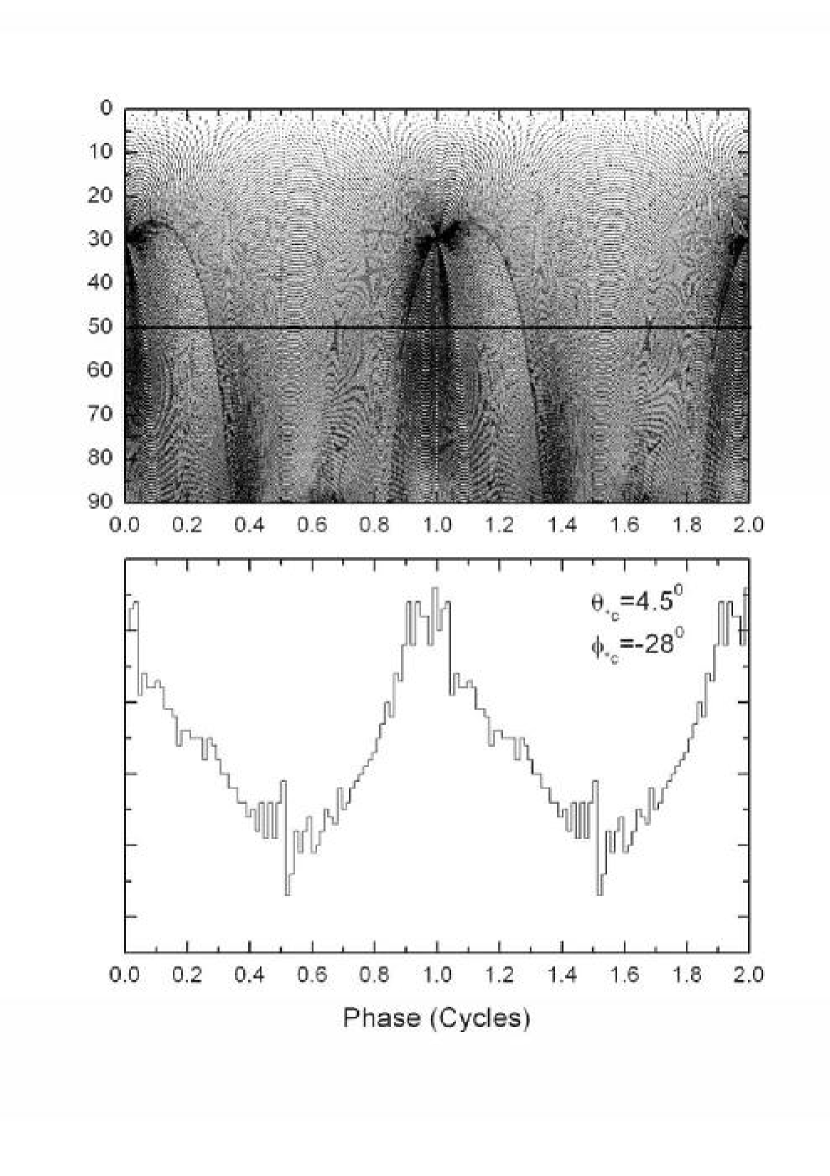
Figure 2: Upper: Emission projections on the $(\zeta,\Phi)$-plane produced by the emitting region with azimuthal width of $\Delta\phi_{\ast}=180^{0}$ at layer $a_{1}=15$. The solid line indicates the line of sight at the viewing angle $\zeta=50^{0}$, and the darker regions correspond to greater intensities. Lower: The single sinusoidal pattern of pulse profile corresponding to $\zeta=50^{0}$. SGR 1860-20 parameters are used in the calculation, and other parameters for fitting are given in Table.1.

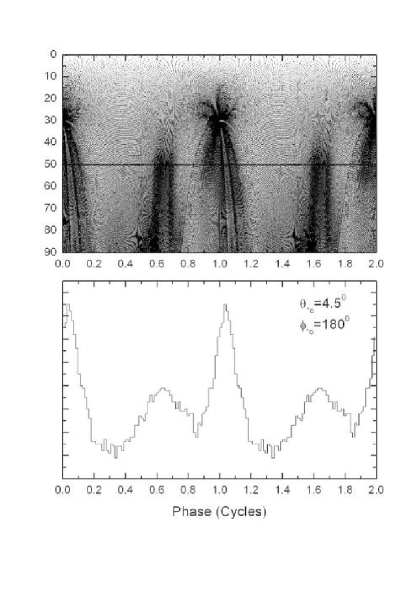
Figure 3: Upper: Emission projections on the $(\zeta,\Phi)$-plane. The same fitting parameter as those in Fig.2 except $\phi_{\ast c}$. Lower: The double-peaked pattern of pulse profile corresponding to $\zeta=50^{0}$.

Figure 4: Simulated pulsed profiles of SGR 1806-20 in the giant flare on 27 December 2004. The emitting region drifts along the azimuthal direction, with the center coordinates indicated. The arrows in panel c indicate the positions of the minor peaks of the radiation from both magnetic poles.

Figure 5: Simulated pulsed profiles of SGR 1806-20 in the giant flare on 27 December 2004. The arrows indicate the positions of the minor peaks of the radiation from both magnetic poles. The emitting region drifts in the direction perpendicular to that in Fig.4.

Figure 6: Variation of radial distance of the local position where the arrival photons are generated with the pulse phase in Fig.4.

Figure 7: The speed of the emitting region drift in $\phi_{\ast}$ direction is calculated by the comparison between our numerical results in Fig.4 and the observation. The speed is given by $v_{\phi_{\ast}}(t=\frac{t_{1}+t_{2}}{2})=\Delta x/\Delta t$, where $\Delta x$ is the displacement of the emitting region centers in two adjacent panels in Fig.4, and $\Delta t=t_{2}-t_{1}$ is the time interval. $\Delta t$ and error of $t$ is roughly determined from the time scale of Supplementary Figure 1 in Palmer et al. (2005). The error of $v_{\phi_{\ast}}$ is calculated from the error propagation $\sigma(v_{\phi_{\ast}})/\bar{v}_{\phi_{\ast}}=\sigma(t)/\bar{t}$. Since the emitting region changes the direction of movement or stops moving after $t=160~{}\rm{s}$, we set $v_{\phi_{\ast}}(t=160~{}\rm{s})\approx 0$.

Table 1: Parameter sets in Fig.2-5.

plot label	typical layer $a_{1}$	$\theta_{\ast c}(^{0})$	$\phi_{\ast c}(^{0})$	$\Delta\Phi_{\ast}(^{0})$
Fig.2	15	4.5	-28	$180$
Fig.3	15	4.5	180	$180$
panel a in Fig.4	10	3.0	-11	$180$
panel b in Fig.4	10	3.0	0	$180$
panel c in Fig.4	10	3.0	7.5	$180$
panel d in Fig.5	20	6.0	7.5	$180$

Note. — $(\theta_{\ast c},~{}\phi_{\ast c})$ are the magnetic coordinates of the middle point of the emitting region, where $\theta_{\ast c}=a_{1}\times\theta_{p}$ is the product of the layer parameter and the angular radius of the polar cap, and $\phi_{\ast c}=0^{0}$ is defined as the $\Omega$-$\mu$ plane. $\Delta\phi_{\ast}$ is the transverse extension of the emitting region along the azimuthal direction. The magnetic inclination angle is $\alpha=30^{0}$, and the viewing angel is $50^{0}$.

References

- Arendt & Eilek (1998) Arendt, P. N., & Eilek, J. A. 1998, astro-ph/9801257
- Chau, Cheng & Ding (1992) Chau, H. F., Cheng, K. S., & Ding, K. Y. 1992, ApJ, 399, 213
- Cheng, Ho & Ruderman (1986) Cheng, K. S., Ho, C., & Ruderman, M. A. 1986, ApJ, 300, 500
- Cheng, Ruderman & Zhang (2000) Cheng, K. S., Ruderman, M. A. & Zhang, L. 2000, ApJ, 537, 964
- Chiang & Romani (1994) Chiang, J., & Romani, R. W. 1994, ApJ, 436, 754
- Daugherty & Harding (1996) Daugherty, J. K., & Harding, A. K. 1996, ApJ, 458, 278
- Ding, Cheng & Chau (1993) Ding, K. Y., Cheng, K. S., & Chau, H. F. 1993, ApJ, 408, 167
- Dyks & Rudak (2003) Dyks, J., & Rudak, B. 2003, ApJ, 598, 1201
- Fernández & Thompson (2007) Fernández, R., & Thompson, C. 2007, ApJ, 660, 615
- Feroci et al. (2001) Feroci, M., Hurley, K., Duncan, R. C. & Thompson, C. 2001, ApJ, 549, 1021
- Goldreich & Julian (1969) Goldreich, P., & Julian, W. H. 1969, ApJ, 157, 869
- Harding (1981) Harding, A. K. 1981, ApJ, 245, 267
- Hurley et al. (1999) Hurley, K., et al. 1999, Nature, 397, 41
- Hurley et al. (2005) Hurley, K., et al. 2005, Nature, 434, 1098
- Jia et al. (2007) Jia, J. J., Tang, A. P. S., Takata, J., Chang, H. K., & Cheng, K. S. 2007, J. Adv. Space Res., in press
- Mazets et al. (1979) Mazets, E. P., et al. 1979, Nature, 282, 587
- Palmer et al. (2005) Palmer, D. M., et al. 2005, Nature, 434, 1107
- Romani & Yadigaroglu (1995) Romani, R. W., & Yadigaroglu, I.-A. 1995, ApJ, 438, 314
- Ruderman (1991) Ruderman, M. 1991, ApJ, 382, 587
- Ruderman & Sutherland (1975) Ruderman, M., & Sutherland, P. A. 1975, ApJ, 196, 51
- Ruderman, Zhu & Chen (1998) Ruderman, M., Zhu, T. H., & Chen, K. Y. 1998, ApJ, 492, 267
- Thompson & Duncan (1995) Thompson, C., & Duncan, R. C. 1995, MNRAS, 275, 255
- Thompson & Duncan (1996) Thompson, C., & Duncan, R. C. 1996, ApJ, 473, 322
- Thompson, Lyutikov & Kulkarni (2002) Thompson, C., Lyutikov, M., & Kulkarni, S. R. 2002, ApJ, 574, 332
- Woods et al. (2007) Woods, P. M., et al. 2007, ApJ, 654, 470
- Woods & Thompson (2004) Woods, P. M., & Thompson, C. 2004, astro-ph/0406133
- Yadigaroglu (1997) Yadigaroglu, I.-A. 1997, Ph.D. thesis, Stanford Univ.