Taking a shower in Youth Hostels: risks and delights of heterogeneity

Abstract

Tuning one’s shower in some hotels may turn into a challenging coordination game with imperfect information. The temperature sensitivity increases with the number of agents, making the problem possibly unlearnable. Because there is in practice a finite number of possible tap positions, identical agents are unlikely to reach even approximately their favorite water temperature. We show that a population of agents with homogeneous strategies is evolutionary unstable, which gives insights into the emergence of heterogeneity, the latter being tempting but risky.

I Introduction

Taking a shower can turn into a painful tuning and retuning game when many people take a shower at the same time if the flux of hot water is insufficient. In this fascinating game, it is in the interest of everybody not only to reach an agreeable equilibrium temperature but also to avoid large fluctuations. These two goals are difficult to achieve because one inevitably not only has incomplete information about the behavior and personal preferences of the other bathers, but also about the non-linear intricacies of the plumbing system.

The central issue of this paper is to find the conditions under which the agents are satisfied, which depends on the learning procedure and on its parameters.

The need to depart from rational representative agents was forcefully voiced among others by Kirman kirman_06 and Arthur and Brian Arthur, for instance in his El Farol bar problem Arthur , subsequently simplified as Minority Game CZ97 ; MGbook , from which we shall borrow some ideas concerning the learning mechanism. In these models, the agents try to behave maximally differently from each other, hence the need for heterogeneous agents.

The Shower Temperature Problem is different in that the perfect equilibrium is obtained when all the agents behave exactly in the same optimal, unique way. A priori, it is a perfect example of a case where the representative agent approach applies fully. As we shall see, however, because in practice there is a maximum number of tap tuning settings, it may pay off to be heterogeneous with respect to the strategy sets. Therefore, the problem we propose in this paper is another example of a situation where heterogeneity is tempting because potentially beneficial. The intrinsic and strong non-linearity of the temperature response function prevents the use of the mathematical machinery for heterogeneous systems that successfully solved the Minority Game MGbook ; CoolenBook , the El Farol bar problem CMO03 and the Clubbing problem TobiasClubbing .

II The Shower Temperature Problem

One of the problems of poor plumbing systems is the interaction between the water temperatures of all the people taking a shower simultaneously. If one person changes her shower setting, she influences the temperature of all the other bathers. Cascading shower tuning and retuning may follow. A key issue is how people can learn from past temperature fluctuations how to tune their own shower so as to obtain an average agreeable temperature $\hat{T}$, and also to avoid large temperature fluctuations.

Some rudimentary shower systems allow only for one degree of freedom, the desired fraction of hot water in one’s shower water, denoted by $\phi\in[0,1]$. Assuming that $H$ and $C$ denote the maximal fluxes of hot and cold water available to a shower, and that the total flux at this shower is constant, the obtained temperature is equal to

$$T=\frac{\phi HT_{H}+CT_{C}(1-\phi)}{\phi H+C(1-\phi)},$$ (1)

where $T_{H}$ and $T_{C}$ denote the constant temperatures of hot and cold water.

In the following, we shall consider the special case were $H=C$, $T_{C}=0$, and $T_{H}=1$, which amounts to express $T$ in $T_{H}$ units, i.e., to rescale $T$ by $T_{H}$, which leads to $T=\phi$.

The situation may become more complex however if many people take a shower at the same time. Indeed, it sometimes happens that altogether the $N$ bathers ask for a larger hot water flux than the plumbing system can provide, a feature more likely found in old-style youth hostels than in more upmarket hotels (hence the title). Assume that the total available hot water flux for all bathers together is $H$ while the cold water flux available at each single shower is $C=H$. We denote by $\Phi=\sum_{i=1}^{N}\phi_{i}$ the total fraction of asked hot water. If $\Phi>1$, each agent will only receive $\phi_{i}/\Phi$ instead of $\phi_{i}$ and the total flux of hot water she obtains is smaller than expected. Finally, agent $i$ obtains

$$T_{i}=\frac{\phi_{i}}{\phi_{i}+\Psi(1-\phi_{i})},$$ (2)

where $\Psi=\max(1,\Phi)$. Clearly, $T_{i}(\phi_{i}=0)=0$ and $T_{i}(\phi_{i}=1)=1$. When $\Phi\leq 1$, this equation reduces to the no-interaction case $T_{i}=\phi_{i}$. Therefore, provided that $\Phi>1$, the agents interact through the temperature they each obtain, that is, via $\Phi$. Assuming no inter-agent communication, the global quantity $\Phi$ is the only means of interaction. Therefore, this model is of mean-field nature. Henceforth, we consider the more involved case of interaction, i.e., $\Phi>1$.

III Tuning one’s shower

III.1 Equilibrium and sensitivity: the homogeneous case

Before setting up the full adaptive agent model, we shall discuss the homogeneous case where $\phi_{i}=\phi$.

Assuming that all the agents have the same favorite temperature ($\hat{T}_{i}=\hat{T}\leq 1$), they do not interact if $N\leq 1/\hat{T}$, in which case $\phi=\hat{T}$. If $N>1/\hat{T}$ the equilibrium is reached when

$$\phi=\phi_{\rm eq}=1-\frac{1}{N}\left(\frac{1}{\hat{T}}-1\right).$$ (3)

Hence, there is always a $\phi$ that satisfies everybody (for instance, setting $\hat{T}=1/2$ leads to $\phi_{\rm eq}=1-1/N$). In equilibrium each agent actually gets $\phi_{eq}H/(N\cdot\phi_{eq})=C/N$ hot water instead of $\phi_{eq}H$ and thus a total water flux of $C/N+(1-\phi_{eq})C=C/(N\hat{T})$. Hence, indeed the desired temperature $\hat{T}$ is reached for every agent, but the total water flux per agent is quite small for large $N$.

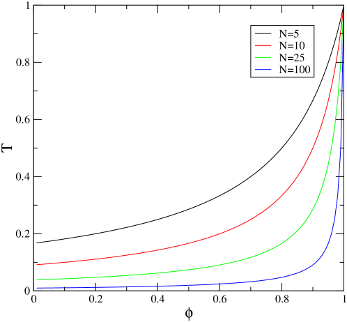
Figure 1: Individual temperature as a function of $\phi$ in the homogeneous case for increasing $N$ (from top to bottom).

The sensitivity of $T$ to $\phi$, defined as $\chi=\frac{\textrm{d}T}{\textrm{d}\phi}=\frac{N}{[1+N(1-\phi)]^{2}}$ is an increasing function of $\phi$ and maximal at $\phi=1$ (a similar result also holds for $T_{i}=\frac{\phi_{i}}{\phi_{i}+\Phi(1-\phi_{i})}$). The problem is that $\chi(\phi_{\rm eq})=N\hat{T}^{2}\propto N$; therefore, as $N$ increases, tuning $\phi$ around $\phi_{\rm eq}$ becomes more and more difficult, suggesting already that the agents might experience difficulties to learn how to tune their shower. Figure 1 illustrates this phenomenon: as $N$ increases, the region in which most of the variation of $T$ occurs shrinks substantially.

This problem is made worse by the fact that, in practice, there is only a finite number $S_{\rm max}$ of $\phi$s that can be effectively used by the agents, mostly because of internal tap static friction—the larger the friction, the smaller the number of different achievable $\phi$s. Assuming that the resolution in $\phi$ is $\delta\phi$, or equivalently that $S=1/(\delta\phi)$ values of $\phi$ are usable, it becomes impossible to tune one’s shower if $|T(\phi_{\rm eq}\pm\delta\phi)-\hat{T}|\simeq\chi(\phi_{\rm eq})\delta\phi$ is larger than some acceptable value. As $\chi\propto N$ around $\phi_{\rm eq}$, $S\propto N$ is needed; as a consequence, the ideal temperature is not learnable beyond a number of agents, which is for a large part pre-determined by the plumbing system.

III.2 Learning

The question is how to reach $\phi_{\rm eq}$. In this model, it is hoped that the agents have a common interest to avoid large fluctuations of $T_{i}$ around their favorite temperature $\hat{T}_{i}$: the Shower Temperature Problem is a repeated coordination game (cf. crawford_haller_90 and bhaskar_00 ) with many agents and limited information.

The dynamics of the agents are fully determined by their possible tap settings, thereafter called strategies, and by the trust they have in them. Each agent $i$ has $S$ possible strategies $\phi_{i,s}$ with $s=1,...,S$ chosen in $[0,1]$ before the game begins and kept constant afterwards (how to choose the $\phi$s is discussed in the next section). The typical resolution in $\phi$ is $1/S$; for the same reason, the typical maximal $\phi_{i}$ over all the agents is of order $1-1/S$. This paper follows the road of inductive behavior advocated by Brian Arthur: to each possible choice $\phi_{i,s}$ agent $i$ attributes a score $U_{i,s}(t)$ (where $t$ denotes the time step of the game), which describes its cumulated payoff at time $t$. The agents choose probabilistically their $\phi_{i,s}$ according to a logit model $P(\phi_{i}(t)=\phi_{i,s})=\exp(\Gamma U_{i,s}(t))/Z$, where $Z$ is a normalization factor and $\Gamma$ is the rate of reaction to a relative change of $U_{i,s}$.

If one were to follow blindly El Farol bar problem and Minority Game literature, one would write

$$U_{i,s}(t+1)=U_{i,s}(t)+\phi_{i,s}\left[\hat{T}_{i}-T_{i}(t)\right].$$

When $S>2$, such payoffs are not suitable any more, as the agents switch between their highest and smallest $\phi_{i,s}$, the intermediate ones being sometimes used only because of fluctuations induced by the stochastic strategy choice. A payoff allowing for a gradual increase of $\phi_{i,s}$ is necessary. Absolute value-based payoffs are fit for this purpose: mathematically,

$$U_{i,s}(t+1)=U_{i,s}(t)-\left|\hat{T}_{i}-T_{i}(t)\right|.$$

This payoff however does not depend on $\phi_{i,s}$. As a consequence, all the strategies have the same payoff. Therefore, one has to give more information to the agents. An agent that has perfect information about the plumbing system, the temperatures and fluxes of hot and cold water — for instance the plumber that built the whole installation — may know precisely which temperature she would have obtained, had she played $\phi_{i,s^{\prime}}$ instead of her chosen action $\phi_{i,s_{i}(t)}$. Such people are probably not very frequent amongst the general population, however. This is why we shall consider an in-between case, where the agents’ estimation of $T_{i,s}(t)$ is a linear interpolation between the temperature of the strategy currently in use, i. e. $T_{i}(t)=T_{i,s_{i}(t)}$ and its correct virtual value. The payoff is therefore

$$U_{i,s}(t+1)=U_{i,s}(t)(1-\lambda)-\lambda\left|\hat{T}_{i}-(1-\eta)T_{i}(t)-\eta T_{i,s}(t)\right|,$$ (4)

where $\eta\in[0,1]$ encodes the ability of the agents to infer the influence of $\phi_{i,s}$ on the real temperature and $0\leq\lambda<1$ introduces an exponential decay of cumulated payoffs, with typical score memory length $\propto 1/\lambda$. The parameter $\eta$ is related to the difference between naive and sophisticated agents as defined by Rustichini rustichini . The first kind of agents believe that they are faced with an external process, i. e. that they do not contribute to $\Phi$, whereas sophisticated agents are able to compute $\Phi_{-i}=\Phi-\phi_{i}$. In this model, perfect sophisticated agents have $\eta=1$.

IV Results

It is natural to measure two collective quantities, the average temperature $T$ obtained by the agents and its average distance from ideal temperature averaged over all the agents, denoted by ${\Delta T}=T-\hat{T}$; this characterizes the average temperature obtained by the agents, or how far the agents are collectively from their goal. The individual dissatisfaction is the distance from the ideal temperature for a given agent; one therefore measures it with ${|\delta T|}=\frac{1}{N}\sum_{i=1}^{N}|T_{i}-\hat{T}_{i}|$; it is a measure of the average risk.

All the quantities reported here are measured in the stationary state over $10,000$ time steps for $\hat{T}=0.5$, $\eta=1$, $\lambda=0.001$ and if not stated differently $N=20$, after an equilibration time of $30/(\lambda\Gamma)$. The stationary state does not depend much on $\lambda$. On the other hand, the performance of the population is of course improved as $\eta$ increases and saturates for $\eta>0.5$. The role of $\Gamma$ is discussed below.

IV.1 Homogeneous population

Since the equilibrium is reached when all the agents tune their shower in exactly the same way, trying first homogenous agents (or equivalently a representative agent) makes sense a priori. We shall therefore set $\phi_{i,s}=\phi_{s}=\frac{s}{S+1}$, $s=1,...,S$ so that the agents avoid using only hot or cold water.

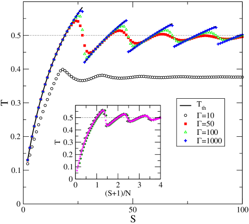
Figure 2: Temperature $T$ reached by homogeneous agents as a function of $S$ for various $\Gamma$. Inset: $T$ vs. $(S+1)/N$, showing the scaling property of $T$, with $N=10,20,40$ (asterisks, triangles, crosses).

Agents with homogeneous strategies have a peculiar way of converging to their ideal temperature as $S$ increases. Figure 2 displays the oscillations of the reached temperature with decreasing amplitude as a function of $S$. The asymmetric upward and downward slopes are due to the asymmetry of $T$ around $\phi_{\rm eq}$, as seen in Fig. 1. Theoretically, this can easily be explained by assuming that all the agents select the same $s$ that gives $T$ as close as possible to $\hat{T}$. If $s$ was a real number, $\hat{s}=[1-1/N(1/\hat{T}-1)](S+1)$. The choice of the agents therefore is limited to $[\hat{s}]$ and $[\hat{s}]+1$ where $[x]$ is the integer part of $x$ (one may need to enforce $[\hat{s}]<S$ when $S<N$). $T([\hat{s}])$ and $T([\hat{s}]+1)$ are alternatively closest to $\hat{T}$, therefore this actual optimal temperature $T_{\rm th}$ (whichever $T([\hat{s}])$ or $T([\hat{s}]+1)$) oscillates around $\hat{T}$, as seen in Fig. 2. The period of the oscillations is $N$, and their amplitude decreases as $1/S$. As expected, a very large value of $\Gamma$ replicates closely the dented nature of the value of $T_{\rm th}$, in which case all the agents take the same choice even close to the peak of $T_{\rm th}$. Generally, smaller $\Gamma$s (at least to a certain degree) lead to better average temperatures as it allows to play mixed strategies, and thus combine two temperature so as to achieve a collective average result closest to $\hat{T}$. From that point of view, $\Gamma=50$ is a better choice than $\Gamma=1000$. Hence, there exists an optimal global value of $\Gamma$, leading to a mixed-strategy equilibrium. This is because taking stochastic decisions is a way to overcome the rigid structure imposed on the strategy space, whose inadequacy is reinforced by the strong non-linearity of $T(\phi)$. Too small a $\Gamma$ is detrimental as it allows for using $\phi$ further away from $\phi_{\rm eq}$; because of the shape of $T(\phi)$, those with smaller $\phi$ are more likely to be selected.

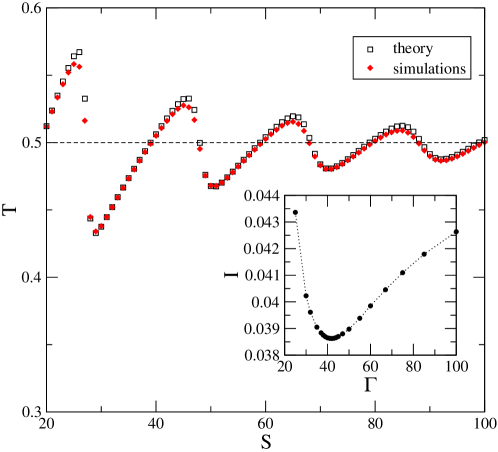
Figure 3: Temperature $T$ reached by homogeneous agents as a function of $S$ for $\Gamma=100$. Squares: theory, circles: numerical simulations. Inset: average deviation $I$ from $\hat{T}$ versus $\Gamma$ (same parameters); the dotted lines are for eye guidance only.

The individual dissatisfaction $|\delta T|$ unsurprisingly mirrors $|\Delta T|$ since all the players are identical. Both quantities are the same for large $\Gamma$ as everybody plays the same fixed strategy. $|\delta T|$ also decreases as $1/S$ (see Fig. 5). However, the larger $\Gamma$, the smaller $|\delta T|$, as each agent manages to get closer to the optimal choice.

It is easy to obtain analytical insights by solving the stationary state equations for $U_{i,s}$ (4). For the sake of simplicity, assuming that $\eta=1$ and that only the two $\phi$s surrounding $\phi_{\rm eq}$, i. e. $[\hat{s}]$ and $[\hat{s}]+1$, denoted by $-$ and $+$ respectively, are used, one obtains the set of equations (independent from $\lambda$ and $i$)

$$U_{i,\pm}=U_{\pm}=-|T_{\pm}-\hat{T}|$$ (5)

where

$$T_{i,\pm}=T_{\pm}=\frac{1}{1+\frac{N_{+}\phi_{+}+N_{-}\phi_{-}}{\phi_{\pm}}(1-\phi_{\pm})}$$ (6)

with $N_{\pm}=N\cdot P(s=\pm)$, where $P(s=+)=\frac{\exp(\Gamma U_{i,+})}{\exp(\Gamma U_{i,+})+\exp(\Gamma U_{i,-})}$ and $P(s=-)=1-P(s=+)$ is a Logit model for the two-strategy case $S=2$. Figure 3 shows the good agreement between numerical simulations and this simple theory, especially in the convex part of the oscillations, as long as $\Gamma$ is large enough to prevent the use of more than 2 strategies.

Being faced with oscillations (as a function of $S$ or $N$) of the expected value of $T$ is problematic for homogeneous agents since they do not know $N$ a priori and because $N$ may vary with time, leading to dramatic shifts of $\hat{T}$. In addition, since all the agents select the same $\phi$ for large $\Gamma$, not a single agent is ever likely to reach a temperature close to $\hat{T}$. The agents do not know whether on average they will overheat or chill. A way to measure this uncertainty is to measure the average $|{\Delta T}|$ over $S$ in numerical simulations, for instance with $I=\sum_{S=N}^{5N}|{\Delta T}|/(4N)$. The inset of Fig 3 reports that the minimum of $I$ is at $\Gamma\simeq 42$ for the chosen parameters, which shows the existence of an optimal learning rate. Since the individual satisfaction is maximal in the limit $\Gamma\to\infty$ (see above) there is no minimum of a similar measure for $|\delta T|$.

IV.2 Heterogeneous populations

Figure 4: Absolute temperature deviation $|{\Delta T}|$ reached by homogeneous (squares) and heterogeneous (circles) agents as a function of $S$ for $\Gamma=100$. Average over 500 samples for heterogeneous agents.

There are many ways for agents to be heterogeneous. One could imagine to vary $S$, $\Gamma$, $\eta$, $\lambda$ or $\hat{T}$ amongst the agents. Here we focus on strategy heterogeneity, i. e. the agents face showers with different tap settings: the strategy space of agent $i$ is no longer $\frac{1}{S+1},\ldots,\frac{S}{S+1}$, but now each agent has an individual strategy space where each strategy $\phi_{i,s}$, $s=1,\ldots,S$, is assigned a random number from the uniform distribution on $[0,1]$ before the simulation.

Intuitively, the effect of heterogeneity is to break the structural rigidity of the strategy set of a representative agent. Figure 4 reports that $|{\Delta T}|$ does not oscillate, but converge (from below) faster than $S^{-1}$ to zero. Homogeneous agents might achieve a better average temperature depending on $N$ and $S$, but on the whole clearly perform collectively worse. This is simply because most likely homogeneous agents have a $\phi$ whose difference with $\phi_{eq}$ is smaller than $1/(S+1)$ In addition, heterogeneous agents expect to have a smaller than ideal temperature, but on average predictably smaller, with no strong dependence on $S$. Thus, the expectation over the temperature of the agents is much improved by heterogeneity.

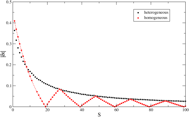
Figure 5: Individual dissatisfaction $|{\delta T}|$ reached by homogeneous (empty squares) and heterogeneous agents (full circles) as a function of $S$ for $\Gamma=1000$. Average over 500 samples for heterogeneous agents. Dashed line: theoretical predictions.

However, looking at the average absolute individual deviation from $\hat{T}$ reveals that the uncertainty brought by heterogeneity is considerably worse on average. Plotting $|\delta T|$ for both types of agents shows that $|\delta T|$ is always smaller for homogeneous agents (Fig. 5). This means that if being heterogeneous is more risky. Which agent (or equivalently, shower) performs better depends not only on $N$, but also on the tuning settings of all the agents.

IV.3 Homegeneous vs heterogeneous

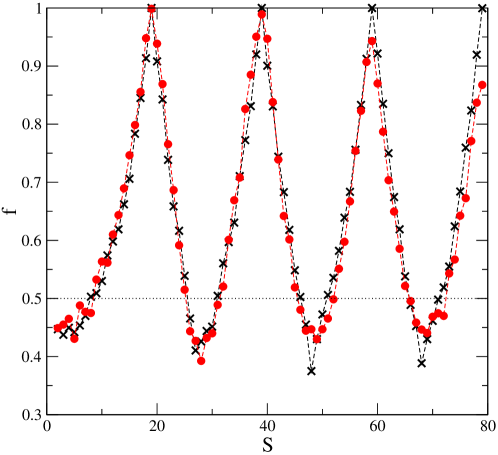
Figure 6: Fraction of the runs for which a single heterogeneous agent is worse off than the other $N-1$ homogeneous agents; $\Gamma=1000$ (crosses) and $\Gamma=30$ (circles). Average over 2000 samples.

Heterogeneity may be tempting as it suppresses the systematic abrupt oscillations experienced by homogeneous populations when $N$ changes and is collectively better on average. However, heterogeneous showers are potentially more risky. In other words, the agents must consider the trade-off between the temptation of an expected better temperature and a potentially larger deviation.

The situation discussed above is only global. Does it pay to be heterogeneous for a single agent? An answer comes from a system consisting of $N-1$ homogeneous agents as defined above and a single random one with random $\phi_{i,s}$s. The fraction $f$ of the runs at fixed $S$ that give a better $\delta T_{i}$ to the homogeneous showers is reported in Fig. 6; this quantity indicates that the majority of heterogeneous agents are not worse off for about a quarter of the values of $S$. This finding is not in contradiction with the fact that the average personal dissatisfaction of heterogeneous agents is always larger than that of homogeneous agents: $|\delta T|$ is much influenced by large deviations contributed by a minority of agents because of large temperature sensitivity to small deviations in $\phi$. Finally, the advantage of the homogeneous population increases with $\Gamma$, as a large learning rate helps only using one’s best strategy.

Let us finally give to all agents the possibility to use either strategies from the homogeneous set, or strategies drawn at random. A simple way to achieve this is to give the agents $2S$ strategies, $S$ of them defined homogeneously, and $S$ of them drawn at random before the game begins. We shall then be interested in $f_{\mathrm{h}}$, the average fraction of players using strategies from the homogeneous set. It turns out that when $\eta=1$, this fraction fluctuations as a function of $S$, for instance, but remains roughly constant. A more interesting behaviour come from varying $\eta$ (see Fig. 7). When $\eta=0$, the population is not expected to show any preference since all the score updates are the same for a given agent. Then, as $\eta$ is increased, the discrimination power of the agents improves. Quite peculiarly, a peak of advantageous homongeneity arises around $\eta\simeq 0.3$. The saturation of $f_{\mathrm{h}}\simeq 0.42$ for $\eta>0.5$ shows that in that case most agents stick to a heteregeneous strategy. Still, homogeneity and heterogeneity coexist. This probably comes from the statistical properties of distributions of random strategies around $\phi_{eq}$ together with the very strong non-linearity of $\hat{T}$ as a function of $\phi$

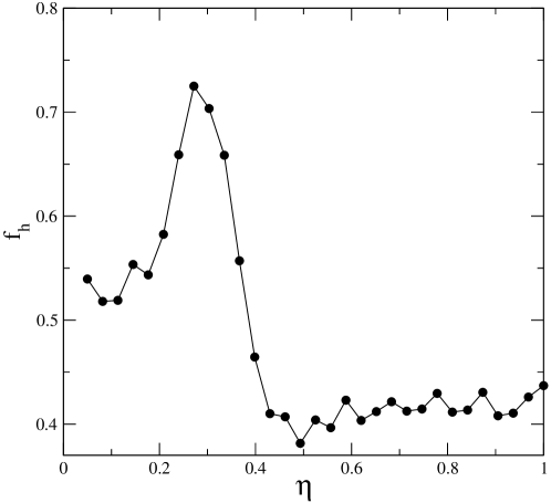
Figure 7: Fraction of the agents using one of their homogeneous strategies as a function of $\eta$; $\Gamma=100$. Average over 2000 samples.

V Discussion and conclusions

As a final note, minimizing $|\Delta T|$ is equivalent to solving a number partitioning problem GareyJohnson in which one splits a set of $N$ numbers $a_{i}>0$ into two subsets, so that the sums of the numbers in the subsets are as close as possible, which amounts to minimize $C=|\sum_{i}s_{i}a_{i}|$ where $s_{i}=\pm 1$; it is an NP-complete problem; in other words, the only way to find the absolute minimum of $C$ is to sample all the $2^{N}$ configurations. Let us consider an even simpler version of the Shower Temperature Problem that makes more explicit its NP-complete nature. Each agent $i$ is given $a_{i}$ and plays $\phi_{\rm eq}+s_{i}a_{i}$, $s_{i}=\pm 1$. Neglecting the self-impact on the resulting temperature and the non-linearity of the temperature response, the analogy between the Shower Temperature Problem and the number partitioning problem is straightforward. Methods borrowed from statistical mechanics show that the average optimal $C$ scales as $2^{-N}$, which requires to enumerate the $2^{N}$ possible configurations MertensPRL1 . This is much better than what the agents achieve; the reason for this discrepancy is that the agents do not reach a stationary state in $O(\exp N)$ time steps, hence, they cannot sample all the possible configurations. Another reason is that the optimal solution may require some agents to use a strategy that would yield a worse temperature than their optimal choice.

In conclusion, the Shower Temperature Problem shows the subtle trade-offs between a homogeneous population with equally spaced actions and a fully random one. In a system where the agents’ action space is not likely to include the optimal equilibrium choice, heterogeneity is a way to solve more robustly, with less systematic deviation on a collective level this kind of problem, at the expense of a higher risk for individual agents. In other words, if given the choice, some agents favoured by randomness will take the opportunity to improve their fate. Therefore even simple situations where a simple representative agent approach yields a unique optimal choice, it may not be reachable because of practical constraints. And thus heterogeneity emerges.

References

- (1) A. Kirman, Journal of Economic Interaction and Coordination 1, 89 (2006)
- (2) B. W. Arthur, Am. Econ. Rev. 84, 406 (1994)
- (3) D. Challet and Y.-C. Zhang, Physica A 246, 407 (1997), adap-org/9708006
- (4) D. Challet, M. Marsili, and Y.-C. Zhang, Minority Games (Oxford University Press, Oxford, 2005)
- (5) A. A. C. Coolen, The Mathematical Theory of Minority Games (Oxford University Press, Oxford, 2005)
- (6) D. Challet, G. Ottino, and M. Marsili, Physica A 332, 469 (2004), preprint cond-mat/0306445
- (7) L. De Sanctis and T. Galla, J. Stat. Mech.(2006)
- (8) The fraction of cold water in this case is still , according to the agent’s choice, since cold water is assumed to be unrestricted.
- (9) V. P. Crawford and H. Haller, Econometrica 58, 571 (1990)
- (10) V. Bhaskar, Games and Economic Behavior 32, 247 (2000)
- (11) A. Rustichini, Games and Economic Behavior 29 (1999)
- (12) Simulations show that the average temperature is in fact a function of (cf. Figure 2) (instead of a function of and ), i. e. Figure 3 would look the same if was fixed and varied. Hence we may take the average over instead of over .
- (13) M. Garey and D. Johnson, Computers and Intractability: A Guide to NP-Completeness Freeman (Freeman, New-York, 1979)
- (14) S. Mertens, Phys. Rev. Lett. 81, 4281 (1998)