Continuing dynamic assimilation of the inner region data in hydrodynamics modelling: Optimization approach

Zusammenfassung

In meteorological and oceanological studies the classical approach for finding the numerical solution of the regional model consists in formulating and solving the Cauchy-Dirichlet problem. The related boundary conditions are obtained by linear interpolation of data available on a coarse grid (global data), to the boundary of regional model. Errors, in boundary conditions, appearing owing to linear interpolation may lead to increasing errors in numerical solution during integration. The methods developed to reduce these errors deal with continuous dynamic assimilation of known global data available inside the regional domain. Essentially, this assimilation procedure performs a nudging of large-scale component of regional model solution to large-scale global data component by introducing the relaxation forcing terms into the regional model equations. As a result, the obtained solution is not a valid numerical solution of the original regional model. In this work we propose the optimization approach which is free from the above-mentioned shortcoming. The formulation of the joint problem of finding the regional model solution and data assimilation, as a PDE-constrained optimization problem, gives the possibility to obtain the exact numerical solution of the regional model. Three simple model examples (ODE Burgers equation, Rossby-Oboukhov equation, Korteweg-de Vries equation) were considered in this paper. The result of performed numerical experiments indicates that the optimization approach can significantly improve the precision of the sought numerical solution, even in the cases in which the solution of Cauchy-Dirichlet problem is very sensitive to the errors in the boundary condition.

Studying and modelling different physical processes frequently require to solve the Cauchy-Dirichlet problem. In geophysical investigations, for solving of the Cauchy-Dirichlet problem, numerical methods are usually applied. The discrete form of equations and initial and boundary values at the points of the grid are traditionally used in these methods. The problem is generally solved by using a proper numerical scheme. However, both initial and boundary values, which are obtained from measurements or other model outputs, contain errors, which can reach $30\%$ from the true values.

For some problems, the solution can be very sensitive to these errors. At the same time some values of the sought solution at some points of the inner region, along with initial and boundary data, are often available. These additional data also have errors. The question arises: Is it possible to improve the accuracy of the solution of the Cauchy-Dirichlet problem by using these additional data (which may contain errors)? For some well-known equations of mathematical physics and dynamic meteorology we will show here that the use of additional information on the solution values within the integration region can noticeably improve the accuracy of the sought solution.

An improvement of the solution accuracy of the Cauchy-Dirichlet problem is extremely important in meteorology because this is the problem of regional weather forecast. A distinction between two types of atmospheric forecast models needs to be done. These are global models, making forecast for the whole earth, and regional models, which produce a forecast for a limited region. One of basic differences between these model types is the grid resolution. Global models use a low resolution space grid and regional models operate on a more dense mesh. The reason for the existence of these two model types is, basically, computational. Even nowadays it is not possible in acceptable time period to integrate global models with the detailed physics and with the space resolution of regional models. It is worth noticing that global and regional models include different physical processes. Global models describe large-scale slow-time varying processes, with the time period of more than 3 hours and the space scale larger than 60 km. Regional models can simulate the evolution of mesometeorological fast processes (small cyclones, storms, tornados), with the time period of less than 3 hours and the spatial extent between 2 and 60 km.

These models are described mathematically by systems of nonlinear partial differential equations. To solve the system corresponding to a global model we need only the initial condition and bottom and upper boundary conditions, as the domain is the whole sphere. To get the solution of a system corresponding to a regional model we also need lateral boundary conditions. Generally, the lateral boundary conditions for a regional model are obtained from the global model. Global model data corresponding to the domain of a regional model lateral boundary are interpolated into a regional mesh and then are used for finding of the Cauchy-Dirichlet problem solution.

We should notice that the lateral boundary conditions obtained from the global model do not provide any information on the structures of the scales smaller than the size of the mesh of the global model. In fact, global models do not distinguish a local meteorological phenomenon of characteristic length scale smaller than $30$ km, because the space step is greater than this value. On the other hand, the parts of space and time spectrums of a regional model solution which correspond to large-scale structures and long-period processes are in worse accordance with observations than those of a global model. This is related to the fact that a regional model does not have the information about the phenomena that occur outside its domain and therefore cannot describe with necessary precision (because the lateral boundary data are in low resolution discrete space and time grid) the impact of these phenomena on the evolution of processes inside the integration domain.

For example, the weakly regular, low frequency oscillations of the sea surface temperature near the Peru coast, known as El Niño and La Niña events, have a large influence on the climate of Brazil. The circulation regimes over the Brazilian territory noticeably differ during these events. As a result, the precipitation rate in the South of Brazil during the La Niña periods is two times smaller than during the El Niño periods. Regional models driven, for example, by the Reanalysis data do not reproduce with confidence this distinction between the El Niño and La Niña regimes. The reason of this inconsistency is, probably, poor space and time data resolution on the regional model boundaries. Mathematically, it means that we are solving boundary value problems with significant errors on the boundaries and the solution is sensitive to these errors.

The spectral nudging technique is one of methods proposed to use additional data from the inner domain in order to reduce boundary error influence and to improve a solution of initial-boundary value problem (Waldron et all., 1996; Storch et all., 2000; Kanamaru and Kanamitsu, 2005). This method supposes incorporation of the largest internal modes of some meteorological variables from observations or from a driving model into the regional model solution. However the use of the spectral nudging technique requires inserting additional forcing terms into the evolution equations of a regional model. Hence the original model is corrupted and its new solution may not be close to the exact sought solution.

In this work we propose a method which is free from the above mentioned shortcoming. Firstly, in Section 2 we give the formulation of the Cauchy-Dirichlet problem for a regional model and the general formulation of an optimization problem, and we show how the latter (with the accessibility of some additional conditions) can be applied for finding the solution of the former. In Section 3, for some simple equations, we show how the optimization approach can be used to obtain a solution of the initial boundary value problem. The equations considered here include the ordinary differential equation of Burgers, the one-dimensional, linearized Rossby-Oboukhov partial differential equation, and the partial differential equation of Korteweg - de Vries. We also compared the sensitivity of the solutions, obtained by the traditional and the new approach with respect to the errors in the boundary conditions. In Section 4 we discuss the obtained results. Appendix A provides more detailed description of the optimization procedure.

1 Numerical solution of regional problems

1.1 The numerical forecast model

We formulate here the Cauchy-Dirichlet problem as it is formulated for the regional weather forecast. To find a unique solution for the regional model equations we need the lateral boundary condition for entire time interval on which the solution is seeking. We obtain these data from the solution of an outer model which, as a rule, is a global model. We don’t know an exact solution of the outer model (if we did, our problem already would have been solved), but we can find its approximate solution in the discrete form:

$$\begin{array}[]{l}\Delta_{t}\{\Psi\}=F_{d}\textrm{,}\\ \Psi(x,0)=Y_{global}(x)\textrm{,}\\ \Psi(x,t)\mid_{x\in B}=\Psi_{b}(x,t).\end{array}$$ (1)

Here $\Delta_{t}$ is the evolution operator of the discrete model, $\Psi$ is the vector of the prognostic functions, $F_{d}$ are discrete external forces, $Y_{global}$ is the initial condition, $B$ are upper, lower (and maybe lateral) boundaries of the global model, and $\Psi_{b}$ is the boundary condition for the global model. Let $\Psi_{sl}$ will be the solution of (1). We suppose that this solution is sufficiently close to the solution of hypothetical ideal model which exactly describes the real atmospheric processes.

The regional model is located in a closed area with boundary $S$ and its discrete representation can be written in the same manner as for the global model

$$\begin{array}[]{l}\delta_{t}\{G\}=F_{rd}\textrm{,}\\ G(x,0)=Y_{local}(x)\textrm{, }\\ G(x,t)\mid_{x\in S}=G_{s}(x,t)\textrm{,}\end{array}$$ (2)

where $\delta_{t}$ is the evolution operator of the discrete regional model, $G$ is the vector of the prognostic functions and $F_{rd}$ are discrete external forces, $Y_{local}$ is the initial condition, and $G_{s}$ is the boundary condition for the regional model.

Now, we can solve numerically the initial boundary value problem (2) using the solution $\Psi_{sl}$ of the global model (1) for getting the boundary conditions. The traditional approach to seek the solution of (2) consists in the interpolation of required data from $\Psi_{sl}$ on the regional grid for forming the initial and boundary conditions and then applying any numerical method to solve the model equations. But, as we have mentioned above, the boundary conditions contain errors which can strongly corrupt the solution.

The use of the information obtained from the solution of the global model equations $\Psi_{sl}$ on the values inside the area of the regional model integration for all available time moments can help to overcome this difficulty.

1.2 Formulation of the optimization problem

We assume that the solution of regional model (2) cannot strongly differ from global model solution $\Psi_{sl}$. Our objective is to find $G_{sl}$ on the fine (regional) mesh that satisfies the initial values and the equations of the regional model (2). The solution $G_{sl}$ also have to be as close as possible to the $\Psi_{sl}$ inside the regional model domain. We can formulate this aim as an optimization problem in the following manner

$$\begin{array}[]{rl}\textrm{Minimize }&d(G,\Psi_{sl})\\ \textrm{subject to \, (s.t.) }&\delta_{t}\{G\}-F_{rd}=0,\\ &G(x,0)-Y_{local}(x)=0.\end{array}$$ (3)

Here $d(:,:)$ is the objective function, which represents the distance between $G$ and $\Psi_{sl}$ vectors. In other words, we want to minimize the distance between the regional and the global model solutions under conditions that the regional model equations and the initial condition are satisfied. Note here that, when we talk about the solution $G$, we bear in mind the vector $G=G(x,t)$ in a grid space of ($x$,$t$) - coordinates, where $t$ corresponds to discrete time points of the regional model integration and $x$ to discrete mesh points in the regional model area.

There are different approaches to solve the optimization problem (3). For example, we can apply it to each time level, as it is done in finite-differences methods: For the given initial conditions ($t_{0}=0$), the solution is obtained at $t_{1}$. Then, considering the solution at $t_{1}$ as the initial condition, the solution is found at $t_{2}$ and so on. On the other hand, we can consider the domain of definition of the problem on the mesh including all time levels. In this case all available information from the global model for the period of integration will be taken into consideration simultaneously. We use here this approach.

2 Examples of application of the optimization method to the problems of small dimension

2.1 Burgers’ equation

We shall demonstrate an application of the optimization method to problems of small dimension. As a first example we consider the supersensitive boundary value problem for the Burgers’ equation (Bohé, 1996):

$$\begin{array}[]{l}\epsilon x^{\prime\prime}=-xx^{\prime}\textrm{,}\\ x(0)=-1\textrm{, }x(T)=1.\end{array}$$ (4)

To get the analytical solution of this equation it is enough to integrate the left and right sides of the equation (4) over $t$:

$$\epsilon x^{\prime}=-\frac{x^{2}+c}{2}.$$

Then, after rewriting the foregoing formula as

$$\epsilon\frac{dx}{x^{2}+c}=-\frac{dt}{2}$$

and integrating the left side over $x$ and the right one over $t$, we can write the Burgers’ equation solution as

$$x=\begin{cases}\frac{\displaystyle\sqrt{-c}\left(1+\exp{\frac{(t+C_{2})\sqrt{-c}}{\epsilon}}\right)}{\displaystyle 1-\exp{\frac{(t+C_{2})\sqrt{-c}}{\epsilon}}},\,\,\textrm{ for }c\leq 0\textrm{,}\\ \\ \sqrt{c}\tan\left(\frac{\displaystyle(t+C_{2})\sqrt{c}}{\displaystyle 2\epsilon}\right),\,\,\textrm{ for }c>0.\end{cases}$$

The graph of the analytical solution for equation (4) with the boundary condition $x(0)=-1$, $x(1)=1$ and $\epsilon=0.05$ is presented in Figure 1. Numerical solution of this problem applying, for example, the shooting method coincides with great accuracy with the analytical one.

[Insert figure 1 here.]

Abbildung 1: Analytical solution of the Burgers’ equation for $\epsilon=0.05$ and the boundary condition:
$x(0)=-1$, $x(1)=1$.

Let us choose several points from the analytical solution and slightly perturb them (till 5% from its real value). This procedure models the boundary and inner domain data containing errors. Using these perturbed data for the boundary points $x(0)$, $x(1)$ we solve the boundary problem (4) applying the shooting method. For the step $\Delta t=0.01$ the numerical solution is presented in Figure 2 by red line.

[Insert figure 2 here.]

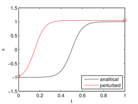
Abbildung 2: Forward problem solution with 5% perturbed boundary condition of Burgers’ equation in comparison with exact analytical solution.

As one can see, small perturbations of the boundary condition result in large errors in the solution. Now, let us solve the optimization problem (3) using additional information about the perturbed solution on the points inside the domain. Using the same discretization as when solving (4) by the traditional shooting method, with the same $\Delta t=0.01$ we find the solutions which are exhibited in Figure3.

Figure 3 shows the solutions of the optimization problem for the three cases when we used 3, 4 and 5 points of the perturbed solution, respectively. One can see that all these solutions correspond better to the analytical solution, than the solution obtained by the traditional approach. In the case of using the three additional inner points, the optimization solution and the analytical solution nearly coincide. This example shows that there are dynamical systems in which small perturbations ($\leq$ 5%) in the boundary conditions can lead to great errors in the final solution. However, if some additional information exists, it can be used to improve significantly the sought solution, applying to the considered problem the optimization theory methods.

[Insert figure 3 here.]

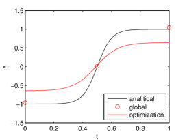
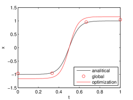
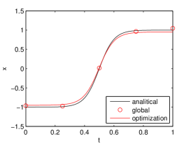
Abbildung 3: Optimization problem solution of Burgers’ equation for three cases: 3 reference points; 4 reference points; and 5 reference points.

2.2 Rossby-Oboukhov one-dimensional equation

Here we consider the one-dimensional linear partial differential equation obtained during the linearization procedure of the Rossby-Oboukhov equation (Oboukhov, 1949):

$$\frac{\partial}{\partial t}\left(\frac{\partial^{2}}{\partial x^{2}}-\frac{1}{l_{0}^{2}}\right)\psi+\beta\frac{\partial\psi}{\partial x}+U\frac{\partial^{3}\psi}{\partial x^{3}}=0\textrm{.}$$ (5)

Here $\psi$ is the stream function, $f_{0}=10^{-4}$ s^-1 is mean value of Coriolis parameter, $\beta=df/dy=1.6\cdot 10^{-11}$ s^-1m^-1 is mean value of meridional gradient of Coriolis parameter, $l_{0}=c_{0}/f_{0}=3\cdot 10^{6}$ m is the Oboukhov scale, $c_{0}$ is the sound velocity, and $U$ is the zonal wind, which is variated between $0$ and $30$ m/s.

For the periodic boundary condition

$$\psi(0,t)=\psi(L,t),$$ (6)

where $L$ is the size of integration area (we shall use $L=3\cdot 10^{7}$ m), the solution of equation (5) can be written as

$$\psi(x,t)=\sum_{n=1}^{N}A_{n}\sin[k_{n}(x-c_{n}t)+\phi_{n}]\textrm{,}$$ (7)

where

$$c_{n}=U-\frac{\beta+U/l_{0}^{2}}{k_{n}^{2}+1/l_{0}^{2}}\textrm{,}$$ (8)

$$k_{n}=\frac{2\pi n}{L},$$

and $A_{n}$ and $\phi_{n}$ are defined by the initial condition (Rossby, 1939).

For finding the numerical solution it is convenient to rewrite the equation in nondimensional form. We choose the following scales $S=6\cdot 10^{6}$ m, $T=S/V=6\cdot 10^{5}$ $s$, $V=10$ $m/s$. The dependent and independent nondimensional variables are defined as follows:

$$\tilde{x}=\frac{x}{S},\qquad\tilde{t}=\frac{t}{T},\qquad\tilde{\psi}=\frac{T}{S^{2}}\psi.$$ (9)

, and equation (5) may be written in nondimensional form as

$$\frac{\partial}{\partial\tilde{t}}\left(\frac{\partial^{2}}{\partial\tilde{x}^{2}}-\frac{1}{b^{2}}\right)\tilde{\psi}+\beta_{0}\frac{\partial\tilde{\psi}}{\partial\tilde{x}}+U_{0}\frac{\partial^{3}\tilde{\psi}}{\partial\tilde{x}^{3}}=0\textrm{,}$$ (10)

where $\frac{1}{b}=\frac{S}{l_{0}}=2$, $\beta_{0}=\frac{\beta S^{2}}{V}=57.6$ and $U_{0}=\frac{U}{V}\in[0,3]$.

For finite-difference discretization we use unconditionally stable scheme with truncation error $\mathcal{O}(\Delta x^{2},\Delta t^{2})$ given by

$$\begin{split}&\frac{1}{\Delta t}\left(\frac{\tilde{\psi}_{i+1}^{k+1}-2\tilde{\psi}_{i}^{k+1}+\tilde{\psi}_{i-1}^{k+1}}{\Delta x^{2}}-\frac{\tilde{\psi}_{i+1}^{k}-2\tilde{\psi}_{i}^{k}+\tilde{\psi}_{i-1}^{k}}{\Delta x^{2}}-\frac{1}{b^{2}}\left(\tilde{\psi}_{i}^{k+1}-\tilde{\psi}_{i}^{k}\right)\right)\\ &+\frac{\beta_{0}}{2}\left(\frac{\tilde{\psi}_{i+1}^{k+1}-\tilde{\psi}_{i-1}^{k+1}}{2\Delta x}+\frac{\tilde{\psi}_{i+1}^{k}-\tilde{\psi}_{i-1}^{k}}{2\Delta x}\right)\\ &+\frac{U_{0}}{2}\left(\frac{\tilde{\psi}_{i+2}^{k+1}-2\tilde{\psi}_{i+1}^{k+1}+2\tilde{\psi}_{i-1}^{k+1}-\tilde{\psi}_{i-2}^{k+1}}{2\Delta x^{3}}+\frac{\tilde{\psi}_{i+2}^{k}-2\tilde{\psi}_{i+1}^{k}+2\tilde{\psi}_{i-1}^{k}-\tilde{\psi}_{i-2}^{k}}{2\Delta x^{3}}\right)=0\end{split}$$

At first, we generate a specific analytical solution (7) containing 85 modes. Figure 4 shows this solution for $t=0$ h.

[Insert figure 4 here.]

Abbildung 4: Analytical solution of Rossby-Oboukhov equation on periodic domain $[0,L]$ at $t=0$ h with 85 modes.

Note that in Figures we use dimensional values, but in the numerical computations all variables are nondimensional.

As a local model we consider the equation (10), with initial and boundary conditions, defined over $[a,b]\varsubsetneq[0,L]$ (closed interval smaller than entire domain). For initial and boundary conditions we will use our specific form (see Fig. 4) of the global model solution (7). For simulating really encountered problems of atmospheric modelling we took the analytical solution in the points of the the coarse grid with space step $\Delta x=200$ km and time step $\Delta t=2$ hour, and perturb its values randomly in such a way that a perturbation can reach till 30% of its exact value.

Primarily we find the solution of the forward Cauchy-Dirichlet problem for our local model. As local domain we take the interval $[1.8\cdot 10^{7},2.4\cdot 10^{7}]m$ (6000 kilometers) inside the global model interval $[0,3\cdot 10^{7}]m$. For the first reference experiment the initial and boundary conditions were taken from the exact analytical solution (7). Requiring that the numerical solution with the exact initial and boundary condition have to nearly coincide with the analytical solution, we took as the maximal possible values of space and the time steps $\Delta x=10$ kilometers and $\Delta t=200$ seconds respectively. To obtain the solution of the forward problem described above for $96$ hours it is demanded $0.8$ second of CPU time.

[Insert figure 5 here.]

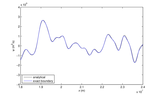
Abbildung 5: Forward problem solution with exact boundary condition of Rossby-Oboukhov equation at $96$ hours. $\Delta x=10$ km, $\Delta t=200$ sec. CPU time = 0.8 sec.

In the next experiments the perturbed analytical solution on the coarse grid was used for formation of the boundary conditions. Figure 5 shows the exact solution and the solution with perturbed boundary conditions of the forward problem.

[Insert figure 6 here.]

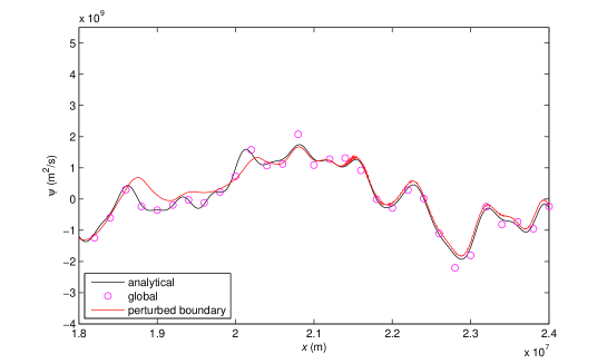
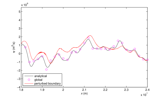
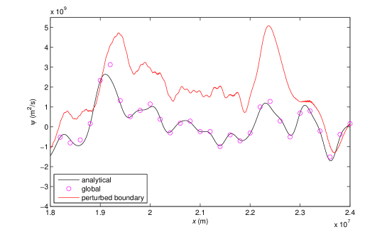
Abbildung 6: Forward problem solution with 30% perturbed boundary condition of Rossby-Oboukhov equation at $t=24$, $48$, $96$ hours. $\Delta x=10$ km, $\Delta t=200$ sec. CPU time = 0.8 sec.

One can see that for the forward problem the numerical solution rather quickly diverges from the analytical solution due to the errors of the linear interpolation procedure in the border points. After $96$ hours perturbed boundary solution has very faint resemblance with the analytical one.

In the second series of experiments we applied the optimization method to the local model. For this calculation we used all available global data (perturbed analytical solution on coarse grid) in the inner local domain. Figure 6 shows the results of calculations. It is important to note, that, as in previous experiments, we chose the space $\Delta x=100$ km and the time $\Delta t=3600$ sec steps to be as large as possible.

[Insert figure 7 here.]

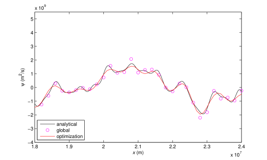
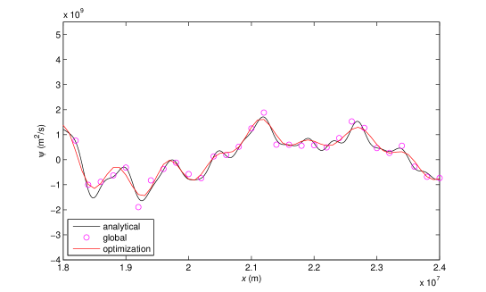
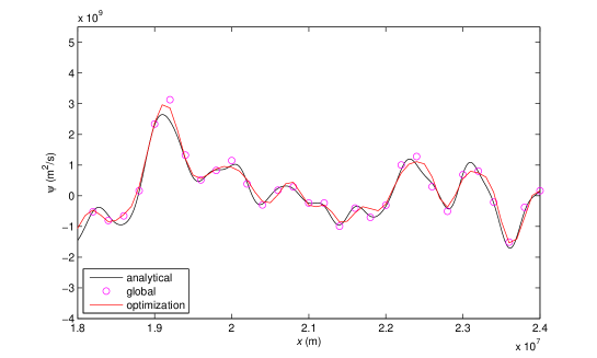
Abbildung 7: Optimization problem solution of Rossby-Oboukhov equation with 30% perturbed global solution at $t=24$, $48$, $96$ hours. $\Delta x=100$ km, $\Delta t=3600$ sec. Average CPU time = 0.5 sec.

In the optimization approach one can use larger steps than in the forward problem, because we do not deal with a time-evolution problem, and there is no accumulation of numerical errors at each time step. In Figure 7, one can see that for space and time steps many times larger than those that were used in the forward problem ($\Delta x=100$ kilometers and $\Delta t=3600$ seconds) we have far better agreement with the analytical solution. The decrease of time and/or space step in the optimization approach does not appreciably improve the solution, only the smallest details are slighly better reproduced.

As the local mesh in the optimization approach is rather coarse, the average CPU time needing for solving the problem is smoller than for forward problem ($0.5$ seconds) in spite of greater computational complexity. Also we have to pay attention on a very weak sensitivity to the global data perturbations. The impact of every individual perturbation on the optimization solution is very small. For example, increasing errors in randomly perturbed global data up to 60% does not strongly affect the solution as one can see in Figure 8.

[Insert figure 8 here.]

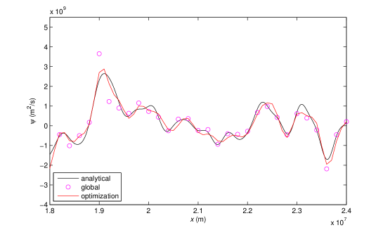
Abbildung 8: Optimization problem solution of Rossby-Oboukhov equation with 60% perturbed global solution at $96$ hours. $\Delta x=100$ km, $\Delta t=3600$ sec. Average CPU time = 0.5 sec.

These experiments clearly show that the use of additional global data inside the local domain, even perturbed, can significantly improve the solution of the model. The optimization approach, albeit seeking the solution on entire space-time grid, is not very numerically expensive, because the space, and, principally, the time steps can be chosen much larger than in the forward problem.

2.3 Korteweg-de Vries equation

Now we consider the Korteweg-de Vries equation:

$$u_{t}+6uu_{x}+u_{xxx}=0,$$ (11)

and find its numerical solution applying both the traditional forward method and the optimization method.

The equation (11) has the exact solution (Korteweg and de Vries, 1895),(Grimshaw, 2004)

$$u=b+a\,\mathrm{cn}^{2}(\gamma(x-Vt)|m),$$ (12)

where $\mathrm{cn}(x|m)$ is the Jacobi elliptic function, $m\,(0<m<1)$ is the module of elliptic function, $a=2m\gamma^{2}$ and $V=6b+4(2m-1)\gamma^{2}$. For the case when $m\to 1$ we will have $cn(x|m)\to sech(x)$ and the solution (12) will have the form

$$u=b+a\,\mathrm{sech}^{2}(\gamma(x-Vt)),$$ (13)

with $V=6b+2a$,and $a=2\gamma^{2}$ which describes a one-dimensional soliton .

For the finite-difference discretization we use the following implicit numerical scheme (Furihata, 1999), which possesses the properties of total energy and mass conservation:

$$\begin{split}&\frac{u_{i}^{j+1}-u_{i}^{j}}{\Delta t}+\frac{1}{2\Delta x}\left((u_{i+1}^{j+1})^{2}-(u_{i-1}^{j+1})^{2}+u_{i+1}^{j+1}u_{i+1}^{j}-\right.\\ &\left.-u_{i-1}^{j+1}u_{i-1}^{j}+(u_{i+1}^{j})^{2}-(u_{i-1}^{j})^{2}\right)+\frac{1}{2\Delta x^{3}}\left(\frac{u_{i+2}^{j+1}+u_{i+2}^{j}}{2}-\right.\\ &\left.-(u_{i+1}^{j+1}+u_{i+1}^{j})+(u_{i-1}^{j+1}+u_{i-1}^{j})-\frac{u_{i-2}^{j+1}+u_{i-2}^{j}}{2}\right)=0.\end{split}$$

As a numerical scheme is non-linear for obtaining of numerical solution of a forward problem we use the Newton method.

Following the steps of previos example, we choose as a reference model the analitical solution with cofficient $b=a$, $\gamma=2$ and module of elliptic function $m=0.995$. The Figure 9 represents the solution on domain $[-5,15]$ at time $t=0$.

[Insert figure 9 here.]

Abbildung 9: Analytical solution of KdV equation as the cnoidal wave (12) on the domain $[-5,15]$ at $t=0$ with $\gamma=2$, $b=a$ and module $m=0.995$.

As a local model we consider the equation (11) defined over closed interval $[0,10]$. To get a good accordance between a numerical solution of forward problem (with exact initial and boundary conditions) and an anlytical solution on the time interval $0\leq t\leq 1$ we took as the maximum possible values of space and the time steps $\Delta x=0.02$ and $\Delta t=0.0002$ respectively. The CPU time required to find the solution is 15 seconds.

[Insert figure 10 here.]

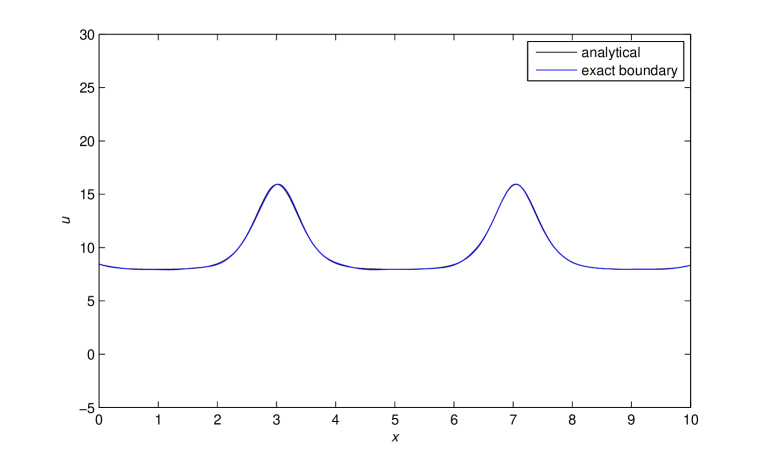
Abbildung 10: Forward problem solution with exact boundary condition of KdV equation at $t=1$. $\Delta x=0.02$, $\Delta t=0.0002$. CPU time = 15 sec.

As a global model solution we take the analytical solution, intoduced above as the reference model, with space step $\Delta x=0.5$ and time step $\Delta t=0.005$ and perturb its values till $10\%$ from the exact ones. Using these perturbed global model solution to form boundary condition for local model we will solve initially the forward problem.

[Insert figure 11 here.]

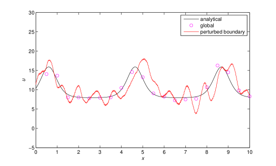
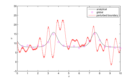
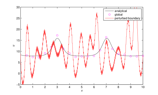
Abbildung 11: Forward problem solution with 10% perturbed boundary condition of KdV equation at time $t=0.2$, $0.5$, $1$. $\Delta x=0.02$, $\Delta t=0.0002$. CPU time = 23 sec.

In Figure 11 one can see that the forward problem with small errors in the boundary conditions can produce inacceptable numerical solution.

Now, we apply the optimization method to the local model using additional avaliable for inner points information from global model solution. Figure 12 shows the solution of the optimization problem. As in previous experiment we chose the space ($\Delta x=0.2$) and the time ($\Delta t=0.002$) steps as large as possible.

[Insert figure 12 here.]

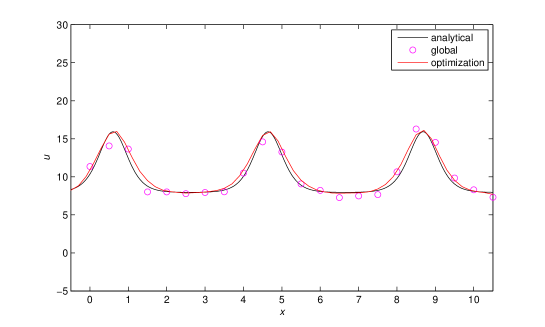
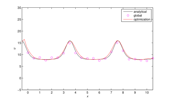
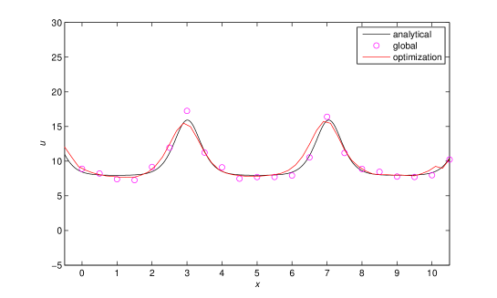
Abbildung 12: Optimization problem solution of KdV equation with 10% perturbed global solution at time $t=0.2$, $0.5$, $1$. $\Delta x=0.2$, $\Delta t=0.002$. Average CPU time = 21 sec.

It can be clearly seen the advantage of the optimization approach in this case. The difference between numerical and exact solution is very small in comparison with the forward problem calculations.

3 Discussions and conclusions

The results of the numerical experiments presented here indicate that the optimization approach can significantly improve the precision of the sought numerical solution of the regional model when the boundary values have errors but the information on the behaviour of the sought solution in a number of inner points is available. Even in the cases in which the solution of Cauchy-Dirichlet problem is very sensitive to the errors in the boundary condition the use of optimization approach gives the possibility to construct the solution which are close to the analytical solution. We also made experiments with two-dimentional nonlinear Rossby-Oboukhov equations. The preliminary results also demonstrate that the use of the optimization approach significantly improve the numerical solution of boundary problem with errors in the boundary values. At the present time we are developing economic algorithm that can be applied to any great computational problem.

Anhang A

Formulation of optimization problem

We can express our problem as the following non-linear optimization problem with equality constraints

$$\begin{array}[]{rl}\textrm{Minimize}&\frac{1}{2}\|u-V\|^{2}\\ \textrm{s.t. }&h(u)=0\textrm{,}\end{array}$$ (14)

where $V$ represents the global data on the regional mesh and $h(u)=[h_{1}(u)\,h_{2}(u)\,\ldots\,h_{m}(u)]^{T}$ is a vector of the discretizations of regional equations at each point of space-time mesh of the regional model.

A usual optimization technique to solve this kind of problem is to apply Newton’s iteration method to the system of nonlinear equations arising from first-order necessary conditions, known as Karush-Kuhn-Tucker (KKT) conditions (Nocedal and Wright, 1999). For instance, the KKT conditions for the problem (14) are

$$\begin{array}[]{rl}(u-V)+h^{\prime}(u)^{T}\lambda&=0\\ h(u)&=0\textrm{,}\end{array}$$ (15)

where

$$h^{\prime}(u)=\left(\begin{array}[]{c}\nabla h_{1}(u)^{T}\\ \nabla h_{2}(u)^{T}\\ \vdots\\ \nabla h_{m}(u)^{T}\end{array}\right)$$

is the Jacobian matrix of the constraint function and $\lambda$ represent the vector of Lagrange coefficients. Each step of the Newton iteration associated with system (15) is defined as follows:

$$\begin{array}[]{c}J(u_{k},\lambda_{k})\left(\begin{array}[]{c}\Delta u_{k}\\ \Delta\lambda_{k}\end{array}\right)=-\left(\begin{array}[]{l}u_{k}-V+h^{\prime}(u_{k})^{T}\lambda_{k}\\ h(u_{k})\end{array}\right)\\ \\ \left(\begin{array}[]{c}u_{k+1}\\ \lambda_{k+1}\end{array}\right)=\left(\begin{array}[]{c}u_{k}\\ \lambda_{k}\end{array}\right)+\left(\begin{array}[]{c}\Delta u_{k}\\ \Delta\lambda_{k}\end{array}\right)\end{array}$$ (16)

where $J$ represents the Jacobian matrix of the system (15)

$$J(u,\lambda)=\left(\begin{array}[]{ccc}I+\sum_{i}\lambda_{i}\nabla^{2}h_{i}(u)&&h^{\prime}(u)^{T}\\ \\ h^{\prime}(u)&&0\end{array}\right)\textrm{,}$$ (17)

and $\nabla^{2}h_{i}(u)$, $i=1,\ldots,m$, are Hessian matrices of the constraints.

The Jacobian matrix (17) is a saddle point matrix and there are many methods that can be applied with assosiated linear system (Benzi, Golub and Liesen, 2005). But first, note that the derivative of the discretization vector of the constraints is described by a sparse matrix with block-diagonal structure, because this derivative is calculated at every point of time-space mesh. On the other hand, the first part $I+\sum_{i}\lambda_{i}\nabla^{2}h_{i}(u)$ of Jacobian matrix (17) of the system (15) includes the calculation of the Hessians of the constraints discretization vector, which is a computationally expensive procedure because calculations have to be made for every Newton iteration. The resulting matrix is generally dense. To accelerate the calculations and reduce the consuming of the computer memory we use the following Jacobian approximation:

$$B_{k}=\left(\begin{array}[]{cc}I&h^{\prime}(u_{k})^{T}\\ h^{\prime}(u_{k})&0\end{array}\right).$$ (18)

The use of the approximation $B_{k}$ for $J(u_{k},\lambda_{k})$ strongly simplifies the procedure of finding the solution of the linear system (16) (Benzi, Golub and Liesen, 2005).