Weak measurement: Effect of the detector dynamics

Abstract

The contribution of the detector dynamics to the weak measurement is analysed. According to the usual theory [Y. Aharonov, D. Z. Albert, and L. Vaidman, Phys. Rev. Lett. 60, 1351 (1988)] the outcome of a weak measurement with preselection and postselection can be expressed as the real part of a complex number: the weak value. By accounting for the Hamiltonian evolution of the detector, here we find that there is a contribution proportional to the imaginary part of the weak value to the outcome of the weak measurement. This is due to the coherence of the probe being essential for the concept of complex weak value to be meaningful. As a particular example, we consider the measurement of a spin component and find that the contribution of the imaginary part of the weak value is sizeable.

I Introduction

The concept of weak value was introduced in AAV . It is the complex number $A_{w}=\langle S_{f}|\hat{A}|S_{i}\rangle/\langle S_{f}|S_{i}\rangle$ in terms of which one can express $\langle A\rangle$, the average result of a measurement of an observable $\hat{A}$ preceded by a preparation in the state $|S_{i}\rangle$ and followed by a postselection of the state $|S_{f}\rangle$, provided that the interaction between the system and the detector, which we shall call the probe as a reminder of its quantum nature, is weak enough compared to the coherence scale of the latter Duck .

Under the assumptions of AAV , for a weak analogue of an ideal von Neumann measurement, the average value is given by $\langle A\rangle={Re}(A_{w})$. A surprising result is that this average value can lie well outside the range of the eigenvalues of $\hat{A}$. This fact has been confirmed experimentally Ritchie ; Parks ; Pryde in optics. Also, the formalism of the weak value was proved to describe some relevant phenomena in telecom fibers Brunner2003 , and to be connected with the response function of a system Solli2004 . The possibility of performing a weak measurement in solid state systems is currently being investigated Romito . In Ref. AAV the initial state of the probe is assumed a pure gaussian state, with a special choice of the phase, and the free evolution of the probe is neglected. Since the coherence of the probe is an essential requisite for the weak value to be significant, and since the Hamiltonian evolution induces a relative phase between different components of the state of the probe, the latter assumption seems unrealistic, especially for a measurement lasting a finite time.

In this paper we calculate $\langle A\rangle$ for any initial state of the probe and for any interaction strength [Eqs. (2),(6)]. In the limit of a weak interaction, we show that including the free evolution of the probe gives rise to a contribution $\propto{Im}(A_{w})$ to $\langle A\rangle$ [Eq. (8)]; this, generally, does not change the main property of the weak measurement, namely that $\langle A\rangle$ can lie well outside the spectrum of $\hat{A}$. We then consider, as a special example, a probe prepared in a general gaussian state, including the state assumed in AAV as a particular case, and we provide additionally an expression for the variance $\langle\Delta A^{2}\rangle$, Eq. (13). Finally, we take $\hat{A}$ to be a spin component, as a simple illustration; we discuss the regime where the weak value does not apply, providing formulas for the extrema of $\langle A\rangle$, $\langle\Delta A^{2}\rangle$ as a function of the postselection [Eqs.(17,18,20,21)].

II Measurement statistics with Pre and Postselected states

Let us consider a quantum system prepared, at time $t_{i}$, in a pure state $|S_{i}\rangle$ (preselection). We denote the Hamiltonian of the system by $H_{sys}$. The system interacts, at time $T_{i}\geq t_{i}$, with another quantum system, the probe, through $H_{int}=-g(t)\lambda\hat{q}\hat{A}$, where $\hat{A}$ is an operator on the system’s Hilbert space, $\hat{q}$ on the probe’s, and $g(t)$ is a function vanishing outside a finite interval $[T_{i},T_{f}]$, with $\int g(t)dt=1$. For the measurement to be ideal, if $\hat{A}$ is not conserved, the interaction must be instantaneous, $T_{f}=T_{i}$, $g(t)=\delta(t-T_{i})$; otherwise, if $\hat{A}$ is conserved, i.e. $\left[\hat{A},\hat{H}_{sys}\right]=0$, the interaction can last a finite time, and the measurement is a non-demolition one Khalili . The probe is prepared, at time $t_{p}\leq T_{i}$, in a state described by the density matrix $\hat{\rho}$, and its free evolution is governed by $H_{p}(\hat{p})$, where $\hat{p}$ is the conjugate observable of $\hat{q}$. The operator $\hat{p}$ is the observable of the probe that carries information about the measured quantity $\hat{A}$. We notice that, in order for the measurement to be ideal, $\hat{p}$ must be conserved during the free evolution of the probe, and change only due to the interaction with the observed system.

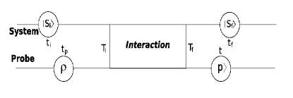
Figure 1: A schematic view of the measurement with pre- and post-selection, the horizontal direction representing increasing time.

At time $t_{f}\geq T_{f}$, a sharp measurement of an observable $\hat{S}_{f}$ of the system is made, giving an outcome $S$, corresponding to the eigenstate $|S\rangle$. At time $t\geq T_{f}$ a sharp measurement of the observable $\hat{p}$ is made on the probe. Since $\hat{p}$ is conserved during the free evolution of the probe, this value will not depend on the time $t$. The observed value of non-conserved quantities, by contrast, would depend on $t$ . Finally, only those trials in which the last measurement on the system gave an arbitrarily fixed outcome $S=S_{f}$ will be selected (postselection). The procedure detailed above describes a measurement with pre- and post-selection. In Fig.(1) we provide a sketch of the procedure.

The joint probability of observing the outcome $p$ for the probe, at any time $t\geq T_{f}$ and $S_{f}$ for the system, at time $t_{f}$, is given by Born’s rule

$$\mathcal{P}(p,S_{f}|\rho,S_{i})=\int dp_{0}dp_{0}^{\prime}e^{i\left[H_{p}(p_{0}^{\prime})-H_{p}(p_{0})\right](T_{i}-t_{p})/\hbar}$$

$$\times\rho(p_{0},p_{0}^{\prime})\langle\tilde{S}_{f}|\langle p|\mathcal{U}_{T_{i},T_{f}}|\tilde{S}_{i}\rangle|p_{0}\rangle\langle\tilde{S}_{i}|\langle p_{0}^{\prime}|\mathcal{U}_{T_{i},T_{f}}^{\dagger}|\tilde{S}_{f}\rangle|p\rangle$$ (1)

where $\mathcal{U}$ is the time evolution operator for $H_{sys}+H_{p}+H_{int}$, we introduced $\rho(p,p^{\prime})$ the probe density matrix in the $|p\rangle$ basis, and $|\tilde{S}_{i,f}\rangle:=\exp{\left\{-i\hat{H}_{sys}(T_{i,f}-t_{i,f})/\hbar\right\}}|S_{i,f}\rangle$. After introducing twice the identity resolved in terms of the eigenstates of $\hat{A}$, we obtain

$$\mathcal{P}(p,S_{f}|\rho,S_{i})= \sum_{a,a^{\prime}}\rho(p-\lambda a,p-\lambda a^{\prime})e^{-i\left[\Phi_{a}-\Phi_{a^{\prime}}\right]}$$

$$\times\langle\tilde{S}_{f}|a\rangle\langle a|\tilde{S}_{i}\rangle\langle\tilde{S}_{i}|a^{\prime}\rangle\langle a^{\prime}|\tilde{S}_{f}\rangle,$$ (2)

with $a,|a\rangle$ the eigenvalues and eigenvectors of $\hat{A}$ and

$$\Phi_{a}:=\frac{1}{\hbar}\int_{t_{p}}^{T_{f}}\!\!\!ds\ H_{p}\!\left(p-\lambda\;a\!\int_{s}^{T_{f}}ds^{\prime}g(s^{\prime})\right).$$ (3)

For an instantaneous interaction, $T_{f}$ in Eq. (3) and elsewhere in this paper should be interpreted as being a time infinitesimally later than the interaction. In deriving Eq. (2), we exploited

$$\langle p|\mathcal{T}\!e^{\!-i\!\int_{0}^{t}\!ds\!\left[H_{p}\!(\hat{p})\!-\!f\!(s)\hat{q}\right]\!/\!\hbar}|p_{0}\rangle =\delta\!\left(p\!-\!p_{0}\!-\!\int_{0}^{t}dsf(s)\right)$$

$$\times\!e^{-i\!\int_{0}^{t}\!ds\!H_{p}\left(\!p\!-\!\int_{s}^{t}\!ds^{\prime}f\!(s^{\prime})\!\right)\!/\!\hbar}.$$ (4)

We notice that if no postselection were made (i.e. if one would sum over the final states $|S_{f}\rangle$), the off-diagonal elements of $\rho(p,p^{\prime})$ would not contribute to Eq. (2).

The conditional probability of obtaining outcome $p$, given that the state has been postselected in $S_{f}$, is

$$\mathcal{P}(p|S_{f},\rho,S_{i})=\frac{\mathcal{P}(p,S_{f}|\rho,S_{i})}{\int dp^{\prime}\mathcal{P}(p^{\prime},S_{f}|\rho,S_{i})},$$ (5)

where we applied Bayes’ rule, and the expected value inferred for the system through observation of the probe

$$\langle A\rangle:=\frac{\langle p\rangle}{\lambda}=\frac{\int\!d\!p\,(p/\lambda)\mathcal{P}(p,S_{f}|\rho,S_{i})}{\int\!d\!p^{\prime}\mathcal{P}(p^{\prime},S_{f}|\rho,S_{i})}.$$ (6)

Since what matters is the deviation of the pointer $p$ from its unperturbed expected value $\int dp\ p\rho(p,p)$, we can set the latter to be zero without loss of generality. We notice that the inference assigning the quantity $A=p/\lambda$ to the system when observing the probe to have the value $p$ is valid only when initially the probe has a precise enough value of $p$ close to zero. We can, however, keep assigning the value to the system even when the probe is not sharply prepared around $p=0$, and say that we observed a value $A$ for the measured system (and correspondingly we shall define a probability $\mathcal{P}(A):=\lambda\mathcal{P}(p/\lambda)$). This value is not necessarily one of the eigenvalues of $\hat{A}$, and, as shown in AAV , it can even lie outside the range $[a_{min},a_{max}]$ (for this reason we are indicating with $a$ the eigenvalues of $\hat{A}$ and with $A$ the outcome of each individual measurement).

III Weak Measurement

A measurement is weak when the coupling $\lambda$ is small compared to the coherence length of the probe, i.e. to the range of $|p-p^{\prime}|$ within which $\rho(p,p^{\prime})$ vanishes. This can be evinced from Eq. (2).

In the following, we shall assume that $\rho(p,p^{\prime})$ is analytic in a neighborhood of $p=p^{\prime}$. Then, to lowest order in $\lambda$, the denominator in Eq.(6) is $\int dp\mathcal{P}(p,S_{f}|\rho,S_{i})=|\langle\tilde{S}_{f}|\tilde{S}_{i}\rangle|^{2}$. Before analysing the numerator in Eq.(6), we rewrite $\rho(p,p^{\prime})=F(p,p^{\prime})\exp{\{i\alpha(p,p^{\prime})\}}$, with $F,\alpha$ symmetric and antisymmetric real functions, respectively. We have then that the numerator in Eq.(6) is

$$\int dp\frac{p}{\lambda}\mathcal{P}(p,S_{f}|\rho,S_{i})\simeq\!-\!\sum_{a,a^{\prime}}\langle\tilde{S}_{f}|a\rangle\langle a|\tilde{S}_{i}\rangle\langle\tilde{S}_{i}|a^{\prime}\rangle\langle a^{\prime}|\tilde{S}_{f}\rangle$$

$$\int dp\ \frac{p}{2}\left\{(a+a^{\prime})\frac{d\mathcal{P}(p)}{dp}-i(a-a^{\prime})\mathcal{P}(p)G(p)\right\}$$

$$= {Re}\!\left(\langle\tilde{S}_{f}|\hat{A}|\tilde{S}_{i}\rangle\langle\tilde{S}_{i}|\tilde{S}_{f}\rangle\right)\!-\!\overline{pG(p)}{Im}\!\left(\langle\tilde{S}_{f}|\hat{A}|\tilde{S}_{i}\rangle\langle\tilde{S}_{i}|\tilde{S}_{f}\rangle\right),$$

where $\mathcal{P}(p):=F(p,p)$ is the initial distribution of the $p$ observable of the probe,

$$G(p)=\frac{2\Delta t}{\hbar}\frac{dH_{p}(p)}{dp}-2\left.\frac{\partial\alpha(p,p^{\prime})}{\partial p}\right|_{p^{\prime}=p},$$

$$\Delta t=\int_{t_{p}}^{T_{f}}ds\int_{s}^{T_{f}}ds^{\prime}g(s^{\prime})\ ,$$ (7)

and the bar symbol denotes the average over $\mathcal{P}(p)$. After introducing the weak value, i.e. the complex number $A_{w}:={\langle\tilde{S}_{f}|\hat{A}|\tilde{S}_{i}\rangle}/{\langle\tilde{S}_{f}|\tilde{S}_{i}\rangle}$, the average value is

$$\langle A\rangle\simeq\langle A\rangle_{0}:={Re}\!\left\{A_{w}\right\}-\overline{pG(p)}\ {Im}\!\left\{A_{w}\right\}.$$ (8)

Eq.(8) holds as far as the product of the prepared and the postselected state is larger than the first nonvanishing contribution in the $\lambda$ expansion for the denominator. In the latter case, one should keep the latter contribution as well.

IV Comparison with previous results

We notice that the contribution of the imaginary part has been generally overlooked in the literature, due to the neglecting of the Hamiltonian of the probe and to the choice of a very special phase $\alpha(p,p^{\prime})=0$. On the other hand, it has been proved AAV ,AV that observing the $\hat{q}$ variable of the probe one gets an average value which is proportional to the imaginary part of $A_{w}$. This is true only if one neglects the time evolution of the probe from preparation to observation. When this evolution is accounted for, the observed value of $\hat{q}$ depends also on the details of the free Hamiltonian of the probe and on the time of observation. To the best of our knowledge, the first paper to point out that ${Im}(A_{w})$ contributes to $\langle A\rangle$ was reference Jozsa . There, however, the readout variable $\hat{p}$ (which in the notation of Jozsa is actually $\hat{q}$) is not conserved during the free evolution of the probe. Thus the results presented in Jozsa hold only if the system-probe interaction is instantaneous, and if the probe is read immediately after the interaction. Indeed, if the interaction is instantaneous, the probe is prepared at time $t_{p}$ and it is observed at time $t$, the central result, Eq.(17), of Ref. Jozsa should be substituted by (we use our notation $\hat{p}\leftrightarrow\hat{q}$)

$$\langle M\rangle\simeq\langle\hat{M}(t)\rangle_{p}+i\lambda\biggl{[}{Re}A_{w}\langle\left[\hat{M}(t),\hat{q}(T_{i})\right]\rangle_{p}$$

$$-{Im}A_{w}\left(\langle\left\{\hat{M}(t),\hat{q}(T_{i})\right\}\rangle_{p}-2\langle\hat{M}(t)\rangle_{p}\langle\hat{q}(T_{i})\rangle_{p}\right)\biggr{]},$$ (9)

where $[\cdot,\cdot]$ ($\{\cdot,\cdot\}$) denotes (anti)commutator, $\langle\hat{M}\rangle_{p}={Tr}\{\hat{\rho}\hat{M}\}$ is the trace taken with the probe density matrix at time $t_{p}$, and $\hat{M}(t)$ is the probe observable $\hat{M}$ evolved with $H_{p}$ in the interval $[t_{p},t]$. Generally, with a probe Hamiltonian $H_{p}=\hat{p}^{2}/2M_{p}+V(\hat{q})$, one can no longer link the contribution of ${Im}\{A_{w}\}$ to $\langle p\rangle$ with the derivative of the variance of $q$, unless $t=T_{i}$. However, if the probe Hamiltonian is $\hat{H_{p}}=\hat{p}^{2}/2M_{p}$, we have that $\hat{p}(t)=\hat{p}(T_{i})$ and thus

$$\langle p\rangle\simeq\lambda{Re}\{A_{w}\}-\lambda\frac{M_{p}}{\hbar}\beta{Im}\{A_{w}\},$$ (10)

where $\beta:=\left.{d{Var}q(t)}/{dt}\right|_{t=T_{i}}$. The formula agrees with the more general Eq. (8), since for a generic $H_{p}(p)$

$$\frac{d{Var}q(t)}{dt}=\hbar\overline{\frac{dH_{p}(p)}{dp}G(p)}-\hbar\overline{\frac{dH_{p}(p)}{dp}}\overline{G(p)},$$

which reduces to ${d{Var}q(t)}/{dt}=\hbar\overline{pG(p)}/M_{p}$. For a generic Hamiltonian $H_{p}(\hat{p})$, if instead of observing $\hat{p}$, one observes the “velocity” operator $\hat{V}=V(\hat{p}):=dH_{p}(\hat{p})/dp$, one has

$$\langle V\rangle\!\simeq\!\langle\hat{V}\rangle_{p}\!+\!\lambda\langle\frac{d\hat{V}}{d\hat{p}}\rangle_{p}{Re}\{A_{w}\}\!-\!\lambda\beta{Im}\{A_{w}\}.$$ (11)

V Probe prepared in a mixed gaussian state

So far, in the literature on the weak measurement, the probe was assumed to be prepared in a pure gaussian state. The corresponding density matrix $\rho(p,p^{\prime})$ is characterized by the identity between the scale in $|p-p^{\prime}|$ over which its off-diagonal elements vanish (the coherence length scale) and the scale over which the diagonal elements decay going away from the zero value (the classical uncertainty spread in $p$). We shall consider a more general gaussian distribution

$$\rho(p,p^{\prime})\!=\!\frac{e^{-\left\{\!(p+p^{\prime})^{2}/8\Delta P^{2}\!+(p-p^{\prime})^{2}/8\delta p^{2}-i\left(p-p^{\prime}\right)/2p_{\phi}\!\right\}}}{\sqrt{2\pi}\Delta P}\!.$$ (12)

Here $\Delta P$ is the initial spread and $\delta p$ the coherence scale. Positive semidefineteness requires $\delta p\leq\Delta P$. We assumed a phase linear in $p$, with $p_{\phi}$ a scale. The linear phase such chosen defines the center of the Wigner function in the coordinate $Q$, $Q_{0}:=\hbar/2p_{\phi}$. We take a quadratic Hamiltonian for the free probe $H_{p}(\hat{p})=\hat{p}^{2}/2M_{p}$, and we define a further scale $p_{H}:=\sqrt{\hbar M_{p}/2\Delta t}$, with $\Delta t$ defined by Eq.(7). We stress that the presence of $\sqrt{\hbar}$ can make this scale the smallest one. We have then that the average detected value of the observable $\hat{A}$ is given by Eq. (8) with $\overline{pG(p)}=\Delta P^{2}/p_{H}^{2}:=\kappa^{2}$. The results of Ref. AAV are recovered for $\Delta P=\delta p$, and $p_{H},p_{\phi}\to\infty$. We also provide an expression for the variance of $A$

$$\langle\Delta A^{2}\rangle\simeq\frac{\Delta P^{2}}{\lambda^{2}} +\frac{1}{2}\left(1-\kappa^{4}\right){Re}\Delta A^{2}_{w}-\kappa^{2}{Im}\Delta A^{2}_{w},$$ (13)

where we introduced $\Delta A^{2}_{w}:=(A^{2})_{w}-(A_{w})^{2}$, with $(A^{2})_{w}:=\langle S_{f}|\hat{A}^{2}|S_{i}\rangle/\langle S_{f}|S_{i}\rangle$. We notice that there is always a large contribution $\Delta P^{2}/\lambda^{2}$, due to the initial spread in $p$. The calculated variance differs from Eqs. (24,25) of Ref. AV : even for $\kappa=0$ (which is the limit considered in AV ), Eq. (13) allows $\langle\Delta A^{2}\rangle<\Delta P^{2}/\lambda^{2}$. We also stress that if the last two terms in Eq.(13) take a small value, this does not imply that a single measurement can reveal the weak value: $A$ is inferred from the observed $p$ of the probe through $A=p/\lambda$; since $p$ has a spread of order $\Delta P$, the value of $A$ observed in each individual measurement will vary with a spread of order $\Delta P/\lambda$, which is large by hypothesis.

VI Illustration: weak measurement of a spin component

As a specific example, we consider a measurement of spin components. We assume that the interaction between the spin and the probe lasts a finite time $T$, that $g(t)=1/T$ during the interaction and zero otherwise, and that the probe is prepared in the state $\rho$ of Eq. (12) immediately before the beginning of the interaction. Then Eq. (7) gives $\Delta t=T/2$. We take the spin to have been preselected in the state up along direction $\mathbf{n}_{i}$ and postselected in the state up along a direction $\mathbf{n}_{f}$, while $\hat{A}=\mathbf{n}\cdot\hat{\boldsymbol{\sigma}}$. Then we obtain from Eqs.(5,2)

$$\mathcal{P}(p|S_{f},\rho,S_{i})=\frac{1}{\sqrt{2\pi}\Delta PN}$$

$$\frac{1}{2}\sum\limits_{\sigma=\pm 1}\Biggl{\{}\left(1+\sigma\mathbf{n}\cdot\mathbf{n}_{i}\right)\left(1+\sigma\mathbf{n}\cdot\mathbf{n}_{f}\right)e^{-(p-\sigma\lambda)^{2}/2\Delta P^{2}}$$

$$+\biggl{[}(\mathbf{n}\!\times\!\mathbf{n}_{i})\cdot(\mathbf{n}\!\times\!\mathbf{n}_{f})\cos{\left[\lambda G(p)\right]}$$

$$-\mathbf{n}\cdot(\mathbf{n}_{i}\!\times\!\mathbf{n}_{f})\sin{\left[\lambda G(p)\right]}\biggr{]}e^{-p^{2}/2\Delta P^{2}-\lambda^{2}/2\delta p^{2}}\Biggr{\}},$$ (14)

$$N=1+\mathbf{n}_{i}\cdot\mathbf{n}_{f}+e^{-\lambda^{2}/2\nu^{2}}\sin{\left(\frac{\lambda}{p_{\phi}}\right)}\mathbf{n}\cdot(\mathbf{n}_{i}\times\mathbf{n}_{f})$$

$$-\left[1-e^{-\lambda^{2}/2\nu^{2}}\cos{\left(\frac{\lambda}{p_{\phi}}\right)}\right](\mathbf{n}\times\mathbf{n}_{i})\cdot(\mathbf{n}\times\mathbf{n}_{f}),$$ (15)

with $\nu:=[1/\delta p^{2}+\kappa^{4}/\Delta P^{2}]^{-1/2}\leq\Delta P/\sqrt{1+\kappa^{4}}$.

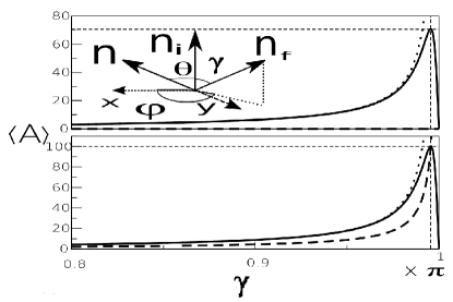
Figure 2: $\langle A\rangle$ as a function of $\gamma$ for $\theta=\pi/2$, and $\phi=\pi/2$ (top figure), $\phi=\phi^{*}=\pi/4$ (bottom figure). (The inset shows how the angles were defined.) The full line depicts the exact value, the dotted one depicts the approximate value including the contribution of ${Im}\{A_{w}\}$, and the dashed line the contribution of ${Re}\{A_{w}\}$. The thin vertical and horizontal lines correspond to $\gamma^{*}=\pi-\lambda/\nu$, $\langle A\rangle_{m}=\epsilon(\phi)\;\nu/\lambda$ [see Eqs.(17,18)]. In the range $\gamma=[0,3]$, the dotted and the full line practically coincide. We assumed $\lambda/\delta p=0.01,\lambda/p_{\phi}=0,\delta p=\Delta P=p_{H}$.

The exact average value is

$$\langle A\rangle= \biggl{\{}\mathbf{n}\!\cdot\!\mathbf{n}_{i}+\mathbf{n}\!\cdot\!\mathbf{n}_{f}-\kappa^{2}e^{-\lambda^{2}/2\nu^{2}}\biggl{[}\cos{\!\left(\!\frac{\lambda}{p_{\phi}}\!\right)}\mathbf{n}\!\cdot\!(\mathbf{n}_{i}\!\times\!\mathbf{n}_{f})$$

$$-\sin{\left(\frac{\lambda}{p_{\phi}}\right)}(\mathbf{n}\!\times\!\mathbf{n}_{i})\cdot(\mathbf{n}\!\times\!\mathbf{n}_{f})\biggr{]}\biggr{\}}\big{/}N.$$ (16)

To lowest order in $\lambda$, $\langle A\rangle$ is given by Eq. (8) with $A_{w}=\mathbf{n}\cdot\left[\mathbf{n}_{i}+\mathbf{n}_{f}+i\mathbf{n}_{i}\!\times\!\mathbf{n}_{f}\right]/\left[1+\mathbf{n}_{i}\cdot\mathbf{n}_{f}\right]$. Interestingly, when $\mathbf{n}$ lies in the plane orthogonal to the bisector of $\mathbf{n}_{i}$ and $\mathbf{n}_{f},$ $A_{w}$ is purely imaginary. This setting of the weak measurement can hence be a testing ground to detect the contribution of the imaginary part.

Without loss of generality, we take $\mathbf{n}_{i},\mathbf{n}$ to define the $XZ$ plane, with the former as the $Z$-axis, and the latter forming an angle $\theta\in[0,\pi]$. The direction $\mathbf{n}_{f}$ is defined by the azimuthal and polar angles $\gamma\in[0,2\pi],\phi\in[0,\pi]$ . Then $A_{w}=\cos{\theta}+\sin{\theta}e^{-i\phi}\tan{(\gamma/2)}$. In Figure 2 we plotted $\langle A\rangle$ as a function of $\gamma$ for fixed $\theta,\phi$. We compare the exact value [Eqs. (16,15)], the approximate value $\langle A\rangle_{0}$ given by Eq. (8), and ${Re}(A_{w})$. For fixed $\theta\neq 0,\pi$, and $\phi$, $\langle A\rangle$ reaches extremal values for $\gamma^{*}=\pi-\eta^{*}$,

$$\eta^{*}\simeq\lambda\frac{\sin{\theta}}{\varepsilon(\phi)}\left[\frac{\textstyle\kappa^{2}}{\textstyle p_{\phi}}\pm\sqrt{\frac{\textstyle\varepsilon(\phi)^{2}}{\textstyle\nu^{2}}+\frac{\textstyle(1+\kappa^{4})\left(\cos{\phi}\right)^{2}}{\textstyle p_{\phi}^{2}}}\right],$$ (17)

with $\varepsilon(\phi):=\cos{\phi}+\kappa^{2}\sin{\phi}$. The extremal value is

$$\langle A\rangle_{m}=\frac{\frac{\textstyle\varepsilon(\phi)^{2}}{\textstyle\lambda}}{\frac{\textstyle\cos{\phi}\;\varepsilon^{\prime}(\phi)}{\textstyle p_{\phi}}\pm\sqrt{\frac{\textstyle\varepsilon(\phi)^{2}}{\textstyle\nu^{2}}\!+\!\frac{\textstyle(1+\kappa^{4})\left(\cos{\phi}\right)^{2}}{\textstyle p_{\phi}^{2}}}},$$ (18)

with the prime meaning differentiation.

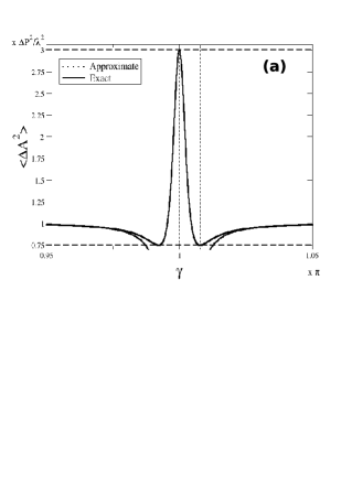
Figure 3: (a) The variance of $A$ as a function of $\gamma$ for fixed $\theta=\pi/2$, $\phi=\pi/4$. The dashed vertical and horizontal lines correspond to the positions and the values of the extrema [Eqs. (20,21)]. (b) The probability distribution for $\theta=\pi/2$, $\phi=\pi/4$ for some significant values of $\gamma$. The parameters are the same as those of Fig. (2).

Generally, the upper sign solution in Eqs. (17,18) holds as far as $\varepsilon(\phi)\gg\lambda/p_{\phi},\lambda/\nu$, in which case the extremum is no longer found close to $\pi$, but

$$\sin{\gamma^{*}}\simeq\frac{-2\kappa^{2}\frac{\lambda}{p_{\phi}}\sin{\theta}\left(\varepsilon(\phi)+\varepsilon^{\prime}(\phi)\frac{\lambda}{p_{\phi}}\cos{\theta}\right)}{\left(\kappa^{2}\frac{\lambda}{p_{\phi}}\sin{\theta}\right)^{2}+\left(\varepsilon(\phi)+\varepsilon^{\prime}(\phi)\frac{\lambda}{p_{\phi}}\cos{\theta}\right)^{2}}\;,$$ (19)

and $\langle A\rangle_{m}\simeq\cos{\theta}$, while the lower sign solution converges to $\eta^{*}\simeq-\lambda\sin{\theta}/p_{\phi}\sqrt{1+\kappa^{4}}$,

$$\langle A\rangle_{m}=-\frac{2\kappa^{2}\lambda/p_{\phi}}{\kappa^{4}\lambda^{2}/(1+\kappa^{4})p_{\phi}^{2}+\lambda^{2}/\nu^{2}}.$$

There are two exceptions to this: (i) For $p_{\phi}\gg\nu$, $\eta^{*}\simeq\pm\sin{\theta}{\lambda}/{\nu}$, and $\langle A\rangle_{m}=\pm\varepsilon(\phi){\nu}/{\lambda}$. (ii) For $\kappa^{2}=2\Delta P^{2}\Delta t/\hbar M_{p}\ll 1$, $\eta^{*}\simeq\pm\sin{\theta}\lambda\sqrt{1/\nu^{2}+1/p_{\phi}^{2}}$, and $\langle A\rangle_{m}\!=\!\cos(\phi)/\lambda\left[\pm\sqrt{1/\nu^{2}+1/p_{\phi}^{2}}-\sin{\phi}/p_{\phi}\right]$.

The extremal value for $\langle A\rangle$ as a function of both $\gamma,\phi$ has an involved expression, except for $p_{\phi}\gg\nu$, when the location of the extremum is $\gamma^{*}=\pi\mp\sin{\theta}\lambda/\nu,\phi^{*}={Arctan}(\kappa^{2})$, and $\langle A\rangle_{m}=\pm\sqrt{1+\kappa^{4}}\nu/\lambda$. In the same limit, we have that the minimum of the spread is reached for $\eta^{*}\simeq\pm\sqrt{3}\sin{\theta}\lambda/\nu,\phi^{*}={Arctan}(\kappa^{2})$

$$\langle\Delta A^{2}\rangle_{min}=\frac{\Delta P^{2}-(1+\kappa^{4})\nu^{2}/4}{\lambda^{2}}\geq\frac{3}{4}\frac{\Delta P^{2}}{\lambda^{2}}.$$ (20)

Its maximum is reached for $\gamma^{*}=\pi$, and it is

$$\langle\Delta A^{2}\rangle_{max}\simeq\frac{\Delta P^{2}+2(1+\kappa^{4})\nu^{2}}{\lambda^{2}}\leq 3\frac{\Delta P^{2}}{\lambda^{2}}.$$ (21)

We plot the probability distribution for three values of $\gamma$: close to $\gamma=\pi$ the distribution has two peaks, each of order $100$ for the choice of parameters made. While the average value goes to zero when $\gamma$ gets very close to $\pi$ ($\pi-\gamma\ll\lambda/\nu$), the probability density of observing a value in the range $[-1,1]$ is rather small: in each individual measurement, it is likely that the value of $|A|$ will be much larger than unity.

VII Conclusions

We have showed that accounting for the dynamics of the probe in the weak measurement leads to an observable deviation of the average value from the real part of the complex weak value defined in Ref. AAV . We have also derived an expression for the spread, and, in the case of spin, we have individuated the locations and values of the extrema of $\langle A\rangle$.

This work was supported by FAPESP and CNPq.

References

(1) Y. Aharonov, D. Z. Albert, and L. Vaidman, Phys. Rev. Lett. 60, 1351 (1988).
(2) I. M. Duck, P. M. Stevenson, and E. C. G. Sudarshan, Phys. Rev. D 40, 2112 (1989).
(3)
N. W. M. Ritchie, J.G. Story, and R. G. Hulet, Phys. Rev. Lett. 66, 1107
(1991);
(4)
A. D. Parks, D. W. Cullin, and D. C. Stoudt, Proc. Roy. Soc. Lon. A 454, 2997 (1998).
(5)
G. J. Pryde, J. L. OBrien,A. G. White, T. C. Ralph, and H. M. Wiseman, Phys. Rev. Lett. 94, 220405
(2005).
(6) N. Brunner, A. Acín, D. Collins, N. Gisin, and V. Scarani, Phys. Rev. Lett. 91, 180402 (2003).
(7) D. R. Solli, C. F. McCormick, R. Y. Chiao, S. Popescu, and J. M. Hickmann,
Phys. Rev. Lett. 92, 043601 (2004).
(8) N. S. Williams and A. N. Jordan, Phys. Rev. Lett. 100, 026804 (2008);
A. Romito, Y. Gefen, and Y. M. Blanter, Phys. Rev. Lett. 100, 056801 (2008).
(9) V. B. Braginsky and F. Ya. Khalili, Quantum Measurement (Cambridge Univ. Press, Cambridge, 1992).
(10) Y. Aharonov and L. Vaidman, Phys. Rev. A 41, 11 (1990).