Solving the Einstein constraint equations
on multi-block triangulations using
finite element methods

Abstract

In order to generate initial data for nonlinear relativistic simulations, one needs to solve the Einstein constraints, which can be cast into a coupled set of nonlinear elliptic equations. Here we present an approach for solving these equations on three-dimensional multi-block domains using finite element methods. We illustrate our approach on a simple example of Brill wave initial data, with the constraints reducing to a single linear elliptic equation for the conformal factor $\psi$. We use quadratic Lagrange elements on semi-structured simplicial meshes, obtained by triangulation of multi-block grids. In the case of uniform refinement the scheme is superconvergent at most mesh vertices, due to local symmetry of the finite element basis with respect to local spatial inversions. We show that in the superconvergent case subsequent unstructured mesh refinements do not improve the quality of our initial data. As proof of concept that this approach is feasible for generating multi-block initial data in three dimensions, after constructing the initial data we evolve them in time using a high order finite-differencing multi-block approach and extract the gravitational waves from the numerical solution.

1 Introduction

This paper is part of an effort to numerically solve Einstein’s equations on general domains with arbitrary shapes and topologies. Accurate simulations on such domains require multiple numerical grids covering different areas of the domain, possibly refined where the solution has interesting features. For the numerical discretization one can use either finite differences (FD), spectral methods, or finite elements (FE). Current research in numerical relativity community is dominated by finite differences methods, not the last reason for that being the relative ease of finite differences implementation and parallelization. A lot of important results in areas of hyperbolic solvers, boundary conditions, domain representation, apparent horizon finders, wave extraction, stability proofs etc., were established and successfully implemented using the FD methods (see [1, 2] and references therein).

Our approach was designed to allow for fast and accurate transformation of the numerical function between FE and FD representations. We demonstrate that the FE solution to an elliptic equation, generated for the given FD grid, is sufficiently accurate and convergent for 3D relativistic simulations with independent finite difference hyperbolic solver (QUILT).

Spectral methods are also widely used [3, 4], mainly for solving elliptic equations, such as those arising in initial value problems [5, 6, 7, 8, 9], constrained evolution [10] and apparent horizon finders [11, 12]. They can as well be applied to hyperbolic problems [13], as in the recent very successful simulations of the binary black holes merger [14] (using an approach, developed by the Cornell-Caltech collaboration [15, 16, 17, 18]). Spectral methods can produce exceptionally accurate results, but in order to use these results in a FD evolution code one needs to perform an additional interpolation step. The interpolation can be too slow for some applications, for instance, in constrained evolution schemes. In our approach, the interpolation is trivial, and the number of degrees of freedom on FE and FD grid is the same, which allows to exchange solution between the FE and FD solvers without reducing its accuracy by interpolation. Another advantage of FE methods compared to spectral methods is that the matrices resulting from FE discretizations are sparse.

Finite element methods can also be applied to hyperbolic problems, however, stable and accurate discretizations require using discontinuous Galerkin (DG) flavor of finite elements (otherwise the approximation is suboptimal: order of convergence falls to $(p-1)$ and the solution is not necessarily stable).

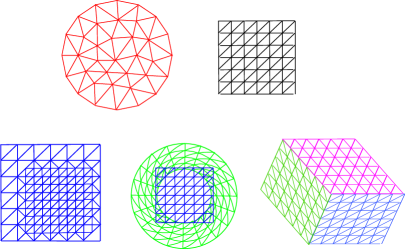
Figure 1: Types of FE meshes. Top left: unstructured mesh, top right: regular mesh, bottom: semistructured meshes.

In this paper, the term grid is used in reference to the finite differences grid (an ordered set of points), as opposed to the term mesh for the finite element triangulation. Domain triangulations can be classified as regular, unstructured or semistructured, depending on their degree of symmetry (see figure 1). Finite element methods can handle domains of arbitrarily complex shapes and topologies, since every geometrical shape admits approximation with succesively refined unstructured symplectic triangulations. However, the domains encountered in numerical relativity are relatively simple in the sense that they can be covered with semistructured meshes. We argue in favor of using semistructured meshes over unstructured ones. One of the motivations is that they can be quickly constructed on top of existing FD grids without the need to explicitly maintain all the information about mesh elements, such as edges, faces etc. Raising the order of finite elements, one can essentially achieve the spectral convergence; however, here we concentrate on lower-order finite elements (first- and second-order), and show how the superconvergence on semistructured grids for second-order elements can be exploited to obtain accurate 4-th order convergent solution, suitable for use in finite differences simulation.

The method is tested on the particular example of multipatch FD grid. In differential geometry it is common to define a manifold through a set of possibly overlapping patches, with each patch mapped into an open, simply-connected subset of Euclidean space (see, for example, [19]). This is a natural way of describing manifolds with nontrivial topology, which cannot be covered by a single coordinate chart. After discretization every chart becomes a FD grid, which can be thought of as a discrete coordinate chart, mapped into a region of $\mathbb{Z}^{3}$. At the continuum level, the patches are glued together by coordinate transformations in the areas where they intersect. At the discrete level, if the neighboring patches do not have common points interpolation can be used to fill in the missing ones; this approach is commonly referred to as overlapping-grids. On the other hand, in a multi-block approach the patches abut rather than overlap, and the grids are constructed in such a way that neighboring grids share boundary points.

A multipatch approach in numerical relativity has several advantages. In many cases the domain of interest is asymptotically flat. If it contains one or more black holes, then each hole can be excised from the computational domain by introducing an inner smooth boundary around the singularity. If appropriately chosen, this boundary does not require any physical boundary conditions, since all characteristic modes leave the domain. It is preferable that this boundary is smooth, which in general requires the use of multiple patches. Similarly, the preferred shape for the outer boundary when simulating asymptotically flat spacetimes is a sphere, as this is the topology of null infinity $\mathcal{J}^{+}$, which is best suited for extracting gravitational waves. A multipatch domain structure easily accomodates both type of boundaries while avoiding coordinate singularities, such as those associated with spherical or cylindrical coordinates. The use of multiple patches is unavoidable in cosmological simulations with non-trivial topologies. In addition, multiple patches are in general more efficient than regular grids, since they decouple different spatial directions. For example, under conditions of approximate spherical symmetry, one could surround the system with spherical patches and fix the number of points in angular direction, while increasing the domain only in radial direction. This way, pushing the outer boundary out becomes an order $N$ problem, as opposed to $N^{3}$ with Cartesian grids. This same feature makes them useful, in particular, for many relativistic astrophysical studies which are assumed to be approximately spherically symmetric [20].

Einstein’s equations are often written in a form such that the equations divide into hyperbolic (evolution) and elliptic (constraint) sub-systems. When solving the Einstein vacuum (that is, in the absence of matter) evolution equations, these can be cast in linearly-degenerate form, and the solutions are in general expected to be smooth. Those cases are ideally suited for high order or spectral methods. When including matter, on the other hand, for example when dealing with the general relativistic hydrodynamics equations, shocks are expected. In those cases a possible choice is high resolution shock capturing methods [21, 22] adapted to the presence of several patches for the hydrodynamical sub-system and high order or spectral methods for the metric sub-system [20, 23].

This paper is concerned with the elliptic sector of Einstein’s equations, more precisely with the generation of initial data needed for evolutions on multipatch geometries. Initial data on a spacelike hyperslice has to satisfy a set of Enistein’s constraints, which can be cast into a coupled nonlinear elliptic system of partial differential equations (PDE). This elliptic PDE system has been studied extensively for many years, with a complete solution theory developed in the case of domains which are closed (i.e. compact without boundary) 3-manifold spatial slices of spacetime with constant or nearly-constant mean extrinsic curvature [24, 25]. More recently, this solution theory has been extended to both closed 3-manifolds and to compact 3-manifolds with boundary, having mean extrinsic curvature far from constant [26, 27, 28]. It has also been shown recently [29, 30, 31] that geometric partial differential equations of this type can be solved accurately and efficiently using adaptive finite element methods on manifolds with general topologies. For general multi-block systems, the additional structure allows one to construct semi-structured triangulations, which generate superconvergent finite element solutions. The property of superconvergence holds at the vertices of the multi-block grid triangulation, which simplifies transport of the solution to the finite difference grid, since no interpolation is required.

The above considerations define the approach of this paper, which involves solving the Einstein constraint equations on semi-structured multi-block triangulations using finite element methods. We apply this approach to the Brill wave initial data problem, which represents a linear vacuum case with zero extrinsic curvature, with the constraints system reducing to a single elliptic equation $\Delta\psi-V\psi=0$ for the conformal factor $\psi$ (where $\Delta$ is the flat 3-dimensional laplacian and V is a potential function related to the Ricci scalar of the freely given metric). Nevertheless, the results presented are expected to hold in general case, because the property of superconvergence is the property of the mesh and the finite element spaces used. If this property holds for a linearized problem, it is also expected to hold for the full nonlinear one (see Chapter 9 of [32]).

The paper is organized as follows. Section 2 gives an overview and summary of the Finite Element Toolkit (FETK) [29], which we here use for solving the Einstein constraint equations with finite element methods. Section 3 discusses our approach to multi-block triangulations and, in particular, why superconvergence is expected. In section 4 we evaluate the accuracy of our approach by solving for several three-dimensional elliptic test problems on multi-block domains with known exact solutions. Finally, in section 5 we solve the Einstein constraints on a multi-block domain for the case of Brill waves. After constructing initial data, we use the multi-patch infrastructure QUILT to solve for the Einstein evolution equations in time and extract gravitational waves from the numerical solution. QUILT is an ongoing effort, more details of which can be found in [33], [34], [35], [36], [37], [20]. In tensor notations, used throughout the paper, Latin indices from the beginning of the alphabet ($a$,$b$,…) run from 0 to 3, Latin indices $i$, $j$, etc. run from 1 to 3, and the usual Einstein summation rule is assumed.

2 Solving elliptic PDEs using the Finite Element ToolKit

In this paper we use the Finite Element ToolKit (FETK) [29] (see also [38, 31]) to solve the Einstein constraint equations. FETK is an adaptive multilevel finite element code developed over a number of years by the Holst research group at UC San Diego and their collaborators (see also [39]). It is designed to produce provably accurate numerical solutions to nonlinear elliptic systems of tensor equations on (Riemannian) multi-dimensional manifolds in an optimal or nearly-optimal way. We will summarize the main features of FETK here; more detailed discussions of its use for general geometric PDE may be found in [29, 30], and specific application to the Einstein constraint equations may be found in [31, 40].

FETK contains an implementation of a “solve-estimate-refine” algorithm, employing inexact Newton iterations to treat non-linearities. The linear Newton equations at each inexact Newton iteration are solved with unstructured algebraic multilevel methods which have been constructured to have optimal or near-optimal space and time complexity (see [41, 42]). The algorithm is supplemented with a continuation technique when necessary. FETK employs a posteriori error estimation and adaptive simplex subdivision to produce provably convergent adaptive solutions (see [43, 44]).

Several of the features of FETK are somewhat unusual, some of which are:

• Abstraction of the elliptic system: The elliptic system is defined only through a nonlinear weak form along with an associated linearization form over the domain manifold. To use the a posteriori error estimator, a third function $F(u)$ must also be provided (essentially the strong form of the problem).

• Abstraction of the domain manifold: The domain manifold is specified by giving a polyhedral representation of the topology, along with an abstract set of coordinate labels of the user’s interpretation, possibly consisting of multiple charts. FETK works only with the topology of the domain, the connectivity of the polyhedral representation.

• Dimension independence: The same code paths are taken for two-, three- and higher-dimensional problems. To achieve this dimension independence, FETK employs the simplex as its fundamental geometrical object for defining finite element bases.

2.1 Weak Formulation Example

We give a simple example to illustrate how to construct a weak formulation of a given PDE. Here we assume the 3–metric to be flat so that $\nabla$ is the ordinary gradient operator and $\cdot$ the usual inner product. Let $\mathcal{M}$ represent a connected domain in $\mathbb{R}^{3}$ with a smooth orientable boundary $\partial\mathcal{M}$, formed from two disjoint 2-dimensional surfaces $\partial_{0}\mathcal{M}$ and $\partial_{1}\mathcal{M}$.

Consider now the following semilinear equation on $\mathcal{M}$:

$$-\nabla\cdot(a(x)\nabla u(x))+b(x,u(x)) = 0~{}\text{~{}in~{}}\mathcal{M},$$ (2.1)

$$n(x)\cdot(a(x)\nabla u(x))+c(x,u(x)) = 0~{}\text{~{}on~{}}\partial_{1}\mathcal{M},$$ (2.2)

$$u(x) = f(x)~{}\text{~{}on~{}}\partial_{0}\mathcal{M},$$ (2.3)

where $n(x):\partial\mathcal{M}\mapsto\mathbb{R}^{3}$ is the unit normal to $\partial\mathcal{M}$, and where

$$a:\mathcal{M}\mapsto\mathbb{R}^{3\times 3}, b:\mathcal{M}\times\mathbb{R}\mapsto\mathbb{R},$$ (2.4)

$$c:\partial_{1}\mathcal{M}\times\mathbb{R}\mapsto\mathbb{R}, f:\partial_{0}\mathcal{M}\mapsto\mathbb{R}.$$ (2.5)

If the boundary function $f$ is regular enough so that $f\in H^{1/2}(\partial_{0}\mathcal{M})$, then from the Trace Theorem [45], there exists $\bar{u}\in H^{1}(\mathcal{M})$ such that $f=\bar{u}|_{\partial_{0}\mathcal{M}}$ in the sense of the Trace operator (where $H^{1}(\mathcal{M})$ is the Hilbert space of all real $L_{2}$-integrable functions on $\mathcal{M}$ with $L_{2}$-integrable weak derivative [46].) Employing such a function $\bar{u}\in H^{1}(\mathcal{M})$, the weak formulation has the form:

$$\text{~{}Find~{}}u\in\bar{u}+H_{0,D}^{1}(\mathcal{M})~{}\text{~{}s.t.~{}}\langle F(u),v\rangle=0,~{}~{}\forall~{}v\in H^{1}_{0,D}(\mathcal{M}),$$ (2.6)

where the nonlinear form is defined as:

$$\langle F(u),v\rangle=\int_{\mathcal{M}}\left(a\nabla u\cdot\nabla v+b(x,u)v\right)~{}dx+\int_{\partial_{1}\mathcal{M}}c(x,u)v~{}ds.$$ (2.7)

The “weak” formulation of the problem given by equation (2.6) imposes only one order of differentiability on the solution $u$, and only in the weak or distributional sense. Under suitable growth conditions on the nonlinearities $b$ and $c$, it can be shown that this weak formulation makes sense, in that the form $\langle F(\cdot),\cdot\rangle$ is finite for all arguments, and further that there exists a (potentially unique) solution to (2.6). In the specific case of the individual and coupled Einstein constraint equations, such weak formulations are derived and analyzed in [26, 27].

To analyze linearization stability, or to apply a numerical algorithm such as Newton’s method, we will need the bilinear linearization form $\langle DF(u)w,v\rangle$, produced as the formal Gateaux derivative of the nonlinear form $\langle F(u),v\rangle$:

$$\langle DF(u)w,v\rangle=\left.\frac{d}{d\epsilon}\langle F(u+\epsilon w),v\rangle\right|_{\epsilon=0}$$

$$=\int_{\mathcal{M}}\left(a\nabla w\cdot\nabla v+\frac{\partial b(x,u)}{\partial u}wv\right)~{}dx+\int_{\partial_{1}\mathcal{M}}\frac{\partial c(x,u)}{\partial u}wv~{}ds.$$ (2.8)

Now that the nonlinear weak form $\langle F(u),v\rangle$ and the associated bilinear linearization form $\langle DF(u)w,v\rangle$ are defined as integrals, they can be evaluated using numerical quadrature to assemble a Galerkin-type discretization involving expansion of $u$ in a finite-dimensional basis.

As was the case for the nonlinear residual $\langle F(\cdot),\cdot\rangle$, the matrix representing the bilinear form in the Newton iteration is easily assembled, regardless of the complexity of the bilinear form $\langle DF(\cdot)\cdot,\cdot\rangle$. In particular, the algebraic system for $w=\sum_{j=1}^{n}\beta_{j}\phi_{j}$ has the form:

$$AU=F,\ \ \ \ \ U_{i}=\beta_{i},$$ (2.9)

where

$$A_{ij} = \langle DF(\bar{u}_{h}+\sum_{k=1}^{n}\alpha_{k}\phi_{k})\phi_{j},\psi_{i}\rangle,$$ (2.10)

$$F_{i} = \langle F(\bar{u}_{h}+\sum_{j=1}^{n}\alpha_{j}\phi_{j}),\psi_{i}\rangle.$$ (2.11)

and $\{\phi_{i}\}_{i=1}^{N}$, $\{\varphi_{j}\}_{j=1}^{N}$ are the bases of the test and trial $N$-dimensional finite element spaces. As long as the integral forms $\langle F(\cdot),\cdot\rangle$ and $\langle DF(\cdot)\cdot,\cdot\rangle$ can be evaluated at individual points in the domain, then quadrature can be used to build the Newton equations, regardless of the complexity of the forms. This is one of the most powerful features of the finite element method, and is exploited by FETK to make possible the representation and discretization of very general geometric PDEs on manifolds. It should be noted that there is a subtle difference between the approach outlined here (typical for a nonlinear finite element approximation) and that usually taken when applying a Newton-iteration to a nonlinear finite difference approximation. In particular, in the finite difference setting the discrete equations are linearized explicitly by computing the Jacobian of the system of nonlinear algebraic equations. In the finite element setting, the commutativity of linearization and discretization is exploited; the Newton iteration is actually performed in function space, with discretization occurring “at the last moment.”

3 Generating semi-structured multi-block triangulations with superconvergent properties

In order to avoid the extra step of interpolating the finite element numerical solution to a multi-block grid, we use finite element meshes with vertices located at the multi-block grid points. We construct such meshes by dividing a convex hull of the set of grid points into simplices with vertices only at those points. This procedure of building a simplicial mesh based on a set of points is usually referred to as triangulation. Delaunay’s triangulation (see, for instance, [47]) is an example of such a procedure, generating meshes with simplices of the highest possible quality in flat space. Although Delaunay’s triangulation minimizes a condition number in a resulting linear system, it is mostly used for sets of points of general position since it generates completely unstructured meshes; for more regular grids its algorithm is unnecessarily complex. Here we use a simpler and more straightforward algorithm to generate semi-structured meshes with the additional advantage of having superconvergent properties.

The term superconvergence applies in various contexts, when the local or global convergence order of a numerical solution is higher than one would expect [48, 49, 32, 50]. The type of superconvergence we are interested in is superconvergence by local symmetry [32], which occurs in function values for discretizations of second order elliptic boundary value problems, and amounts to an additional $0<\sigma\leq 1$ in the convergence order. It occurs at any given point in which the finite element basis is locally symmetric, or approximately symmetric, with respect to local spatial inversion at that point (see figure 2). The triangulation method that we use produces simplicial meshes with this type of symmetry at all vertices inside each block, and at some vertices at the interblock boundaries. Therefore, in our meshes we expect superconvergence everywhere but at the non-symmetric interblock boundary points. For second order elliptic equations and piecewise polynomial finite elements of even degree superconvergence occurs in the solution itself, while for odd degree it occurs in the first derivatives of the solution [51, 52].

Figure 2: Example of two-dimensional simplectic mesh, locally symmetric with respect to the point  [51].

With this in view, the quadratic Lagrange finite elements at the nodal points of the meshes that we use are expected to give solutions with convergence order $3+\sigma$ (for some $0<\sigma\leq 1$). This is an important advantage of multi-block triangulations: the resulting grid solutions have a convergence rate which is even higher than the global convergence rate of the original finite element solution, almost everywhere.

We start by dividing a cell, then combine cells into a block, and finally combine blocks together in a conforming way. Next we explain how these procedures are performed. The main complexity in building multi-block triangulations comes from the last step, since triangulations of each block are not necessarily conforming at their interfaces. We will show, however, that our method guarantees conforming simplicial triangulations.

Cell triangulation. For a cubical cell, there exist two possible triangulations (see figure 3): the cell can be divided into either five or six tetrahedra. The former is known as middle cut triangulation [53], and the latter as Kuhn’s triangulation [54]. While Kuhn’s triangulation produces simplices of equal shape and can be more easily extended to an arbitrary number of dimensions [55], the middle cut triangulation produces higher quality tetrahedra, in the sense that their angles are less acute than in a Kuhn triangulation, which produces to a finite element matrix system with better condition number. Usually, the quality of tetrahedra is described by the ratio $R/3r$ of radii of circumscribed ($R$) to inscribed ($r$) spheres. For a middle cut triangulation the central tetrahedron has, obviously, minimum possible aspect ratio $R/3r=1$, while for corner tetrahedra we have $R/3r=\frac{1+\sqrt{3}}{2}\approx 1.37$. At the same time, in Kuhn’s triangulation all tetrahedra have aspect ratio $1+1/\sqrt{3}\approx 1.58$.

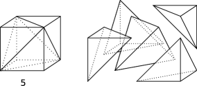
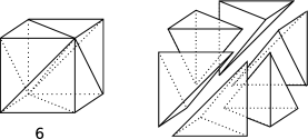
Figure 3: Middle cut triangulation and Kuhn’s triangulation: dividing a cube into five or six tetrahedra, respectively.

Block triangulation. A block can be triangulated in many possible ways. We will consider the two most straightforward and symmetric ones, referring to them as uniform and clustered block triangulations. Both types of triangulation are locally symmetric with respect to local space inversion at any inner vertex of the mesh. In uniform block triangulation, exactly the same cell triangulation, with the same orientation, is applied to all cells in a block (see figure 4). This produces a conforming mesh for Kuhn’s triangulation, but fails to produce a conforming one for the middle cut one, since the triangulation patterns between neighboring cell interfaces are not compatible.

Figure 4: Uniform (left) and clustered (right) block triangulations. With Kuhn’s triangulation of each cell, both types of block triangulation can be done in conforming way for neighboring cells. Cells, triangulated by middle cut, can only be arranged into clustered configuration.

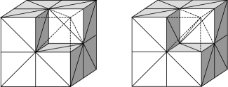
Figure 5: Union jack triangulation of $2\times 2\times 2$-cell cluster. The triangulation pattern on each side of the cluster is the same. Inside, each cluster can have either middle cut (left) or Kuhn (right) triangulations.

To handle this compatibility problem, it is convenient to group neighboring cells into $2\times 2\times 2$ clusters and triangulate each cluster as shown in figure  5, with ”union jack” patterns on each side. This guarantees conformity between neighboring clusters. We will label this type of triangulation as clustered block triangulation. It can be used with both types of cell triangulation.

Multi-Block triangulation. In a multi-block system, both uniform and clustered triangulations of each block can be arranged into a conforming simplicial mesh. Obviously, clustered triangulations of each block with even number of cells on the interfaces between the blocks assemble themselves in a conforming manner. A uniform triangulations arrangement can be constructed from clustered triangulation of the same system by first removing and then replicating layers of cells with Kuhn’s triangulation. Two different types of semi-structured multi-block triangulations, used in this paper, are shown in figure 6.

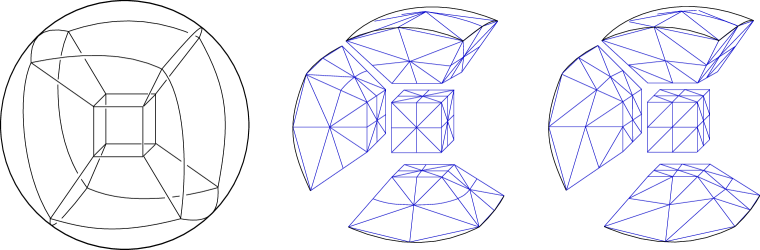
Figure 6: Seven-block system for the sphere (left), and its triangulations, generated using clustered (center) and uniform (right) block triangulations.

4 Quality of our finite element solutions on semi-structured multi-block triangulations

In this section we perform a numerical study of the quality of our finite element solutions obtained using semi-structured multi-block triangulations. We investigate not only the solution itself, but also answer the question of whether this solution is appropriate for finite-difference evolution codes with high-order numerical derivative operators. After introducing the domain structure and weak formulation of the second-order elliptic equation, we evaluate the solution convergence order, and show superconvergence for quadratic finite elements. Then we evaluate the finite element solution at the multi-block gridpoints, apply various high-order finite difference operators and check the convergence orders of its first and second numerical derivatives. The observed convergence orders are consistent with the expected values.

4.1 Domain structures

Both FETK and QUILT were developed to handle equations on general manifolds, with an arbitrary number of charts. However, for the domain structures considered in this paper we can embed the computational domain into a reference Euclidean 3-dimensional space with a single fixed Cartesian system of coordinates to label all vertices and nodes of the mesh, and we do so. The domain of interest here will then be a spherical domain of radius $R$, equipped with a seven-blocks or thirteen-blocks system (see figure 7), with local patch coordinate transformations defined as in [35], [34].

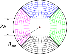
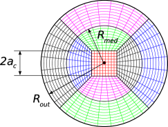
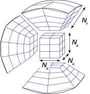
(a)	(b)	(c)

Figure 7: An equatorial cut of (a) seven-block and (b) thirteen-block systems. (c) Grid dimensions for the seven-block system.

The seven-block geometry (see figure 7) is fully specified by fixing the outer sphere radius $R_{out}$ and the side of the inner cubical patch $a_{c}$. In the innermost, cubical patch, there are $N_{x}\times N_{y}\times N_{z}$ points, where $N_{x}=N_{y}=N_{z}:=N$. Since the grids are conforming, in the six blocks surrounding the inner one there are $N\times N\times N_{r}$ points. The thirteen-block geometry, in turn, can be seen as a seven-block one of radius $R_{med}$ and $N\times N\times N_{r,in}$ points, surrounded by six additional blocks with $N\times N\times N_{r,out}$ points each, with a total radius $R_{out}$. The advantage of the thirteen-block setup is that the transversal grid layers in the outermost system are perfectly spherical surfaces. These are very convenient in certain applications which require integration over such surfaces, as in the the study of the multipole structure of radiation in the wave zone (see, for example, [37]), since no interpolation is needed for those integrations (resulting in both higher accuracy and speed). Throughout this paper, when we change the resolution we keep the ratios $N:N_{r}$ and $N:N_{r,in}:N_{r,out}$ in the seven- and thirteen-block systems, respectively, fixed. Multiple domains with different values of $N$ produce a sequence of domain triangulations {$\mathcal{T}_{h}$} with maximal simplex diameters $h$ inversely proportional to $N$. Therefore, it is convenient to use $N$ as a scaling factor in convergence tests, and we do so.

4.2 Second-order elliptic equation and its weak form

Let $S_{R}$ represent our spherical domain with radius $R$, centered at the origin, and let $\partial S_{R}$ be its outer boundary. The equations of interest in this paper are of the form:

$$-\nabla^{2}\psi(\bar{x})+V(\bar{x})\psi(\bar{x}) = 0~{}\text{~{}in~{}}S_{R},$$ (4.1)

$$\psi(\bar{x}) = \psi_{D}~{}\text{~{}on~{}}\partial S_{R}$$ (4.2)

where $\psi_{D}$ is a Dirichlet boundary condition, and $\nabla^{2}$ is the Laplace operator. We only consider the case when both the potential $V$ and the boundary conditions $\psi_{D}$ are axisymmetric. Following the weak formulation example above (section  2.1), we obtain the nonlinear weak form and the bilinear linearization form:

$$\langle F(\psi),\phi\rangle = \int_{S_{R}}\left(\nabla\psi\cdot\nabla\phi+\psi V\phi\right)~{}dx$$ (4.3)

$$\langle DF(\psi)\chi,\phi\rangle = \int_{S_{R}}\left(\nabla\chi\cdot\nabla\phi+\chi V\phi\right)~{}dx$$ (4.4)

with $\psi(\bar{x})\in\bar{\psi}+H^{1}_{0}(S_{R})$, and $\phi(\bar{x})~{},~{}\chi(\bar{x})\in H^{1}_{0}(S_{R})$ as discussed in section 2. These two forms and the Dirichlet boundary function are everything we need to specify the problem in FETK.

We also consider the same problem with more complex Robin boundary conditions:

$$\partial_{r}\psi(\bar{x})=\frac{1-\psi(\bar{x})}{r}~{}\text{~{}on~{}}\partial S_{R}\,,$$ (4.5)

which has the following nonlinear weak and bilinear linearization forms,

$$\langle F(\psi),\phi\rangle = \int_{S_{R}}\left(\nabla\psi\cdot\nabla\phi+\psi V\phi\right)~{}dx+\frac{1}{R}\int_{\partial S_{R}}(\psi-1)\phi~{}ds$$ (4.6)

$$\langle DF(\psi)\chi,\phi\rangle = \int_{S_{R}}\left(\nabla\chi\cdot\nabla\phi+\chi V\phi\right)~{}dx+\frac{1}{R}\int_{\partial S_{R}}\chi~{}\phi~{}ds$$ (4.7)

where now $\psi(\bar{x}),~{}\phi(\bar{x}),~{}\chi(\bar{x})~{}\in~{}H^{1}(S_{R})$. We will use these Robin boundary conditions when solving for Brill waves below in section 5.

4.3 Testing convergence of the solution

As a test problem for our approach to solving elliptic equations on a semi-structured grid using finite elements, we solve equation (4.1) with three different potentials:

$$V_{A} =-3\omega^{2},$$

$$V_{B}(r) =\frac{2(r^{2}-3r_{0}^{2})}{(r^{2}+r_{0}^{2})^{2}},$$

$$V_{C}(\rho,z) =-\frac{2}{Z}\left(1+\frac{4z^{2}}{R}(S+\frac{\sigma_{r}r_{0}^{2}}{Z})\right)+\frac{2(2C+3S)}{R}+2\left(\frac{2rS}{R}\right)^{2},$$

where $R=r^{2}-\sigma_{r}r_{0}^{2}\cosh{\frac{r^{2}}{r_{0}^{2}}}$, $Z=z^{2}+\sigma_{z}^{2}$, $C=\sigma_{r}\cosh{\frac{r^{2}}{r_{0}^{2}}}$, $S=\sigma_{r}\sinh{\frac{r^{2}}{r_{0}^{2}}}-1$.

These are such that they produce the following solutions:

• Plane wave: $\psi_{A}(x,y,z)~{}=~{}\cos(\omega x)\cos(\omega y)\cos(\omega z)$

• Spherically-symmetric pulse with width $r_{0}$, concentrated at the origin, falling off with order $1/r^{2}$ as $r\to\infty$: $\psi_{B}(r)~{}=~{}\frac{1}{1+r^{2}/r_{0}^{2}}$

• Toroidal solution, with radius $\sim r_{0}$ and width $\sim\sigma_{r}$ in the radial direction and $\sigma_{z}$ in the vertical one: $\psi_{C}(\rho,z)=(\cosh{(\frac{r^{2}}{r_{0}^{2}})}-\frac{r^{2}}{\sigma_{r}r_{0}^{2}})^{-1}(1~{}+~{}z^{2}/\sigma_{z}^{2})^{-1}$

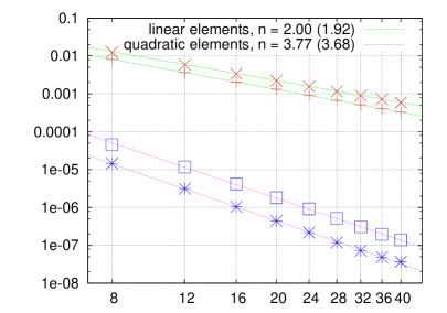
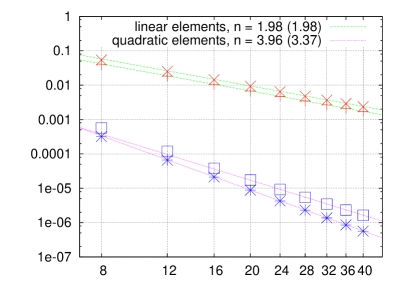
(a)	(b)

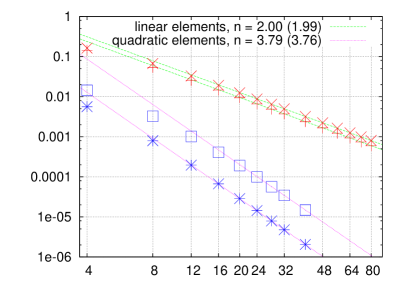
(c)

Figure 8: Convergence of the solution error, in the $l_{2}$ and $l_{\infty}$ norms, with respect to the number of points $N$, for linear and quadratic finite elements. The plots (a), (b) and (c) correspond to the potentials $V_{A}$, $V_{B}(r)$ and $V_{C}(\rho,z)$, respectively. From each pair of lines, the upper one represents the $l_{\infty}$ norm, and the lower one the $l_{2}$ norm. Each plot shows the convergence orders $n$, obtained by linear fit using the four points with highest resolution. The numbers in brackets give the convergence orders in the $l_{\infty}$ norm.

These three potentials are chosen such that the solution for $\psi$ is known in closed form, and they all differ in the way they are adapted to the underlying multi-block grid. The first potential, $V_{A}$, represents a simple periodic wave, with the mesh not adapted to the shape of the wave. Second potential is supposed to model a situation where the wave is concentrated near the origin, in the central cubical patch of the ”cubed sphere” domain. In this case, the grid resolution is adapted to the solution, but not the coordinate lines. Finally, for the potential $V_{C}$ (which has toroidal shape), both the resolution (in the $\theta$ and $r$ directions), and coordinate lines (in $\varphi$ direction) are adapted to the solution.

All the test problems were solved on the same 7-patch spherical domain, with dimensions $R_{out}~{}=~{}10$, $a_{c}~{}=~{}2.5$, and fixed grid size ratios $N~{}:~{}N_{r}~{}=~{}1~{}:~{}2$. The test problems used the following set of parameters: for $V_{A}$: $\omega=0.1$, for $V_{B}(r)$: $r_{0}=4$, and for $V_{C}(\rho,z)$: $r_{0}=8$, $\sigma_{r}=1.2$, $\sigma_{z}=4$.

It is well-known (see, for example, [56], [57], [58]) that in case of the optimal approximation, the convergence rate of continuum-level error norms, $||u_{h}-u_{e}||_{2}$ and $||u_{h}-u_{e}||_{\infty}$, defined in a usual manner,

$$||u_{h}-u_{e}||_{2} = \left(\int_{\mathcal{M}}(u_{h}(x)-u_{e}(x))^{2}dx\right)^{1/2},$$ (4.8)

$$||u_{h}-u_{e}||_{\infty} = \max_{x\in\mathcal{M}}|u_{h}(x)-u_{e}(x)|$$ (4.9)

for the standard uniform refinement, is determined by the approximation power of the finite element function spaces (here, $u_{e}(x)$ is the exact solution, $u_{h}(x)$ is its finite element approximation, and index $h$ denotes the maximum simplex diameter in the domain triangulation $\mathcal{T}_{h}$). If piecewise polynomials of fixed order $p$ are used, then the order of convergence of the continuum-level error norms is $p+1$.

In order to measure the error of the grid solutions, we use discrete $l_{2}$ and $l_{\infty}$ norms, sampled at the nodes and normalized by the corresponding norm of $u_{e}$:

$$\epsilon_{h,2}=\frac{\left(\frac{1}{N}\sum_{k=1}^{N}(u_{h,k}-u_{e}(x_{k}))^{2}\right)^{1/2}}{\left(\frac{1}{N}\sum_{k=1}^{N}u_{e}(x_{k})^{2}\right)^{1/2}} \epsilon_{h,\infty}=\frac{\max_{k}|u_{h,k}-u_{e}(x_{k})|}{\max_{k}|u_{e}(x_{k})|}$$

The plots on figure 8 show the convergence of $\epsilon_{h,2}$ and $\epsilon_{h,\infty}$ with $N$ ($N$ is inversely proportional to the maximum mesh diameter $h$, see section 4.1). Note that the convergence orders in the $l_{2}$ and $l_{\infty}$ norms agree, which means that the pointwise convergence order is the same everywhere. The observed convergence order for linear elements is $2$, which is supposed to be the case, since the order of piecewise polynomials is odd. For quadratics, we expect to have superconvergence, and indeed, the observed convergence rate is $\approx 4$.

4.4 Testing convergence of numerical derivatives of the solution

To set up initial data for our General Relativity evolution codes, we need not only the solution itself but also its first spatial derivatives, because we use a first-order formulation of the Einstein evolution equations. In total, our finite element solution has to be differentiated twice: once, when setting initial data, and one more time when computing the evolution equations. In this subsection we numerically study how our obtained finite element solutions behave under two numerical finite-difference differentiations in terms of convergence.

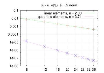
(a)

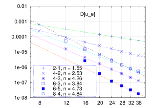
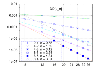
(b)

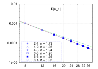
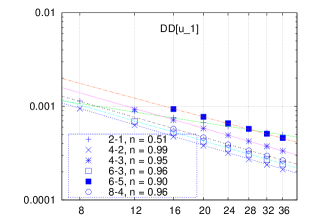
(c)

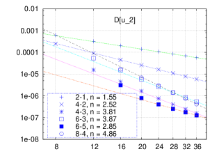
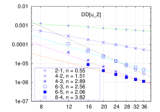
(d)

Figure 9: (a) Convergence of the solution error in the $l_{2}$-norm, for linear and quadratic finite elements, for the test problem with potential $V_{A}$ and $\omega=0.1$. (b,c,d) Convergence in the $l_{2}$-norm of the first (left) and second (right) numerical FD derivatives of: (b) the exact solution, restricted to the FD grid; (c) the numerical solution obtained using linear finite elements; (d) the numerical solution obtained using quadratic finite elements. In all cases several FD operators are used to compute the derivatives, and the resulting convergence factors (denoted by $n$) are shown

If we were using completely unstructured meshes and interpolated the finite element solution to the multi-block grids used in our evolutions, the resulting grid solution would have an error of order $O(h^{p+1})$. Two numerical differentiations in this case would take away two orders of convergence, leading to an unacceptable low convergence order. However, as discussed above, when using semi-structured grids special conditions which lead to superconvergence can be met, and the convergence rate of numerical derivatives improve.

The procedure for converting the finite element solution into the grid solution is trivial: the value of the solution $u(x)=\sum_{i=1}^{N}c_{i}\phi_{i}(x)$ at a node $i$ is simply the corresponding nodal coefficient $c_{i}$. In order for the nodes to coincide with the curvilinear gridpoint in the blocks, we restrict our finite element solutions only to vertex nodes, and omit other types of nodes, such as mid-edge ones.

In our multi-block evolutions we use new, efficient high-order finite differencing (FD) operators satisfying the summation-by-parts (SBP) property, constructed and described in detail in [35]. If $D$ is a one-dimensional differential operator, the SBP property means that for any grid functions $u$ and $v$ on a segment $[a,b]$ with a constant grid spacing $h$, the following condition is satisfied

$$\langle Du,v\rangle+\langle u,Dv\rangle=u(b)v(b)-u(a)v(a),$$

where $\langle\cdot,\cdot\rangle$ denotes the scalar product between two grid functions, defined by the SBP matrix $\Sigma=||\sigma_{ij}||$ associated with $D$:

$$\langle u,v\rangle=\sum_{i,j}\sigma_{ij}u_{i}v_{j}$$

In this paper, we use the following FD operators: $D_{2-1}$, $D_{4-2}$, $D_{4-3}$, $D_{6-3}$, $D_{6-5}$ and $D_{8-4}$. The pair of numbers in the FD operator’s subindex reflects the convergence order at interior points and at points at and close to the boundary. In more detail: for a generic FD operator $D_{a-b}$, the convergence order in the interior is $a$ and at and close to the boundaries it is $b\leq a$. The convergence of the numerical derivative in the $l_{2}$ norm is at least of order $b+1$ [59] and in the $l_{\infty}$ norm – it is at least of order $b$.

The operators $D_{2-1}$, $D_{4-2}$, $D_{6-3}$ and $D_{8-4}$ are diagonal norm (scalar product) based, as they satisfy SBP with respect to certain diagonal scalar product (norm) of grid functions. $D_{4-3}$ and $D_{6-5}$ are so-called ”full restricted norm” operators. They satisfy SBP with respect to norms which are not necessarily diagonal, but only restricted to be diagonal at the boundary points. The diagonal norm FD operators have several advantages compared to full restricted norm ones in terms of stability properties. However, they exhibit lower order of convergence at and close to boundary points. While the full restricted norm operators are only one order less convergent at the boundary, diagonal norm operators lose half the convergence order compared to the interior points.

After the finite element solution is converted to a grid function and then numerically differentiated with FD, the resulting convergence factor for the numerical derivatives depends not only on the order of the finite element basis polynomials, but also on the order of the FD operator. In general one expects that FD operators of sufficiently high order will preserve the original convergence of the finite element solution. This is a very nontrivial mathematical result in superconvergence theory (see Section 8.2 of [32] and references therein). In this section we test it for first and second FD derivatives (where by ’second FD derivative’ we mean ’first FD derivative, applied two times’, as opposed to a second-order FD derivative). The second FD derivative is expected be one order less convergent.

potential	linear	quadratics
$V_{A}$	2.00	3.71
$V_{B}$	1.98	3.96
$V_{C}$	1.53	3.79

FE	$V$	$D_{2-1}$	$D_{4-2}$	$D_{4-3}$	$D_{6-3}$	$D_{6-5}$	$D_{8-4}$
$u_{e}$	$V_{A}$	1.55	2.53	4.26	3.84	4.73	4.84
	$V_{B}$	1.52	2.60	3.68	3.42	6.00	4.91
	$V_{C}$	1.59	2.59	3.98	3.85	6.34	5.61
$u_{1}$	$V_{A}$	1.73	1.95	1.94	1.95	1.95	1.95
	$V_{B}$	1.82	1.97	1.97	1.97	1.97	1.97
	$V_{C}$	1.47	1.47	1.47	1.47	1.47	1.47
$u_{2}$	$V_{A}$	1.55	2.52	3.81	3.87	2.85	4.86
	$V_{B}$	1.52	2.61	2.68	3.39	2.45	3.35
	$V_{C}$	1.60	3.15	3.91	3.93	3.82	4.06
FE	$V$	$DD_{2-1}$	$DD_{4-2}$	$DD_{4-3}$	$DD_{6-3}$	$DD_{6-5}$	$DD_{8-4}$
$u_{e}$	$V_{A}$	0.55	1.52	3.12	2.54	4.34	3.81
	$V_{B}$	0.51	1.60	2.65	2.36	4.69	3.72
	$V_{C}$	0.50	1.54	3.52	2.82	5.29	4.34
$u_{1}$	$V_{A}$	0.51	0.99	0.95	0.96	0.90	0.96
	$V_{B}$	0.49	1.26	0.93	1.01	0.87	0.97
	$V_{C}$	1.10	1.00	0.38	1.04	0.47	0.21
$u_{2}$	$V_{A}$	0.55	1.51	2.89	2.56	2.06	3.82
	$V_{B}$	0.52	1.60	2.06	2.33	1.61	2.86
	$V_{C}$	0.50	1.54	2.60	2.83	3.09	3.43

Table 1: Top table: convergence orders of the solution error in the $l_{2}$-norm, for linear and quadratic finite elements, for the three test potentials. Middle and bottom tables: convergence orders of the first and second numerical derivatives, computed with different SBP operators.

potential	linears	quadratics
$V_{A}$	1.92	3.68
$V_{B}$	1.98	3.37
$V_{C}$	1.52	3.76

FE	$V$	$D_{2-1}$	$D_{4-2}$	$D_{4-3}$	$D_{6-3}$	$D_{6-5}$	$D_{8-4}$
$u_{e}$	$V_{A}$	0.99	2.02	4.70	3.33	4.32	4.69
	$V_{B}$	0.90	1.99	3.15	2.92	5.37	3.98
	$V_{C}$	1.04	2.14	3.63	3.47	6.26	4.99
$u_{1}$	$V_{A}$	0.95	0.99	0.98	0.98	0.98	0.98
	$V_{B}$	0.97	0.65	0.84	0.82	0.83	0.84
	$V_{C}$	1.47	1.47	1.47	1.47	0.55	1.46
$u_{2}$	$V_{A}$	1.00	2.02	2.13	3.19	2.00	4.52
	$V_{B}$	0.91	1.99	2.09	2.73	1.96	2.40
	$V_{C}$	1.04	2.09	3.03	3.70	3.13	3.35
FE	$V$	$DD_{2-1}$	$DD_{4-2}$	$DD_{4-3}$	$DD_{6-3}$	$DD_{6-5}$	$DD_{8-4}$
$u_{e}$	$V_{A}$	0.09	1.02	2.27	1.80	4.31	3.77
	$V_{B}$	-0.07	0.98	2.16	1.95	4.21	2.79
	$V_{C}$	0.05	1.10	2.09	2.29	4.89	3.80
$u_{1}$	$V_{A}$	0.11	-0.06	-0.05	-0.04	-0.07	-0.04
	$V_{B}$	-0.07	-0.27	-0.17	-0.10	-0.22	-0.08
	$V_{C}$	-0.47	-0.55	-0.60	-0.54	-0.61	-0.92
$u_{2}$	$V_{A}$	0.06	1.08	1.07	1.33	0.92	1.13
	$V_{B}$	-0.07	0.99	1.26	1.55	0.92	1.63
	$V_{C}$	0.05	1.11	2.42	1.65	2.56	2.41

Table 2: This table displays the same type of information of the previous one, but this time in the $l_{\infty}$ norm.

The results of our numerical experiments are illustrated by the figure 9 and summarized in tables 1 and 2. These tables list convergence orders in the $l_{2}$ and $l_{\infty}$ norms for each SBP operator, applied once and twice to three different grid functions: the exact solution, the numerical solution obtained with linear elements, and the numerical solution obtained with quadratics. Test problem is the equation 4.1 with three test potentials: $V_{A}$ with $\omega=0.1$, $V_{B}$ with $r_{0}=4$ and $V_{C}$ with parameters $\sigma_{r}=10$, $\sigma_{z}=5$, $r_{0}=1.5$. For the potentials $V_{A}$ and $V_{B}$ we use a spherical domain with 7 patches, $R_{out}=10$, $a_{c}=2.5$, and grid size ratio $N~{}:~{}N_{r}=1~{}:~{}2$. For $V_{C}$ we use 13 patches with $R_{out}=20$, $R_{med}=7$, $a_{c}=1.5$, and grid size ratios $N~{}:~{}N_{r,in}~{}:~{}N_{r,out}=1~{}:~{}1~{}:~{}1$.

Figure 9 shows in more details some of this information, displaying log-log plots of the $l_{2}$-norms of the errors of the solution and its first and second numerical derivatives, computed with various FD operators, for the problem 4.1 with the potential $V_{A}$.

Several conclusions can be drawn from these tables and figure. In general, one expects the convergence order of the first FD derivative to be the smallest between the convergence order of the finite element solution itself and the convergence order of the SBP operator used to compute the derivative. Our results support this expectation: a) the first numerical derivative of the exact solution converges with the order of SBP operator used to compute it. b) The convergence order for the first derivative of the numerical solution obtained with linear elements approaches $2$ for all SBP operators. c) The convergence order for the first derivative using quadratics improves as the SBP order increases. Eventually, when the operators $D_{8-4}$ and $D_{6-5}$ are used, the convergence order is either equal to the convergence of the finite element solution, or to the convergence order of the corresponding SBP operator.

The numerical results also show that second numerical differentiation takes away one order of convergence for all three grid functions. In particular, the second numerical derivative of linear elements solution fails to converge in the $l_{\infty}$ norm (see table 2). Similarly, the second numerical derivative computed with the $D_{2-1}$ operator fails to converge as well.

The most important conclusion from these results is that taking successive numerical derivatives of the grid function is only efficient for quadratics, i.e. when superconvergence takes place. In this case, the finite element error can be smaller than finite differencing one, and the convergence rate of the latter is observed. For linear elements (and other elements of odd order), other techniques are required. One of the possible solutions is superconvergent gradient recovery, when the finite element solution is differentiated and then its discontinuous derivative is projected back onto original finite element space (sometimes with additional postprocessing, see, for example, [60], [61], [50], [62] ) We do not pursue this direction, because superconvergent gradient recovery for linear element solution will only produce no more than second-order initial data, while for quadratics we already have third-order convergent initial data without extra effort.

4.5 Adaptive mesh refinement

One of the main advantages of the finite element method in general and FETK in particular is fully adaptive mesh refinement (AMR). We have explored AMR in our semi-structured grids through the following strategy: we start from a multi-block triangulation, adaptively refine it until the error reaches some predefined level, and read off the final result at the original multi-block triangulation nodes  10. In doing so, we have learned that for the type of problems we are solving for in this paper, AMR is not necessarily the most efficient strategy.

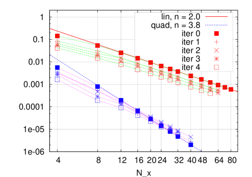
Figure 10: Error in the $l_{2}$-norm for the solutions obtained with linear and and quadratic finite elements with adaptive mesh refinement. The test problem used is that one of section 4.3 with potential $V_{C}$. The straight lines represent the fitted convergence exponents. For linear elements, at each resolution we started with a semi-structured multi-block triangulation and did four AMR iterations. The $l_{2}$ norms of errors for these interations are plotted with the same abscissa, corresponding to the initial resolution. For each resolution, the set of iterations done with quadratic finite elements is the result of $p$-refinement on the linear element meshes.

First of all, no matter how much the mesh is refined, in the end the finite element solution has to be restricted to the same FD grid. What matters for our purposes is the ability of the FD code to properly approximate the solution on this grid, and not at the refined FE mesh. The original FD multi-block grid is already adapted to be sufficiently fine to resolve all important features of the solution.

Second, in the cases here treated both the final solution is a rather regular smooth function, and the domain has regular boundaries. For such cases, standard uniform refinement gives just as good error reduction as AMR. AMR should be advantageous, though, in cases where, for example, the solution has non-smooth features or the domain has non-smooth boundaries.

Finally, the set of grid points where we sample the solution (that is, the multi-block ones) is very special. As already explained, the convergence order at these points is generally higher than one might expect. The special status of these grid points implies local symmetry of the finite element function spaces with respect to these points, which in turn implies superconvergence. AMR can easily break this symmetry and degrade both the error and the convergence order to the level of “ordinary” points. If we wanted to keep this symmetry and have superconvergence, we would have to refine at least within the entire patch, but this would be almost as expensive as refining the entire domain uniformly.

Our experiments do not show particular advantage of using AMR compared to the uniform refinement of semi-structured multi-block triangulations. In our experiments we found that, in general, after a few refinement steps the AMR error saturates, while uniform refinement error continues to decrease. We have found that often, while decreasing the global $l_{2}$ norm, AMR leads to an increase in the $l_{\infty}$ norm of the solution, because the local symmetry is broken at several grid points in the refined mesh.

We have also tried a simple form of $p$-refinement. Namely, using the same set of refined meshes for linear and quadratic elements (see figure 10). We chose several initial multi-block triangulation meshes with different resolutions and did four AMR iterations with linear elements. Then we used the same meshes to increase the order of finite elements to quadratics ($p$-refinement). It turns out that at high resolutions the meshes which give the best error reduction when going from linear to quadratic elements are initial triangulation meshes with no AMR. It happens so because the refined mesh loses the property of local symmetry at some of the grid points, the pointwise superconvergence for quadratic elements is lost and the global $L_{2}$-norm error is observed instead.

5 Brill waves initial data and evolutions

In General Relativity, initial data on a spatial 3D-slice has to satisfy the Hamiltonian and momentum constraint equations [63, 64],

$${}^{3}R-K^{ij}K_{ij}+K^{2} =0$$ (5.1)

$$\nabla_{i}(K^{ij}-g^{ij}K) =0$$ (5.2)

where $K_{ij}$ and $K$ are the extrinsic curvature of the 3D-slice and its trace, respectively, and ${}^{3}R$ the Ricci scalar associated with the spatial metric $g_{ij}$.

Brill waves [65] constitute a simple yet rich example of initial data in numerical relativity. In such a case the extrinsic curvature of the slice is zero, and the above equations reduce to a single one, stating that the Ricci scalar has to vanish:

$${}^{3}R=0\,.$$ (5.3)

If the spatial metric is given up to one unknown function, Eq. (5.3) in principle allows us to solve for such function and thus complete the construction of the initial data. The Brill equation is a special case of (5.3), where the 3-metric is expressed through the conformal transformation $g_{ij}=\psi^{4}\tilde{g}_{ij}$ of an unphysical metric $\tilde{g}_{ij}$, with an unknown conformal factor $\psi$. Equation (5.3) then becomes [66]:

$$(-\nabla_{\tilde{g}}^{2}+\frac{1}{8}\tilde{R})\psi=0$$ (5.4)

where $\tilde{R}$ and $\nabla_{\tilde{g}}^{2}$ are the Ricci scalar curvature and Laplacian of the unphysical metric $\tilde{g}_{ij}$, respectively.

Here we will focus on the axisymmetric case with the unphysical metric given in cylindrical coordinates by

$$\tilde{g}_{ij}=e^{2q(\rho,z)}(d\rho^{2}+dz^{2})+\rho^{2}d\varphi^{2}\,,$$ (5.5)

where $q(\rho,z)$ is a function satisfying the following conditions:

1. regularity at the axis: $q(\rho=0,z)=0$, $\frac{\partial q}{\partial\rho}|_{\rho=0}=0$,

2. asymptotic flatness: $q(\rho,z)|_{r\to\infty}<O(1/r^{2})$, where $r$ is the spherical radius $r~{}=~{}\sqrt{\rho^{2}+z^{2}}$  .

The Hamiltonian constraint equation (5.3) becomes a second order elliptic PDE, which with asymptotically flat boundary conditions at $r\to\infty$ takes the form

$$-\nabla^{2}\psi(\rho,z)+V(\rho,z)\psi(\rho,z) = 0,$$ (5.6)

$$\psi|_{r\to\infty} = 1+\frac{M}{2r}+O(1/r^{2}),$$ (5.7)

with the potential $V(\rho,z)$ given by

$$V=-\frac{1}{4}(q^{\prime\prime}_{\rho\rho}+q^{\prime\prime}_{zz}).$$

We numerically solve this equation using FETK on the 13-patch multi-block spherical domain described in section 4.1 (see figure 7). We use domain parameters $R_{out}~{}=~{}30$, $R_{med}~{}=~{}7$, $a_{c}~{}=~{}1.5$, and grid dimension ratios $N:N_{r,inner}:N_{r,outer}=2:3:12$. Our low-medium-high resolution triple is $N=32$, $N=36$ and $N=40$, except for pointwise convergence tests on the $x$-axis (see figure 13), where we use $N=16$, $N=24$ and $N=36$ (since they all differ by powers of $1.5$).

We impose Robin boundary conditions, as in equation (4.5). The weak form (4.6) and bilinear linearization form (4.7) for this problem are given in section 4.2. Since first order elements lead to unacceptably low convergence orders for most general relativistic applications, from hereon we restrict ourselves to quadratic ones (which should give fourth order convergence if superconvergence is exploited).

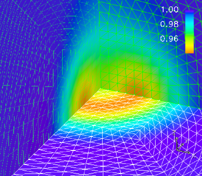
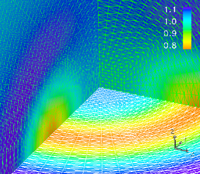
(a)	(b)

Figure 11: Potentials for the two types of Brill waves considered: Holz’ (a) and toroidal (b) forms.

We work with two specific choices for $q(\rho,z)$:

• Holz’ form [67]: $q_{H}(\rho,z)=a_{H}\rho^{2}e^{-r^{2}}$, with amplitude $a_{H}=0.5$;

• toroidal form: $q_{t}(\rho,z)=a_{t}\rho^{2}\exp{\left(-\frac{(\rho-\rho_{0})^{2}}{\sigma_{\rho}^{2}}-\frac{z^{2}}{\sigma_{z}^{2}}\right)}$, with amplitude $a_{t}=0.05$, radius $\rho_{0}=5$, width in $\rho$-direction $\sigma_{\rho}=3.0$ and width in $z$-direction $\sigma_{z}=2.5$.

Holz potential is chosen for historical reasons. It is suitable for evolutions using the cubed sphere system, because initially the wave is concentrated near the origin (at the central patch), and later decays into a sequence of spherical waves. The cubed sphere grid resolves the wave well both at the initial moment, and during the subsequent evolution. For the toroidal potential, the cubed sphere system is adapted even better, since it efficiently removes the dependence on one of the angular coordinates, $\varphi$.

5.1 Importing the initial data into QUILT

Once we have constructed the initial data sets, we analyze and evolve them by importing them into QUILT. For evolutions we use the Generalized Harmonic (GH) first order symmetric hyperbolic formulation of the Einstein’s equations introduced in [68], which features exponential suppression of short-wavelength constraint violations; our multi-block implementation is described in [37].

The set of evolved variables in this system includes the 4-metric $g_{ab}$, its spatial derivatives $\Phi_{iab}=\partial_{i}g_{ab}$ and quantities $\Pi_{ab}=-t^{c}\partial_{c}g_{ab}$, where $t^{c}$ is the unit normal vector to the spatial slice.

To set up the initial data, we first compute the $3+1$ quantities and then convert them to GH variables. The 3-metric $g_{ij}(x,y,z)$ is computed from the conformal factor $\psi(x,y,z)$, in Cartesian coordinates, using the expressions (which follow from 5.5):

$$g_{xx} =\psi^{4}(e^{2q}x^{2}+y^{2})/\rho^{2}, g_{xy} =\psi^{4}(e^{2q}-1)xy/\rho^{2},$$

$$g_{yy} =\psi^{4}(x^{2}+e^{2q}y^{2})/\rho^{2}, g_{zz} =\psi^{4}e^{2q},$$

$$g_{xz} =g_{yz}=0$$

where $\rho=\sqrt{x^{2}+y^{2}}$. Then we construct the rest of the evolved variables, including the gauge source functions $H_{a}=-g^{bc}\Gamma_{a,bc}$ (here $\Gamma_{a,bc}=\frac{1}{2}(\partial_{b}g_{ac}+\partial_{c}g_{ab}-\partial_{a}g_{bc})$ are the Christoffel symbols). The extrinsic curvature is assumed to be zero, $K_{ij}=0$, we also use unit lapse $\alpha=1$, zero shift $\beta_{i}=0$, and zero time derivative of lapse and shift: $\partial_{t}\alpha=\partial_{t}\beta_{i}=0$.

5.2 Convergence of initial data and Hamiltonian constraint

To estimate the quality of our initial data, we evaluate the Hamiltonian constraint violation using the SBP operators, which is in fact equivalent to an independent residual evaluation for the Brill equation (5.6). As is the case with just numerical derivatives, we find that the magnitude and convergence order of the Hamiltonian constraint violation depends on both the order of the SBP operator, and the order of finite elements. In total, computing the Hamiltonian constraint involves two numerical differentiations, therefore it has to converge with the same order as second numerical derivatives. We can see this convergence rate for different SBP operators in figure 12. Table 3 summarizes those results, along with the expected convergence orders for second numerical derivatives.

Consistent with what one expects, for finite difference operators of sufficiently high order the constraints converge with the same order as the finite element solution itself, which should be $3+\sigma$ for some $0<\sigma\leq 1$ (depending on the level of superconvergence obtained). Similarly, below in section 5.3 we will show that the extracted gravitational waves have a similar convergence order.

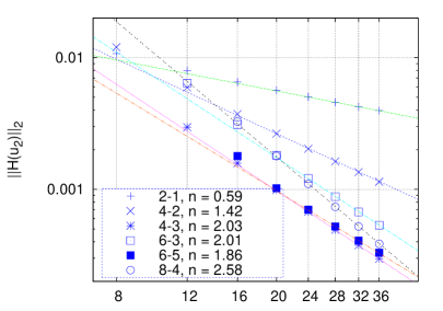
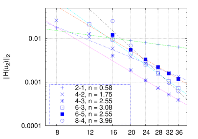
Figure 12: Convergence of the Hamiltonian constraint in the $l_{2}$-norm for Brill waves of Holz (left) and toroidal (right) type, computed using quadratic finite elements and different numerical SBP operators.

$q$	$D_{2-1}$	$D_{4-2}$	$D_{4-3}$	$D_{6-3}$	$D_{6-5}$	$D_{8-4}$
Holz	0.59	1.42	2.03	2.01	1.86	2.58
Toroidal	0.58	1.75	2.55	3.08	2.55	3.96

Table 3: Convergence orders of the Hamiltonian constraint for the two initial data sets in the $l_{2}$-norm.

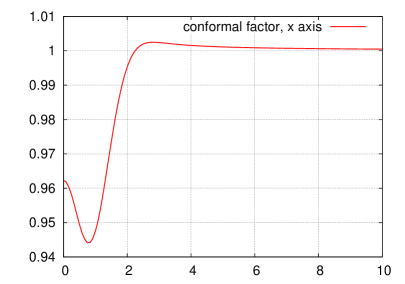
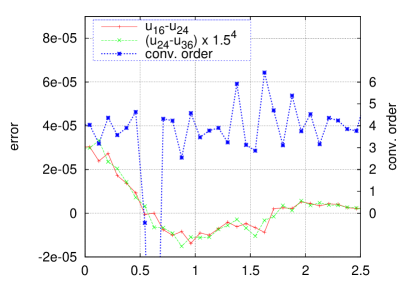
(a)	(b)

Figure 13: (a) 1-d cut through the Brill wave conformal factor $\psi_{fine}$ for problem (a) along the $x$-axis. (b) Errors $\psi_{coarse}-\psi_{medium}$, $\psi_{medium}-\psi_{fine}$, and pointwise convergence order on the 1-d cut along the $x$-axis.

It is not difficult to see why the convergence order is lower for problem (a). This is the order we might expect for quadratic elements on completely unstructured meshes, without superconvergence. The reason that no superconvergence is observed in this case is the following. We have chosen the domain and the width of the Brill wave in such a way that around the boundary of the inner cubical patch the solution varies significantly (see figure 13). Recall that the size of that patch is $a_{c}=1.5$ and the width of the gaussian in the function $q$ is $1$. But this is exactly the place where the local symmetry property is violated most (especially at the corners of the cube), and conditions for superconvergence are the least favorable. Everywhere else the solution varies very slowly and the error is small compared to the error at the boundary of the central cubical patch. With increasing resolution this error dominates in both $l_{2}$ and $l_{\infty}$ norms. The situation is better for the problem with toroidal potential, because most of the variation of the solution is located outside the central cube (recall that the radius of the toroidal wave we use is $r_{0}=5$); though this is still in the inner-patches region (the radius of the spherical boundary between inner and outer patches is $r_{med}=7$).

5.3 Multi-block evolutions

We now demonstrate that our approach for generating initial data on multi-block grids using finite element methods can be successfully used in practice in fully nonlinear relativistic simulations. We do so by presenting results of multi-block evolutions of the Holz set of Brill initial waves constructed above.

In the notation of [68], we fix the damping parameters of the GH formulation to $\gamma_{0}=\gamma_{2}=1$. We used the SBP operator $D_{6-3}$ for spatial differentiations, a 4-th order Runge-Kutta time integrator with adaptive time stepping, and maximally dissipative outer boundary conditions.

The Brill wave amplitude $a_{H}=0.5$ is in the subcritical regime (the critical value is around $a_{cr}\approx 4.85$ [67]). As a result the wave, initially concentrated near the center, dissipates and leaves the domain after a while. Figure 14 shows a convergence plot in time for the Hamiltonian constraint during such evolution. We see that the Hamiltonian constraint converges with a factor of $2-3$ in the $l_{2}$ norm. This has to be one order less convergent than the solution itself, therefore we anticipate the solution to converge with a factor of $3-4$, which is in agreement with the pointwise convergence order of the conformal factor at the initial time (figure 13).

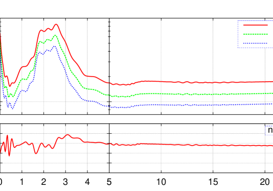
Figure 14: Convergence of the Hamiltonian constraint as a function of time during a multi-block evolution of the Brill wave initial data generated with finite element methods.

We compute gravitational waveforms using a generalized Regge-Wheeler-Zerilli formalism, along the lines of  [37] and extending that reference to the even parity sector (details about that extension will be presented elsewhere). The four-dimensional spacetime metric is decomposed into a spherically symmetric “background” plus a small perturbation [69, 70]. The background part of the metric is identified with the Schwarzschild solution and the radiation content with the difference between the numerically computed solution and the background.

The background metric is written as

$$ds^{2}=\tilde{g}_{\rho\tau}(t,r)dx^{\rho}dx^{\tau}+f^{2}(t,r)\hat{g}_{AB}dx^{A}dx^{B}.$$ (5.8)

with the four-dimensional background manifold split as the product space of a two-dimensional one $\mathcal{M}$ endowed with coordinates $x^{\rho}$ (with $\rho,\tau=0,1$ usually denoting the time and radial coordinate) and a unit 2-sphere $S^{2}$ with coordinates $x^{A}$ (with $A=2,3$ commonly taken as the $\theta$ and $\phi$ polar spherical coordinates). Here $\tilde{g}_{\rho\tau}$ is the metric of the manifold $\mathcal{M}$ and $f^{2}$ is a positive function of $x^{\rho}$. If using the areal radius as a coordinate we have $f=r$. The metric of the 2-sphere is taken to be $\hat{g}_{AB}=\textrm{diag}(1,\sin^{2}\theta)$ in polar spherical coordinates.

The metric perturbation is decomposed in terms of scalar, vector and tensor spherical harmonics [71, 72, 37]. The decomposition naturally splits the different $(\ell,m)$ modes into even $(-1)^{\ell}$ and odd $(-1)^{\ell+1}$ parity under reflections about the origin. The two different parities are handled separately. Odd and even-parity perturbations are described by the Regge-Wheeler [69] and Zerilli [70] functions, respectively.

The dominant modes in the evolutions of the Brill data constructed above are the $\ell=2,4$ even parity, axisymmetric ones (see figure 15). Figures 16 and 17 display the corresponding Zerilli functions and their convergence behavior, extracted at a radius $r_{e}=12.75$. The observed convergence factors for the $\ell=2$ and $\ell=4$ modes are around four and three, respectively, which are consistent with the convergence factors from quadratic elements with superconvergence for the initial data and the $D_{6-3}$ SBP operator and fourth-order Runge-Kutta for the evolution.

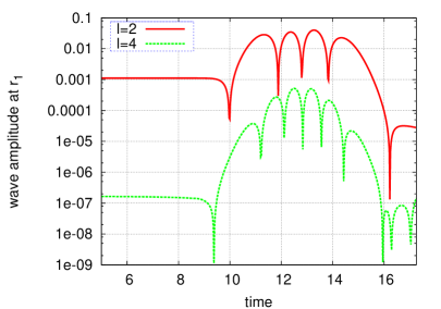
Figure 15: Nonzero components of gravitational radiation $\ell=2$ and $\ell=4$, $m=0$, extracted at radius $r_{e}=12.75$.

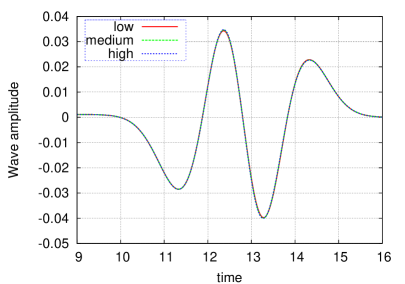
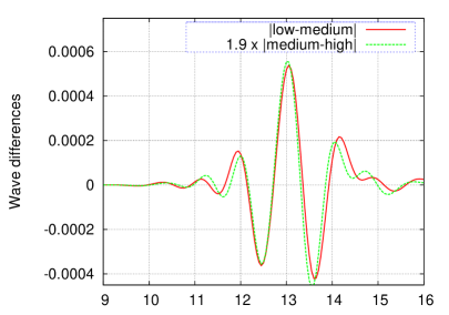
(a)	(b)

Figure 16: Zerilli function (left) and self-differences (right) for the $(\ell=2,m=0)$ mode, scaled according to fourth order convergence.

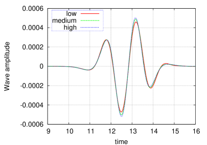
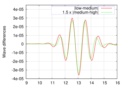
(a)	(b)

Figure 17: Zerilli function (left) and self-differences (right) for the $(\ell=4,m=0)$ mode, scaled according to third order convergence.

Final remarks

In this paper we followed a finite element approach for generating initial data satisfying the Einstein constraint equations on semi-structured, multi-block three-dimensional domains. In section 4 we used semi-structured multi-block triangulations to solve for some test problems with known closed-form solutions. The obtained linear and quadratic finite element solutions were then restricted to the multi-block grid, and their convergence, as well as the convergence of their first and second derivatives, was evaluated numerically using independent high-order finite difference operators satisfying summation by parts (SBP). While the linear elements solution showed usual 2-nd order convergence (unacceptably low for many relativistic applications), for quadratic elements we obtained superconvergence with order $3+\sigma$ (with $0<\sigma\leq 1$) on the grid, due to the approximate local symmetry at the mesh vertices with respect to the local inversion of the multi-block triangulations.

Initial data for a first-order formulation of the Einstein equations involves first derivatives of the solution of the constraints equation. Computing the constraints or right-hand sides of the evolution equations requires taking derivatives twice. In subsection 4.4 we analyzed convergence of the first and second numerical derivatives, taken with different high-order SBP operators. For quadratic elements, the first numerical derivative was observed to converge with either the superconvergence order $3+\sigma$, or the order of SBP operator. The latter is a transient error behavior and happens when the FE error is still smaller than the error of numerical differentiation.

In subsection 4.5 we discussed three factors which make adaptive mesh refinement (AMR) unnecessary and/or less efficient for the problems here considered when compared to global refinement: the fact that the multi-block grid is already tailored to resolve fine features of the solution, the need to restrict the finite element solution to the same grid, and the superconvergence properties of the quadratic elements solution. Because we lose superconvergence when using completely unstructured meshes, adaptively refining the solution sometimes makes the errors larger (see figure 10 for an example). However, we also noted that AMR would likely become advantageous for other problems with more singular solution features.

Finally, in section 5 we presented numerical experiments with Brill waves. The constraint equations in this case reduce to a single elliptic one (5.6) on the conformal factor $\psi$, which has to be differentiated once to obtain the full set of initial data variables in the generalized harmonic formulation (subsection 5.1). Subsection 5.2 presented a convergence analysis of the initial data and Hamiltonian constraint, and confirmed that the initial data computed with quadratic finite elements shows the desired order of convergence $>3$ (see table 3). Finally, in section 5.3 we demonstrated stable, $>3$-rd order convergent multi-block evolutions of subcritical Brill waves with finite differences, summation by parts operators, and extracted the first two dominant radiation modes from the numerical solution.

This paper shows that generating initial data on semi-structured multi-block triangulations using finite element methods is a feasible approach which works well in practice. Future work might include adding higher order and/or spectral elements to this approach.

References

- [1] L. Lehner, Numerical relativity: A review, Class. Quantum Grav. 18 (2001) R25–R86.
- [2] F. Pretorius, Evolution of binary black hole spacetimes, Phys. Rev. Lett. 95 (2005) 121101.
- [3] S. Bonazzola, J. Frieben, E. Gourgoulhon, J.-A. Marck, Spectral methods in general relativity – v toward the simulation of 3D-gravitational collapse of neutron stars, in: Proceedings of the Third International Conference on Spectral and High Order Methods, Houston Journal of Mathematics (1996), University of Houston, 1996.
-
[4]
J. N. Philippe Grandclément, Spectral methods for numerical relativity,
Living Reviews in Relativity 12 (1).
URL http://www.livingreviews.org/lrr-2009-1 - [5] H. P. Pfeiffer, L. E. Kidder, M. A. Scheel, S. A. Teukolsky, A multidomain spectral method for solving elliptic equations, Comput. Phys. Commun. 152 (2003) 253–273.
-
[6]
G. B. Cook, Initial data for numerical relativity, Living Rev. Relativity 3
(2000) 5.
URL http://www.livingreviews.org/lrr-2000-5 - [7] H. P. Pfeiffer, S. A. Teukolsky, G. B. Cook, Quasi-circular orbits for spinning binary black holes, Phys. Rev. D 62 (2000) 104018.
- [8] L. E. Kidder, L. S. Finn, Spectral methods for numerical relativity. the initial data problem, Phys. Rev. D 62 (2000) 084026.
- [9] H. Pfeiffer, Initial data for black hole evolutions, Ph.D. thesis, Cornell University, Ithaca, New York State (2003).
- [10] S. Bonazzola, E. Gourgoulhon, J.-A. Marck, Numerical approach for high precision 3-D relativistic star models, Phys. Rev. D. 58 (1998) 104020.
- [11] L.-M. Lin, J. Novak, A new spectral apparent horizon finder for 3D numerical relativity, Class. Quant. Grav. 24 (2007) 2665–2676.
- [12] T. Nakamura, Y. Kojima, K. Oohara, A method of determining apparent horizons in three-dimensional numerical relativity, Phys. Lett. A 106 (5-6) (1984) 235–238.
-
[13]
E. Tadmor, Spectral methods for hyperbolic problems, in: Lecture notes
delivered at Ecole des Ondes, ”Méthodes numériques d’ordre
élevé pour les ondes en régime transitoire”, INRIA–Rocquencourt
January 24-28., 1994.
URL http://www.cscamm.umd.edu/people/faculty/tadmor/pub/spectral-approximations/Tadmor.INRIA-94.pdf - [14] M. A. Scheel, et al., High-accuracy waveforms for binary black hole inspiral, merger, and ringdown, Phys. Rev. D79 (2009) 024003.
- [15] L. E. Kidder, M. A. Scheel, S. A. Teukolsky, E. D. Carlson, G. B. Cook, Black hole evolution by spectral methods, Phys. Rev. D 62 (2000) 084032.
- [16] L. Kidder, M. Scheel, S. Teukolsky, G. Cook, Spectral evolution of Einstein’s equations, in: Miniprogram on Colliding Black Holes: Mathematical Issues in Numerical Relativity, Institute for Theoretical Physics, UCSB, Santa Barbara, CA, 2000.
- [17] M. A. Scheel, L. E. Kidder, L. Lindblom, H. P. Pfeiffer, S. A. Teukolsky, Toward stable 3d numerical evolutions of black-hole spacetimes, Phys. Rev. D 66 (2002) 124005.
- [18] M. A. Scheel, H. P. Pfeiffer, L. Lindblom, L. E. Kidder, O. Rinne, S. A. Teukolsky, Solving Einstein’s equations with dual coordinate frames, Phys. Rev. D 74 (2006) 104006.
- [19] R. M. Wald, General relativity, The University of Chicago Press, Chicago, 1984.
-
[20]
B. Zink, E. Schnetter, M. Tiglio, Multi-patch methods in general relativistic
astrophysics - i. hydrodynamical flows on fixed backgrounds (2007).
URL http://www.citebase.org/abstract?id=oai:arXiv.org:0712.%%****␣fetkbw.bbl␣Line␣100␣****0353 -
[21]
J. A. Font, Numerical hydrodynamics in general relativity, Living Reviews in
Relativity 6 (4).
URL http://www.livingreviews.org/lrr-2003-4 -
[22]
J. M. Martí, E. Müller, Numerical hydrodynamics in special
relativity, Living Rev. Relativity 2 (1999) 3.
URL http://www.livingreviews.org/lrr-1999-3 -
[23]
M. D. Duez, L. E. Kidder, S. A. Teukolsky, Evolving relativistic fluid
spacetimes using pseudospectral methods and finite differencing (2007).
URL http://www.citebase.org/abstract?id=oai:arXiv.org:gr-qc%/0702126 - [24] J. Isenberg, Constant mean curvature solution of the Einstein constraint equations on closed manifold, Class. Quantum Grav. 12 (1995) 2249–2274.
- [25] J. Isenberg, V. Moncrief, A set of nonconstant mean curvature solution of the Einstein constraint equations on closed manifolds, Class. Quantum Grav. 13 (1996) 1819–1847.
- [26] M. Holst, J. Kommemi, G. Nagy, Rough solutions of the Einstein constraint equations with nonconstant mean curvature, submitted to Comm. Math. Phys. Available as arXiv:0708.3410v2 [gr-qc].
- [27] M. Holst, G. Nagy, G. Tsogtgerel, Rough solutions of the Einstein constraints on closed manifolds without near-CMC conditions, submitted for publication. Available as arXiv:0712.0798v1 [gr-qc].
- [28] M. Holst, G. Nagy, G. Tsogtgerel, Far-from-constant mean curvature solutions of Einstein’s constraint equations with positive Yamabe metrics, submitted to Phys. Rev. Lett.
-
[29]
M. Holst, Adaptive numerical treatment of elliptic systems on manifolds,
Advances in Computational Mathematics 15 (2001) 139–191.
URL citeseer.ist.psu.edu/holst01adaptive.html - [30] M. Holst, G. Tsogtgerel, Adaptive finite element approximation of nonlinear geometric PDE, preprint.
- [31] M. Holst, G. Tsogtgerel, Convergent adaptive finite element approximation of the Einstein constraints, preprint.
- [32] L. Wahlbin, Superconvergence in Galerkin Finite Element Methods, Springer-Verlag New York, 1995.
- [33] E. Schnetter, P. Diener, E. N. Dorband, M. Tiglio, A multi-block infrastructure for three-dimensional time- dependent numerical relativity, Class. Quant. Grav. 23 (2006) S553–S578.
-
[34]
L. Lehner, O. Reula, M. Tiglio, Multi-block simulations in general relativity:
high order discretizations, numerical stability, and applications, Classical
and Quantum Gravity 22 (2005) 5283.
URL http://www.citebase.org/abstract?id=oai:arXiv.org:gr-qc%/0507004 -
[35]
P. Diener, E. N. Dorband, E. Schnetter, M. Tiglio, New, efficient, and accurate
high order derivative and dissipation operators satisfying summation by
parts, and applications in three-dimensional multi-block evolutions, Journal
of Scientific Computing 32 (2007) 109.
URL doi:10.1007/s10915-006-9123-7 - [36] E. N. Dorband, E. Berti, P. Diener, E. Schnetter, M. Tiglio, A numerical study of the quasinormal mode excitation of Kerr black holes, Phys. Rev. D 74 (2006) 084028.
- [37] E. Pazos, et al., How far away is far enough for extracting numerical waveforms, and how much do they depend on the extraction method?, Class. Quant. Grav. 24 (2007) S341–S368.
- [38] R. Bank, M. Holst, A new paradigm for parallel adaptive mesh refinement, SIAM Rev. 45 (2) (2003) 291–323.
- [39] M. Holst, The finite element toolkit (FeTK), Website, http://www.fetk.org.
- [40] B. Aksoylu, D. Bernstein, S. D. Bond, M. Holst, Generating initial data in general relativity using adaptive finite element methods, Tech. rep., LSU Center for Computation and Technology (CCT) Technical Report 08-09 (2008).
- [41] B. Aksoylu, M. Holst, Optimality of multilevel preconditioners for local mesh refinement in three dimensions, SIAM J. Numer. Anal. 44 (3) (2006) 1005–1025.
- [42] B. Aksoylu, S. Bond, M. Holst, An odyssey into local refinement and multilevel preconditioning III: Implementation and numerical experiments, SIAM J. Sci. Comput. 25 (2) (2003) 478–498.
- [43] L. Chen, M. Holst, J. Xu, Convergence and optimality of adaptive mixed finite element methods, submitted to Math. Comp.
- [44] L. Chen, M. Holst, J. Xu, The finite element approximation of the nonlinear Poisson-Boltzmann Equation, SIAM J. Numer. Anal. 45 (6) (2007) 2298–2320.
- [45] R. A. Adams, Sobolev Spaces, Academic Press, Inc., 1987.
- [46] M. S. Gockenbach, Understanding and Implementing the Finite Element Method, SIAM, 2006.
- [47] P.-L. George, H. Borouchaki, Delauney Triangulation and Meshing: Application to Finite Elements, Kogan Page, 1998.
- [48] C.-M. Chen, Superconvergence of Finite Element Solutions and Their Derivatives, Hunan Science Press, 1982, (in Chinese).
- [49] Q.-D. Zhu, Q. Lin, Hyperconvergence Theory of Finite Elements, Hunan Science and Technology Publishing House, Changsha, P.R. China, 1989, (in Chinese).
- [50] M. Křížek, P. Neittaanmäki, On a global superconvergence of the gradient of linear triangular elements, J. Comput. Appl. Math. 18 (2) (1987) 221–233.
-
[51]
A. H. Schatz, I. H. Sloan, L. B. Wahlbin, Superconvergence in finite element
methods and meshes that are locally symmetric with respect to a point, SIAM
Journal on Numerical Analysis 33 (2) (1996) 505–521.
URL http://link.aip.org/link/?SNA/33/505/1 - [52] A. H. Schatz, Pointwise error estimates, superconvergence and extrapolation (1998) 237–247.
- [53] J. F. Sallee, The middle-cut triangulations of the -cube 5 (3) (1984) 407–419.
- [54] H. W. Kuhn, Some combinatorial lemmas in topology, IBM Journal of Research and Development 4 (1960) 508–524.
- [55] C. Min, Simplicial isosurfacing in arbitrary dimension and codimension, Journal of Computational Physics 190 (1) (2003) 295–310.
- [56] D. Braess, Finite Elements: Theory, Fast Solvers, and Applications in Solid Mechanics, Cambridge University Press, 2007.
- [57] S. Brenner, L. Scott, The Mathematical Theory of Finite Element Methods, Springer – Verlag, 2003.
- [58] A. Ern, J. Guermond, Theory and practice of finite elements, Springer, 2004.
- [59] B. Gustafsson, On the implementation of boundary conditions for the method of lines, BIT Numerical Mathematics 38 (2) (1998) 293–314.
- [60] N. D. Levine, Superconvergent recovery of the gradient from piecewise linear finite element approximations, IMA Journal of Numerical Analysis 5 (1985) 407–427.
- [61] G. Goodsell, J. Whiteman, A unified treatment of superconvergent recovered gradient functions for piecewise linear finite element approximations, International Journal of Numerical Methods in Engineering 27 (1989) 469–481.
- [62] Q. L. H. Blum, R. Rannacher, Asymptotic error expansion and richardson extrapolation for linear finite elements, Numer. Math. 49 (1986) 11–37.
- [63] R. Arnowitt, S. Deser, C. W. Misner, The dynamics of general relativity, in: L. Witten (Ed.), Gravitation: An introduction to current research, John Wiley, New York, 1962, pp. 227–265.
- [64] C. W. Misner, K. S. Thorne, J. A. Wheeler, Gravitation, W. H. Freeman, San Francisco, 1973.
- [65] D. R. Brill, On the positive definite mass of the bondi-weber-wheeler time-symmetric gravitational waves, Ann. Phys. 7 (1959) 466–483.
- [66] N. Ó Murchadha, Brill Waves, in: B. L. Hu, T. A. Jacobson (Eds.), Directions in General Relativity: Papers in Honor of Dieter Brill, Volume 2, 1993, pp. 210–+.
-
[67]
M. Alcubierre, G. Allen, B. Bruegmann, G. Lanfermann, E. Seidel, W.-M. Suen,
M. Tobias, Gravitational collapse of gravitational waves in 3d numerical
relativity, Physical Review D 61 (2000) 041501.
URL http://www.citebase.org/abstract?id=oai:arXiv.org:gr-qc%/9904013 - [68] L. Lindblom, M. A. Scheel, L. E. Kidder, R. Owen, O. Rinne, A new generalized harmonic evolution system, Classical and Quantum Gravity 23 (2006) 447–+.
- [69] T. Regge, J. Wheeler, Stability of a Schwarzschild singularity, Phys. Rev. 108 (4) (1957) 1063–1069.
- [70] F. J. Zerilli, Effective potential for even-parity Regge-Wheeler gravitational perturbation equations, Phys. Rev. Lett. 24 (13) (1970) 737–738.
- [71] F. J. Zerilli, Tensor harmonics in canonical form for gravitational radiation and other applications, J. Math. Phys. 11 (1970) 2203–2208.
- [72] K. Thorne, Multipole expansions of gravitational radiation, Rev. Mod. Phys. 52 (2) (1980) 299.
- [73] T. Goodale, G. Allen, G. Lanfermann, J. Massó, T. Radke, E. Seidel, J. Shalf, The Cactus framework and toolkit: Design and applications, in: Vector and Parallel Processing – VECPAR’2002, 5th International Conference, Lecture Notes in Computer Science, Springer, Berlin, 2003.
-
[74]
Cactus Computational Toolkit home page.
URL http://www.cactuscode.org/ - [75] E. Schnetter, S. H. Hawley, I. Hawke, Evolutions in 3D numerical relativity using fixed mesh refinement, Class. Quantum Grav. 21 (6) (2004) 1465–1488.
-
[76]
Mesh Refinement with Carpet.
URL http://www.carpetcode.org/ - [77] E. Anderson, Z. Bai, C. Bischof, S. Blackford, J. Demmel, J. Dongarra, J. Du Croz, A. Greenbaum, S. Hammarling, A. McKenney, D. Sorensen, LAPACK Users’ Guide, 3rd Edition, Society for Industrial and Applied Mathematics, Philadelphia, PA, 1999.
-
[78]
LAPACK: Linear Algebra Package.
URL http://www.netlib.org/lapack/ -
[79]
BLAS: Basic Linear Algebra Subroutines.
URL http://www.netlib.org/blas/ -
[80]
Netlib Repository.
URL http://www.netlib.org/ -
[81]
G. Burns, R. Daoud, J. Vaigl, LAM: An Open Cluster Environment for
MPI, in: Proceedings of Supercomputing Symposium, 1994, pp. 379–386.
URL http://www.lam-mpi.org/download/files/lam-papers.tar.gz - [82] J. M. Squyres, A. Lumsdaine, A Component Architecture for LAM/MPI, in: Proceedings, 10th European PVM/MPI Users’ Group Meeting, No. 2840 in Lecture Notes in Computer Science, Springer-Verlag, Venice, Italy, 2003, pp. 379–387.
-
[83]
LAM: LAM/MPI Parallel Computing.
URL http://www.lam-mpi.org/ - [84] W. Gropp, E. Lusk, N. Doss, A. Skjellum, A high-performance, portable implementation of the MPI message passing interface standard, Parallel Computing 22 (6) (1996) 789–828.
- [85] W. D. Gropp, E. Lusk, User’s Guide for mpich, a Portable Implementation of MPI, Mathematics and Computer Science Division, Argonne National Laboratory, ANL-96/6 (1996).
-
[86]
MPICH: ANL/MSU MPI implementation.
URL http://www-unix.mcs.anl.gov/mpi/mpich/ -
[87]
MPI: Message Passing Interface Forum.
URL http://www.mpi-forum.org/