The Stochastic Dynamics of Rectangular and V-shaped Atomic Force Microscope Cantilevers in a Viscous Fluid and Near a Solid Boundary

Abstract

Using a thermodynamic approach based upon the fluctuation-dissipation theorem we quantify the stochastic dynamics of rectangular and V-shaped microscale cantilevers immersed in a viscous fluid. We show that the stochastic cantilever dynamics as measured by the displacement of the cantilever tip or by the angle of the cantilever tip are different. We trace this difference to contributions from the higher modes of the cantilever. We find that contributions from the higher modes are significant in the dynamics of the cantilever tip-angle. For the V-shaped cantilever the resulting flow field is three-dimensional and complex in contrast to what is found for a long and slender rectangular cantilever. Despite this complexity the stochastic dynamics can be predicted using a two-dimensional model with an appropriately chosen length scale. We also quantify the increased fluid dissipation that results as a V-shaped cantilever is brought near a solid planar boundary.

I Introduction

The stochastic dynamics of micron and nanoscale cantilevers immersed in a viscous fluid are of broad scientific and technological interest Butt and Jaschke (1995); Ekinci and Roukes (2005). Of particular importance is the oscillating cantilever that is central to atomic force microscopy Binnig et al. (1986); Garcia and Perez (2002). Significant theoretical progress has been made using simplified models in the limit of long and thin rectangular cantilevers Tuck (1969); Sader (1998); Clarke et al. (2005). In this case, a two-dimensional approximation is appropriate (therefore neglecting effects due to the tip of the cantilever) and has yielded important insights. However, it is not certain how well these approximations work for many situations of direct experimental interest. For example, a commonly used cantilever in atomic force microscopy is V-shaped and a theoretical description of the dynamics of these cantilevers in fluid is not available.

Furthermore, micron and nanoscale cantilevers are often used in close proximity to a solid boundary either by necessity or out of experimental interest. It is well known experimentally and theoretically that the presence of a solid boundary increases the fluid dissipation resulting in reduced quality factors and reduced resonant frequencies Benmouna and Johannsmann (2002); Nnebe and Schneider (2004); Clarke et al. (2005, 2006a, 2006b); Green and Sader (2005a, b); Harrison et al. (2007). Again, theoretical descriptions are available in the limit of long and thin rectangular cantilevers and it is uncertain if these approaches can be applied to these more complex geometries.

In this paper we use a powerful thermodynamic approach to quantify the stochastic dynamics of cantilevers due to Brownian motion for experimentally relevant geometries for the precise conditions of experiment including the presence of a planar boundary. Our results are valid for the precise three-dimensional geometry of interest and include a complete description of the fluid-solid interactions. Using these results we are able to compare with available theory to yield further physical insights and to suggest simplified analytical approaches to describe the cantilever dynamics for these complex situations.

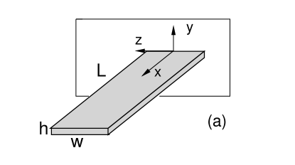
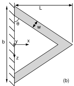
Figure 1: Schematics of the two micron scale cantilever geometries considered (not drawn to scale). Panel (a), A rectangular cantilever with aspect ratios $L/h=98.5$, $w/h=14.5$, and $L/w=6.8$. The cantilever is composed of silicon with density $\rho_{c}=$ 2329 kg/$\text{m}^{3}$ and Youngs Modulus $E=$ 174 GPa. Panel (b), A V-shaped cantilever with aspect ratios $L/h=233$, $w/h=30$, and $L/w=7.8$. The total width between the two arms normalized by the width of a single arm is $b/w=10.36$. The cantilever planform is an equilateral triangle with $\theta=\pi/3$. The cantilever is composed of silicon nitride with $\rho_{c}=3100$kg/$\text{m}^{3}$ and $E=172$GPa. The specific dimensions for the rectangular and V-shaped cantilever are given in Table 1.

II Thermodynamic Approach – Fluctuations from Dissipation

The stochastic dynamics of micron and nanoscale cantilevers driven by thermal or Brownian motion can be quantified using strictly deterministic calculations. This is accomplished using the fluctuation-dissipation theorem since the cantilever remains near thermodynamic equilibrium Paul and Cross (2004); Paul et al. (2006). We briefly review this approach for the case of determining the stochastic displacement of the cantilever tip and then extend it to the experimentally important case of determining the stochastic dynamics of the angle of the cantilever tip.

The autocorrelation of equilibrium fluctuations in cantilever displacement can be determined from the deterministic response of the cantilever to the removal of a step force from the tip of the cantilever (i.e. a transverse point force removed from the distal end of the cantilever). If this force $f(t)$ is given by

$$f(t)=\left\{\begin{array}[c]{cc}F_{0}&\text{for }t<0\\ 0&\text{for }t\geq 0,\end{array}\right.$$ (1)

where $t$ is time and $F_{0}$ is the magnitude of the force, then the autocorrelation of the equilibrium fluctuations in the displacement of the cantilever tip is given directly by

$$\left<u_{1}(0)u_{1}(t)\right>=k_{B}T\frac{U_{1}(t)}{F_{0}},$$ (2)

where $k_{B}$ is Boltzmann’s constant, $T$ is the temperature, and $\left<\right>$ is an equilibrium ensemble average. In our notation lower case letters represent stochastic variables ($u_{1}(t)$ is the stochastic displacement of the cantilever tip) and upper case letters represent deterministic variables ($U_{1}(t)$ represents the deterministic ring down of the cantilever tip due to the step force removal). The spectral properties of the stochastic dynamics are given by the Fourier transform of the autocorrelation.

The thermodynamic approach is valid for any conjugate pair of variables Paul and Cross (2004). For example, it is common in experiment to use optical techniques to measure the angle of the cantilever tip as a function of time Garcia and Perez (2002). It has also been proposed to use piezoresistive techniques to measure voltage as a function of time Arlett et al. (2006). The thermodynamic approach remains valid for these situations by choosing the correct conjugate pair of variables.

In this paper we also explore the stochastic dynamics of the angle of the cantilever tip. In this case, the angle of the cantilever tip is conjugate to a step point-torque applied to the cantilever tip. If this torque is given by

$$\tau(t)=\left\{\begin{array}[c]{cc}\tau_{0}&\text{for }t<0\\ 0&\text{for }t\geq 0,\end{array}\right.$$ (3)

where $\tau_{0}$ is the magnitude of the step torque, then the autocorrelation of equilibrium fluctuations in cantilever tip-angle $\theta(t)$ is given by

$$\left<\theta_{1}(0)\theta_{1}(t)\right>=k_{B}T\frac{\Theta_{1}(t)}{\tau_{0}}.$$ (4)

Here $\Theta_{1}(t)$ represents the deterministic ring down, as measured by the tip-angle, resulting from the removal of a step point-torque. Again, the Fourier transform of the autocorrelation yields the noise spectrum.

	$L(\mu$m)	$w(\mu$m)	$h(\mu$m)	$k$ (N/m)	$k_{t}$ (N-m/rad)	$f_{0}$ (kHz)
(1)	197	29	2	1.3	$1.6\times 10^{-8}$	71
(2)	140	15.6	0.6	0.1	$8.9\times 10^{-10}$	38

Table 1: Summary of the cantilever geometries and material properties. (1) The rectangular cantilever. (2) The V-shaped cantilever used is the commercially available Veeco MLCT Type E microlever that is used in AFM vee . The geometry is given by the cantilever length $L$, width $w$, and height $h$. For the V-shaped cantilever the total length between the two arms at the base is $b=161.64\mu$m. The cantilever spring constant $k$, torsional spring constant $k_{t}$, and resonant frequency in vacuum $f_{0}$ are determined using finite element numerical simulations. The cantilevers are immersed in water with density $\rho_{l}$ = 997 kg/$\text{m}^{3}$ and dynamic viscosity $\eta$ = 8.59 $\times$ $10^{-4}$ kg/m-s.

A powerful aspect of this approach is that it is possible to use deterministic numerical simulations to determine $U_{1}(t)$ and $\Theta_{1}(t)$ for the precise cantilever geometries and conditions of experiment. This includes the full three-dimensionality of the dynamics which are not accounted for in available theoretical descriptions. The numerical results can be used to guide the development of more accurate theoretical models.

III The stochastic dynamics of cantilever tip-deflection and tip-angle

The stochastic dynamics of the cantilever tip-displacement $u_{1}(t)$ and that of the tip-angle $\theta_{1}(t)$ yield interesting differences. Using the thermodynamic approach, insight into these differences can be gained by performing a mode expansion of the cantilever using the initial deflection required by the deterministic calculation. The two cases of a tip-force and a tip-torque result in a significant difference in the mode expansion coefficients which can be directly related to the resulting stochastic dynamics.

For small deflections the dynamics of a cantilever with a non-varying cross section are given by the Euler-Bernoulli beam equation,

$$\mu\frac{\partial^{2}U}{\partial t^{2}}+EI\frac{\partial^{4}U}{\partial x^{4}}=0,$$ (5)

where $U(x,t)$ is the transverse beam deflection, $\mu$ is the mass per unit length, $E$ is Young’s modulus, and $I$ is the moment of inertia Landau and Lifshitz (1959). For the case of a cantilever where a step force has been applied to the tip at some time in the distant past the steady deflection of the cantilever at $t=0$ is given by

$$U(x)=-\frac{F_{0}}{2EI}\left(\frac{x^{3}}{3}-Lx^{2}\right),$$ (6)

where $L$ is the length of the cantilever and the appropriate boundary conditions are $U(0)=U^{\prime}(0)=U^{\prime\prime}(L)=0$ and $U^{\prime\prime\prime}(L)=-F_{0}/EI$. The prime denotes differentiation with respect to $x$.

Similarly, the deflection of the same cantilever beam due to the application of a point-torque at the cantilever-tip is quadratic in axial distance and is given by

$$U(x)=\frac{\tau_{0}}{2EI}x^{2},$$ (7)

where the appropriate boundary conditions are $U(0)=U^{\prime}(0)=U^{\prime\prime\prime}(L)=0$ and $U^{\prime\prime}(L)=\tau_{0}/EI$. The angle of the cantilever measured relative to the horizontal or undisplaced cantilever is then given by $\tan\Theta=U^{\prime}(x)$.

The mode shapes for a cantilevered beam are given by

$$\Phi_{n}(x) = -\left(\cos\kappa L+\cosh\kappa L\right)\left(\cos\kappa x-\cosh\kappa x\right)$$ (8)

$$- \left(\sin\kappa L-\sinh\kappa L\right)\left(\sin\kappa x-\sinh\kappa x\right),$$

where $n$ is the mode number, and the characteristic frequencies are given by $\kappa^{4}=\omega^{2}\mu/EI$. The mode numbers $\kappa$ are solutions to $1+\cos{\kappa L}\cosh{\kappa L}=0$ Landau and Lifshitz (1959). The initial cantilever displacement given by Eqs. (6) and (7) can be expanded into the beam modes

$$U(x)=\displaystyle\sum_{n=1}^{\infty}a_{n}\Phi_{n}(x),$$ (9)

with mode coefficients $a_{n}$. The total energy $E_{b}$ of the deflected beam is given by

$$E_{b}=\frac{EI}{2}\int_{0}^{L}U^{\prime\prime}(x)^{2}dx,$$ (10)

which is entirely composed of bending energy. The fraction of the total bending energy contained in an individual mode is given by

$$b_{n}=\frac{EI}{2E_{b}}\int_{0}^{L}\left(a_{n}\Phi_{n}^{\prime\prime}(x)\right)^{2}dx.$$ (11)

The coefficients $b_{n}$ for the rectangular cantilever of Table 1 are shown in Table 2. For the case of a force applied to the cantilever tip, 97% of the total bending energy is contained in the fundamental mode and the energy contained in the higher modes decays rapidly with less than 1% of the energy contained in mode three. When a point-torque is applied to the same beam it is clear that a significant portion of the bending energy is spread over the higher modes. Only 61% of the energy is contained in the fundamental mode and the decay in energy with mode number is more gradual. The fifth mode for the tip-torque case contains more energy than the second mode for the tip-force case. Although we have only discussed a mode expansion for the rectangular cantilever, the V-shaped cantilever will exhibit similar trends since the transverse mode shapes are similar to that of a rectangular beam Stark et al. (2001).

The variation in the energy distribution among the modes required to describe the initial deflection of the cantilever can be immediately connected to the resulting stochastic dynamics. For the deterministic calculations the initial displacement can be arbitrarily set to a small value. In this limit the modes of the cantilever beam are not coupled through the fluid dynamics. As a result, the stochastic dynamics of each mode can be treated as the ring down of that mode from the initial deflection. This indicates that the more energy that is distributed amongst the higher modes initially the more significant the ring down and, using the fluctuation-dissipation theorem, the more significant the stochastic dynamics.

The mode expansion clearly shows that the tip-torque case has more energy in the higher modes. This suggests that stochastic measurements of the cantilever tip-angle will have a stronger signature from the higher modes than measurements of cantilever tip-displacements. Using finite element simulations for the precise geometries of interest we quantitatively explore these predictions.

$n$	$b_{n}$ (tip-force)	$b_{n}$ (tip-torque)
$1$	0.97068	0.61308
$2$	0.02472	0.18830
$3$	0.00315	0.06473
$4$	0.00082	0.03309
$5$	0.00030	0.02669

Table 2: The fraction of the total energy $E_{b}$ contained in the first five beam modes given by the coefficients $b_{n}$. The tip-force results are for a rectangular beam that has been deflected by the application of a point force to the cantilever tip. The tip-torque results are for a rectangular beam that has been deflected by the application of a point torque to the cantilever tip. The coefficients clearly show that the tip-torque case has significantly more energy contained in the higher modes.

	$\left<u_{1}^{2}\right>^{1/2}$(nm)	$\left<\theta_{1}^{2}\right>^{1/2}$(rad)
(1)	$5.6$	$5.0\times 10^{-7}$
(2)	$20$	$7.0\times 10^{-9}$

Table 3: The magnitude of stochastic fluctuations in tip-deflection and in tip-angle for the rectangular (1) and V-shaped (2) cantilevers. These values were obtained from numerical simulations simulations of the beams in vacuum.

IV The stochastic dynamics of a rectangular cantilever

We have performed deterministic numerical simulations of the three-dimensional, time dependent, fluid-solid interaction problem to quantify the stochastic dynamics of a rectangular cantilever immersed in water using the thermodynamic approach discussed in Section II. The deterministic numerical simulations are done using a finite element approach that is described elsewhere Yang and Makhijani (1994); ESI .

The stochastic fluctuations in cantilever tip-displacement for a rectangular cantilever in water have been described elsewhere  Chon et al. (2000); Paul and Cross (2004); Paul et al. (2006); Clark and Paul (2006). In the following we compare these results with the stochastic dynamics as determined by the fluctuations of the cantilever tip-angle. The geometry of the the specific micron scale cantilever we explore is given in Table 1.

As discussed in Section II the autocorrelations in equilibrium fluctuations follow immediately from the ring down of the cantilever due to the removal of a step force (to yield $\left<u_{1}(0)u_{1}(t)\right>$) or step point-torque (to yield $\left<\theta_{1}(0)\theta_{1}(t)\right>$). The autocorrelations of the rectangular cantilever are shown in Fig. 2. The magnitude of the noise is quantified by the root mean squared tip-angle and deflection which is listed in Table 3.

A comparison of the autocorrelations yields some interesting features. At short times $\left<\theta_{1}(0)\theta_{1}(t)\right>$ shows the presence of higher harmonic contributions. This is shown more clearly in the inset of Fig. 2. This further suggests that the angle autocorrelations are more sensitive to higher mode dynamics as discussed in Section III.

Figure 2: The normalized autocorrelation of the rectangular cantilever for tip-deflection (solid) and tip-angle (dashed). (Inset) A detailed view of the autocorrelation at short time differences to illustrate the influence of higher modes in the tip-angle measurements.

The Fourier transform of the autocorrelations yield the noise spectra shown in Fig. 3. In our notation the subscript of $G$ indicates the variable over which the noise spectrum is measured: $G_{\theta}$ is the noise spectrum for tip-angle and $G_{u}$ is the noise spectrum for tip-displacement. The equipartition theorem of energy yields,

$$\frac{1}{2\pi}\int^{\infty}_{0}G_{u}(\omega)d\omega = \frac{k_{B}T}{k}$$ (12)

$$\frac{1}{2\pi}\int^{\infty}_{0}G_{\theta}(\omega)d\omega = \frac{k_{B}T}{k_{t}}$$ (13)

where $k$ and $k_{t}$ are the transverse and torsional spring constants, respectively. The curves in Fig. 3 are normalized using the equipartition result to have a total area of unity. Using this normalization the area under a peak is an indication of the amount of energy contained in a particular mode. Figure 3 shows only the first two modes, although the numerical simulations include all of the modes (within the numerical resolution of the finite element simulation). The energy distribution across the first two modes shows the significance of the second mode for the tip-angle dynamics.

Figure 3: The noise spectra of stochastic fluctuations in cantilever tip-angle (dashed) and tip-deflection (solid) for the rectangular cantilever. The curves are normalized to have the same area, however only the first two modes are shown.

Using a simple harmonic oscillator approximation it is straight forward to compute the peak frequency $\omega_{f}$ and quality $Q$ for the cantilever in fluid. Using a single mode approximation yields the values shown in Table 4. As expected there is a significant reduction in the cantilever frequency when compared with the resonant frequency in vacuum $\omega_{0}$ and the quality factor is quite low because of the strong fluid dissipation. The values of $\omega_{f}$ and $Q$ for tip-angle and tip-dispacement are nearly equal. This is expected since the displacements and angles are very small, resulting in negligible coupling between the modes. Any differences in $\omega_{f}$ and $Q$ can be attributed to using a single mode approximation.

It is useful to compare these results with the commonly used approximation of an oscillating, infinitely long cylinder with radius $w/2$ Sader (1998); Tuck (1969); Paul et al. (2006). The cantilever used here has an aspect ratio of $L/w\approx 7$ and the infinite cylinder theory is quite good at predicting of $\omega_{f}$ and $Q$.

	$\omega_{f}/\omega_{0}$	$Q$
(1)	0.35	3.34
(2)	0.36	3.26

Table 4: The peak frequency and quality factor of the fundamental mode of the rectangular cantilever determined by finite element simulations using the thermodynamic approach. (1) is computed using the cantilever tip-displacement due to the removal of a step force. (2) is computed using the cantilever tip-angle due to the removal of a point-torque. The frequency result is normalized by the resonant frequency in vacuum $\omega_{0}$. Using the infinite cylinder approximation with a radius of $w/2$ the analytical predictions are $Q=3.24$ and $\omega_{f}/\omega_{0}=0.34$.

V The stochastic dynamics of a V-shaped cantilever

We now explore the stochastic dynamics of a V-shaped cantilever in fluid. An integral component of any theoretical model is an analytical description of the resulting fluid flow field caused by the oscillating cantilever. The deterministic finite element simulations that we performed yield a quantitative picture of the resulting fluid dynamics. Exploring the flow fields further yields insight into the dominant features that contribute to the cantilever dynamics.

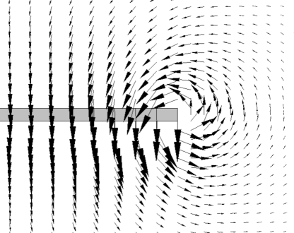
Figure 4: The fluid flow near the tip of the cantilever as illustrated by the velocity vector field calculated from finite element numerical simulations. A cross section of the $x-y$ plane at $z=0$ is shown (see Fig. 1) that is a close-up view of the tip-region. The shaded region indicates the cantilever (because of the small deflections used in the simulations that cantilever does not appear to be deflected). (top) The flow field near the tip of the rectangular cantilever. This flow field is at t=6$\mu$s and the magnitude of the largest velocity vector shown is -0.3 nm/s. (bottom) The flow field near the tip of the V-shaped cantilever. This flow field is at t=7.2$\mu$s and the magnitude of the largest velocity vector shown is -26 nm/s. The shaded region indicates the tip region where the two single arms have merged. The open region to the left is where the two single arms have separated revealing the open region in the interior of the V-shaped cantilever.

As discussed earlier, for long and slender rectangular cantilevers the flow field is often approximated by that of a cylinder of diameter $w$ undergoing transverse oscillations. This approach assumes that the fluid flow is essentially two-dimensional in the $y-z$ plane and neglects any flow over the tip of the cantilever. Figure 4 (top) illustrates this tip flow for the rectangular cantilever using vectors of the fluid velocity in the $x-y$ plane at $z=0$. The figure is a close-up view near the tip of the cantilever. It is evident that the flow over the rectangular cantilever is nearly uniform in the axial direction leading up to the tip. However, near the tip there is a significant tip flow that decays rapidly in the axial direction away from the tip. The increasing significance of the tip flow as the cantilever geometry becomes shorter (for example, by simply decreasing $L$) is not certain and remains an interesting open question. However, for the geometry used here it is clear that this tip-flow is negligible based upon the accuracy of the analytical predictions using the two-dimensional model.

Figure 4 (bottom) illustrates the tip flow for the V-shaped cantilever, again by showing velocity vectors in the $x-y$ plane at $z=0$. The shaded region indicates the part of the cantilever where the two arms have merged. To the right of the shaded region illustrates flow off the tip and to the left indicates flow that circulates back in between the two individual arms.

In order to illustrate the three-dimensional nature of this flow, the flow field in the $y-z$ plane is shown at two axial locations in Fig. 5. Figure 5(top) is at axial location $x=77\mu$m. The two shaded regions indicate the two arms of the cantilever. Each arm is generating a flow with a viscous boundary layer (Stokes layer) as expected from previous work on rectangular cantilevers. However, the Stokes layers interact in a complicated manner near the center. It is expected that as one goes from the base of the cantilever to the tip that these fluid structures would transition from non-interacting to strongly-interacting.

Figure 5(bottom) illustrates the flow field at axial location $x=108.8\mu$m, the axial location at which the two arms of the cantilever merge to form the tip region. The length of the shaded region is therefore $36\mu$m or twice that of a single arm shown in Fig. 5(top). For this tip region the flow field is similar to what would be expected of a single rectangular cantilever of this width.

Overall, it is clear that the fluid flow field is more complex for the V-shaped cantilever than for the long and slender rectangular beam. For the V-shaped cantilever the flow is three-dimensional near the tip region where the two arms join together.

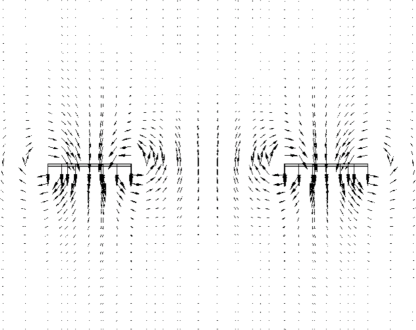
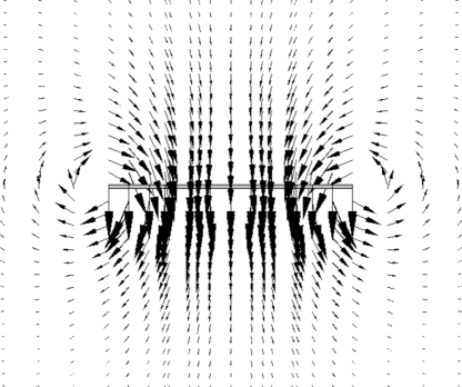
Figure 5: The fluid velocity vector field at two axial positions along the V-shaped cantilever calculated from deterministic finite element numerical simulations. Cross sections of the $y-z$ plane are shown (see Fig. 1), the entire simulation domain is not shown and the shaded region indicates the cantilever. Both images are taken at t=7.2$\mu$s and the maximum velocity vector shown is -26 nm/s. (top) The $y-z$ plane at $x=77\mu$m. The skewed width of a single arm of the cantilever in this cross-section is $18\mu$m. The distance separating the two cantilever arms is $36\mu$m. (bottom) The $y-z$ plane at $x=108.8\mu$m. This is the point at which the two single arms join to make a continuous cross-section of width $2w$.

Central to the flow field dynamics are the interactions of the two Stokes layers caused by the oscillating cantilever arms. The thickness of these Stokes layers are expected to scale with the frequency of oscillation as $\delta_{s}/a\sim{R_{\omega}}^{-1/2}$ where $a$ is the half-width of the cantilever and $R_{\omega}=\omega a^{2}/\nu$ is a frequency based Reynolds number (often called the frequency parameter). For the relevant case of a cylinder of radius $a$ oscillating at frequency $\omega$ the solution to the unsteady Stokes equations yields a distance of approximately $5\delta_{s}$ to capture 99% of the fluid velocity in the viscous boundary layer Carvajal and Paul . For a single arm of the V-shaped cantilever this distance is nearly $10\mu$m. In comparison, the total distance between the two arms at the base is $125\mu$m. This separation is large enough such that the two Stokes layers have negligible interactions near the base. However, as the arms approach one another with axial distance the Stokes layers overlap and eventually merge at the tip.

Despite the complicated interactions of the three-dimensional flow caused by the cantilever tip and the axial merging of the two Stokes layers, the V-shaped cantilever behaves as a damped simple harmonic oscillator. The autocorrelations in tip-angle and tip-displacement that are found using full finite element numerical simulations are shown in Fig. 6. It is again clear that the tip-angle dynamics have significant contributions from the higher modes, see the inset of Fig. 6. The area normalized noise spectra are shown in Fig. 7.

Figure 6: The normalized autocorrelation of equilibrium fluctuations in the tip-deflection $\left<u_{1}(0)u_{1}(t)\right>$ (solid lined) and in tip-angle $\left<\theta_{1}(0)\theta_{1}(t)\right>$ (dashed-line) for the V-shaped cantilever. The inset shows a close-up of the dynamics for short time differences to illustrate the influence of the higher modes in the tip-angle measurements.

Figure 7: The noise spectra for the V-shaped cantilever as determined from the tip-displacement $G_{x}$ (solid line) and from tip-angle $G_{\theta}$ (dashed line). The curves are normalized to have an area of unity, with only the first two modes shown.

Using a simple harmonic oscillator analogy a peak frequency and a quality factor can be determined from the first mode in the noise spectra of Fig. 7. These values are given in the first two rows of Table 6. The quality of the cantilever is $Q\approx 2$ and the peak frequency is reduced significantly, $\omega_{f}/\omega_{0}\approx 0.2$. compared to the resonant frequency in the absence of a surrounding viscous fluid.

It is insightful and of practical use to determine the geometry of the equivalent rectangular beam that would yield the precise values of $k$, $\omega_{f}$, and $Q$ calculated for the V-shaped cantilever from full finite-element numerical simulations. For the rectangular beam the equations are well known (c.f. Ref. Paul et al. (2006)) and yield a unique value of length $L^{\prime}$, width $w^{\prime}$, and height $h^{\prime}$ as shown below,

$$k = \frac{3EI}{L^{\prime 3}}=\frac{Ew^{\prime}h^{\prime 3}}{4L^{\prime 3}},$$ (14)

$$Q = \frac{m_{f}\omega_{f}}{\gamma_{f}}=\frac{\frac{4\rho_{c}h^{\prime}}{\pi\rho_{f}w^{\prime}}+\Gamma^{\prime}(w^{\prime},\omega_{f})}{\Gamma^{\prime\prime}(w^{\prime},\omega_{f})},$$ (15)

where the peak frequency is determined from the maximum of the noise spectrum,

$$G_{u} = \frac{4k_{B}T}{k}\frac{1}{\omega_{0}}$$

$$\times \frac{T_{0}\tilde{\omega}\Gamma^{\prime\prime}(R_{0}\tilde{\omega})}{\left[(1-\tilde{\omega}^{2}(1+T_{0}\Gamma^{\prime}(R_{0}\tilde{\omega})))^{2}+(\tilde{\omega}^{2}T_{0}\Gamma^{\prime\prime}(R_{0}\tilde{\omega}))^{2}\right]}.$$

In the above equations $\tilde{\omega}=\omega/\omega_{0}$ is the normalized frequency, $\alpha=0.234$ is a constant factor to determine an equivalent lumped mass for a rectangular beam, $m_{f}$ is the equivalent mass of the cantilever plus the added fluid mass, $\gamma_{f}$ is the fluid damping, $\Gamma$ is the hydrodynamic function for an infinite cylinder, $\Gamma^{\prime}$ is the real part of $\Gamma$, and $\Gamma^{\prime\prime}$ is the imaginary part of $\Gamma$. Equations (14)-(15) can be solved to yield values for the unknown geometry of the equivalent rectangular beam $L^{\prime}$, $w^{\prime}$, and $h^{\prime}$ which are given in Table 5. The equivalent beam is shorter, thinner, and wider than the V-shaped cantilever. Importantly, the width of the equivalent beam is nearly twice that of a single arm of the V-shaped cantilever.

$L^{\prime}/L$	$w^{\prime}/w$	$h/h^{\prime}$
0.8	1.9	0.8

Table 5: The geometry of the equivalent rectangular beam that yields the exact values of $k$, $\omega_{f}$, and $Q$ for the V-shaped cantilever that have been determined from full finite-element numerical simulations. The length, width, and height of the equivalent beam $(L^{\prime},w^{\prime},h^{\prime})$ are calculated using Eqs. (14)-(15) and are normalized by the values of ($L,w,h$) for the V-shaped cantilever given in Table 1.

These results suggest that the parallel beam approximation (PBA) Albrecht et al. (1990); Sader (1995); Sader and White (1993); Butt et al. (1993) commonly used to determine the spring constant for a V-shaped cantilever may also provide a useful geometry for determining the dynamics of V-shaped cantilevers in fluid. In this approximation the V-shaped cantilever is replaced by an equivalent rectangular beam of length $L$, width $2w$, and height $h$ to yield a simple analytical expression for the spring constant. This has been shown to be quite successful for V-shaped cantilevers that have arms that are not significantly skewed. The results of using the geometry of this approximation to determine $\omega_{f}$ and $Q$ from the two-dimensional cylinder approximation are shown on the third row of Table 6. It is clear that this is quite accurate. It is expected that these results will remain useful for cantilever geometries that do not deviate significantly from that of an equilateral triangle as studied here. An exploration of the breakdown of this approximation is possible using the methods described but is beyond the scope of the current efforts.

	$\omega_{f}/\omega_{0}$	$Q$
(1)	0.21	1.98
(2)	0.22	2.04
(L,2w,h)	0.19	1.98

Table 6: The peak frequency and quality factor of the fundamental mode of the V-shaped cantilever determined by finite element simulations using the thermodynamic approach. (1) is computed using the cantilever tip-displacement due to the removal of a step force. (2) is computed using the cantilever tip-angle due to the removal of a point-torque. The third line represents theoretical predictions using the geometry of an equivalent rectangular beam given by $(L,2w,h)$. The frequency result is normalized by the resonant frequency in vacuum $\omega_{0}$.

VI Quantifying the increased dissipation due to a planar boundary

In practice, the cantilever is never placed in an unbounded fluid and the influence of nearby boundaries must be accounted for to provide a complete description of the dynamics. In many cases the cantilever is purposefully brought near a surface out of experimental interest in order to probe some interaction with the cantilever or to probe the surface itself. To specify our discussion we will consider the situation depicted in Fig. 8 showing a cantilever a distance $s$ from a planar boundary. In the following we study the case where the cantilever exhibits flexural oscillations in the direction perpendicular to the boundary. However, we would like to emphasize that our approach is general and can be used to explore arbitrary cantilever orientations and oscillation directions if desired. The fluid is assumed to be unbounded in all other directions. It is well known that the presence of the boundary will influence the dynamics of the cantilever  Benmouna and Johannsmann (2002); Nnebe and Schneider (2004); Harrison et al. (2007). The result is a reduction in the resonant frequency and quality factor. This has been described theoretically for the case of a long and thin cantilever of simple geometry where the fluid dynamics have been assumed two-dimensional  Clarke et al. (2005, 2006a); Green and Sader (2005a, b).

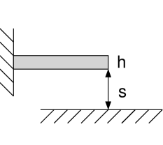
Figure 8: A schematic of a cantilever a distance $s$ away from a solid planar surface (not drawn to scale). The cantilever undergoes flexural oscillations perpendicular to the surface.

In the following we use the thermodynamic approach with finite element numerical simulations to quantify the dynamics of the V-shaped cantilever as a function of its separation from a boundary. We have performed 8 simulations over a range of separations from 10 to 60$\mu$m using both the tip-deflection and tip-angle formulations. The noise spectra for these simulations are shown in Fig. 9. Using the insights from our simulations of the V-shaped cantilever in an unbounded fluid we expect the relevant length scale for the fluid dynamics to be twice the width of a single arm, $2w$. Using the peak frequency of the V-shaped cantilever in unbounded fluid yields a Stokes length $\delta_{s}=4.14\mu$m. Scaling the separation by the Stokes length yields. $2.5\lesssim s/\delta_{s}\lesssim 15$ which covers the range from what is expected to be a strong influence of the wall to a negligible influence. Figure 9 clearly shows a reduction in the peak frequency and a broadening of the peak as the cantilever is brought closer to the boundary. In fact, for the smaller separations the peak is quite broad and the trend suggests that eventually the peak will become annihilated as the cantilever is brought closer to the boundary.

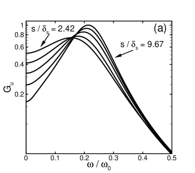
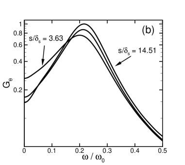
Figure 9: Panel (a) The noise spectra $G_{u}$ of stochastic fluctuations in cantilever tip-deflection for separations $s=10,12,15,20,40\mu$m. Panel (b) the noise spectra $G_{\theta}$ of stochastic fluctuations in cantilever tip-angle for separations $s=15,25,60\mu$m. The spectra have been normalized by the maximum value of $G_{u}$ or $G_{\theta}$. The smallest and largest values of separation are labeled with all other values appearing sequentially.

Using the noise spectra we compute a peak frequency and a quality factor for the fundamental mode as a function of separation from the boundary, which are plotted in Fig. 10. The horizontal dashed line represents the value of the peak frequency and quality factor in the absence of bounding surfaces using the two-dimensional infinite cylinder approximation Paul et al. (2006) where the cylinder width has been chosen to be $2w$. It is clear from the results that for separations greater than $s/\delta_{s}\gtrsim 7$ the V-shaped cantilever is not significantly affected by the presence of the boundary. However, as the separation decreases below this value the peak frequency and quality factor decrease rapidly.

The triangles in Fig. 10 represent the theoretical predictions of Green and Sader Green and Sader (2005a, b) using a two-dimensional approximation for a beam of uniform cross-section that accounts for the presence of the boundary. We have used a width of $2w$ in computing these theoretical predictions for comparison with our numerical results. Despite the complex and three-dimensional nature of the flow field the theory is able to accurately predict the quality factor over the range of separations explored. The frequency of the peak for the V-shaped cantilever shows some deviation from these predictions.

In general, an increase in the period of oscillation for a submerged object can be attributed to the mass of fluid entrained by the object Stokes (1850). The lower peak frequency calculated for the V-shaped cantilever using a two-dimensional solution indicates an over-prediction of the mass loading. This can be attributed to the three-dimensional flow around the tip being neglected for this approach. It is reasonable to expect the cantilever tip to carry a smaller amount of fluid than a section of the beam body moving with the same velocity, see Fig. 4. The quality factor relates to the ratio of the mass loading and the viscous dissipation and is less sensitive to deviations incurred from the two-dimensional approximation. Despite neglecting three-dimensional flow around the cantilever tip, the two-dimensional model for the fluid flow around the V-shaped cantilever gives an accurate prediction of the peak frequency and quality factor.

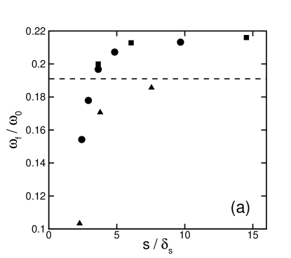
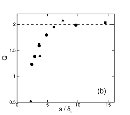
Figure 10: The variation of the peak frequency (panel (a)) and quality (panel (b)) of the fundamental mode of the V-shaped cantilever in fluid as a function of separation from a nearby wall. Results calculated using tip-deflection are circles, results using tip-angle are squares, and theoretical predictions using the results of Ref. Green and Sader (2005b) are triangles. The peak frequency and quality factor of the fundamental mode in an unbounded fluid are $\omega/\omega_{f}\approx 0.19$ and $Q\approx 2$ and are represented by the horizontal dashed line. The distance $s$ is normalized by the Stokes length $\delta_{s}$ where $a=w$ to yield $\delta_{s}=4.14\mu$m.

VII Conclusions

We have shown that the thermodynamic approach is a versatile and powerful method for predicting the stochastic dynamics of cantilevers in fluid for the precise conditions of experiment including complex geometries and the presence of nearby boundaries. Available analytical predictions are for idealized situations including simple geometries where the three-dimensional flow near the cantilever tip has been neglected. Although this has provided significant insight, many situations of experimental interest are more complicated. It is often required to have a quantitative base-line understanding of the cantilever dynamics for the precise conditions of experiment in order to make and interpret measurements in novel situations and in the presence of other phenomena of interest.

We emphasize that by using the fluctuation-dissipation theorem a single deterministic calculation is sufficient to predict the stochastic behavior for all frequencies. Furthermore, the deterministic calculation is computationally inexpensive and does not require special computing resources.

The thermodynamic approach is general in that it can be used to compute the stochastic dynamics of any conjugate pair of variables. We have shown that the stochastic dynamics that are measured depend upon the choice of measurement. This could be exploited in future experiments, for example, to minimize or maximize the significance of the higher mode dynamics by choosing to measure tip-deflection or tip-angle, respectively.

Our results also suggest that despite the complicated three-dimensional nature of the flow field around a V-shaped cantilever, analytical predictions based upon a two-dimensional description are surprisingly accurate if the appropriate length scales are used. We anticipate that these findings will be of immediate use as the atomic force microscope continues to find further use in liquid environments.

Acknowledgments: This research was funded by AFOSR grant no. FA9550-07-1-0222. Early work on this project was funded by a Virginia Tech ASPIRES grant. We would acknowledge many useful interactions with Michael Roukes, Mike Cross, and Sergey Sekatski.

References

- Butt and Jaschke (1995) H.-J. Butt and M. Jaschke, Nanotech. 6, 1 (1995).
- Ekinci and Roukes (2005) K. L. Ekinci and M. L. Roukes, Review of Scientific Instruments 76 (2005).
- Binnig et al. (1986) G. Binnig, C. F. Quate, and C. Gerber, Phys. Rev. Lett. 56, 930 (1986).
- Garcia and Perez (2002) R. Garcia and R. Perez, Surface Science Reports pp. 197–301 (2002).
- Tuck (1969) E. O. Tuck, J. Eng. Math 3, 29 (1969).
- Sader (1998) J. E. Sader, J. Appl. Phys. 84, 64 (1998).
- Clarke et al. (2005) R. J. Clarke, S. M. Cox, P. M. Williams, and O. E. Jensen, J. Fluid Mech. 545, 397 (2005).
- Benmouna and Johannsmann (2002) F. Benmouna and D. Johannsmann, Eur. Phys. J. E 9, 435 (2002).
- Nnebe and Schneider (2004) I. Nnebe and J. W. Schneider, Langmuir 20, 3195 (2004).
- Clarke et al. (2006a) R. J. Clarke, O. Jensen, J. Billingham, A. Pearson, and P. Williams, Phys. Rev. Lett. 96, 050801 (2006a).
- Green and Sader (2005a) C. P. Green and J. E. Sader, Phys. Fluids 17, 073102 (2005a).
- Green and Sader (2005b) C. P. Green and J. E. Sader, J. Appl. Phys. 98, 114913 (2005b).
- Harrison et al. (2007) C. Harrison, E. Tavernier, O. Vancauwenberghe, E. Donzier, K. Hsu, A. Goodwin, F. Marty, and B. Mercier, Sensor and Actuators A 134, 414 (2007).
- Clarke et al. (2006b) R. J. Clarke, O. Jensen, J. Billingham, and P. Williams, Proc. R. Soc. A 462, 913 (2006b).
- Paul and Cross (2004) M. R. Paul and M. C. Cross, Physical Review Letters 92(23), 235501 (2004).
- Paul et al. (2006) M. R. Paul, M. Clark, and M. C. Cross, Nanotechnology 17, 4502 (2006).
- Arlett et al. (2006) J. L. Arlett, J. R. Maloney, B. Gudlewski, M. Muluneh, and M. L. Roukes, Nano Lett. 6, 1000 (2006).
- (18) Veeco Probes, www.veecoprobes.com.
- Landau and Lifshitz (1959) L. D. Landau and E. M. Lifshitz, Theory of elasticity (Butterworth-Heinemann, 1959).
- Stark et al. (2001) R. Stark, T. Drobek, and W. Heckl, Ultramicroscopy 86, 207 (2001).
- Yang and Makhijani (1994) H. Q. Yang and V. B. Makhijani, AIAA-94-0179 pp. 1–10 (1994).
- (22) ESI CFD Headquarters, Huntsville AL 25806. We use the CFD-ACE+ solver.
- Chon et al. (2000) J. W. M. Chon, M. P., and J. E. Sader, Journal of Applied Physics 87(8), 3978 (2000).
- Clark and Paul (2006) M. T. Clark and M. R. Paul, Int. J. Nonlin. Mech. (2006).
- (25) C. Carvajal and M. R. Paul, unpublished.
- Albrecht et al. (1990) T. R. Albrecht, S. Akamine, and C. F. Carver, T. S. amd Quate, J. Vac. Sci. Technol. A 8, 3386 (1990).
- Sader (1995) J. E. Sader, Rev. Sci. Instrum. 66, 4583 (1995).
- Sader and White (1993) J. E. Sader and L. White, J. Appl. Phys 74, 1 (1993).
- Butt et al. (1993) H. Butt, P. Siedle, K. Seifert, K. Fendler, T. Seeger, E. Bamberg, A. Weisenhorn, K. Goldie, and A. Engel, J. Microsc. 169, 75 (1993).
- Stokes (1850) S. G. Stokes, Trans. Camb. Phil. Soc. 9, 8 (1850).