Plane geometry and convexity
of polynomial stability regions¹

Abstract

The set of controllers stabilizing a linear system is generally non-convex in the parameter space. In the case of two-parameter controller design (e.g. PI control or static output feedback with one input and two outputs), we observe however that quite often for benchmark problem instances, the set of stabilizing controllers seems to be convex. In this note we use elementary techniques from real algebraic geometry (resultants and Bézoutian matrices) to explain this phenomenon. As a byproduct, we derive a convex linear matrix inequality (LMI) formulation of two-parameter fixed-order controller design problem, when possible.

Keywords
control theory; convexity; resultants

1 Introduction

Despite its elementary formulation, the problem of fixed-order controller design for linear time-invariant systems remains mostly open. Especially scarce are numerically efficient computer-aided control system design algorithms in the fixed-order case, sharply contrasting with the large number of tools available to solve static state feedback design or dynamical output feedback design with controllers of the same order as the plant. Mathematically, fixed-order controller design can be formulated as a non-convex non-smooth optimization problem in the parameter space. To the best of our knowledge, randomized algorithms are amongst the most efficient numerical methods to cope with this class of difficult problems. See [4, 13] for computer experiments supporting this claim, thanks to public-domain Matlab packages (HIFOO and the Randomized Control System Toolbox).

This note was motivated by the observation, made by the first author during a workshop at AIM in August 2005 [8], that 6 out of the 7 two-dimensional instances of static output feedback (SOF) design problems found in the database COMPleib [10] seem to be convex. Further motivation was provided by the excellent historical survey [7] on D-decomposition techniques, previously studied in deep detail in [12] and [1]. In [7] the authors describe the intricate geometry of two-dimensional stability regions with the help of illustrative examples. Quite often, the stability regions represented in these references seem to be convex.

In this note, we use basic results from real algebraic geometry to detect convexity of the stability region in the two-parameter case (including PI controllers, PID with constant gain, SOF design with one input two outputs or two inputs one output). We also derive, when possible, a linear matrix inequality (LMI) formulation of the stability region.

2 Problem statement

We consider a parametrized polynomial

$$p(s,k)=p_{0}(s)+k_{1}p_{1}(s)+k_{2}p_{2}(s)$$ (1)

where the $p_{i}(s)\in{\mathbb{R}}[s]$ are given polynomials of $s\in{\mathbb{C}}$ and the $k_{i}\in{\mathbb{R}}$ are parameters. We assume, without loss of generality, that the ratio $p_{1}(s)/p_{2}(s)$ is not a constant.

Define the stability region

$${\mathcal{S}}=\{k\in{\mathbb{R}}^{2}\>:\>p(s,k)\>\>\mathrm{stable}\}$$

where stability is meant in the continuous-time sense, i.e. all the roots of $p(s,k)$ must lie in the open left half-plane.

We are interested in the following problems:

• Is stability region $\mathcal{S}$ convex ?

• If it is convex, give an LMI representation

  $${\mathcal{S}}=\{k\in{\mathbb{R}}^{2}\>:\>F_{0}+F_{1}k_{1}+F_{2}k_{2}\succ 0\}$$

  when possible, where the $F_{i}$ are real symmetric matrices to be found, and $\succ 0$ means positive definite.

2.1 Example: PI controller design

Let $b(s)/a(s)$ with $a(s),b(s)\in{\mathbb{R}}[s]$ denote the transfer function of an open loop plant, and consider a proportional integral (PI) controller $k_{1}/s+k_{2}$ in a standard negative feedback configuration. The closed-loop characteristic polynomial (1) is then $p(s,k)=sa(s)+(k_{1}+k_{2}s)b(s)$ hence $p_{0}(s)=sa(s)$, $p_{1}(s)=b(s)$ and $p_{2}(s)=sb(s)$.

2.2 Example: static output feedback

Given matrices $A\in{\mathbb{R}}^{n\times n}$, $B\in{\mathbb{R}}^{n\times m}$, $C\in{\mathbb{R}}^{p\times n}$, we want to find a matrix $K\in{\mathbb{R}}^{m\times p}$ such that the closed-loop matrix $A+BKC$ is stable. When $mp=2$, the characteristic polynomial (1) writes $p(s,k)=\det(sI_{n}-A-BKC)$ hence $p_{0}(s)=\det(sI_{n}-A)$, $p_{1}(s)=\det(sI_{n}-B[k_{1},0]C)$ and $p_{2}(s)=\det(sI_{n}-B[0,k_{2}]C)$.

3 Hermite matrix

The Routh-Hurwitz criterion for stability of polynomials has a symmetric version called the Hermite criterion. A polynomial is stable if and only if its Hermite matrix, quadratic in the polynomial coefficients, is positive definite. In control systems terminology, the Hermite matrix is a particular choice of a Lyapunov matrix certifying stability [11]. Algebraically, the Hermite matrix can be defined via the Bézoutian, a symmetric form of the resultant [6, Section 5.1.2].

Let $a(u)$, $b(u)$ be two polynomials of degree $n$ of the indeterminate $u$. Define the Bézoutian matrix $B_{u}(a,b)$ as the symmetric matrix of size $n$ with entries $b_{ij}$ satisfying the linear equations

$$\frac{a(u)b(v)-a(v)b(u)}{v-u}=\sum_{i=1}^{n}\sum_{j=1}^{n}b_{ij}u^{i-1}v^{j-1}.$$

The polynomial $r_{u}(a,b)=\det B_{u}(a,b)$ is the resultant of $a(u)$ and $b(u)$ with respect to $u$. It is obtained by eliminating $u$ from the system of equations $a(u)=b(u)=0$.

The Hermite matrix of $p(s)$ is defined as the Bézoutian matrix of the real part and the imaginary part of $p(j\omega)$:

$$\begin{array}[]{rcl}p_{R}(\omega^{2})&=&\mathrm{Re}\>p(j\omega)\\ \omega p_{I}(\omega^{2})&=&\mathrm{Im}\>p(j\omega)\end{array}$$

that is, $H(p)=B_{\omega}(p_{R}(\omega^{2}),\omega p_{I}(\omega^{2}))$. Let us assume that $p(s)$ is monic, with unit leading coefficient. The Hermite stability criterion can be formulated as follows.

Lemma 1

Polynomial $p(s)$ is stable if and only if $H(p)\succ 0$.

Proof: The proof of this result can be found in [11] for example. It can also be proved via Cauchy indices and Hermite quadratic forms for counting real roots of polynomials, see [3, Section 9.3] $\Box$.

By construction, the Hermite matrix of parametrized polynomial (1)

$$H(p(s,k))=H(k)=\sum_{i_{1},i_{2}=0}^{2}H_{i_{1}i_{2}}k_{1}^{i_{1}}k_{2}^{i_{2}}$$

is quadratic in $k$. Therefore, the Hermite criterion yields a quadratic matrix inequality formulation of the stability region:

$${\mathcal{S}}=\{k\in{\mathbb{R}}^{2}\>:\>H(k)\succ 0\}.$$

Quadratic matrix inequalities, a generalization of bilinear matrix inequalities, typically generate non-convex regions. For example, the scalar quadratic inequality $k_{1}^{2}-1>0$ models a disconnected, hence non-convex set.

Surprisingly, it turns out that $\mathcal{S}$, even though modeled by a quadratic matrix inequality, is often a convex set for practical problem instances. Here are some examples.

3.1 Examples: static output feedback

Consider the 7 two-parameter SOF problems found in the database COMPleib [10], labelled AC4, AC7, AC17, NN1, NN5, NN17 and HE1. Stability regions are represented as shaded gray areas on Figures 3 to 7. Visual inspection reveals that 6 out of 7 stability regions seem to be convex. The only apparently nonconvex example is HE1.

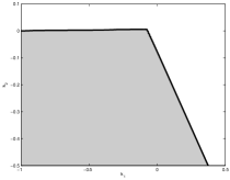
Figure 1: AC4.

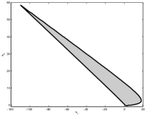
Figure 2: AC7.

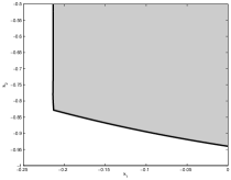
Figure 3: AC17.

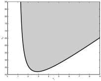
Figure 4: NN1.

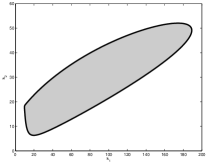
Figure 5: NN5.

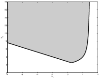
Figure 6: NN17.

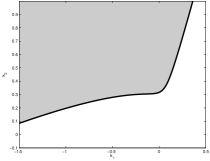
Figure 7: HE1.

In the remainder of the paper we will explain why such planar stability regions are likely to be convex, and how we can constructively derive their LMI formulations when possible.

4 Rational boundary of the stability region

Define the curve

$${\mathcal{C}}=\{k\in{\mathbb{R}}^{2}:p(j\omega,k)=0,w\in{\mathbb{R}}\}$$

which is the set of parameters $k$ for which polynomial $p(s,k)$ has a root along the boundary of the stability region, namely the imaginary axis. Studying this curve is the key idea behind the D-decomposition approach [7]. The curve partitions the plane $(k_{1},k_{2})$ into regions in which the number of stable roots of $p(s,k)$ remains constant. The union of regions for which this number is equal to the degree of $p(s,k)$ is the stability region $\mathcal{S}$. Hence the boundary of $\mathcal{S}$ is included in curve $\mathcal{C}$.

Note that $p(j\omega,k)=0$ for some $w\in{\mathbb{R}}$ if and only if

$$\begin{array}[]{rclcl}p_{R}(\omega^{2},k)&=&p_{0R}(\omega^{2})+k_{1}p_{1R}(\omega^{2})+k_{2}p_{2R}(\omega^{2})&=&0\\ \omega p_{I}(\omega^{2},k)&=&\omega p_{0I}(\omega)+k_{1}\omega p_{1I}(\omega)+k_{2}\omega p_{2I}(\omega)&=&0\\ \end{array}$$

Recall that we denote by $r_{\omega}(q_{1},q_{2})$ the resultant of polynomials $q_{1}(\omega)$,$q_{2}(\omega)$ obtained by eliminating the scalar indeterminate $\omega$. From the definition of the Hermite matrix, it holds

$$h(k)=r_{\omega}(p_{R}(\omega^{2},k),\omega p_{I}(\omega^{2},k))=\det H(k)$$ (2)

from which the implicit algebraic description

$${\mathcal{C}}=\{k:h(k)=0\}$$

follows.

Lemma 2

The determinant of the Hermite matrix can be factored as

$$h(k)=l(k)g(k)^{2}$$

where $l(k)$ is affine, and $g(k)$ is a generically irreducible polynomial.

Proof: The result follows from basic properties of resultants: $h(k)=r_{\omega}(p_{R}(\omega^{2},k),\omega p_{I}(\omega^{2},k))=r_{\omega}(p_{R}(\omega^{2},k),\omega^{2})r_{\omega}(p_{R}(\omega^{2},k),p_{I}(\omega^{2},k))=r_{\omega}(p_{R}(\omega,k),\omega)r_{\omega}(p_{R}(\omega,k),p_{I}(\omega,k))^{2}$. Take $g(k)=r_{\omega}(p_{R}(\omega,k),p_{I}(\omega,k))$. Since $p_{R}(\omega,k)$ is affine in $k$ it follows that $l(k)=r_{\omega}(p_{R}(\omega,k),\omega)$ is affine in $k$.$\Box$

The curve can therefore be decomposed as the union of a line and a simpler algebraic curve

$${\mathcal{C}}={\mathcal{L}}\cup{\mathcal{G}}=\{k:l(k)=0\}\cup\{k:g(k)=0\}.$$

The equation of line $\mathcal{L}$ was already given in the proof of Lemma 2, namely

$$l(k)=r_{\omega}(p_{R}(\omega),\omega)=p_{R}(0,k)=p_{0R}(0)+k_{1}p_{1R}(0)+k_{2}p_{2R}(0).$$

The defining polynomial of the other curve component $\mathcal{G}$ can be obtained via the formula

$$g(k)=r_{\omega}(p_{R}(\omega,k),p_{I}(\omega,k)).$$

From the relations

$$\left[\begin{array}[]{cc}p_{1R}(\omega^{2})&p_{2R}(\omega^{2})\\ \omega p_{1I}(\omega^{2})&\omega p_{2I}(\omega^{2})\end{array}\right]\left[\begin{array}[]{c}k_{1}\\ k_{2}\end{array}\right]=-\left[\begin{array}[]{c}p_{0R}(\omega^{2})\\ \omega p_{0I}(\omega^{2})\end{array}\right]$$

we derive a rational parametrization of $\mathcal{G}$:

$$\left[\begin{array}[]{c}k_{1}(\omega^{2})\\ k_{2}(\omega^{2})\end{array}\right]=\frac{\left[\begin{array}[]{cc}p_{2I}(\omega^{2})&-p_{2R}(\omega^{2})\\ -p_{1I}(\omega^{2})&p_{1R}(\omega^{2})\end{array}\right]}{p_{1I}(\omega^{2})p_{2R}(\omega^{2})-p_{1R}(\omega^{2})p_{2I}(\omega^{2})}\left[\begin{array}[]{c}p_{0R}(\omega^{2})\\ p_{0I}(\omega^{2})\end{array}\right]=\left[\begin{array}[]{c}\frac{q_{1}(\omega^{2})}{q_{0}(\omega^{2})}\\ \frac{q_{2}(\omega^{2})}{q_{0}(\omega^{2})}\\ \end{array}\right]$$ (3)

which is well-defined since by assumption $p_{1}(s)/p_{2}(s)$ is not a constant. From this parametrization we can derive a symmetric linear determinantal form of the implicit equation of this curve.

Lemma 3

The symmetric affine pencil

$$G(k)=B_{\omega}(q_{1},q_{2})+k_{1}B_{\omega}(q_{2},q_{0})+k_{2}B_{\omega}(q_{1},q_{0}).$$

is such that ${\mathcal{G}}=\{k:\det G(k)=0\}$.

Proof: Rewrite the system of equations (3) as

$$\begin{array}[]{rcccl}a(\omega^{2},k)&=&q_{1}(\omega^{2})-k_{1}q_{0}(\omega^{2})&=&0\\ b(\omega^{2},k)&=&q_{2}(\omega^{2})-k_{2}q_{0}(\omega^{2})&=&0\\ \end{array}$$

and use the Bézoutian resultant to eliminate indeterminate $\omega$ and obtain conditions for a point $(k_{1},k_{2})$ to belong to the curve. The Bézoutian matrix is $B_{\omega}(a,b)=B_{\omega}(q_{1}-k_{1}q_{0},q_{2}-k_{2}q_{0})=B_{\omega}(q_{1},q_{2})+k_{1}B_{\omega}(q_{2},q_{0})+k_{2}B(q_{1},q_{0})$. Linearity in $k$ follows from bilinearity of the Bézoutian and the common factor $q_{0}$.$\Box$

Finally, let $C(k)=\mathrm{diag}\>\{l(k),G(k)\}$ so that curve $\mathcal{C}$ can be described as a determinantal locus

$${\mathcal{C}}=\{k\>:\>\det C(k)=0\}.$$

5 LMI formulation

Curve $\mathcal{C}$ partitions the plane into several connected components, that we denote by ${\mathcal{S}}_{i}$ for $i=1,\ldots,N$.

Lemma 4

If $C(k)\succ 0$ for some point $k$ in the interior of ${\mathcal{S}}_{i}$ for some $i$ then ${\mathcal{S}}_{i}=\{k:C(k)\succeq 0\}$ is a convex LMI region.

Proof: Follows readily from the affine dependence of $C(k)$ on $k$ and from the fact that the boundary of ${\mathcal{S}}_{i}$ is included in $\mathcal{C}$. $\Box$

Convex sets which admit an LMI representation are called rigidly convex in [9]. Rigid convexity is stronger than convexity. It may happen that ${\mathcal{S}}_{i}$ is convex for some $i$, yet $C(k)$ is not positive definite for points $k$ within ${\mathcal{S}}_{i}$.

Lemma 5

Stability region $\mathcal{S}$ is the union of sets ${\mathcal{S}}_{i}$ containing points $k$ such that $H(k)\succ 0$.

Proof: Follows readily from Lemma 1.$\Box$

Note that it may happen that ${\mathcal{S}}_{i}$ is convex LMI for some $i$, yet $H(k)$ is not positive definite for points $k$ within ${\mathcal{S}}_{i}$.

Corollary 1

If $H(k)\succ 0$ and $C(k)\succ 0$ for some point $k$ in the interior of ${\mathcal{S}}_{i}$, then ${\mathcal{S}}_{i}$ is an LMI region included in the stability region.

Proof: Combine Lemmas 4 and 5.$\Box$

Quite often, on practical instances, we observe that ${\mathcal{S}}={\mathcal{S}}_{i}$ for some $i$ is a convex LMI region.

Practically speaking, once curve $\mathcal{C}$ is expressed as a determinantal locus, the search of points $k$ such that $C(k)\succ 0$ can be formulated as an eigenvalue problem, but this is out of the scope of this paper.

6 Examples

6.1 Example 1

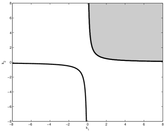
Figure 8: Vishnegradsky’s degree 3 polynomial. Rational curve $\mathcal{C}$ with convex LMI stability region $\mathcal{S}$ (in gray)

As mentioned in [7], Vishnegradsky in 1876 considered the polynomial $p(s,k)=s^{3}+k_{1}s^{2}+k_{2}s+1$ and concluded that its stability region ${\mathcal{S}}=\{k:k_{1}>0,k_{1}k_{2}>1\}$ is convex hyperbolic.

The Hermite matrix of $p(s,k)$ is given by

$$H(k)=\left[\begin{array}[]{ccc}k_{2}&0&1\\ 0&k_{1}k_{2}-1&0\\ 1&0&k_{1}\end{array}\right]$$

and hence after a row and column permutation the quadratic matrix inequality formulation

$${\mathcal{S}}=\{k:\left[\begin{array}[]{ccc}k_{2}&1&0\\ 1&k_{1}&0\\ 0&0&k_{1}k_{2}-1\end{array}\right]\succ 0\}$$

explains why the region is convex. Indeed, the determinant of the 2-by-2 upper matrix, affine in $k$, is equal to the remaining diagonal entry, which is here redundant. The stability region can therefore be modeled as the LMI

$${\mathcal{S}}=\{k:\left[\begin{array}[]{cc}k_{1}&1\\ 1&k_{2}\end{array}\right]\succ 0\}$$

see Figure 8.

6.2 Example 2

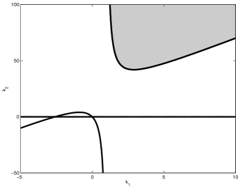
Figure 9: NN1 SOF example. Rational curve $\mathcal{C}$ with convex LMI stability region $\mathcal{S}$ (in gray)

Consider problem NN1 from [10], for which $p_{0}(s)=s(s^{2}-13)$, $p_{1}(s)=s(s-5)$, $p_{2}(s)=s+1$ in (1). We have $p_{R}(\omega^{2})=-k_{1}\omega^{2}+k_{2}$ and $p_{I}(\omega^{2})=-\omega^{2}-13-5k_{1}+k_{2}$ and

$$H(k)=\left[\begin{array}[]{ccc}k_{2}(-13-5k_{1}+k_{2})&0&-k_{2}\\ 0&k_{1}(-13-5k_{1}+k_{2})-k_{2}&0\\ -k_{2}&0&k_{1}\end{array}\right].$$

Hence $h(k)=\det H(k)=k_{2}(-13k_{1}-k_{2}-5k_{1}^{2}+k_{1}k_{2})^{2}$ and then $l(k)=k_{2}$, $g(k)=-13k_{1}-k_{2}-5k_{1}^{2}+k_{1}k_{2}$. A rational parametrization of the curve ${\mathcal{G}}=\{k:g(k)=0\}$ is given by

$$\begin{array}[]{rcl}k_{1}(\omega^{2})&=&(\omega^{2}+13)/(\omega^{2}-5)\\ k_{2}(\omega^{2})&=&\omega^{2}(\omega^{2}+13)/(\omega^{2}-5)\end{array}$$

from which we derive the symmetric affine determinantal representation ${\mathcal{G}}=\{k:\det G(k)=0\}$ with

$$G(k)=\left[\begin{array}[]{cc}169+65k_{1}-18k_{2}&13+5k_{1}\\ 13+5k_{1}&1-k_{1}\end{array}\right].$$

The pencil representing $\mathcal{C}$ is therefore

$$C(k)=\left[\begin{array}[]{ccc}k_{2}&0&0\\ 0&169+65k_{1}-18k_{2}&13+5k_{1}\\ 0&13+5k_{1}&1-k_{1}\end{array}\right].$$

We can check that ${\mathcal{S}}=\{k:C(k)\succ 0\}$ is a convex LMI formulation of the stability region represented on Figure 6. Compare with Figure 9 where we represent also the curve ${\mathcal{C}}=\{k:\det C(k)=0\}$.

6.3 Example 3

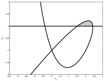
Figure 10: Francis’ example. Rational curve $\mathcal{C}$ with convex LMI stability region $\mathcal{S}$ (in gray)

This example, originally from Francis (1987), is also described in [7]. A SISO plant $(s-1)(s-2)/(s+1)(s^{2}+s+1)$ must be stabilized with a PI controller $k_{1}+k_{2}/s$. Equivalently, $p_{0}(s)=s(s+1)(s^{2}+s+1)$, $p_{1}(s)=s(s-1)(s-2)$ and $p_{2}(s)=(s-1)(s-2)$ in (1).

For these values we obtain

$$C(k)=\left[\begin{array}[]{cccc}2k_{2}&0&0&0\\ 0&14+28k_{1}-54k_{2}&-20-40k_{1}+18k_{2}&2+4k_{1}\\ 0&-20-40k_{1}+18k_{2}&77-53k_{1}+36k_{2}&-11+5k_{1}\\ 0&2+4k_{1}&-11+5k_{1}&5+k_{1}\end{array}\right]$$

and the LMI stability region ${\mathcal{S}}=\{k:C(k)\succ 0\}$ represented on Figure 10 together with the quartic curve ${\mathcal{C}}=\{k:\det C(k)=0\}$.

6.4 Example 4

Consider [1, Example 14.4] for which $p_{0}(s)=s^{4}+2s^{3}+10s^{2}+10s+14+2a$, $p_{1}(s)=2s^{3}+2s-3/10$, $p_{2}(s)=2s+1$, with $a\in{\mathbb{R}}$ a parameter.

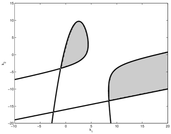
Figure 11: Ackermann’s example with $a=1$. Rational curve $\mathcal{C}$ and stability region $\mathcal{S}$ consisting of two disconnected regions (in gray), the one including the origin being LMI.

We obtain $C(k)=\mathrm{diag}\>\{l(k),G(k)\}$ with

$$\begin{array}[]{rcl}l(k)&=&140+20a-3k_{1}+10k_{2}\\[10.00002pt] G(k)&=&\left[\begin{array}[]{ccc}\begin{array}[]{c}7920+4860a+400a^{2}\\ +(-1609-60a)k_{1}+(-270+200a)k_{2}\end{array}&\star&\star\\ -8350-2000a+1430k_{1}+130k_{2}&8370-1230k_{1}-100k_{2}&\star\\ 900+200a-130k_{1}&-900+100k_{1}&100\end{array}\right]\end{array}$$

where symmetric entries are denoted by stars.

When $a=1$, the stability region consists of two disconnected components. The one containing the origin $k_{1}=k_{2}=0$ is the LMI region $\{k:C(k)\succ 0\}$, see Figure 11.

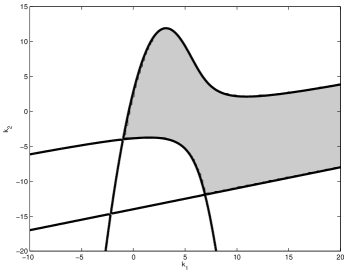
Figure 12: Ackermann’s example with $a=0$. Rational curve $\mathcal{C}$ and non-convex stability region $\mathcal{S}$ (in gray).

When $a=0$, the stability region $\mathcal{S}$ is the non-convex region represented on Figure 12. The LMI region $\{k:C(k)\succ 0\}$ is not included in $\mathcal{S}$ in this case.

7 Conclusion

In this paper we have explained why the planar stability region of a polynomial may be convex with an explicit LMI representation. This is an instance of hidden convexity of a set which is otherwise described by intersecting (generally non-convex) Routh-Hurwitz minors sublevel sets or by enforcing positive definiteness of a (generally non-convex) quadratic Hermite matrix.

Practically speaking, optimizing a closed-loop performance criterion over an LMI formulation of the stability region is much simpler than optimizing over the non-linear formulation stemming from the Routh-Hurwitz minors or the Hermite quadratic matrix inequality.

Convexity in the parameter space was already exploited in [5, 2] in the context of PID controller design. It was shown that when the proportional gain is fixed, the set of integral and derivative gains is a union of a finite number of polytopes.

Extension of these ideas to the case of more than 2 parameters seems to be difficult. The problem of finding a symmetric affine determinantal representation of rationally parametrized surfaces or hypersurfaces is not yet well understood, to the best of our knowledge. For example, in the simplest third degree case $p(s,k)=s^{3}+k_{1}s^{2}+k_{2}s+k_{3}$, how could we find four symmetric real matrices $A_{0}$, $A_{1}$, $A_{2}$, $A_{3}$ satisfying $\det(A_{0}+A_{1}k_{1}+A_{2}k_{2}+A_{3}k_{3})=k_{1}k_{3}-k_{2}$ ?

References

- [1] J. Ackermann et al. Robust control: the parameter space approach. Springer, 1993.
- [2] J. Ackermann, D. Kaesbauer. Stable polyhedra in parameter space. Automatica, 39:937–943, 2003.
- [3] S. Basu, R. Pollack, M.-F. Roy. Algorithms in real algebraic geometry. Springer, 2003.
- [4] J. V. Burke, D. Henrion, A. S. Lewis, M. L. Overton. Stabilization via nonsmooth, nonconvex optimization. IEEE Trans. Autom. Control, 51(11):1760–1769, 2006.
- [5] A. Datta, A. Ho, S. P. Bhatthacharyya. Structure and synthesis of PID controllers. Springer, 2000.
- [6] M. Elkadi, B. Mourrain. Introduction à la résolution des systèmes polynomiaux. Springer, 2007.
- [7] E. N. Gryazina, B. T. Polyak. Stability regions in the parameter space: D-decomposition revisited. Automatica, 42(1):13–26, 2006.
- [8] J. W. Helton, P. A. Parrilo, M. Putinar. Theory and algorithms of linear matrix inequalities - questions and discussions of the literature. Compiled by S. Prajna. The American Institute of Mathematics, Palo Alto, USA, March 2006.
- [9] J. W. Helton, V. Vinnikov. Linear matrix inequality representation of sets. Comm. Pure Applied Math. 60(5):654-674, 2007.
- [10] F. Leibfritz. COMPleib: constraint matrix optimization problem library - a collection of test examples for nonlinear semidefinite programs, control system design and related problems. Technical Report, Univ. Trier, Germany, 2004.
- [11] P. C. Parks, V. Hahn. Stability theory. Prentice Hall, 1993. Original version published in German in 1981.
- [12] D. D. Šiljak. Parameter space methods for robust control design: a guided tour. IEEE Trans. Autom. Control, 34(7):674–688, 1989.
- [13] R. Tempo, G. Calafiore. F. Dabbene. Randomized algorithms for analysis and control of uncertain systems. Springer, 2005.