Mona Lisa
the stochastic view and fractality in color space

Abstract

A painting consists of objects which are arranged in specific ways. The art of painting is drawing the objects, which can be considered as known trends, in an expressive manner. Detrended methods are suitable for characterizing the artistic works of the painter by eliminating trends. It means that we study the paintings, regardless of its apparent purpose, as a stochastic process. We apply multifractal detrended fluctuation analysis to characterize the statistical properties of Mona Lisa, as an instance, to exhibit the fractality of the painting. Our results show that Mona Lisa is long range correlated and almost behaves similar in various scales.

Pacs:02.50.Fz, 05.45.Tp

Keywords: Painting, Stochastic analysis, Time series analysis

1 Introduction

Art is a collection of objects created with the intention of transmitting emotions and/or ideas. An object can be characterized by intentions of its creator, regardless of its apparent purpose. In this sense, art is described as a deliberate process of arrangement by an agent. Art stimulates an individual’s thoughts, emotions, beliefs, or ideas through the senses. It is also an expression of an idea and it can take many different forms and serve many different purposes. Mathematics and art are examples of human motivations to understand reality [1, 2, 3, 4, 5, 6]. The connection between mathematics and art goes back to thousands of years. Patterns, symmetries, proportions and transformations are fundamental concepts common to both disciplines. One of the connections between mathematics and art is that some known as artists have needed to develop or use mathematical thinking to carry out their artistic insight. Thus we are forced to use interpretative techniques in order to search for them. In particular, there are several obvious relations between art and mathematics such as music [3, 5, 6, 7, 8, 9] and painting [1, 4, 10, 11, 2, 12, 13, 14].

Painting has three principal parts: drawing, proportion and coloring. Drawing is outlines and contours contained in a painting. Proportion is these outlines and contours positioned in proportion in their places. Coloring is giving colors to things. One can obviously use mathematical geometry to analyze paintings, figurative or abstract, in terms of shapes such as points and lines, circles and triangles. One may think of the application of the perspective theory to figurative painting, or the use of some concepts like fractals for comprehension of abstract paintings. An important example is the analysis of Jackson Pollock’s drip paintings in terms of fractal geometry [1].

Here, we are interested to study the fractal nature of painting from another point of view which in general, could be applicable to non-stationary series [3]. Among various paintings we focus on characterizing the complexity of color signal of “Mona Lisa” through computation of signal parameters and scaling exponents, which quantifies correlation exponents and multifractality of the signal.

Mona Lisa, or La Gioconda (La Joconde), is a 16th century oil painting on poplar wood by Leonardo da Vinci, and is the most famous painting in the world. This painting is a half-length portrait which depicts a woman whose gaze meets the viewer’s with an enigmatic expression (Fig. 1). Because of non-stationary nature of color signal series, and due to finiteness of available data sample, we should apply methods which are insensitive to non-stationarities, like trends. In order to separate trends from correlations we need to eliminate trends in our color data. Several methods are used effectively for this purpose: detrended fluctuation analysis (DFA) [15], rescaled range analysis (R/S) [16] and wavelet techniques (WT) [17]. However, using increment series is customary to make a stationary series from a non-stationary ones [18].

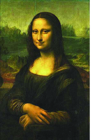
Figure 1: Mona Lisa: oil painting on poplar wood by Leonardo da Vinci.

We use MF-DFA method for analysis and eliminating trends from data set. This method is the modified version of DFA method to detect multifractal properties of time series. DFA method introduced by Peng et al. [15] has become a widely used technique for the determination of monofractal scaling properties and the detection of long-range correlations in noisy, non-stationary time series [19, 20, 21, 22]. It has successfully been applied to diverse fields [15, 23, 24, 25, 26, 27, 3, 28, 29, 30, 31]. One reason to employ DFA method is to avoid spurious detection of correlations that are artefacts of non-stationarity series. The focus of the present paper is on the fractality nature of color series obtained from Mona Lisa. To construct the series, we calculate the standard color values of each pixel of the picture successively for each row from up to down, continuously. In particular, Fig. 1 shows Mona Lisa and Fig. 2 shows its gray, red, green and blue color styles for a $202\times 300$ pixels sample. The color fluctuation graphs of gray and red styles, are also depicted in Fig. 3.

The paper is organized as follows: In Sec. 2, we describe MF-DFA methods in detail and show that scaling exponents determined by MF-DFA method are identical to those obtained by standard multifractal formalism based on partition functions. In Sec. 3, in analysis of color series of Mona Lisa we also examine the multifractality in color data. Section 4 closes with a conclusion.

2 Multifractal Detrended Fluctuation Analysis

The simplest type of multifractal analysis is based upon standard partition function multifractal formalism, which has been developed for multifractal characterization of normalized, stationary measurements [32, 33, 34, 35]. Unfortunately, this standard formalism does not give us correct results for non-stationary time series that are affected by trends or those which cannot be normalized. MF-DFA is based on identification of scaling of $q$th-order moment depending on signal length, and this is a generalization of standard DFA method in which $q=2$. Moreover one should find correct scaling behavior of fluctuations, from experimental data which are often affected by non-stationary sources, like trends. These have to be well distinguished from intrinsic fluctuations of the system. In addition, often in collected data we do not know the reasons, or even worse the scales, for underlying trends, and also available record data is usually small. So, for a reliable detection of correlations, it is essential to distinguish trends for intrinsic fluctuations from collected data. Hurst rescaled-range analysis [16] and other non-detrending methods work well when records are long and do not involve trends, otherwise they might give wrong results. DFA is a well established method for determining scaling behavior of noisy data where the data include trends and their origin and shape are unknown [15, 25, 36, 37, 23].

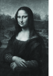
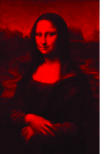
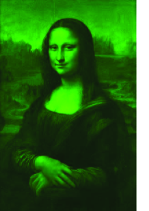
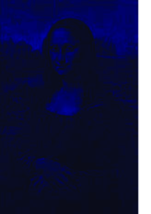
Figure 2: Gray, red, green and blue style pictures (up to down respectively) of Mona Lisa

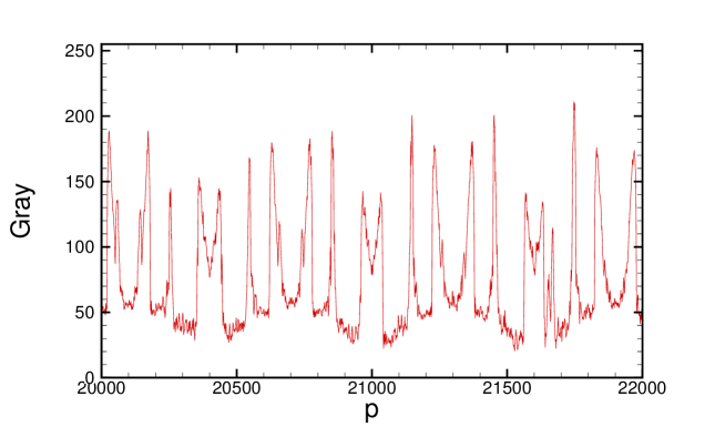
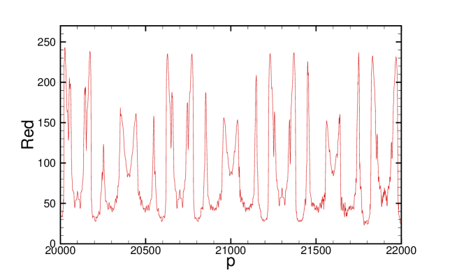
Figure 3: Typical color value of color series for gray (Up) and red (Down) style.

Modified multifractal DFA procedure consists of five steps. The first three steps are essentially identical to conventional DFA procedure (see e.g. [15, 19, 20, 21, 22]). Suppose that $x_{k}$ is a series of length $N$, and it is of compact support, i.e. $x_{k}=0$ for an insignificant fraction of the values only.

$\bullet$ Step 1: Determine the profile

$$Y(i)\equiv\sum_{k=1}^{i}\left[x_{k}-\langle x\rangle\right],\qquad i=1,\ldots,N.$$ (1)

Subtraction of the mean $\langle x\rangle$ from $x_{k}$ is not compulsory, since it would be eliminated by later detrending in third step.

$\bullet$ Step 2: Divide profile $Y(i)$ into $N_{s}\equiv{\rm int}(N/s)$ non-overlapping segments of equal lengths $s$. Since length $N$ of series is often not a multiple of considered time scale $s$, a short part at the end of profile may remain. In order not to disregard this part of the series, same procedure should be repeated starting from the opposite end.

$\bullet$ Step 3: Calculate local trend for each of $N_{s}$ segments by a least-square fit of the series. Then determine the variance

$$F^{2}(s,\nu)\equiv{1\over s}\sum_{i=1}^{s}\left\{Y[(\nu-1)s+i]-y_{\nu}(i)\right\}^{2},$$ (2)

for each segment $\nu=1,\ldots,N_{s}$. Where, $y_{\nu}(i)$ is fitted polynomial in segment $\nu$. Linear, quadratic, cubic, or higher order polynomials can be used in fitting procedure (conventionally called DFA1, DFA2, $\ldots$, DFA$m$) [15, 26]. In (MF-)DFA$m$, trend of order $m$ in profile (and equivalently, order $m-1$ in original series) are eliminated. Thus a comparison of results for different orders of DFA allows one to estimate the type of the polynomial trend in the series [20, 21].

$\bullet$ Step 4: Average over all segments to obtain $q$-th order fluctuation function, defined by:

$$F_{q}(s)\equiv\left\{{1\over N_{s}}\sum_{\nu=1}^{N_{s}}\left[F^{2}(s,\nu)\right]^{q/2}\right\}^{1/q},$$ (3)

where, in general, variable $q$ can take any real value except zero. For $q=2$, standard DFA procedure is retrieved. Generally we are interested to know how generalized $q$ dependent fluctuation functions $F_{q}(s)$ depend on time scale $s$ for different values of $q$. Hence, we must repeat steps 2, 3 and 4 for several scales $s$. It is apparent that $F_{q}(s)$ will increase with increasing $s$. Of course, $F_{q}(s)$ depends on DFA order $m$. By construction, $F_{q}(s)$ is only defined for $s\geq m+2$.

$\bullet$ Step 5: Determine scaling behavior of fluctuation functions by analyzing log-log plots of $F_{q}(s)$ versus $s$ for each value of $q$. If series $x_{i}$ are long-range power law correlated, then $F_{q}(s)$, for large values of $s$, increases as a power-law i.e.,

$$F_{q}(s)\sim s^{h(q)}.$$ (4)

In general, exponent $h(q)$ may depend on $q$. For stationary series such as fractional Gaussian noise (fGn), $Y(i)$ in Eq. 1 will have a fractional Brownian motion (fBm) signal, so, $0<h(q=2)<1.0$. The exponent $h(2)$ is identical to well known Hurst exponent $H$ [15, 19, 32]. Also, for non-stationary signals, such as fBm noise, $Y(i)$ in Eq. 1 will be a sum of fBm signal, so corresponding scaling exponent of $F_{q}(s)$ is identified by $h(q=2)>1.0$ [15, 38]. For monofractal series, $h(q)$ is independent of $q$, since scaling behavior of variance $F^{2}(s,\nu)$ is identical for all segments $\nu$, and averaging procedure in Eq. (3) will just give a same scaling behavior for all values of $q$. If we consider positive values of $q$, the segments $\nu$ with large variance $F^{2}(s,\nu)$ (i.e. large deviation from the corresponding fit) will dominate average $F_{q}(s)$. Thus, for positive values of $q$, $h(q)$ describes scaling behavior of segments with large fluctuations. For negative values of $q$, segments $\nu$ with small variance $F^{2}(s,\nu)$ will dominate average $F_{q}(s)$. Hence, for negative values of $q$, $h(q)$ describes scaling behavior of segments with small fluctuations.

For a stationary and normalized series, multifractal scaling exponent $h(q)$ defined in Eq. (4) is directly related to scaling exponent $\tau(q)$ defined by standard partition function based on multifractal formalism with the following analytical relation (i.e. see [32])

$$\tau(q)=qh(q)-1.$$ (5)

Thus, we see that $h(q)$ defined in Eq. (4) for MF-DFA is directly related to classical multifractal scaling exponent $\tau(q)$ and generalized multifractal dimension [32]

$$D(q)\equiv{\tau(q)\over q-1}={qh(q)-1\over q-1},$$ (6)

that is used instead of $\tau(q)$ in some papers. In this case, while $h(q)$ is independent of $q$ for a monofractal series, $D(q)$ depends on $q$. Another way to characterize a multifractal series is looking to singularity spectrum $f(\alpha)$, which is related to $\tau(q)$ via a Legendre transform [32, 34]

$$\alpha=\tau^{\prime}(q)\quad{\rm and}\quad f(\alpha)=q\alpha-\tau(q).$$ (7)

Here, $\alpha$ is singularity strength or Hölder exponent, while $f(\alpha)$ denotes dimension of a subset of series that is characterized by $\alpha$. Using Eq. (5), we can directly relate $\alpha$ and $f(\alpha)$ to $h(q)$

$$\alpha=h(q)+qh^{\prime}(q)\quad{\rm and}\quad f(\alpha)=q[\alpha-h(q)]+1.$$ (8)

Hölder exponent denotes monofractality, while in multifractal case, different parts of structure are characterized by different values of $\alpha$, leading to existence of spectrum $f(\alpha)$.

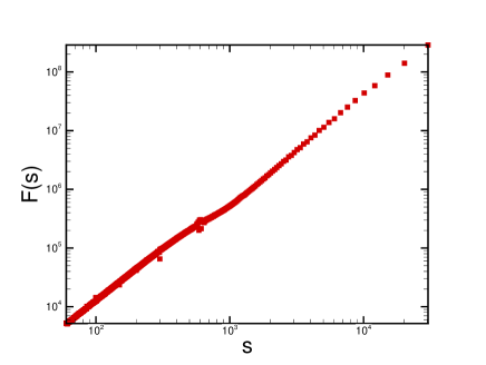
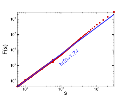
Figure 4: The log-log plot $F(s)$ versus $s$ for $q=2.0$ after double profiling for gray style, before F-DFA (Left) and After F-DFA (Right).

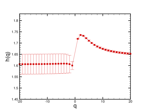
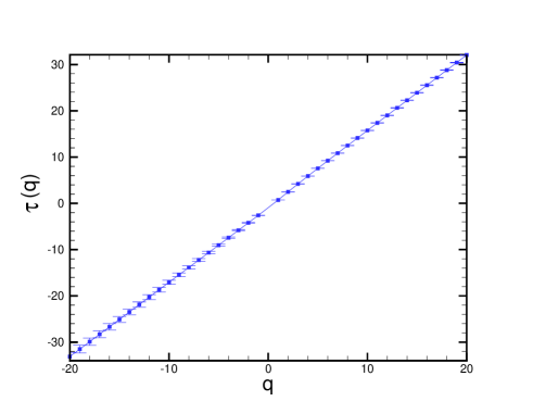
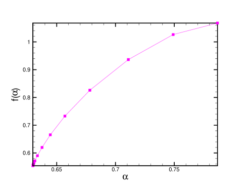
Figure 5: The q dependence of the exponents $h(q)$, $\tau(q)$ and singularity spectrum $f(\alpha)$, after double profiling, are shown in the upper to lower panels respectively for gray style.

2.1 Fourier-Detrended Fluctuation Analysis

In some cases, there exists one or more crossover length scales $s_{l}$ in graph $F(s)$, separating regimes with different scaling exponents [20]. In these cases, obtaining the scaling behavior is more complicated and different scaling exponents are required for different parts of the series [22]. Therefore, one needs a multitude of scaling exponents in various scales for a full description of scaling behavior. A crossover usually can arise from a change in correlation properties of the signal at different scales, or can often arise from trends in data. In addition, inappropriate detrending can create additional trends to signal which appear as crossovers in $F(s)$. The extra crossovers are not actual length scales of the original signal. In fact, these crossovers are due to the unsuitable detrending process. Fourier-Detrend Fluctuation Analysis (F-DFA) can be applied to remove crossovers such as sinusoidal trends. The F-DFA is a modified approach for the analysis of low frequency trends [39, 40, 41].

We transform data record to Fourier space in order to remove trends having a low frequency periodic behavior. Then we truncate the first few coefficients of the Fourier expansion and inverse Fourier transform of the series. After removing the sinusoidal trends we can obtain the fluctuation exponent using the direct calculation of the MF-DFA. If truncation numbers are sufficient, The crossovers due to sinusoidal trends in the log-log plot of $F_{q}(s)$ versus $s$ disappear.

3 Analysis of Color series

Most paintings are non-stationary due to the fact that all information is in whole of their structures. It means if we cut a part of a painting, we can not complete the remainder of it. Although there are some fractal paintings which all information is in each part of them. As mentioned in Sec. 2, a spurious of correlations may be detected using detrending methods in non-stationarity series. While, direct calculation of correlation behavior, spectral density exponent, fractal dimensions, etc., do not give us reliable results.

It seems that most of non-stationary properties in a painting are known trends such as objects. In fact, a painting consists of some objects or components have been set in various parts of it. As an example, a portrait has different parts such as eyes, nose, mouth, cheeks, eyebrows, etc. which can be considered as known trends. Also, light and shadow can be considered as trends. Since the art of painting is drawing the objects in an expressive manner, we intend to detrend data to characterize the artistic work of a painter regardless of the existence of specific objects (trends) in his or her paintings.

To construct color series, we need to relate a standard numerical quantity to each pixel. The basic colors are Red, Green and Blue (RGB), which every color is a specific combination of these basic colors. The standard value of each basic color is in the range of $0-255$. Therefore, we consider each color in our analysis and also we cover the gray style, which is a certain combination of these three basic colors. In the first step, it can be checked out that, all color series are non-stationary. One can verify non-stationarity property experimentally by measuring stability of their average and variance in a moving window for example using scale $s$. In fact, there are some specific lengths in painting that have important effects in statistical parameters. The picture’s width and height and color intensities are the first scaling parameters in painting. Moreover, the body and face detail structures are important scales that painter usually regards them. Let us determine whether the data set has a sinusoidal trend or not. According to MF-DFA1 method, Generalized Hurst exponents $h(q)$ in Eq. (4) can be found by analyzing log-log plots of $F_{q}(s)$ versus $s$ for each $q$ (Fig. 4). Our investigation shows that there is one crossover length scale $s_{l}$ in log-log plots of $F_{q}(s)$ versus $s$ for every $q$’s. To cancel the sinusoidal trends in MF-DFA1, we apply F-DFA method for color data. For eliminating the crossover scales, we need to remove only one term of the Fourier expansion. Then, by inverse Fourier Transformation, the noise without sinusoidal trend is extracted. Hurst exponent is between $0<H<1$. However, MF-DFA method can only determine positive generalized Hurst exponents, in order to refine the analysis near the fGn/fBm boundary or strongly anti-correlated signals when it is close to zero.

The simplest way to analyze such data is to integrate series before MF-DFA procedure. Hence, we replace the single summation in Eq. 1, which is describing the profile from the original data, by a double summation using signal summation conversion method (SSC) [38, 42, 43, 3]. After using SSC method, fGn switch to fBm and fBm switch to sum-fBm. In this case the relation between the new exponent, $h(q=2)$, and $H$ is $H=h(q=2)-1$ [38, 42, 43] (recently Movahed et al. have proven the relation between derived exponent from double profile of series in DFA method and $h(q=2)$ exponent in Ref. [42]). We find $h(q=2)=1.74\pm 0.01$ for gray style color series using SSC method. Therefore, Hurst exponent equals to $H=h(q=2)-1=0.74$.

The results of MF-DFA1 method for color signal are shown in Fig. 5, which show that these color series can be considered approximately as a monofractal process which is indicated by weak $q$ dependence of the exponents $h(q=2)$ and $\tau(q)$ [43]. The $q$ dependence of multifractal scaling exponent $\tau(q)$ approximately has a linear dependence to $q$ with equal slopes as $1.63$, $1.59$, $1.70$, and $1.66$ for gray, red, green, and blue styles, respectively. Table 1 shows the obtained quantities using MF-DFA1 method. Figure 5 shows the width of singularity spectrum ($f(\alpha)$) for gray style with $\Delta\alpha\simeq 0.15$ ($\Delta\alpha=\alpha(q_{max})-\alpha(q_{min})$). Its value indicates that the power of multifractality of the color series is weak [44].

Table 1: Values of $h(q=2)$, $\tau(q=2)$ exponents and width of singularity spectrum, $f(\alpha)$, $\Delta\alpha$ for $q=2.0$ of various styles obtained by MF-DFA1.

Style	$h(2)$	$\tau(2)$	$\Delta\alpha$
Gray	$1.74\pm 0.01$	$2.48\pm 0.01$	$0.15$
Red	$1.74\pm 0.01$	$2.48\pm 0.01$	$0.11$
Green	$1.72\pm 0.01$	$2.44\pm 0.01$	$0.12$
Blue	$1.74\pm 0.01$	$2.48\pm 0.01$	$0.12$

4 Conclusions

Using detrended methods for analyzing paintings, we can study the artistic manner of the painter, regardless of subject of the artworks. This is due to the fact that a painting consists of objects which can be considered as trends. The non-stationary property of paintings can be related to the objects, light and shadow, etc. Indeed by detrending methods, we eliminate trends from paintings and make the signal stationary. It means, we reduce the effects of objects, light and shadow, etc. from paintings. We have used multifractal detrended fluctuation analysis to detrend data to characterize the most famous artistic work of Leonardo da Vinci and shown the fractality of this painting. Our results using MF-DFA show that color series of Mona Lisa almost has the same behavior in various scales for all studied color styles (red, green, blue and gray).

References

- [1] R. P. Taylor, A. P. Micolich and D. Jonas Nature 399, 422 (1999).
- [2] W. Kandinsky, (1979) Point and line to plane, (New York, NY, Dover).
- [3] G. R. Jafari, P. Pedram, and L. Hedayatifar, J. Stat. Mech. P04012 (2007); G. R. Jafari, P. Pedram, K. Ghafoori Tabrizi, AIP Conf. Proc. 889, 310 (2007).
- [4] R. P. Taylor, R. Guzman, T. P. Martin, G. D. R. Hall, A. P. Micolich, D. Jonas, B. C. Scannell, M. S. Fairbanks, C.A. Marlow, Pattern Recognition Letters 28, 695 (2007).
- [5] L. Dagdug, J. Alvarez-Ramirez, C. Lopez, R. Moreno and E Hern, Physica A 383, 570 (2007).
- [6] M. Bigerelle, A. Iost, Chaos, Solitons and Fractals 11, 2179 (2000).
- [7] Z.-Y. Su, T. Wu, Physica D 221, 188 (2006).
- [8] Z.-Y. Su, T. Wu, Physica A 380, 418 (2007).
- [9] D. de Lima e Silvaa et al., Physica A 332, 559 (2004).
- [10] R. P. Taylor, New Scientist 159, 30 (1998).
- [11] R. P. Taylor et al., J. Non-lin. Dyn., Psych. Life Sci. 9, 89 (2005)
- [12] J. R. Mureika, Phys. Rev. E 72, 046101 (2005).
- [13] J. R. Mureika, Chaos 15, 043702 (2005).
- [14] J. R. Mureika, G. C. Cupchik, C. C. Dyer, Leonardo 37, 53 (2004).
- [15] C. K. Peng, S. V. Buldyrev, S. Havlin , M. Simons, H. E. Stanley, and A. L. Goldberger, Phys. Rev. E 49, 1685 (1994); S. M. Ossadnik, S. B. Buldyrev , A. L. Goldberger, S. Havlin, R. N. Mantegna, C. K. Peng, M. Simons and H. E. Stanley, Biophys. J. 67, 64 (1994).
- [16] H. E. Hurst , R. P. Black and Y. M. Simaika, (1965) Long-term storage. An experimental study (Constable, London).
- [17] J. F. Muzy, E. Bacry and A. Arneodo, Phys. Rev. Lett. 67, 3515 (1991).
- [18] M. Waechter, A. Kouzmitchev, J. Peinke, Phys. Rev. E 70, 055103 (2004). M. Vahabi, G. R. Jafari, Physica A 385, 583 (2007); F. Farahpour et al., Physica A 385, 601 (2007); F. Ghasemi et al., Phys. Rev. E 75, 060102 (2007).
- [19] M. S. Taqqu, V. Teverovsky, and W. Willinger, Fractals 3, 785 (1995).
- [20] J. W. Kantelhardt, E. Koscielny-Bunde, H. H. A. Rego, S. Havlin and A. Bunde, Physica A 295, 441 (2001).
- [21] K. Hu, P. Ch. Ivanov, Z. Chen, P. Carpena, and H. E. Stanley, Phys. Rev. E 64, 011114 (2001).
- [22] Z. Chen , P. Ch. Ivanov , K. Hu, and H. E. Stanley, Phys. Rev. E 65, 041107 (2002); P. Norouzzadeh, G. R. Jafari, Physica A 356 609 (2005).
- [23] S. V. Buldyrev, A. L. Goldberger, S. Havlin, R. N. Mantegna, M. E. Matsa, C. K. Peng, M. Simons, and H. E. Stanley, Phys. Rev. E 51, 5084 (1995); S. V. Buldyrev, N. V. Dokholyan, A. L. Goldberger, S. Havlin, C. K. Peng, H. E. Stanley, and G. M. Viswanathan, Physica A 249, 430 (1998).
- [24] P. Ch. Ivanov, A. Bunde, L. A. N. Amaral, S. Havlin, J. Fritsch-Yelle, R. M. Baevsky, H. E. Stanley, and A. L. Goldberger, Europhys. Lett. 48, 594 (1999); Y. Ashkenazy, M. Lewkowicz, J. Levitan, S. Havlin, K. Saermark, H. Moelgaard, P. E. B. Thomsen, M. Moller, U. Hintze, and H. V.Huikuri, Europhys. Lett. 53, 709 (2001); Y. Ashkenazy, P. Ch.Ivanov, S. Havlin, C. K. Peng, A. L. Goldberger, and H. E. Stanley, Phys. Rev. Lett. 86, 1900 (2001).
- [25] C. K. Peng, S. Havlin, H. E. Stanleyand, A. L. Goldberger, Chaos 5, 82 (1995).
- [26] A. Bunde, S. Havlin, J. W. Kantelhardt, T. Penzel, J. H. Peter and K. Voigt, Phys. Rev. Lett. 85, 3736 (2000).
- [27] R. N. Mantegna and H. E. Stanley, (2000) An Introduction to Econophysics (Cambridge University Press, Cambridge); Y. Liu, P. Gopikrishnan, P. Cizeau, M. Meyer, C. K. Peng, and H. E. Stanley, Phys. Rev. E 60, 1390 (1999); N. Vandewalle, M. Ausloos, and P. Boveroux, Physica A 269, 170 (1999).
- [28] K. Ivanova and M. Ausloos, Physica A 274, 349 (1999).
- [29] Z. Siwy, M. Ausloos, and K. Ivanova, Phys. Rev. E 65, 031907 (2002).
- [30] M. Ausloos and K. Ivanova, Phys. Rev. E 63, 047201 (2001).
- [31] M. Sadegh Movahed, Evalds Hermanis, Physica A 387, 915 (2008); G. R. Jafari, M. Sadegh Movahed, P. Noroozzadeh, A. Bahraminasab, Muhammad Sahimi, F. Ghasemi, M. Reza Rahimi Tabar, International Journal of Modern Physics C, 18, (2007) 1-9.
- [32] J. Feder, (1988) Fractals (Plenum Press, New York).
- [33] A. L. Barabási and T. Vicsek, Phys. Rev. A 44, 2730 (1991).
- [34] H. O. Peitgen, H. Jürgens and D. Saupe, (1992) Chaos and Fractals (Springer-Verlag, New York), Appendix B.
- [35] E. Bacry, J. Delour and J. F. Muzy, Phys. Rev. E 64, 026103 (2001).
- [36] U. Fano, Phys. Rev. 72, 26 (1947).
- [37] J. A. Barmesand D. W. Allan, Proc. IEEE 54, 176 (1996).
- [38] A. Eke, P. Herman, L. Kocsis and L. R. Kozak, Physiol. Meas. 23, R1-R38 (2002).
- [39] R. Nagarajan and R. G. Kavasseri, Int. Journal of Bifurcations and Chaos 15, 1767 (2005).
- [40] C. V. Chianca, A. Ticona, and T. J. P. Penna, Physica A 357, 447 (2005).
- [41] E. Koscielny-Bunde, A. Bunde, S. Havlin, H. E. Roman, Y. Goldreich, and H. J. Schellnhuber, Phys. Rev. Lett. 81, 729 (1998).
- [42] M. Sadegh Movahed, G. R. Jafari, F. Ghasemi , S. Rahvar, and M. Reza Rahimi Tabar, J. Stat. Mech. P02003 (2006).
- [43] J. W. Kantelhardt, S. A. Zschiegner, E. Kosciliny-Bunde, A. Bunde, S. Pavlin, and H. E. Stanley, Physica A 316, 78 (2002).
- [44] P. Oswiecimka, J. Kwapien, S. Drozdz, Phys. Rev. E 74, 016103 (2006).