Transport in anisotropic model systems analyzed by a correlated projection superoperator technique

Abstract

By using a correlated projection operator, the time-convolutionless (TCL) method to derive a quantum master equation can be utilized to investigate the transport behavior of quantum systems as well. Here, we analyze a three-dimensional anisotropic quantum model system according to this technique. The system consists of Heisenberg coupled two-level systems in one direction and weak random interactions in all other ones. Depending on the partition chosen, we obtain ballistic behavior along the chains and normal transport in the perpendicular direction. These results are perfectly confirmed by the numerical solution of the full time-dependent Schrödinger equation.

I Introduction

The transport of different extensive quantities like energy, heat, entropy, mass, charge, magnetization, etc., through and within solid state systems is an intensively studied topic of nonequilibrium statistical dynamics. Nevertheless, there are numerous open questions concerning the type of transport especially in small systems far from the thermodynamic limit and in particular in quantum mechanics. At the heart of many investigations is the classification into two main categories: normal or diffusive transfer of the extensive quantity and ballistic transport featuring a divergence of the conductivity.

Diffusive transport occurs whenever the system is governed by a diffusion equation. In particular, this means that excitations decay exponentially fast and the spatial variance of an initial excitation grows linear in time. Ballistic transport, however, is rather described by the equations of motion of a free particle. For the spatial variance of an excitation this implies a quadratic growth in time.

In the present paper, we will concentrate on the transport of energy and heat in quantum systems. There are several different approaches discussed in the literature to investigate the transport of those quantities in quantum mechanics. One very famous ansatz is the investigation of heat transport in terms of the Green-Kubo formula Zotos et al. (1997); Prosen (1999); Klümper and Sakai (2002); Heidrich-Meisner et al. (2003); Saito (2003a); Jung et al. (2006). A main advantage of this approach is certainly its computability after having diagonalized the system’s Hamiltonian. Derived on the basis of linear response theory the Kubo formula has originally been formulated for electrical transport Kubo (1957); Kubo et al. (1991), where an external potential can be written as an addend to the Hamiltonian of the system. Basically one finds a current-current autocorrelation, which has ad hoc been transferred to heat transport simply by replacing the electrical current by a heat current Luttinger (1964). However, the justification of this replacement remains unclear since there is no way of expressing a temperature gradient in terms of an addend to the Hamiltonian of the system as before Gemmer et al. (2006).

Other approaches to heat conductivity in quantum systems are based on diagonalization of the Schrödinger equation Gobert et al. (2005), analyzing the level statistics of the Hamiltonian Mejía-Monasterio et al. (2005); Steinigeweg et al. (2006) or by an explicit coupling to some environments of different temperature Saito (2003b); Michel et al. (2003). In the latter case, environments are described by a quantum master equation Breuer and Petruccione (2002) in Liouville space. Here the temperature differences can, indeed, be described by a perturbation operator so that one may treat a thermal perturbation in this extended state space similar as an electrical one in the Hilbert space Michel et al. (2004).

The Hilbert space Average Method Gemmer et al. (2004) allows for a direct investigation of the heat transport in quantum systems from Schrödinger dynamics. By deriving a reduced dynamical equation for a class of design quantum systems, normal heat transport as well as Fourier’s Law has been confirmed Michel et al. (2005, 2006). Recently, it has been shown that for diffusive systems the Hilbert space average method is equivalent to a projection operator technique with an extended projection superoperator Breuer et al. (2006); Breuer (2007). However, ballistic behavior cannot be analyzed with the Hilbert space Average Method in a straightforward manner since it is not obvious how to obtain time-dependent rates.

Using a correlated superprojection operator within the derivation of the time-convolutionless (TCL) quantum master equation leads to a reduced dynamical description of the investigated system. The main advantage of the correlated TCL method refers to its perturbation theoretical character. Thus it is a systematic expansion in some perturbational parameter.

To use this alternative method for an investigation of the transport behavior of a quantum system, it is necessary to partition the microscopic system described by the Hamiltonian $\hat{H}$ into mesoscopic subunits. While the complete dynamics is governed by the Schrödinger equation of the full system according to its density operator

$$\dot{\hat{\rho}}=-\frac{i}{\hbar}[\hat{H},\hat{\rho}]\equiv\mathcal{L}(t)\hat{\rho},$$ (1)

we aim at deriving a closed reduced dynamical equation for the subunits chosen. Formally, this partitioning is done by introducing a projection superoperator $\mathcal{P}$ that projects onto the relevant part of the full density matrix $\hat{\rho}$ Breuer and Petruccione (2002), here the spatial energy distribution within the system. However, by a straightforward application of the projection superoperator on the above equation, the dynamics of the reduced system is no longer unitary, but described by

$$\mathcal{P}\dot{\hat{\rho}}=\mathcal{P}\mathcal{L}(t)\hat{\rho}.$$ (2)

These effective equations of motion for the relevant part $\mathcal{P}\hat{\rho}$ can either be written as an integro-differential equation (Nakajima-Zwanzig equation Nakajima (1958); Zwanzig (1960)) or as a time-convolutionless (TCL) master equation Breuer and Petruccione (2002), which is an ordinary linear differential equation of first order. Both methods allow for a systematic perturbative expansion. In the TCL expansion series the first-order term typically vanishes and thus the leading order is given by (cf. Breuer et al. (2006); Breuer (2007))

$$\mathcal{P}\dot{\hat{\rho}}=-\int\limits_{0}^{t}dt_{1}\mathcal{P}\mathcal{L}(t)\mathcal{L}(t_{1})\mathcal{P}\hat{\rho}.$$ (3)

However, in order to obtain a converging perturbation series expansion $\mathcal{P}$ should not be chosen arbitrarily: A “wrong” projection superoperator may lead to a breakdown of the expansion Breuer et al. (2006).

II Description of the model

In the present paper we consider a three-dimensional (3D) model composed of two-level systems. The coupling between the atoms is anisotropic, i.e., in one direction dominated by a Heisenberg interaction whereas the coupling in all other directions is random. The choice of random couplings ensures that the interaction is unbiased as it does not have any special symmetry. Two-level atoms or spin-$1/2$ systems Schollwöck et al. (2004) allow to study a large variety of quantum effects from quantum information processing to solid state theory, described by a rather simple interaction, making them interesting both from an experimental and theoretical point of view. Of particular interest are the transport properties of systems containing 1D and 2D spin structures, e.g., the investigations of heat transport in cuprates, in which a dramatic heat transport anisotropy has been reported Sologubenko et al. (2000); Hess et al. (2001). While the anisotropy is mainly attributed to anisotropic phonon scattering processes, we investigate transport anisotropies emerging from an anisotropic (but coherent) interaction.

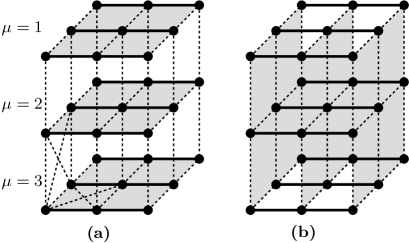
Figure 1: Partition schemes for investigating the transport perpendicular (a) or parallel (b) to the spin chains. Each spin is represented by a dot, solid lines indicate Heisenberg interactions along the chains, dashed lines represent random interactions. The diagonal couplings within each plane have been left out for clarity [except the lower left corner of (a)].

The model we are going to investigate is a three-dimensional model of two-level systems depicted in Fig. 1. In terms of Pauli operators the local Hamiltonian of the network is given by

$$\hat{H}_{loc}=\frac{\Delta E}{2}\sum\limits_{i}\hat{\sigma}_{z}^{(i)},$$ (4)

with the local energy splitting $\Delta E$ defining the basic energy unit within our model.

In $x$ direction, the two-level systems are coupled via a Heisenberg interaction

$$\hat{H}_{H}=\sum\limits_{i}\hat{\bm{\sigma}}^{(i)}\otimes\hat{\bm{\sigma}}^{(i+1)},$$ (5)

with the Pauli spin vectors $\hat{\bm{\sigma}}^{(i)}=(\hat{\sigma}_{x}^{(i)},\hat{\sigma}_{y}^{(i)},\hat{\sigma}_{z}^{(i)})$ at site $i$.

In the $y$ and $z$ directions, we use a random interaction matrix $\hat{H}_{R}$ to couple both adjacent sites and next neighbor sites lying diagonally opposite [see lower left corner of Fig. 1(a)]. The nonzero matrix elements are taken from a Gaussian ensemble with zero mean and a variance $s^{2}$. While each matrix element is taken from the same ensemble, the geometry of the system requires that we do not have translational invariance within the random interaction.

To investigate the transport in $x$ or $z$ direction, respectively (cf. Fig. 1), we perform a partition of the model into $N$ subunits. A layer of $n$ two-level systems is grouped together into a new local subsystem, coupled to adjacent layers by the connections between pairs of two level systems. Because of the anisotropy within the model we can study the transport perpendicular to the Heisenberg chains in the $z$ direction [Fig. 1(a)] and along the chains in $x$ direction [Fig. 1(b)].

The coupling strength of an arbitrary interaction matrix $\hat{V}$ is defined as

$$\eta=\frac{1}{d}\sqrt{\text{Tr}\{\hat{V}^{\dagger}\hat{V}\}},$$ (6)

with $d$ being the dimension of the matrix (see Gemmer et al. (2004)). For the random interaction we choose the variance $s^{2}$ in such a way that $\eta=1$ for all interaction matrices coupling adjacent subunits.

The complete Hamiltonian of the full model system is thus described by

$$\hat{H}=\hat{H}_{loc}+\lambda_{H}\hat{H}_{H}+\lambda_{R}\hat{H}_{R}.$$ (7)

Because of the normalization of the interaction matrices the numbers $\lambda_{H}$ and $\lambda_{R}$ define the coupling strength between different sites. The coupling strengths $\lambda_{H}$ for the Heisenberg interaction and $\lambda_{R}$ for the random interaction are chosen so that $\lambda_{R}\ll\lambda_{H}\ll\Delta E$, which is known as the weak coupling limit.

Regardless of the partition scheme chosen (in the $x$ or $z$ direction) each subunit can be seen as a molecule consisting of several energy bands. However, the solution for the complete system is computationally unfeasible for more than a few sites. If we restrict ourselves to initial states where only one site is excited (or superpositions thereof) the Heisenberg interaction does not allow to leave this subspace of the total Hilbert space. By choosing also the random interaction to conserve this subspace we restrict all further investigations to the single excitation subspace. Figure 2 gives a graphical representation of our system, with $\delta\varepsilon$ being the width of the first energy band (all higher excitation bands are neglected here).

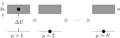
Figure 2: $N$ subunits with ground state and first excitation band of width $\delta\varepsilon$ containing $n$ energy levels each. Black dots specify the initial states used.

Interpreting our model system in terms of a magnetic system, i.e., the two-level atoms representing coupled spins in a magnetic field for example, the considered energy transport is equivalent to spin transport in a gapless system (i.e. $\Delta E=0$).

III Transport in the $\bm{z}$ direction

III.1 Partitioning scheme

Let us consider the transport perpendicular to the Heisenberg chains (in the $z$ direction) first. Then, the partitioning into subunits yields the following mesoscopic Hamiltonian consisting of a local and an interaction part

$$\hat{H} =\hat{H}_{L}+\hat{H}_{I}$$

$$=\sum_{\mu=1}^{N}\hat{H}_{L}(\mu)+\sum_{\mu=1}^{N-1}\hat{H}_{I}(\mu,\mu+1).$$ (8)

Here $\hat{H}_{L}(\mu)$ of subunit $\mu$ consists of the constant local energy splitting, the Heisenberg interaction, and the internal random couplings of each subunit [cf. gray planes in Fig 1(a)]. Since $\lambda_{R}\ll\lambda_{H}$ the effect of the internal random couplings on the spectrum of $\hat{H}_{L}(\mu)$ may be neglected. Therefore the bandwidth $\delta\varepsilon$ is determined by the Heisenberg interaction given by

$$\delta\varepsilon=8\lambda_{H}.$$ (9)

The last term in Eq. (III.1), $\hat{H}_{I}(\mu,\mu+1)$, denotes the interaction between the subunits which is purely random here, i.e., contains parts of the random interaction Hamiltonian $\hat{H}_{R}$ only.

III.2 Derivation of the TCL master equation

The correlated projection superoperator $\mathcal{P}$ introduced in Sec. I is of the type as suggested by Breuer Breuer (2007) and reads

$$\mathcal{P}\hat{\rho}=\sum_{\mu}\text{Tr}\{\hat{\Pi}_{\mu}\hat{\rho}\}{}\frac{1}{n}\hat{\Pi}_{\mu}\equiv\sum_{\mu}P_{\mu}\frac{1}{n}\hat{\Pi}_{\mu},$$ (10)

with $\hat{\Pi}_{\mu}$ being the standard projection operators

$$\hat{\Pi}_{\mu}=\sum_{n_{\mu}}\mathopen{|}n_{\mu}\mathclose{\rangle}\mathopen{\langle}n_{\mu}\mathclose{|},$$ (11)

and $\mathopen{|}n_{\mu}\mathclose{\rangle}$ the eigenstate of $\hat{H}_{L}(\mu)$ in the one-particle excitation subspace, i.e. the states in the band of subunit $\mu$ (cf. Fig. 2). Consequently, the number $P_{\mu}$ is just the excitation probability of subunit $\mu$. This choice of $\mathcal{P}$ thus implements the partitioning scheme required for studying transport behavior.

Switching to the interaction picture, plugging both the Hamiltonian (III.1) and the projection (10) into Eq. (3) we get

$$\dot{P}_{\mu}=-\frac{\lambda_{R}^{2}}{n\hbar^{2}}\sum_{\nu}\int_{0}^{t}dt_{1}\text{Tr}\{\hat{\Pi}_{\mu}[\hat{H}_{R}(t),[\hat{H}_{R}(t_{1}),\hat{\Pi}_{\nu}]]\}{}P_{\nu}$$ (12)

for the second order TCL expansion. The time dependencies of the coupling operators refer to the transformation into the interaction picture and are defined as

$$\hat{H}_{R}(t)=e^{i\hat{H}_{L}t}\,\hat{H}_{R}\,e^{-i\hat{H}_{L}t}.$$ (13)

By exploiting that $\hat{\Pi}_{\mu}$ projects onto eigenstates of $\hat{H}_{L}(\mu)$ we can evaluate the trace by using the block structure of the interaction $\hat{H}_{I}(\mu,\mu+1)$ between adjacent subunits (see Michel et al. (2005, 2006)), resulting in

$$\frac{d{P}_{\mu}}{dt}=-\gamma_{\mu}\big{(}2P_{\mu}-P_{\mu+1}-P_{\mu-1}\big{)}$$ (14)

with the decay rate

$$\gamma_{\mu}=\frac{2\lambda_{R}^{2}}{n\hbar^{2}}\sum_{k,l}^{n}|\mathopen{\langle}k_{\mu}\mathclose{|}\hat{H}_{R}\mathopen{|}l_{\mu+1}\mathclose{\rangle}|^{2}\,\frac{\sin(\omega_{kl}t)}{\omega_{kl}}.$$ (15)

The frequency $\omega_{kl}$ refers to the transition between the eigenstates $k$, $l$. Equation (14) is basically a rate equation for the probabilities to find an excitation in subunit $\mu$.

III.3 Decay rate

Since the interaction between two adjacent subunits is a random matrix with the above described properties, all matrix elements are approximately of the same size. That means that the rate does not depend on the subunit $\mu$ ($\gamma_{\mu}=\gamma$). Furthermore, we can assume $|\mathopen{\langle}k_{\mu}\mathclose{|}\hat{H}_{R}\mathopen{|}l_{\mu+1}\mathclose{\rangle}|^{2}\approx 1$, finding

$$\gamma=\frac{2\lambda_{R}^{2}}{n\hbar^{2}}\sum_{k,l}\frac{\sin\omega_{kl}t}{\omega_{kl}}.$$ (16)

In the following the double sum is treated analogous to the derivation of Fermi’s Golden Rule.

Since the sine cardinal (sinc) of Eq. (16) is a representation of the Dirac $\delta$-distribution

$$\pi\delta_{t}(\omega_{kl})=\lim_{t\rightarrow\infty}\frac{\sin(\omega_{kl}t)}{\omega_{kl}},$$ (17)

we may approximate the rate for not too small $t$ by

$$\gamma \approx\frac{2\pi\lambda_{R}^{2}}{n\hbar}\sum_{k,l}\delta(E_{k}-E_{l}).$$ (18)

Replacing the double sum over integrals in the energy space we arrive at

$$\gamma\approx\frac{2\pi\lambda_{R}^{2}}{n\hbar}\int_{0}^{\delta\varepsilon}g^{2}(E)\,dE$$ (19)

with the state density $g(E)$, i.e., the integral over the square of the density of states. Since we have neglected the internal random interaction completely, the state density of the first excitation subspace is just given by the state density of a Heisenberg spin chain

$$g(E)=\frac{2n}{\pi\delta\varepsilon}\frac{1}{\sqrt{1-\left(\frac{2E}{\delta\varepsilon}-1\right)^{2}}}.$$ (20)

Unfortunately, this function is not square integrable due to singularities at the boundaries of the spectrum. However, due to symmetry we have

$$\int_{0}^{\delta\varepsilon}g^{2}(E)\,dE=2\int_{0}^{\delta\varepsilon/2}g^{2}(E)\,dE.$$ (21)

In order to avoid the singularity at $E=0$ we renormalize the number of states in the band. We introduce the regularized integral

$$F_{\Lambda}(n) =2\int_{\Lambda}^{\delta\varepsilon/2}\alpha^{2}g^{2}(E)\,dE$$

$$=2\int_{\Lambda}^{\delta\varepsilon/2}\frac{\alpha^{2}n^{2}}{\pi^{2}E(\delta\varepsilon-E)}\,dE,$$ (22)

with $\alpha$ being the factor that renormalizes the number of states. We assume that for a band consisting of only a few levels $\tilde{n}$ (but still enough to define a density of states), the density of states is approximately constant. For a constant density of states $\tilde{g}(E)$ we simply have

$$2\int_{0}^{\delta\varepsilon/2}\tilde{g}^{2}(E)\,dE=\frac{\tilde{n}^{2}}{\delta\varepsilon},$$ (23)

therefore our renormalization prescription is given by

$$F_{\Lambda}(\tilde{n})=\frac{\tilde{n}^{2}}{\delta\varepsilon}.$$ (24)

Using this result to solve Eq. (III.3) for $\alpha$ at constant $\tilde{n}$ yields

$$\alpha=\frac{\pi}{\sqrt{2\ln(\delta\varepsilon/\Lambda-1)}}.$$ (25)

This allows us to calculate the physical limit of the renormalization procedure, i.e.,

$$\lim\limits_{\Lambda\rightarrow 0}F_{\Lambda}(n)=\frac{n^{2}}{\delta\varepsilon}$$ (26)

which is the same value as for a constant density of states. This finally leads to the relaxation rate

$$\gamma=\frac{2\pi\lambda_{R}^{2}n}{\hbar\delta\varepsilon}.$$ (27)

The approximation introduced by Fermi’s Golden Rule is only valid in the linear regime (see Gemmer et al. (2004)), i.e.,

$$\frac{4\pi^{2}n\lambda_{R}^{2}}{\delta\varepsilon^{2}}\ll 1.$$ (28)

III.4 Solution of the TCL master equation

Figure 3 shows both the numerical results for the solution of the full Schrödinger equation and the solution of the rate equation (14), according to the above derived approximation for the rate $\gamma$ [cf. Eq. (27)]. Both are in reasonably good agreement.

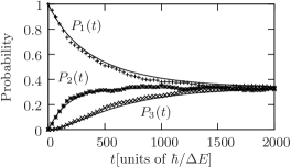
Figure 3: Perpendicular transport: probability to find the excitation in subunit $\mu=1,2,3$. Comparison of the numerical solution of the Schrödinger equation (crosses) and second-order TCL (lines). ($N=3$, $n=600$, $\lambda_{R}=5\cdot 10^{-4}\Delta E$, $\lambda_{H}=6.25\cdot 10^{-2}\Delta E$)

Equation (14) is a discrete version of the diffusion equation, which does not change when regarding the thermodynamic limit ($n,N\rightarrow\infty$, $n\lambda_{R}^{2}=\textup{const}$). For a $\delta$-shaped excitation at $t=0$ its solution is a Gaussian function, the variance of which grows linear in time. Therefore, it is evident that the heat transport is normal perpendicular to the chains.

IV Transport in the $\bm{x}$ direction

IV.1 Partitioning scheme

In the following let us concentrate on the transport in the $x$ direction, i.e., parallel to the chains. Thus, we have a slightly different partition of the total Hamiltonian. Besides the local energy splitting, the local part $\hat{H}_{L}$ of the mesoscopic Hamiltonian (III.1) contains random interactions only:

$$\hat{H}_{L}=\sum_{\mu=1}^{N}\big{[}\hat{H}_{loc}(\mu)+\lambda_{R}\hat{H}_{R}(\mu)\big{]}.$$ (29)

In contrast, the interaction between the subunits consists of a Heisenberg and a random part,

$$\hat{H}_{I}=\sum_{\mu=1}^{N-1}\big{[}\lambda_{H}\hat{H}_{H}(\mu,\mu+1)+\lambda_{R}\hat{H}_{R}(\mu,\mu+1)\big{]}.$$ (30)

In the one-particle excitation subspace the commutator relations

$$[\hat{H}_{H},\hat{H}_{L}]=[\hat{H}_{H},\hat{H}_{R}]=0$$ (31)

are satisfied. If the dynamics induced by the local part $\hat{H}_{L}$ and the Heisenberg $\hat{H}_{H}$ is absorbed in the transformation into the interaction picture, the random part of the interaction transforms into

$$\hat{H}_{R}(t) =e^{i\left(\hat{H}_{H}+\hat{H}_{L}\right)t}\,\hat{H}_{R}\,e^{-i\left(\hat{H}_{H}+\hat{H}_{L}\right)t}$$

$$=e^{i\hat{H}_{L}t}\,\hat{H}_{R}\,e^{-i\hat{H}_{L}t},$$ (32)

where Eq. (31) has been used. Note that this is not the standard interaction picture as used above, but a special one allowing us to treat the transport in the $x$ direction in a similar manner as in the $z$ direction. According to this transformation the derivation of the second order TCL master equation in Sec. III.2, especially Eqs. (12), (14) and (15), remain unchanged.

IV.2 Decay rate

However, the computation of the rate (16) is different here. For calculating the local band structure we consider just a random matrix of dimension $n$, drawn from a Gaussian unitary ensemble. From random matrix theory Mehta (1991) it is known that the density of levels $\zeta(x)$ for such a random Hermitian matrix consisting of elements with zero mean and unit variance for both real and imaginary parts is given by

$$\zeta(x)=\frac{1}{\pi}\sqrt{2n-x^{2}}.$$ (33)

Mapping this to a density of energy levels leads to

$$g(E)=\frac{8n}{\pi\delta\varepsilon}\sqrt{\frac{\delta\varepsilon^{2}}{4}-E^{2}}.$$ (34)

We rescale the variance to the interaction strength $\lambda_{R}$, which gives for the bandwidth

$$\delta\varepsilon=4\sqrt{n}\lambda_{R}.$$ (35)

In order to check whether our local Hamiltonian $\hat{H}_{L}$ can be approximated by such a random matrix, we compare the eigenvalues $E(x)$ of both matrices. Using

$$\frac{dE}{dx}=\frac{1}{g[E(x)]}$$ (36)

and separating variables yields

$$\frac{8n}{\pi\delta\varepsilon}\sqrt{\frac{\delta\varepsilon^{2}}{4}-E^{2}}\,dE=dx,$$ (37)

with the state density (34). This expression cannot be solved analytically for $E$, so we compare the numerical solution for discrete values of $x$ with the eigenvalues of $\hat{H}_{L}$. As Fig. 4 shows, $\hat{H}_{L}$ may indeed be approximated by a random matrix drawn from a Gaussian unitary ensemble. However, by plugging Eq. (35) into Eq. (28) one gets a constant value of $\pi^{2}/4$ which is definitely not small compared to one. Thus, the requirement for the linear regime is violated and the derivation of the rate according to Fermi’s Golden Rule can no longer be applied.

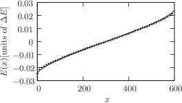
Figure 4: Comparison of the eigenvalues of $\hat{H}_{L}$ and a random matrix drawn from a Gaussian unitary ensemble. ($n=600$, $\lambda_{R}=5\cdot 10^{-4}\Delta E$)

The approximation used in Sec. III.2 is analogous to Fermi’s Golden Rule. All transitions in Eq. (16) from $l$ to $k$ are weighted by the respective value of the sinc function which changes its shape for increasing times to approach a delta peak for $t\rightarrow\infty$. In the situation described above the decay takes place within the linear regime, i.e., at an intermediate time scale. That means that all possible transition frequencies are distributed below the peak. Thus the sum in Eq. (16) can be approximated by the area under the peak (see Gemmer et al. (2004)).

This is not the case here. The decay happens on a much shorter time scale, when the peak is extremely broad. Therefore almost any transition frequency belongs to the maximum of the peak. Thus the sinc in Eq. (16) should better be approximated by the maximum value of the peak, instead of the area under the peak. The maximum value grows with time according to $t$. Thus the double sum over sinc functions could be approximated by $n^{2}t$. This means that we get the relaxation rate

$$\gamma=\frac{2n\lambda_{R}^{2}}{\hbar^{2}}\,t.$$ (38)

IV.3 Solution of the TCL master equation

The solution of Eq. (14) with the diffusion coefficient (38) defines the occupation probabilities in the interaction picture $P_{\mu}^{\textup{int}}$. Note that in the other direction the occupation probabilities of the interaction picture have been equivalent to the occupation probabilities in the Schrödinger picture. This is not the case for the present situation because of the special choice of the interaction picture. Remember that we have used not only the local Hamiltonian for the transformation into the interaction picture, but also a part of the inter-subsystem interaction [cf. Eq. (IV.1)].

Since we are interested in the occupation probabilities in the Schrödinger picture $P_{\mu}^{\textup{s}}$ we need to calculate the inverse transformation of the density operator

$$\mathcal{P}\hat{\rho}^{\textup{s}}=e^{-i\hat{H}_{H}t}\mathcal{P}\hat{\rho}^{\textup{int}}e^{i\hat{H}_{H}t},$$ (39)

where the diagonal elements $\mathcal{P}\hat{\rho}^{\textup{s}}_{\mu\mu}$ are the occupation probabilities $P_{\mu}^{\textup{s}}$. The off-diagonal elements of $\mathcal{P}\hat{\rho}^{\textup{int}}$ can be computed by replacing the projector (11) with another one projecting out off-diagonal elements as well. The dynamics of the diagonal and the off-diagonal elements decouple so that diagonal initial states remain diagonal for all time.

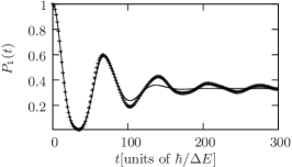
Figure 5: Parallel transport: probability to find the excitation in the first subunit ($\mu=1$). Comparison of the numerical solution of the Schrödinger equation (crosses) and second-order TCL (solid line). (Same parameters as for Fig. 3)

Thus using Eq. (39) for the inverse transformation we get the time-dependent solution of the probabilities in the Schrödinger picture. In Fig. 5 the numerical solution of the Schrödinger equation is compared with the TCL prediction. Again, there is a very good agreement between the exact solution and our second order approximation.

IV.4 Spatial variance

To classify the transport behavior in the $x$ direction a very large system has to be considered, so that the initial excitation does not reach the boundaries of the system during the relaxation time. Since the solution of the time-dependent Schrödinger equation becomes unfeasible the second-order TCL prediction has been used for subsequent numerical integration. The variance of an excitation initially at $\mu=\mu_{0}$,

$$\sigma^{2}(t)=\sum\limits_{\mu=1}^{N}P_{\mu}^{(s)}(t)(\mu-\mu_{0})^{2},$$ (40)

shown in Fig. 6 grows quadratic in time, i.e., the transport is ballistic. Here we have considered a system with $N=300$ subunits and an initial excitation at $\mu_{0}=150$ solving the TCL master equation. This is also valid in the thermodynamic limit as $\gamma(t)$ does not change. Numerical investigations show that the transport behavior is largely independent of $\gamma(t)$. Ballistic transport is observed as long as $\lambda_{H}t\gg\gamma(t)$ on all relevant time-scales.

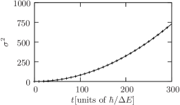
Figure 6: Variance of an excitation initially at subunit $\mu_{0}=150$. Second-order TCL prediction (crosses) and quadratic fit (solid line). ($N=300$, $n=600$, $\lambda_{R}=5\cdot 10^{-4}$, $\lambda_{H}~{}=~{}6.25~{}\cdot~{}10^{-2}$)

V Conclusions

In the present paper we have demonstrated how the abstract method of correlated projection superoperators for the TCL master equation Breuer et al. (2006); Breuer (2007) can be used to analyze the transport behavior of a three-dimensional solid state model: a system of coupled two-level atoms with an anisotropic interaction. The analysis is based on the following preconditions:

1. a partitioning scheme in position space to consider the transport in one direction of the model, thus introducing a projection superoperator

2. the convergence of the TCL expansion in second order (a wrong projection superoperator leads to a diverging expansion, or large higher than second orders)

3. an approximation scheme for computing the decay rate to avoid numerical integration

According to those central points a reduced dynamical description of the complex quantum model is derived which can be analyzed, e.g., to classify the transport behavior of the system.

By a comparison of the TCL prediction with the exact numerical solution of the complete Schrödinger equation of our model system we have shown that the results of the method are in very good accordance with the real dynamical behavior of the system. Having established a method which efficiently describes the dynamical properties of a complex quantum model the transport behavior can be classified by either an analytic analysis of the solution of the reduced dynamical equations or by a numerical investigation. Here, the simplicity of the reduced equations in comparison to the exact system of differential equations allows us to investigate the dynamical properties of a much larger system which is not accessible to a direct investigation.

The analysis shows that the model features two very different types of transport behavior in the $x$ and $z$ directions, perpendicular or parallel to the chains, respectively. In the $z$ direction we have found a standard statistical decay behavior following a diffusion equation on the basis of the mesoscopic subunits. In this way diffusive behavior has been derived from first principles on a mesoscopic scale whereas the dynamics on the microscopic scale (i.e., of a single spin) is obviously non-diffusive. This indicates that the transport behavior is not only a property of a system per se, but also depends on the way we are looking at it. In contrast the model shows ballistic behavior parallel to the chains which is demonstrated by the features of the reduced dynamical equations. Note that this behavior is similar to investigations of large anisotropies within the heat conductivity of cuprates Sologubenko et al. (2000); Hess et al. (2001).

In conclusion this method of a correlated projection superoperators within TCL allows to investigate the dynamical behavior of 3D model systems on a mesoscopic scale. It is useful both in the case of a statistical decay according to a diffusion equation and the ballistic case, where time dependent rates are important.