The DEEP2 Galaxy Redshift Survey: The Red Sequence AGN Fraction and its Environment and Redshift Dependence

Abstract

We measure the dependence of the AGN fraction on local environment at $z\sim 1$, using spectroscopic data taken from the DEEP2 Galaxy Redshift Survey, and Chandra X-ray data from the All-Wavelength Extended Groth Strip International Survey (AEGIS). To provide a clean sample of AGN we restrict our analysis to the red sequence population; this also reduces additional colour–environment correlations. We find evidence that high redshift LINERs in DEEP2 tend to favour higher density environments relative to the red population from which they are drawn. In contrast, Seyferts and X-ray selected AGN at $z\sim 1$ show little (or no) environmental dependencies within the same underlying population. We compare these results with a sample of local AGN drawn from the SDSS. Contrary to the high redshift behaviour, we find that both LINERs and Seyferts in the SDSS show a slowly declining red sequence AGN fraction towards high density environments. Interestingly, at $z\sim 1$ red sequence Seyferts and LINERs are approximately equally abundant. By $z\sim 0$, however, the red Seyfert population has declined relative to the LINER population by over a factor of $7$. We speculate on possible interpretations of our results.

1 Introduction

Both active galactic nuclei (AGN) and local environment play key roles in shaping galaxy evolution. It is now understood that AGN are those nuclei in galaxies that emit radiation powered by accretion onto a supermassive black hole. Although this realisation has proved useful for explaining many observed characteristics of these active objects, there are still many unsolved problems, especially related to the physics of the accretion process itself. In the recent years much effort has been invested in studying the global properties of AGN as a unique population in the context of galaxy formation. In this work, we focus on a fundamental question: the dependence of the fraction of galaxies that have AGN on the density of the local environment at $z\sim 1$, and the evolution of this dependence to $z\sim 0$.

At low redshift, many authors have investigated various correlations between galaxy properties and environment. It is now well established that there exists a relationship between morphology and density (Oemler 1974 and Dressler 1980), in that star-forming disk-dominated galaxies tend to inhabit less dense regions of the Universe than “quiescent” or inactive elliptical galaxies. Moreover, additional (and related) dependencies with environment have been found, such as with stellar mass, luminosity, colour, recent and past star formation, star formation quenching, surface brightness, and concentration (to name but a few) (e.g. Kauffmann et al., 2004; Balogh et al., 2004; Hogg et al., 2004; Blanton et al., 2005; Bundy et al., 2006).

In this scenario of entangled correlations it is useful to investigate the dependence of AGN properties on the local environment, especially since AGN are believed to play an important part in shaping galaxy evolution. This has sometimes been a rather controversial issue. In the local Universe, Miller et al. (2003) found no dependence on environment of the fraction of spectroscopically selected AGN, using the SDSS early data release. This result is in good agreement with Sorrentino et al. (2006) who used the much larger SDSS DR4. However, many other authors claim the existence of a strong link between nuclear activity and environment, at least for specific AGN types. Kauffmann et al. (2004) found that intermediate luminosity optically selected AGN (Seyfert IIs) favoured underdense environments, while low-luminosity optically selected AGN (Low-Ionization Nuclear Emission-line Regions; hereafter, LINERs) showed no density dependence, within the SDSS DR1. Similarly, lower-luminosity AGN were found to have a higher clustering amplitude than high-luminosity AGN by Wake et al. (2004) and Constantin & Vogeley (2006). Radio-loud AGN have been noted to reside preferentially in mid-to-high density regions and tend to avoid underdense environments (Zirbel, 1997; Best, 2004).

At high redshift the study of both galaxies and AGN, and their relation to the environment, has been restricted by the lack of adequate data. Only in recent years, with the emergence of quality large-scale probes of the high redshift galaxy population, such as the DEEP2 Galaxy Redshift Survey (Davis et al., 2003) or the VIMOS-VLT Deep Survey (VVDS, Le Fevre et al., 2003), have we reached the stage where we can begin to measure the statistics of galaxy evolution in some detail. Using DEEP2, Cooper et al. (2006) found that the many of the low redshift galaxy correlations with environment are already in place at $z\!\sim\!1$. However important differences exist. The colour-density relation, for instance, tends to weaken towards higher redshifts (Cooper et al., 2007a; Cucciati et al., 2006). Also, bright blue galaxies are found, on average, in much denser regions than at low redshift. Such a population inverts the local star formation-density relation in overdense environments (Cooper et al., 2007b; Elbaz et al., 2007). This inversion may be an early phase in a galaxy’s transition onto the red sequence through the process of star formation quenching. The truncation of star formation in massive galaxies is believed to be tightly connected with nuclear activity (see e.g. Croton et al., 2006; Bower et al., 2006, for more information). Further investigation reveals that post-starburst (aka. K+A or E+A) galaxies (e.g. Dressler & Gunn, 1983) are galaxies “caught in the act” of quenching and are in transit to the red sequence. These predominantly “green valley” objects reside in similar environments to regular star forming galaxies (Hogg et al. 2006; Nolan et al. 2007; Yan et al. 2007 in prep.) supporting the picture that star formation precedes AGN-triggered quenching, which precedes retirement onto the red sequence.

Georgakakis et al. (2007) were one of the first to study the environments of X-ray selected AGN at $z\sim 1$ using a sample of 58 sources drawn from the All-Wavelength Extended Groth Strip International Survey (AEGIS, Davis et al. 2007). The authors found that these galaxies avoided underdense regions with a high level of confidence. Nandra et al. (2007) show that the same AGN reside in host galaxies that populate from the top of the blue cloud to the red sequence in colour-magnitude space. They speculate that such AGN may be the mechanism through which a galaxy stays red. Similar ideas have become a popular feature of many galaxy formation models that implement lower luminosity (i.e. non-quasar) AGN to suppress the supply of cooling gas to a galaxy, hence quenching star formation through a process of “starvation” (e.g. Croton et al., 2006; Bower et al., 2006).

In this work we study the environmental dependence of nuclear activity in red sequence galaxies within a carefully chosen sample of both X-ray and optically selected AGN, drawn from the AEGIS Chandra catalogue and the DEEP2 Galaxy Redshift Survey, respectively. Our paper is organised as follows. In Section 2 we describe our AGN selection. In Section 3 we present our main result: the AGN fraction of red sequence galaxies at $z\sim 1$ as a function of environment for three types of AGN (LINERs, Seyferts and X-ray selected). We undertake a comparison between our high-z results and those derived from a low-z sample drawn from the SDSS in Section 4. Finally, in Sections 5 and 6 we provide a discussion and brief summary. Throughout, unless otherwise stated, we assume a standard $\Lambda$CDM concordance cosmology, with $\Omega_{m}=0.3$, $\Omega_{\Lambda}=0.7$, $w=-1$, and $h=1$. In addition, we use AB magnitudes unless otherwise stated.

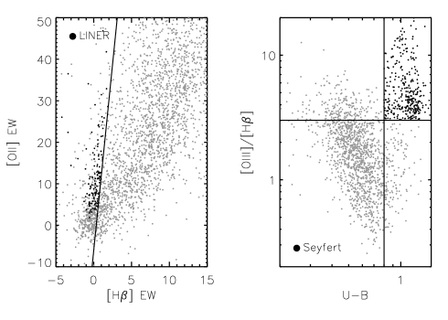
Figure 1: Two panels that show our AGN selection of Seyferts and LINERS within the DEEP2. The left panel plots [OII] EW versus ${\rm H{\beta}}$ EW for objects with accurate redshifts ($Q\geq 3$), $\delta_{3}$ environment measures, and covered [OII], [OIII] and ${\rm H{\beta}}$ (grey points). LINERs (black points) are selected using the empirical demarcation of Equation 1 along with the colour cut defined by Equation 2. The right panel shows the line ratio ${\rm[OIII]/H{\beta}}$ plotted against $(U-B)$ rest-frame colour for the same DEEP2 sample (grey points). Seyferts (black points) are selected to have ${\rm[OIII]/H{\beta}\geq 3}$ and rest-frame colour $(U\!-\!B)>0.8$, as denoted by the horizontal and vertical lines. See Section 2.1 for further details.

2 Galaxy and AGN Selection

Our primary galaxy and AGN samples are drawn from the DEEP2 Galaxy Redshift Survey (Davis et al., 2003, 2005), a project designed to study galaxy evolution and the underlying large-scale structure out to redshifts of $z\sim 1.4$. The survey utilises the DEIMOS spectrograph (Faber et al., 2003) on the 10-m Keck II telescope and has so far targeted $\lower 2.15277pt\hbox{$\;\buildrel>\over{\sim}\;$}50\,000$ galaxies covering $\sim 3$ square degrees of sky over four widely separated fields. In each field, targeted galaxies are observed down to an apparent magnitude limit of $R_{\rm AB}<24.1$. Important for this work, the spectral resolution of the DEIMOS spectrograph is quite high, ${\rm R}\approx 5000$, spanning an observed wavelength range of $6500\!<\!\lambda\!<\!9200$Å. This allows us to confidently identify AGN candidates through emission-line ratios down to low equivalent widths; such objects form a core part of the data analysed in this paper. More details on the DEEP2 survey design and galaxy detection can be found in Davis et al. (2003, 2005, 2007) and Coil et al. (2007).

To study the dependence of the AGN fraction on local environment, for each galaxy we use the pre-calculated projected third-nearest-neighbour distance, $D_{p,3}$, and surface density, $\Sigma_{3}=3/(\pi D_{p,3}^{2})$ (taken from Cooper et al., 2005). This density measure is then normalised by dividing by the mean projected surface density at the redshift of the galaxy in question, yielding a quantity denoted by $1+\delta_{3}$ . Tests using mock galaxy catalogues show that $\delta_{3}$ is a robust environment measure that minimises the role of redshift-space distortions and edge effects. See Cooper et al. (2005) for further details and comparisons with other commonly used density estimators.

To complement our optical catalogue we employ Chandra X-ray data from the All-Wavelength Extended Groth Strip International Survey (AEGIS, Davis et al. 2007). The AEGIS catalogue provides a panchromatic measure of the properties of galaxies in the Extended Groth Strip (EGS) covering X-ray to radio wavelengths. The EGS is part of DEEP2, constituting approximately one sixth of its total area. This allows us to cross-correlate each X-ray detection with the optical catalogue to identify each galaxy counterpart. In this way environments can be determined for the X-ray AGN sources.

Selecting objects from both the DEEP2 spectroscopic and Chandra (AEGIS) X-ray catalogues provides two different AGN populations that are embedded in the same underlying large-scale structure. To differentiate the two in the remainder of the paper, we hereafter refer to the first as the optically selected sample (OSS) and the second as the X-ray selected sample (XSS). In the following sections we describe the OSS and XSS populations in more detail.

2.1 The optically selected AGN sample (OSS)

Optically (or spectroscopically) selected AGN in the DEEP2 survey can be divided into two main classes, LINERs and Seyferts, distinguished primarily through the spectral lines present and their strength. Although the physical processes that differentiate one class from the other are still not well understood, the identification of each class is never-the-less well defined. We restrict our analysis to the redshift range $0.72\!<\!z\!<\!0.85$ to ensure that all chosen AGN spectral indicators are visible within the covered wavelength range and that the environment measure is sufficiently reliable. This will be the redshift interval from which all our OSS results are taken. Furthermore, to facilitate a fair comparison between both AGN types, only objects on the red sequence or in the green valley are included (defined below). This will also allow us to compare with a low redshift sample (see Section 4). For a complete discussion of the spectroscopic detection of AGN in the DEEP2 survey see Yan et al. 2007 (in prep.). Below we will briefly outline our LINER and Seyfert selection in turn.

2.1.1 LINERs

As discussed in Yan et al. (2006), LINERs are a population of emission-line galaxies with high equivalent width (EW) ratio ${\rm[OII]/H{\alpha}}$ (or ${\rm[OII]/H{\beta}}$). Specifically, we select a complete sample of LINERs using the division in ${\rm[OII]/H{\beta}}$ EW space given in Yan et al. (2006):

$${\rm EW\big{(}\big{[}O_{II}\big{]}\big{)}>18\,EW\big{(}H{\beta}\big{)}-6}$$ (1)

The left panel of Figure 1 illustrates this selection by plotting [OII] EW against ${\rm H{\beta}}$ EW for the entire DEEP2 sample with accurate redshifts ($Q\geq 3$), $\delta_{3}$ environment measures, covered [OII], [OIII] and ${\rm H{\beta}}$ (for consistency with Seyfert selection – see below), and redshift window $0.72\!<\!z\!<\!0.85$ (grey points). The solid line indicates the empirical demarcation of Equation 1. Since quiescent galaxies with no line emission also satisfy this criteria, the inequality relation alone is not sufficient. Thus, we further require LINERs to have significant detection ($2\sigma$) of [OII]. As ${\rm H{\beta}}$ emission is expected to be weak in LINERs (Yan et al., 2006), we do not require significant detection on ${\rm H{\beta}}$.

The error on ${\rm H{\beta}}$ EW emission is large due to the difficulty in measuring it after subtracting the stellar absorption. The above LINER selection has contamination from star-forming galaxies whose ${\rm H{\beta}}$ EW is underestimated. From a study of SDSS galaxies, Yan et al. (2006) concluded that LINERs are almost exclusively found in red sequence galaxies. Therefore, we adopt an additional colour cut to remove this contamination, which is the same used by Willmer et al. (2006):

$${(U\!-\!B)>-0.032M_{B}+0.322}$$ (2)

Our final LINER sub-sample with all of the above constraints is comprised of 116 objects and is over-plotted in the left panel of Figure 1 with black points. Note that within the SDSS a strong vertical branch can be seen (see Figure 2 of Yan et al. 2006, where they use $\rm H{\alpha}$ instead of ${\rm H{\beta}}$). This branch is significantly weaker at $z\sim 1$ in the DEEP2 data. This is due in part to the greater errors on ${\rm H{\beta}}$ in the DEEP2 data, and in part to the domination of red galaxies in the SDSS sample (due to the SDSS selection criteria).

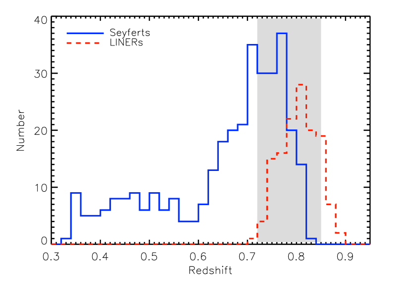
Figure 2: The redshift distribution for our optically selected AGN sample (OSS, Section 2.1). The distribution of Seyferts is given by the blue solid line, while the distribution of LINERs is given by the red dashed line. The shaded region denotes the redshift window $0.72\!<\!z\!<\!0.85$ from which our final OSS sample is drawn. Within this window both populations are cleanly identified spectroscopically and the effect of selection is small in both sub-samples.

2.1.2 Seyferts

Seyferts require different selection techniques than LINERs. Following the method of Yan et al (in prep.), we identify Seyferts in DEEP2 using a modified Baldwin-Phillips-Terlevich (BPT) diagram (Baldwin et al., 1981). Historically, the BPT diagram has been a reliable tool for determining the source of line emission from a galaxy. By plotting the line ratios ${\rm[OIII]\ \lambda 5007/H{\beta}}$ against ${\rm[NII]\ \lambda 6583/H{\alpha}}$ one can visually differentiate Seyferts, LINERs and star-forming galaxies. However, ${\rm H{\alpha}}$ is not available in the DEEP2 spectra at $z\lower 2.15277pt\hbox{$\;\buildrel>\over{\sim}\;$}0.4$ as it is redshifted into the infrared. For this reason, we use a modified BPT diagram which replaces the line ratio ${\rm[NII]\ \lambda 6583/H{\alpha}}$ with the rest-frame $U\!-\!B$ colour. This is possible because both are rough proxies for metallicity. Tests done on SDSS samples demonstrate that such a substitution is able to produce a clean and complete selection criterion for Seyferts (Yan et al. in prep.).

In the right panel of Figure 1 we illustrate our Seyfert selection by showing the modified BPT diagram for the same underlying sample used to select LINERs (grey points). This figure shows that the modified BPT diagram has a similar two branching structure to the original BPT diagram. Seyferts are selected to have ${\rm[OIII]/H{\beta}\geq 3}$ and rest-frame colour $(U\!-\!B)>0.8$ (horizontal and vertical lines, respectively). For cases in which ${\rm H{\beta}}$ is not positively detected, we use a $2\sigma$ lower limit on ${\rm[OIII]/H{\beta}}$. With such criteria we obtain 131 Seyferts in the range $0.72\!<\!z\!<\!0.85$ where all spectral signatures for both Seyferts and LINERs are normally available (black points). Selecting only red sequence (or green valley) objects facilitates a fair comparison with LINERs and is consistent with their typical position in the colour-magnitude diagram (Yan et al., 2006).

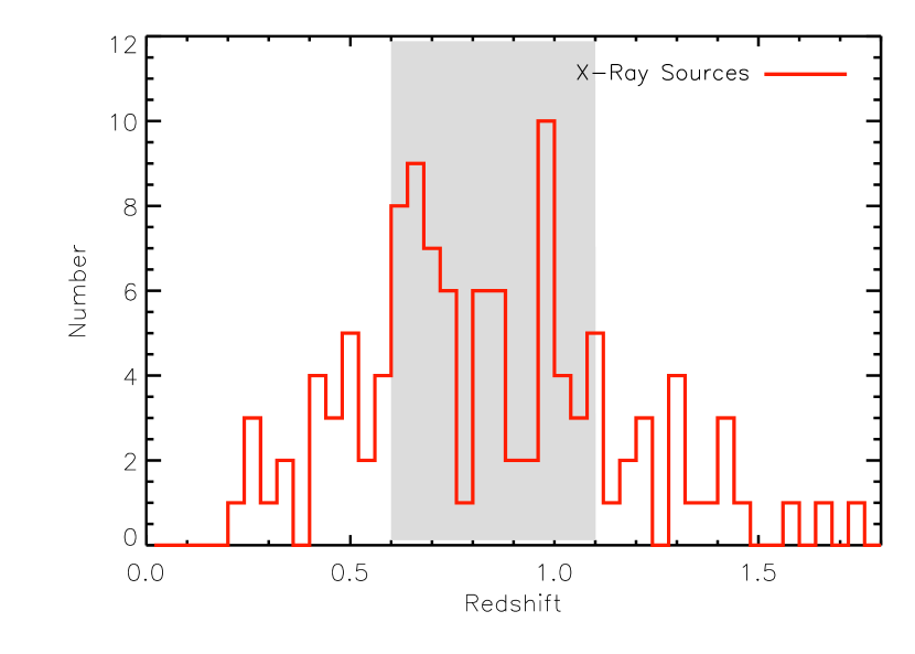
Figure 3: The redshift distribution for our X-ray selected AGN sample (XSS, Section 2.2), shown by the red solid line. The grey shaded region denotes the redshift range $0.6\!<\!z\!<\!1.1$, from which our final XSS is drawn. This range was chosen to be approximately comparable to the OSS (Figure 2) while simultaneously maximising the number and completeness in the sample.

2.1.3 Redshift distributions

In Figure 2 we show the redshift distribution of both LINERs (dashed line) and Seyferts (dotted line) drawn from the selection given in each panel of Figure 1. The DEEP2 Seyfert population extends from $z\approx 0.35$ to $z\approx 0.85$, peaking at around $0.75$. For LINERs the distribution is much more concentrated, extending from $0.72$ to $0.9$ and peaking at around $0.8$. Note that the peak for both is dominated by the DEEP2 survey galaxy selection and not an intrinsic peak in the AGN distribution. As discussed previously, the redshift window where both populations can be cleanly identified spectroscopically is $0.72\!<\!z\!<\!0.85$, denoted by the shaded region. This range maximises AGN coverage while insuring that selection effects are minimised in both samples.

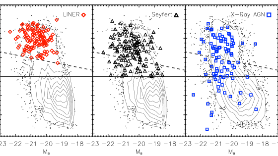
Figure 4: The colour-magnitude diagram (CMD) for LINERs (left panel, red diamonds), Seyferts (middle panel, black triangles) and X-ray AGN (right panel, blue squares). The demarcations given by the solid and dashed lines represent the conventions adopted to separate the blue cloud from the green valley, and the latter from red sequence objects (Equation 2), respectively (Willmer et al., 2006). The LINER sub-sample is composed of 116 objects, all of them lying on the red sequence by definition. The Seyferts sub-sample is composed of 131 objects, with 97 of them on the red sequence and 34 in the green valley. Finally, from our X-ray sample of 68 objects, 36 sources are red, 16 are green, and the remaining 16 blue. The underlying CMD of the population from which all AGN are drawn is shown in each panel with grey contours and black points. This parent population, in the left-hand and middle panels, is comprised of objects with accurate redshifts ($Q\geq 3$), $\delta_{3}$ environment measures, covered [OII], [OIII] and ${H{\beta}}$ ; and redshift between $0.72$ and $0.85$. In the right-hand panel, the grey contours and black points represent all objects in the EGS field with accurate redshifts ($Q\geq 3$) and $\delta_{3}$ environment measures; and redshift between $0.6$ and $1.1$.

2.2 The X-Ray selected AGN sample (XSS)

AEGIS Chandra X-ray sources within the EGS field are optically and spectroscopically identified by cross-correlating with the DEEP2 photometric and redshift catalogues, following the prescriptions presented by Georgakakis et al. (2007). They cover X-ray luminosities of $10^{41}\!\lower 2.15277pt\hbox{$\;\buildrel<\over{\sim}\;$}\!{\rm L_{X}(erg/s)}\!\lower 2.15277pt\hbox{$\;\buildrel<\over{\sim}\;$}\!10^{44}$ in host galaxies of luminosity $-19\!\lower 2.15277pt\hbox{$\;\buildrel<\over{\sim}\;$}\!M_{B}-5\log h\!\lower 2.15277pt\hbox{$\;\buildrel<\over{\sim}\;$}\!-22$. The base X-ray sample comprises a total of $113$ reliably matched objects.

In Figure 3 we show the redshift histogram of our X-ray catalogue. To extract a sample that is as closely comparable to the OSS as possible while simultaneously maximising AGN number and completeness, we restrict the X-ray sources to the redshift range $0.6\!<\!z\!<\!1.1$. This is wider than the OSS redshift window; however, both samples (OSS and XSS) have similar redshift means, and we assume that the evolution effects for sources outside the OSS redshift window do not dominate our results (or at least does not differ significantly from evolution in the red sequence population itself). In this redshift range the number of reliable X-ray AGN drops to $68$, including $52$ red-ward of $(U\!-\!B)>0.8$ (i.e. a green valley cut), and $36$ red-ward of Equation 2 (i.e. a red sequence cut).

2.3 AGN in colour-magnitude space

In Figure 4 we show the colour-magnitude diagram (CMD) for LINERs (left panel), Seyferts (middle panel) and X-ray AGN (right panel). The demarcations given by the solid and dashed lines represent the conventions adopted to separate the blue cloud from the green valley, and the latter from red sequence objects (Equation 2), respectively (Willmer et al. 2006; Yan et al. in prep.). Here, LINERs are red sequence galaxies by definition. As explain above, this restriction is supported by the fact that local LINERs are almost exclusively red (Yan et al., 2006). For Seyferts, $\sim 80\%$ lie on the red side of the CMD, with the remainder residing in the green valley. Finally, for the XSS AGN, $\sim 50\%$ of the sources are red, $\sim 25\%$ are green, and the remaining $\sim 25\%$ blue. The grey contours in each panel show the underlying DEEP2 CMD within the same redshift range.

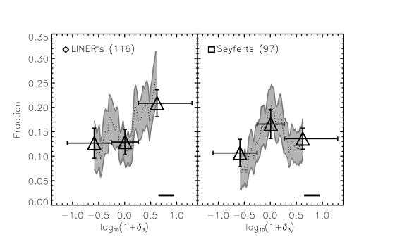
Figure 5: The AGN fraction in red sequence galaxies versus local galaxy over-density, $\delta_{3}$, for LINERs (left panel) and Seyferts (right panel). For each, the respective symbols (diamonds for LINERs and squares for Seyferts) show the median measure in bins of low, mean and high density. Vertical error-bars represent the Poissonian uncertainty, while horizontal error-bars show the size of each density range. We also show how the AGN fraction varies smoothly with environment using a sliding box of width $0.3$ dex shifted from low to high density in increments of $0.025$ dex (dotted lines with shaded area showing the $1\sigma$ uncertainty in the sliding fraction). The overall fraction of LINERs and Seyferts is plotted with horizontal dashed lines. This figure shows some evidence that LINERs tend to favour high density environments relative to the underlying red sequence, whereas Seyferts have little (or no) environment dependencies.

2.4 Errors and completeness

Our greatest source of error is that of noise from small number statistics, given the low number of AGN we have available in the DEEP2 and AEGIS surveys in any particular environment bin. Such current generation high redshift catalogues are thus still limited in the extent to which the statistical nature of the AGN population can be examined. All errors calculated in this paper were determined by propagating the Poissonian uncertainties on the number of objects. Due to the small number statistics, the errors obtained with this method will dominate any cosmic variance effects in the observed fields (Newman & Davis, 2002).

It should be noted that the DEEP2 survey is by design incomplete. At $z\sim 1$, approximately $60\%$ of the actual objects are observed by the telescope. Moreover, redshifts are successfully obtained for around $70\%$ of the target parent population (based on tests with blue spectroscopy, most failures are objects at z¿1.4 (Steidel, priv. comm.)). This should be carefully considered in any statistic that counts absolute numbers of objects. In our work, however, we deal with relative numbers of objects, i.e. the AGN fraction. We assume, to first order (and to the level of uncertainty given by the Poisson error), that any variation in redshift success or targeting rate between the AGN sample and the red sequence parent population is the same in low density regions as it is in high density regions. In principle, one may expect an easier detection (or even an easier redshift estimation) of an object identified as an AGN than the one for a “regular” red sequence object (due to the presence of remarkable features in the spectrum). However both Cooper et al. (2005) and Gerke et al. (2005) found that DEEP2 selection rates are essentially independent of local density.

Finally, because of the different Seyfert and LINER selection we find some inevitable (but small) overlap between the two populations, $7\%$ of the total in our case, where a single object has been classified as both AGN types. We have re-calculated all our results excluding these dual class objects and find only trivial differences. For the sake of maximising statistics we have not removed such objects from the OSS, however note that they may constitute an interesting sub-population whose physical implications warrant further investigation.

3 Results

In this section we present our primary result: the dependence of the AGN fraction in the red sequence on local environment density. We will also extend the analysis to include green valley objects.

Figure 5 presents the density dependence of the fraction of $z\sim 1$ red sequence AGN, for LINERs (left panel) and Seyferts (right panel) separately. In each panel, the respective symbols show the median measure in bins of low, mean and high density environments (each of them encompassing one third of the OSS), where the horizontal error-bars indicate the width of each bin, and the vertical error-bars show the Poisson uncertainty in the measured fraction, as described in Section 2.4. We also show how the AGN fraction varies smoothly with environment using a sliding box of width $0.3$ dex, shifted from low to high density in intervals of $0.025$ dex (dotted line). The accompanying grey-shaded regions correspond to the sliding $1\sigma$ uncertainties in the sliding fraction.

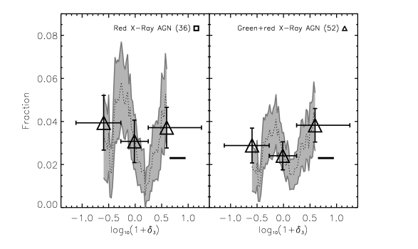
Figure 6: The AGN fraction versus environment for our X-ray selected sample (XSS), using the same format as in Figure 5. In the left panel, squares show the fraction of red sequence X-ray AGN in the three density bins considered. In the right panel we extend this analysis to include green valley AGN. Note that this extension does not change the results in any significant way. XSS AGN behave more like Seyferts than LINERs (see Figure 5), with the fraction showing only a weak (or no) environmental dependence to within the errors.

Evidence for a trend in the behaviour of the LINERs is quite apparent in Figure 5, suggesting the possibility that these objects tend to favour high density environments, and in a way stronger than the majority of red sequence galaxies. This is in contrast to the behaviour of red Seyferts, which show little (or no) environment dependence relative to the red sequence. This is a key result that will be discussed in more detail in the following sections.

We now consider the X-ray catalogue drawn from the AEGIS Chandra imaging. Figure 6 presents the X-ray selected AGN fraction versus local environment (note that the same format used in Figure 5 has been applied here). In the left panel we show the fraction of red X-Ray AGN and in the right panel we extended the analysis to include green valley X-ray AGN and galaxies. Including green valley objects does not significantly alter our results. Red sequence X-ray selected AGN appear to behave similarly to optically selected Seyferts in terms of their lack of environmental preference, and differently from the LINER population in high density environments. This is in agreement with the results of Georgakakis et al. (2007), also using the AEGIS data. We note that improved statistics could show trends at levels equal to or smaller than that which can be measured here given our errors.

We have tested the significance of the results in Figures 5 and 6 in a number of ways. Since LINERs show the most interesting environment dependencies we will focus our tests on this population. We randomly draw $1000$ sub-samples from the red sequence and replace the LINER sample with each of these random populations. After repeating our analysis for each we find that only $2\%$ of the random sub-samples show similar density dependencies to the LINER population (i.e. results at least as pronounced as the one in Figure 5) . The LINER environment dependence seen in the left panel of Figure 5 deviates by at least $2\sigma$ (actually almost $2.5\sigma$) from a random selection of red sequence galaxies. Additionally, we can confirm that the trend in Figure 5 is not due to an implicit dependence of colour or magnitude on environment within the red sequence. This was checked by repeatedly replacing the LINER sample with randomly drawn objects with the same colour or colour and magnitude distributions, and comparing their density distributions with that of the real LINERs. The mean density of the LINER population is $1+\delta_{3}=0.37\pm 0.06$, almost double that for randomly colour selected samples which have $1+\delta_{3}=0.20\pm 0.01$, and randomly colour and magnitude selected samples with $1+\delta_{3}=0.19\pm 0.01$. Similar tests were performed on Seyferts and X-Ray AGN.

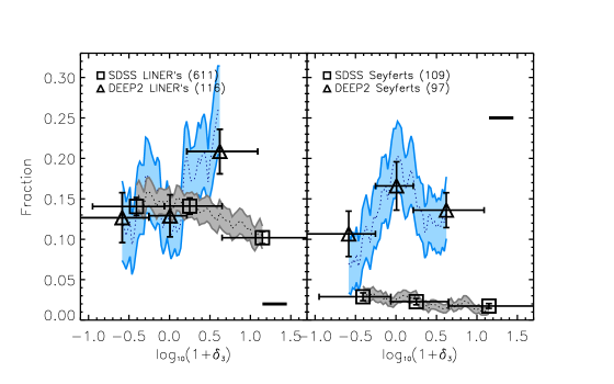
Figure 7: The SDSS red sequence AGN fractions versus environment, plotted using the same format from Figures 5 and 6. The left panel shows the fraction of low-z SDSS LINERs (squares) and, for comparison, the high-z DEEP2 LINER fraction (triangles) reproduced from Figure 5. The right panel shows the fraction of SDSS Seyferts, with the equivalent DEEP2 result again reproduced from Figure 5 for comparison. SDSS LINERs and Seyferts both show a decreasing AGN fraction towards high density environments, unlike that seen in DEEP2. At $z\sim 1$, LINERs and Seyferts are approximately equally abundant, whereas by $z\sim 0$ the relative abundance of Seyferts to LINERs has dropped by approximately a factor of $7$.

4 A Comparison with Local AGN in the SDSS

Our results thus far suggest that the $z\sim 1$ red sequence LINER fraction depends on environment in a way that is different from Seyferts. This dependence takes the form of an increase in the relative abundance of LINERs in higher density environments. In this section we address the question of AGN fraction evolution. Specifically, do local red sequence LINERs also favour dense environments and Seyferts show little environment dependence?

Our low redshift AGN sample is drawn from the Sloan Digital Sky Survey (SDSS, York et al. 2000) spectroscopic DR4 catalogue (Adelman-McCarthy et al., 2006). The SDSS DR4 covers almost $5000$ square degrees of the sky in five filters ($ugriz$) to an apparent magnitude limit of $r=17.7$. The redshift depth is approximately $z\sim 0.3$, with a median redshift of $z=0.1$. DR4 consists of $\sim 400\,000$ galaxies. The same environment measure is applied for consistency with the DEEP2 analysis above (see Cooper et al. 2007a for full details).

To measure the low redshift AGN fraction we follow a similar procedure to that used for the high-z results. This procedure isolates a well defined red sequence population and identifies AGN within it. The base red sequence population is constructed by selecting SDSS galaxies within the redshift interval $0.05\!<\!z\!<\!0.15$ and applying the rest-frame colour cut $(U-B)>-0.032M_{B}+0.483$ (Cooper et al. 2007a, in agreement with the previous analysis by Blanton 2006). For consistency with our DEEP2 sample we take a faint absolute magnitude limit of $M_{\rm B}-5\log h=-20$ (representing the approximate faint-end of the red sequence at $z\sim 0.8$ within the DEEP2 data) and evolve it $0.88$ magnitudes to mimic the evolution in the galaxy luminosity function between DEEP2 and SDSS (assuming evolution of $1.3$ magnitudes per unit redshift from Willmer et al. 2005 and mean DEEP2 and SDSS redshifts of $0.78$ and $0.1$, respectively). With these constraints the underlying low-z red galaxy sample is composed of $5335$ objects.

To select AGN from the SDSS red sequence sample we use the same set of criteria described in Section 2.1 with the following modifications. Since SDSS spectra have a much higher signal-to-noise than DEEP2 spectra the emission line detections are easier. This will result in differences between the two AGN samples, as SDSS AGN will include weaker optical AGN than the DEEP2 can detect. Therefore, we determine a different line detection criterion by comparing the errors in the emission line EW measurements. Typical line measurement errors in DEEP2 are almost exactly twice as large as those in SDSS. We thus change all $2\sigma$ line detection criteria to $4\sigma$ for selecting AGN in the SDSS. The final low redshift AGN sample is comprised of $720$ objects, $611$ being LINERs and $109$ Seyferts. This should be contrasted with the high-z sample which has $213$ objects, of which $116$ are LINERs and $97$ Seyferts.

In Figure 7 we present the SDSS red sequence AGN fractions versus environment (this figure follows the same format used in Figures 5 and 6). The left panel shows the fraction of local red sequence LINERs (squares) and, for comparison, the high redshift LINER fraction (triangles) reproduced from Figure 5. The right panel shows the Seyfert fraction in the SDSS red population (squares) and similarly for DEEP2 (triangles, from Figure 5).

The left panel of Figure 7 reveals a different LINER trend with environment at $z\sim 0$ than that seen at $z\sim 1$. LINERs in the SDSS show no indication of favouring high density regions relative to other environments. In fact, it is very statistically significant that SDSS LINERs tend to reside more in mean-to-low density environments and clearly disfavour those of high density. In the right panel of Figure 7 Seyferts also follow a clear trend of decreasing AGN fraction towards denser SDSS environments. This is in contrast to the weak (or no) environmental trend in the high redshift DEEP2 Seyfert population.

It is important to note that comparing the overall amplitudes of the LINER and Seyfert fractions between DEEP2 and SDSS is dangerous, as subtleties in the selection of the underlying red sequence can shift the absolute values around somewhat. The relative trends across environment within a population are much more robust however, and these can be compared between high and low redshift (for example, we do not expect any selection effects to have a significant density dependence). Additionally, the difference in the abundance between Seyferts and LINERs at a given redshift can be contrasted. Seyferts and LINERs are approximately equally abundant at $z\sim 1$. By $z\sim 0$ however, the Seyfert population has diminished relative to the LINER population by over a factor of $7$. This decline in the relative number of Seyfert AGN by redshift zero will be discussed in the next section.

5 Discussion

5.1 Previous measures of AGN and environment

It is difficult to make direct comparisons of our results with previously published works. This is because past environment studies have tended to focus on the AGN fraction of all colours of host galaxies, and also to mix both LINER and Seyfert classes into a combined AGN population. Our selection is restricted to the red sequence only (and also green valley), which allows us to compare high and low redshift populations and also study the AGN–environment connection without the colour–environment correlation.

Locally, a number of SDSS measures of AGN and environment have been made. Using the SDSS early data release, Miller et al. (2003) found no dependence on environment for the spectroscopically selected AGN fraction in a sample of 4921 objects. Specifically, the authors report no statistically significant decrease in the AGN fraction in the densest regions, although their densest points visually suggest such a trend. This result is broadly consistent with the results of both LINERs and Seyferts in Figure 7, even though we only consider red sequence objects.

Kauffmann et al. (2003) also found little environment dependence of the overall fraction of detected AGN in a sample drawn from the SDSS DR1. However, they do report different behaviour when the sample is broken into strong AGN ($\log L[{\rm OIII}]>7$, “Seyferts”) and weak AGN ($\log L[{\rm OIII}]<7$, “LINERs”). For Seyfert they find a significant preference for low-density environments, especially when hosted by more massive galaxies. This is consistent with our SDSS findings in Figure 7 and different to what we find at $z\sim 1$ in the DEEP2 fields. For LINERs, Kauffmann et al. measure little environment dependence, whereas we find a significant decline in the SDSS LINER fraction in our overdense bins. The explanation for this difference may come from our removal of possible contaminating star forming galaxies by restricting our analysis to the red sequence. Also, we impose a higher line detection threshold on the SDSS data to provide a fair comparison with DEEP2 (see Section 4). Finally, Kauffmann et al. (2003) required that all lines for the BPT diagnosis were detected and this implies biasing the LINERs sample towards the strongest objects.

Between redshifts $z=0.4$ and $z=1.35$, Cooper et al. (2007a) show that red galaxies within the DEEP2 survey favour overdense environments, although the blue fraction in clusters does become larger as one moves to higher redshift (see also Gerke et al., 2007; Coil et al., 2007). At all redshifts there exists a non-negligible red fraction in underdense environments, which evolves only weakly if at all. Nandra et al. (2007) show that the host DEEP2 galaxies of X-ray selected AGN within the EGS field ($\sim 1/6$ of the DEEP2 survey volume) occupy a unique region of colour-magnitude space. These objects typically live at the top of the blue cloud, within the green valley, or on the red sequence. Georgakakis et al. (2007) measure the mean environment of this population and confirm that, on average, they live in density regions above that of the mean of the survey. They find this to be true for all host galaxy magnitudes studied ($M_{B}\lower 2.15277pt\hbox{$\;\buildrel<\over{\sim}\;$}-21$) and colours ($U-B\lower 2.15277pt\hbox{$\;\buildrel>\over{\sim}\;$}0.8$) (note the DEEP2 red sequence begins at $U-B\sim 1$). However, given limited sample sizes, they were not able to establish whether the environment distribution of the X-ray AGN differed from that of the red population, rather than the DEEP2 population as a whole.

5.2 Understanding the sequence of events

From our results alone a comprehensive understanding of the different environment trends within the AGN population from high to low redshift is not possible. However, some speculation and interpretation can be made by drawing on our broader knowledge of these active objects from the literature.

One possible scenario posits that LINERs and Seyferts occur in different types of galaxies. In this picture, LINERs are often associated with young red sequence galaxies (Graves et al., 2007) and are especially common among post-starburst (K+A) galaxies (Yan et al., 2006). These galaxies would already be into the quenched phase of their evolution but still relatively young. Merger triggered starbursts and subsequent quasar winds are a possible mechanisms to produce rapid star formation shut down in such objects (Hopkins et al., 2006). The gas rich merging events required in this scenario are common in overdense environments at $z\sim 1$ as clusters and massive groups assemble. By $z\sim 0$, however, the activity in these environments has mostly ended. Hence, if this picture is correct, one may expect an over-abundance of red sequence LINERs in dense environments at high redshift (since both star formation and rapid quenching is common) that is not seen locally. This may be consistent with the trends found in the left panel of Figure 7.

Seyfert galaxies, on the other hand, could be objects in transition from the blue cloud to red sequence (Groves et al., 2006), whose AGN are thought to be initiated by internal processes (and not mergers), inferred from their often found spiral structure (e.g. M77) (mergers act to destroy such structure). From this, one may expect our red sequence Seyfert population to represent the tail of the colour distribution of transitioning objects whose dependence on environment is determined by secular mechanisms and who would evolve accordingly. At high redshift, disk galaxies are commonly found in all environments, including the most dense. In contrast, overdense regions in the local Universe are dominated by passive ellipticals and show an absence of spirals. This would be broadly consistent with our findings in the right panel of Figure 7, where the most significant evolution in the red Seyfert fraction arises from a depletion in overdense regions relative to other environments, from high redshift to low.

Alternatively, some authors claim that LINERs and Seyferts form a continuous sequence, with the Eddington rate the primary distinguishing factor (Kewley et al., 2006). In this scenario, Seyferts are young objects with actively accreting black holes. As the star formation begins to decay so does the accretion rate, and the galaxy enters a transition phase. Eventually, a LINER-like object emerges, with an old stellar population and very low supermassive BH accretion rate. This picture is supported by recent studies in voids from Constantin et al. (2007). At high redshift, our results show that red Seyferts and LINERs are approximately equally abundant. By $z\sim 0$ however, the Seyfert population has declined relative to the LINER population by over a factor of $7$. This may be interpreted as the natural transformation of Seyferts into LINERs with time, within a galaxy population which is smoothly reddening from $z\sim 1$ to $z\sim 0$. Moreover, the fact that high-z LINERs reside preferentially in high-density environments may imply that this Seyfert-LINER transition is more efficient in dense regions of the Universe.

6 Summary

In this paper we measure the dependence of the AGN fraction of red galaxies on environment in the $z\sim 1$ DEEP2 Galaxy Redshift Survey and local $z\sim 0.1$ SDSS. We restrict our analysis to the red sequence to maintain a clean and consistent selection of AGN at high and low redshift, and this also reduces the additional effects of environment associated with galaxy colour.

Our results can be summarised as follows:

• High redshift LINERs at $z\sim 1$ in DEEP2 appear to favour higher density environments relative to the red sequence from which they are drawn. In contrast, Seyferts and X-ray selected AGN at $z\sim 1$ show much weaker (or no) environmental dependencies within the same underlying population. Extending our analysis to include green valley objects has little effect on the results.

• Low redshift LINER and Seyfert AGN in the SDSS both show a slowly declining red sequence AGN fraction towards high density environments. This is in contrast to the high redshift result.

• At $z\sim 1$, Seyferts and LINERs are approximately equally abundant. By $z\sim 0$ however, the Seyfert population has declined relative to the LINER population by over a factor of $7$.

It is important to remember that such measures are difficult to make with current data, and hence we remain limited by statistics to the extent to which we can physically interpret our results. Regardless, a robust outcome of our analysis is the differences between LINER and Seyfert AGN populations in high density regions, and between high and low redshift in all environments. Our results indicate that a greater understanding of both AGN and galaxy evolution may be possible if future analyses simultaneously focus on the detailed subdivision of different AGN classes, host galaxy properties, and their environment.

References

- Adelman-McCarthy et al. (2006) Adelman-McCarthy J. K., Agüeros M. A., Allam S. S., et al., 2006, ApJS, 162, 38
- Baldwin et al. (1981) Baldwin J. A., Phillips M. M., Terlevich R., 1981, PASP, 93, 5
- Balogh et al. (2004) Balogh M. L., Baldry I. K., Nichol R., Miller C., Bower R., Glazebrook K., 2004, ApJL, 615, L101
- Best (2004) Best P. N., 2004, MNRAS, 351, 70
- Blanton (2006) Blanton M. R., 2006, ApJ, 648, 268
- Blanton et al. (2005) Blanton M. R., Eisenstein D., Hogg D. W., Schlegel D. J., Brinkmann J., 2005, ApJ, 629, 143
- Bower et al. (2006) Bower R. G., Benson A. J., Malbon R., et al., 2006, MNRAS, 370, 645
- Bundy et al. (2006) Bundy K., Ellis R. S., Conselice C. J., et al., 2006, ApJ, 651, 120
- Coil et al. (2007) Coil A. L., Newman J. A., Croton D., et al., 2007, ArXiv e-prints, 708
- Constantin et al. (2007) Constantin A., Hoyle F., Vogeley M. S., 2007, ArXiv e-prints, 710
- Constantin & Vogeley (2006) Constantin A., Vogeley M. S., 2006, ArXiv Astrophysics e-prints
- Cooper et al. (2007a) Cooper M. C., Newman J. A., Coil A. L., et al., 2007a, MNRAS, 376, 1445
- Cooper et al. (2006) Cooper M. C., Newman J. A., Croton D. J., et al., 2006, MNRAS, 370, 198
- Cooper et al. (2005) Cooper M. C., Newman J. A., Madgwick D. S., Gerke B. F., Yan R., Davis M., 2005, ApJ, 634, 833
- Cooper et al. (2007b) Cooper M. C., Newman J. A., Weiner B. J., et al., 2007b, ArXiv e-prints, 706
- Croton et al. (2006) Croton D. J., Springel V., White S. D. M., et al., 2006, MNRAS, 365, 11
- Cucciati et al. (2006) Cucciati O., Iovino A., Marinoni C., et al., 2006, A&A, 458, 39
- Davis et al. (2005) Davis M., DEEP Team, Extended Groth Strip Collaboration, 2005, in Bulletin of the American Astronomical Society, vol. 37 of Bulletin of the American Astronomical Society, 1299–+
- Davis et al. (2003) Davis M., Faber S. M., Newman J., et al., 2003, in Discoveries and Research Prospects from 6- to 10-Meter-Class Telescopes II. Edited by Guhathakurta, Puragra. Proceedings of the SPIE, Volume 4834, pp. 161-172 (2003)., edited by P. Guhathakurta, vol. 4834 of Presented at the Society of Photo-Optical Instrumentation Engineers (SPIE) Conference, 161–172
- Davis et al. (2007) Davis M., Guhathakurta P., Konidaris N. P., et al., 2007, ApJL, 660, L1
- Dressler (1980) Dressler A., 1980, ApJ, 236, 351
- Dressler & Gunn (1983) Dressler A., Gunn J. E., 1983, ApJ, 270, 7
- Elbaz et al. (2007) Elbaz D., Daddi E., Le Borgne D., et al., 2007, A&A, 468, 33
- Faber et al. (2003) Faber S. M., Phillips A. C., Kibrick R. I., et al., 2003, in Instrument Design and Performance for Optical/Infrared Ground-based Telescopes. Edited by Iye, Masanori; Moorwood, Alan F. M. Proceedings of the SPIE, Volume 4841, pp. 1657-1669 (2003)., edited by M. Iye, A. F. M. Moorwood, vol. 4841 of Presented at the Society of Photo-Optical Instrumentation Engineers (SPIE) Conference, 1657–1669
- Georgakakis et al. (2007) Georgakakis A., Nandra K., Laird E. S., et al., 2007, ApJL, 660, L15
- Gerke et al. (2005) Gerke B. F., Newman J. A., Davis M., et al., 2005, ApJ, 625, 6
- Gerke et al. (2007) Gerke B. F., Newman J. A., Faber S. M., et al., 2007, MNRAS, 376, 1425
- Graves et al. (2007) Graves G. J., Faber S. M., Schiavon R. P., Yan R., 2007, ArXiv e-prints, 707
- Groves et al. (2006) Groves B., Kewley L., Kauffmann G., Heckman T., 2006, New Astronomy Review, 50, 743
- Hogg et al. (2004) Hogg D. W., Blanton M. R., Brinchmann J., et al., 2004, ApJL, 601, L29
- Hogg et al. (2006) Hogg D. W., Masjedi M., Berlind A. A., Blanton M. R., Quintero A. D., Brinkmann J., 2006, ApJ, 650, 763
- Hopkins et al. (2006) Hopkins P. F., Somerville R. S., Hernquist L., Cox T. J., Robertson B., Li Y., 2006, ApJ, 652, 864
- Kauffmann et al. (2003) Kauffmann G., Heckman T. M., Tremonti C., et al., 2003, MNRAS, 346, 1055
- Kauffmann et al. (2004) Kauffmann G., White S. D. M., Heckman T. M., et al., 2004, MNRAS, 353, 713
- Kewley et al. (2006) Kewley L. J., Groves B., Kauffmann G., Heckman T., 2006, MNRAS, 372, 961
- Le Fevre et al. (2003) Le Fevre O., Vettolani G., Maccagni D., et al., 2003, in Discoveries and Research Prospects from 6- to 10-Meter-Class Telescopes II. Edited by Guhathakurta, Puragra. Proceedings of the SPIE, Volume 4834, pp. 173-182 (2003)., edited by P. Guhathakurta, vol. 4834 of Presented at the Society of Photo-Optical Instrumentation Engineers (SPIE) Conference, 173–182
- Miller et al. (2003) Miller C. J., Nichol R. C., Gómez P. L., Hopkins A. M., Bernardi M., 2003, ApJ, 597, 142
- Nandra et al. (2007) Nandra K., Georgakakis A., Willmer C. N. A., et al., 2007, ApJL, 660, L11
- Newman & Davis (2002) Newman J. A., Davis M., 2002, ApJ, 564, 567
- Nolan et al. (2007) Nolan L. A., Raychaudhury S., Kabán A., 2007, MNRAS, 375, 381
- Oemler (1974) Oemler A. J., 1974, ApJ, 194, 1
- Sorrentino et al. (2006) Sorrentino G., Radovich M., Rifatto A., 2006, A&A, 451, 809
- Wake et al. (2004) Wake D. A., Miller C. J., Di Matteo T., et al., 2004, ApJL, 610, L85
- Willmer et al. (2005) Willmer C. N. A., Faber S. M., Koo D. C., et al., 2005, ArXiv Astrophysics e-prints
- Willmer et al. (2006) Willmer C. N. A., Faber S. M., Koo D. C., et al., 2006, ApJ, 647, 853
- Yan et al. (2006) Yan R., Newman J. A., Faber S. M., Konidaris N., Koo D., Davis M., 2006, ApJ, 648, 281
- York et al. (2000) York D. G., Adelman J., Anderson Jr. J. E., et al., 2000, AJ, 120, 1579
- Zirbel (1997) Zirbel E. L., 1997, ApJ, 476, 489