Family symmetries
and the origin of fermion masses and mixings

Abstract

Family symmetries are possibly the most conservative extension of the Standard Model that attempt explanations of the pattern of fermion masses and mixings. The observed large mixing angles in the lepton sector may be the first signal for the presence of a non-Abelian family symmetry. We investigate the possibilities of simultaneously explaining the observed pattern of masses of the quarks (hierarchical masses and small mixing angles) and of the leptons (near tri-bi-maximal mixing, thus large mixing angles). We show that such contrasting observations can be achieved naturally via the seesaw mechanism, whether in models with continuous or discrete family symmetries.

We consider also in some detail the constraints on flavour changing neutral currents arising from introducing a continuous family symmetry. We show that, for a restricted choice of the flavon sector, continuous family symmetries are consistent with even the most conservative limits both for the case of gauge mediated supersymmetry breaking and the case of gravity mediated supersymmetry breaking.

This thesis is dedicated to my wife
Ana
for being herself

Chapter 1 Introduction

1.1 Motivation and outline

While the Standard Model extended to include right-handed neutrinos continues to successfully describe all existing data, there are sound theoretical reasons to believe that there is physics beyond the Standard Model. Appealing extensions of the Standard Model often include supersymmetry (SUSY), as well as Grand (GUTs) . Very brief reviews of both can be found in subsections 1.2.2 and 1.2.3.

The question why we have three generations of each type of fundamental fermion remains without a convincing answer. In the Standard Model the masses and mixings of all these fermions are simply parameters (the Yukawa couplings) that need to be measured. When going beyond the Standard Model, those fermion masses and mixings can arise through underlying mechanisms - examples of such being Froggatt-Nielsen, or the seesaw mechanism, two mechanisms that generate fermion masses through higher dimension operators involving heavier particles (both reviewed in section 1.4).

The data from neutrino oscillations (reviewed in subsection 1.2.4) compounds the puzzle of the fermion masses and mixings. The data indicates that the leptonic mixing angles are large - in stark contrast with the small mixing angles of the quark sector.

In the rest of chapter 1 we briefly review the current status of fermion masses and mixings, giving a very brief summary of the Standard Model, SUSY, GUTs and of neutrino oscillations. We then present a family symmetry review, briefly discussing recent models in the literature and illustrating the main points by using a very simple $U(1)_{f}$ toy model, motivating us to conclude the chapter with a review of the Froggatt-Nielsen mechanism and of the seesaw mechanism.

Chapter 2 presents original work on explaining the observed fermion masses and mixings data with continuous family symmetries, namely an $SU(3)_{f}$ family symmetry model. The vacuum expectation value alignment is then discussed (with more details in appendix A). The messenger sector involved in the respective Froggatt-Nielsen mechanism is also presented. The chapter concludes with the phenomenological implications of the model and a brief discussion regarding the cancellation of anomalies.

In chapter 3 we present original work on approaching the fermion masses and mixings problem with discrete family symmetries. We start by presenting a simple but incomplete model based on the group $\Delta(12)$. Then we continue by studying a model based on the group $\Delta(27)$. The novel vacuum expectation value alignment mechanism used in the $\Delta(27)$ model is discussed in detail and then the chapter is concluded with the phenomenological predictions of the model.

Chapter 4 contains original work on solving the family symmetry flavour problem (associated with continuous family symmetries). The topic is introduced by first re-examining the SUSY flavour problem and then identifying the contributions related to the continuous family symmetries. A simple $U(1)_{f}$ model serves to illustrate the problem. We conclude the chapter using the same model to also illustrate possible solutions that apply in the general case. The solutions are discussed in relation to the respective SUSY breaking mechanism (gravity or gauge mediated).

Finally, in chapter 5 we present a global conclusion and summary of the thesis.

1.2 Fermion masses and mixings

1.2.1 Standard Model

The Standard Model is a quantum field theory describing the fundamental particles and their interactions, based in the local gauge group $SU(3)_{C}\times SU(2)_{L}\times U(1)_{Y}$. The $SU(3)_{C}$ is the group of quantum chromodynamics (QCD), the theory of strong interactions of the coloured particles such as gluons (the gauge bosons of QCD) and quarks. The $SU(2)_{L}\times U(1)_{Y}$ is the group of the electroweak interaction, whose gauge bosons include the weak gauge bosons $W^{+}$, $W^{-}$ and $Z^{0}$, as well as the photon $\gamma$ of electromagnetic interactions; the electric charge is given by $Q_{em}=T_{3_{L}}+Y/2$ (the isospin $T_{3_{L}}$ is associated with $SU(2)_{L}$ and the hypercharge $Y$ is the $U(1)_{Y}$ quantum number).

The matter content of the Standard Model consists of three families of quarks and leptons. They transform as spinors under the Lorentz group, and as the left-handed and right-handed parts are treated differently under the gauge group, it is often more convenient to use 2 component Weyl spinors (dotted and undotted) rather than the Dirac spinor representation, although they are equivalent: the 4 component Dirac spinor $\Psi$ is composed of one undotted, or left-handed, 2 component spinor $\zeta_{\alpha}$ and one dotted, or right-handed, 2 component spinor $\eta^{\dagger\dot{\alpha}}$.

$$\Psi=\left(\begin{array}[]{c}\zeta_{\alpha}\\ \eta^{\dagger\dot{\alpha}}\end{array}\right)$$ (1.1)

If the 4 component Dirac spinor has the same dotted and undotted Weyl spinors ($\eta\equiv\zeta$), it is called a Majorana spinor (the left-handed and right-handed spinors are equivalent). The hermitian conjugate of a left-handed spinor is a right-handed spinor and vice-versa:

$$\left(\eta^{\dagger\dot{\alpha}}\right)^{\dagger}=\eta^{\alpha}$$ (1.2)

Finally, the case (upper or lower) of the indices is relevant, and they can be raised or lowered with the appropriate anti-symmetric Levi-Civita tensors $\epsilon^{\alpha\beta}$ or $\epsilon_{\alpha\beta}$ (or the dotted versions): $\zeta^{\alpha}\equiv\epsilon^{\alpha\beta}\zeta_{\beta}$ and so on. In general we will omit the spinor indices for simplicity, with the convention that two left-handed Weyl spinors contract as $\zeta\eta\equiv\zeta^{\alpha}\eta_{\alpha}$ and two right-handed spinors contract as $\zeta^{\dagger}\eta^{\dagger}=\zeta^{\dagger}_{\dot{\alpha}}\eta^{\dagger\dot{\alpha}}$.

We will use two distinct notations for the fermions, and it is useful to keep in mind that the charge conjugate $f^{c}$ of a right-handed fermion $f_{R}$ transforms in the same way as a left-handed fermion (see eq.(1.2)). We denote the true left-handed fermions either as $f$ or explicitly as $f_{L}$, so although similar it is important not to confuse $f^{c}$ with the charge conjugate of $f$, $f^{C}$. We won’t mix notations, so we either use $f$ together with $f^{c}$, or particularly in chapter 4, $f_{L}$ together with $f_{R}$ (usually we use only $f$ and $f^{c}$, as in that case we deal solely with fields that transform as left-handed fermions - very useful when discussing GUTs).

Each Standard Model family contains one left-handed quark doublet $Q=(u,d)$, one right-handed up type quark $u^{c}$, one right-handed down type quark $d^{c}$, one left-handed lepton doublet $L=(\nu,e)$ and one right-handed charged lepton $e^{c}$. We will also include in each family one right-handed neutrino $\nu^{c}$, even though it is a singlet of the Standard Model ($\nu^{c}$ is a natural feature of GUTs - see subsection 1.2.3). The symmetry assignments of one such family under the Standard Model gauge group are displayed in table 1.1, along with the symmetry assignments of the Higgs boson $H$. A more detailed review can be found in [1].

Field	$SU(3)_{C}$	$SU(2)_{L}$	$U(1)_{Y}$
$H$	$\mathbf{1}$	$\mathbf{2}$	$-\mathbf{1}$
$Q$	$\mathbf{3}$	$\mathbf{2}$	$\mathbf{1/3}$
$u^{c}$	$\mathbf{\bar{3}}$	$\mathbf{1}$	$-\mathbf{4/3}$
$d^{c}$	$\mathbf{\bar{3}}$	$\mathbf{1}$	$\mathbf{2/3}$
$L$	$\mathbf{1}$	$\mathbf{2}$	$-\mathbf{1}$
$\nu^{c}$	$\mathbf{1}$	$\mathbf{1}$	$\mathbf{0}$
$e^{c}$	$\mathbf{1}$	$\mathbf{1}$	$\mathbf{2}$

Table 1.1: Assignment of quarks, leptons and Higgs under the Standard Model.

The Standard Model gauge group prevents fermion mass terms from simply arising in the Lagrangian. For example, the Dirac mass term $mLe^{c}$ is not invariant under $SU(2)_{L}$. However, as $H$ is an $SU(2)_{L}$ doublet, one can form invariants by having $H$ together with $Q$ or $L$. The Yukawa Lagrangian $L_{Y}$ contains such terms and is invariant under the Standard Model gauge group:

$$L_{Y}=Y^{u^{ij}}Q_{i}u^{c}_{j}H^{\dagger}+Y^{d^{ij}}L_{i}d^{c}_{j}H+Y^{e^{ij}}L_{i}e^{c}_{j}H+Y^{\nu^{ij}}L_{i}\nu^{c}_{j}H^{\dagger}$$ (1.3)

$i$ and $j$ are family indices and we have suppressed the $SU(3)_{C}$ and $SU(2)_{L}$ indices.

It is through the Yukawa couplings of fermions to the Higgs boson $Y^{f^{ij}}$ that the fermions get their masses in the Standard Model (after the spontaneous breaking of $SU(2)_{L}$ when $H$ acquires a non-vanishing vacuum expectation value $\langle H\rangle=h$).

For completeness we must note that the Yukawa interactions (eq. (1.3)) only give rise to Dirac masses, mass terms where a left-handed fermion and a right-handed fermion are involved (as displayed, the charge conjugate of a right-handed fermion). It is also possible to form Majorana mass terms - a term with two left-handed fermions or a term with two right-handed fermions. With the fields introduced so far, this is the case with $\nu^{c}$ only: being completely neutral under the Standard Model, a Majorana mass term $M\nu^{c}\nu^{c}$ is allowed.

The parameters $Y^{f^{ij}}$ constitute the majority of unknown parameters of the Standard Model, corresponding to 6 quark masses, 3 mixing angles and 1 complex phase for the quark sector; 6 lepton masses, 3 mixing angles and 1 complex phase (if the light neutrinos have just Dirac masses) for the lepton sector. Naturally, by including the possible Majorana masses of the $\nu^{c}$ there will be even more free parameters (see the seesaw mechanism review in subsection 1.4.2). The high number of parameters related to fermion masses and mixings is further increased in the Higgs sector, where we have not just its vacuum expectation value $h$, but also its quartic coupling coefficient $\lambda$. In the gauge sector, the $SU(3)_{C}$ gauge coupling $g_{3}$, the gauge coupling of $SU(2)_{L}$, $g$, and the coupling of $U(1)_{Y}$, $g^{\prime}$, are 3 more free parameters of the theory. There is additionally $\theta_{QCD}$, parametrising CP violation in the strong interactions, although it isn’t relevant for the remaining discussion.

1.2.2 Supersymmetry

In the Standard Model, the Higgs mass parameter $m_{H}$ appearing in the Lagrangian is quadratically dependent on the cutoff scale at which new physics is introduced - this leads to the well known hierarchy problem of particle physics. Although $m_{H}$ hasn’t been experimentally measured, it must be of order $10^{2}$ GeV as it sets the scale of electroweak breaking ($h$ depends on $m_{H}$ and $\lambda$, only two of the three parameters are independent). If the cutoff scale is taken to be the Planck scale as given by the Planck mass $M_{P}$, to keep $m_{H}$ relatively so tiny ($m_{H}/M_{P}$ is of order $10^{-17}$) requires a very high degree of fine tuning between the bare mass and the radiative corrections.

The most popular solution to the hierarchy problem is low energy $N=1$ SUSY. Under very general conditions, SUSY is the only possible extension of space-time symmetry beyond the Poincaré group (Lorentz group plus translations). On top of the Poincaré transformations, it adds peculiar fermionic transformations that happen to change the spin of fields (heuristically, the SUSY transformations are “square roots” of translations: the anti-commutator of two SUSY transformations is proportional to one translation operator). In $N=1$ SUSY only one distinct set of SUSY generators is introduced. We consider solely $N=1$, as with higher $N$ SUSY one can’t have chiral fermions and parity violation as observed in the Standard Model without introducing extra states that conflict with precision tests.

In SUSY, states are assigned into superfields $\Phi$ (so each known Standard Model field is considered to be part of a superfield), and it is very useful to use the superpotential $P$ (to differentiate from the real potential, $V$). $P$ is an analytic function of the superfields $\Phi$, and as such is holomorphic ($P$ is a function only of the $\Phi$, and not of $\Phi^{\dagger}$). The terms in $P$ must be gauge invariant, and the renormalisable terms in the superpotential have dimension $3$ or less (in contrast with the Lagrangian, in which renormalisable terms have dimension $4$ or less).

In the minimal supersymmetric Standard Model (usually denoted as MSSM) the field content of the Standard Model is only increased by an extra Higgs $SU(2)_{L}$ doublet. We rename the Standard Model $H$ to $H_{d}$, responsible for giving mass to the down quarks and charged leptons. The extra Higgs, $H_{u}$, is required to generate the Dirac mass of the up quarks (and of neutrinos if $\nu^{c}$ is included) as the holomorphicity requirement of $P$ prevents the charge conjugate of $H_{d}$ from playing that role (as opposed to what happened with $H$ in the Standard Model).

The Standard Model fermions are placed in chiral superfields that contain also their respective superpartners, bosons with spin 0 usually denoted as sfermions (the squarks and sleptons). The Standard Model gauge bosons are instead part of vector superfields with their own superpartners, spin $1/2$ fermions, usually denoted as gauginos $\lambda$ (e.g. the gluinos, $\tilde{g}$, or the photino $\tilde{\gamma}$). The two Higgs belong to chiral superfields, although in this case obviously the spin $1/2$ fermions of the chiral superfields are actually the superpartners, the Higgsinos.

Each chiral superfield $\chi$ is composed of one complex scalar sfermion $\tilde{f}$ and one complex Weyl fermion $f$. In turn, each vector superfield $W$ has one Weyl fermion $\lambda$, and the vector $A_{\mu}$.

The real potential $V$ is composed of two contributions. One is usually called the $F$-term, obtained from the superpotential: $F_{i}\equiv dP/d\tilde{f}_{i}$, where $i$ is an index labelling the components of whatever representation the field has under the gauge group (for example, three components if the chiral superfield containing $\tilde{f}_{i}$ is a triplet of $SU(3)$). The other contribution is usually called the $D$-term, and is associated with the gauge group: $D^{a}\equiv-g\tilde{f}^{\dagger}T^{a}\tilde{f}-g\xi^{a}$, where we now have added the Fayet-Iliopoulos term $\xi^{a}$ which may be non-zero only for Abelian $U(1)$ factors of the group (for example, if the group is $SU(3)$, $a$ labels the 8 generators $T^{a}$, and $\xi^{a}=0$). Excluding the Fayet-Iliopoulos term, we have then:

$$V=F^{\dagger}F+\frac{1}{2}D^{2}=\sum_{i}\left|\frac{dP}{d\tilde{f}_{i}}\right|^{2}+\sum_{a}\frac{g_{a}^{2}}{2}\left(\tilde{f}^{\dagger}T^{a}\tilde{f}\right)^{2}$$ (1.4)

In terms of the hierarchy problem, SUSY relates the superpartners interactions with the interactions of their Standard Model counterparts in such a way that the loop diagrams contributing to the quadratic divergence of $m_{H}$ with superpartners in the loop give the exact same contribution as Standard Model contributions, but with opposite sign (due to the minus sign coming from the fermion loop): SUSY enables the exact cancellation of the quadratic divergence through the superpartners (for example, the stop squark cancels the leading top quark contribution), leaving only milder logarithmic divergences.

As superpartners haven’t yet been observed, SUSY must be broken at some scale higher than the electroweak scale. If one wants to rely on SUSY to solve the hierarchy problem, this breaking scale $M_{SUSY}$ has to be relatively low, not much higher than $1$ TeV as $M_{SUSY}$ now serves as the cutoff scale of the Standard Model after which new physics is introduced (in this case, SUSY).

The superpartners mass spectrum depends strongly on the SUSY breaking mechanism (see [2]). Figure 1.1 shows an illustrative example of the evolution of superpartner masses with energy scale $Q$, driven by radiative corrections of gauge (positive) and Yukawa (negative) contributions. The graph features the spectrum of the MSSM, with supergravity inspired boundary conditions (common masses $m_{0}$ for the scalar partners and $m_{1/2}$ for the fermion partners) imposed approximately at a unification scale $M_{GUT}$ of around $10^{16}$ GeV [2] (see also figure 1.2).

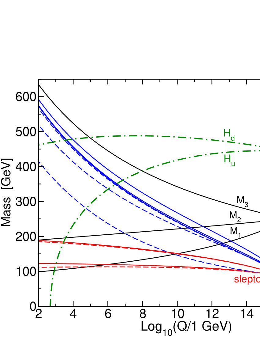
Figure 1.1: Running superpartner masses (from [2]).

In figure 1.1, $\mu$ is the coefficient of the $\mu$-term in the superpotential, coupling the two Higgs $\mu H_{u}H_{d}$. $M_{3}$, $M_{2}$ and $M_{1}$ are the gaugino masses (corresponding to the $SU(3)_{C}$, $SU(2)_{L}$ and $U(1)_{Y}$ gauge groups respectively) running from the common fermion mass $m_{1/2}$. The dashed lines correspond to the third generation sfermions, and the solid lines to the other sfermions, all running from the common scalar mass $m_{0}$. Note that the strong interaction radiative corrections dominate, driving the gluinos and the squarks considerably heavier than the other gauginos and sleptons, and note also that the third generation sfermions are respectively lighter (particularly the stop and the sbottom) as they receive stronger Yukawa (negative) contributions.

Figure 1.1 displays another desirable feature of SUSY models - the Higgs mass (of $H_{u}$) can be driven negative at low $Q$, with the negative Yukawa contributions (largely due to coupling to the top quark) dominating over the gauge contributions and triggering a non-vanishing vacuum expectation value for $H_{u}$ that breaks electroweak symmetry. This mechanism was proposed originally in [3, 4, 5] and a recent review can be found in [6].

Another very compelling reason for low energy SUSY to exist in nature is the apparent unification of coupling strengths. In the Standard Model the couplings don’t quite unify (dashed lines in figure 1.2). However, with the introduction of the superpartners at the previously discussed SUSY scale $M_{SUSY}$ of around $1000$ GeV, the evolution is changed and the three couplings run together, as shown by the solid lines of figure 1.2 (note that the unification scale in figure 1.2 motivates the boundary conditions in figure 1.1). In figure 1.2, the strong coupling represented by $\alpha_{3}(m_{Z})$ is varied from $0.113$ to $0.123$ and the mass thresholds are varied between $250$ and $1000$ GeV. Clearly, if $M_{SUSY}$ had been of a different order of magnitude, the couplings wouldn’t run together: enticingly, introducing SUSY at the scale that leads to gauge coupling unification also solves the hierarchy problem.

Figure 1.2: Running coupling constants (from [2]).

$\alpha_{3}$, $\alpha_{2}$ and $\alpha_{1}$ are the hyperfine constants ($\alpha_{a}=g_{a}^{2}/4\pi$) associated with $SU(3)_{C}$, $SU(2)_{L}$ ($g_{2}=g$ of subsection 1.2.1) and $U(1)_{Y}$ - although note $g_{1}=\sqrt{5/3}g^{\prime}$ (the $g^{\prime}$ of subsection 1.2.1) is normalised in order to be the coefficient in the canonical covariant derivative of $SU(5)$ or $SO(10)$ GUT embeddings of the Standard Model gauge group.

A much more detailed review of SUSY can be found in [2].

1.2.3 Grand Unified Theories

Quarks and leptons share several properties, pointing towards the interesting hypothesis that there might be some underlying fermion unification at some high energy scale $M_{GUT}$ (the unification scale). Just as the Standard Model $SU(2)_{L}$ relates electrons and neutrinos, larger symmetries can relate quarks and leptons. Extending the Standard Model group to the Pati-Salam group $SU(4)_{C}\times SU(2)_{L}\times SU(2)_{R}$ [7] is one example of a GUT that ties quarks and leptons together: the leptons are seen as the extra “colour” of $SU(4)_{C}$. The $SU(2)_{R}$ factor makes the Pati-Salam GUT left-right symmetric. Each of the three families now has one left-handed multiplet including the respective quark and lepton doublets $(Q,L)$, and one right-handed multiplet $(Q^{c},L^{c})$ including the charge conjugates of the right-handed states that now belong to their own doublets ($Q^{c}$ and $L^{c}$). The full symmetry assignments of fermions under the Pati-Salam group are in table 1.2, where the quantum number simplification is readily apparent (particularly when compared with the relatively strange hypercharge assignments of table 1.1).

Field	$SU(4)_{C}$	$SU(2)_{L}$	$SU(2)_{R}$
$(Q,L)$	$\mathbf{4}$	$\mathbf{2}$	$\mathbf{1}$
$(Q^{c},L^{c})$	$\mathbf{\bar{4}}$	$\mathbf{1}$	$\mathbf{\bar{2}}$

Table 1.2: Assignment of fermions under Pati-Salam GUT.

From the multiplet structure in table 1.2 one may see that $\nu^{c}$ is now naturally introduced together with the charge conjugates of the right-handed charged leptons, $e^{c}$ (unlike in the Standard Model).

Although with Pati-Salam there was some extent of fermion unification, the gauge couplings remain independent parameters. To obtain gauge coupling unification at the unification scale $M_{GUT}$ (see figure 1.2), one can instead extend the Standard Model gauge group into a single, simple group (simple in the group theory sense). This is possible as long as the rank of the group is larger or equal than the (combined) rank of the Standard Model gauge group. A commonly utilised example of such a group is $SU(5)$ [8]. Although we won’t go into the details, in $SU(5)$ GUTs the fermions aren’t fully unified, in the sense that they are introduced as two distinct irreducible representations like in Pati-Salam. Despite the appeal of gauge coupling unification, in terms of fermions $SU(5)$ is arguably less appealing than Pati-Salam is: the representations are a $\mathbf{10}$ containing $Q$, $u^{c}$ and $e^{c}$ and a $\bar{\mathbf{5}}$ containing $d^{c}$ and $L$ (note the absence of $\nu^{c}$, which can however be introduced as a singlet just like in the Standard Model).

If one is willing to go further one can extend the symmetry to $SO(10)$. With $SO(10)$ there is not only gauge coupling unification, but enticingly, every fermion of one family fits in one single fundamental representation: the $\mathbf{16}$ of $SO(10)$ (the charge conjugates of the right-handed fermions fit together with the left-handed fermions, including $\nu^{c}$ that nicely completes the multiplet). Another interesting point to note is that $SO(10)$ has as subgroups both Pati-Salam and $SU(5)$, and has inequivalent maximal breaking patterns into one or the other: $SO(10)\rightarrow SU(4)_{C}\times SU(2)_{L}\times SU(2)_{R}$ or $SO(10)\rightarrow SU(5)\times U(1)_{X}$. See for example [1] for a more complete review.

In any of the GUTs discussed, however, the existence of three families remains unexplained. A possible explanation for the families arises from string theories, where the number of families can be related to the geometry of the extra dimensions in some way. In terms of quantum field theories, the more conservative explanation lies in extending the symmetry content with an additional family symmetry acting on the generations.

1.2.4 Neutrino oscillations and data

Neutrino oscillation data implies the existence of neutrino masses. The associated parameters are an important part of the puzzle of fermion masses and mixings, as the existence of neutrino masses leads to leptonic mixing. Neutrino oscillations arise from a straightforward quantum mechanical phenomenon that occurs during the propagation of the neutrinos, causing them to change flavour. This is possible due to the existence of lepton mixing, which is entirely analogous to quark mixing (although the values of the mixing angles are quite different). Instead of the Cabibbo-Kobayashi-Maskawa (CKM) matrix of the quark sector, the respective mixing matrix is sometimes denoted as the Pontecorvo-Maki-Nakagawa-Sakata (PMNS, or often only MNS) matrix. In the basis where the charged lepton mass matrix is diagonal:

$$\nu_{i}=\sum_{\alpha}U_{\alpha i}\nu_{\alpha}$$ (1.5)

$\nu_{i}$ are the mass eigenstates, $\nu_{\alpha}$ the flavour eigenstates. The unitary matrix $U$ expressing the linear combination in eq.(1.5) is the PMNS matrix (here we use Greek letters to clearly distinguish the flavour indices $\alpha$, $\beta$ from the mass indices $i$, $j$). With this it is easy to understand how a specific flavour eigenstate can oscillate to a different one as it propagates: it is composed of a linear combination of mass eigenstates with masses $m_{i}$. The proportion of mass eigenstates will change during the propagation due to the phase factors $e^{-im_{i}\tau}$ in the $\nu_{i}$ rest frame. In the laboratory frame, the phase factor becomes $e^{-i(E_{i}t-p_{i}L)}$ ($E_{i}$ and $p_{i}$ being the energy and momentum of $\nu_{i}$, $t$ and $L$ the time and position, all quantities in the laboratory frame). The neutrinos are very light, with $m_{i}\ll p_{i}$, so one can take $t\simeq L$ (natural units). Furthermore, considering that a specific neutrino flavour $\nu_{\alpha}$ is produced with definite momentum $p$, we have $E_{i}=\sqrt{p^{2}+m_{i}^{2}}\simeq p+m_{i}^{2}/2p$ to good approximation. The phase factor becomes (approximately) $e^{-i(m_{i}^{2}/2p)L}$, and considering the average energy of the various mass eigenstates $E\simeq p$, we can obtain the formula for probability of flavour change from flavour state $\alpha$ into flavour state $\beta$ after propagation for a distance $L$ in the vacuum:

$$P_{\alpha\rightarrow\beta}=\left|\sum_{i}U_{\alpha i}^{\ast}U_{\beta i}e^{-i\frac{m_{i}^{2}L}{2E}}\right|^{2}$$ (1.6)

Eq.(1.6) may be conveniently expressed as $P_{\alpha\rightarrow\beta}=\delta_{\alpha\beta}+Q_{\alpha\beta}$, with $Q_{\alpha\rightarrow\beta}$ being:

$$Q_{\alpha\rightarrow\beta}=-4\sum_{i>j}\mathrm{Re}\left(U_{\alpha i}^{\ast}U_{\beta i}U_{\alpha j}U_{\beta j}^{\ast}\right)\sin^{2}\left(\frac{\Delta m_{ij}^{2}L}{4E}\right)+2\mathrm{Im}\left(U_{\alpha i}^{\ast}U_{\beta i}U_{\alpha j}U_{\beta j}^{\ast}\right)\sin\left(\frac{\Delta m_{ij}^{2}L}{2E}\right)$$ (1.7)

$\mathrm{Re}$ stands for real part and $\mathrm{Im}$ for imaginary part. The terms in eq.(1.7) clearly show that the squared mass differences $\Delta m_{ij}^{2}\equiv m_{i}^{2}-m_{j}^{2}$ are measurable from oscillation (although the overall mass scale isn’t). For a more careful derivation or further details, see for example the original treatment in [9], or the neutrino mixing review in [1] which includes extensive references.

A convenient summary of the neutrino oscillation data is given in [10]. For ease of reference, we reproduce here the relevant table with the values (updated in June 2006 [10]).

parameter	best fit	2$\sigma$	3$\sigma$	4$\sigma$
$\Delta m^{2}_{21}[10^{-5}\mathrm{eV}]$	7.9	7.3–8.5	7.1–8.9	6.8–9.3
$\Delta m^{2}_{31}[10^{-3}\mathrm{eV}]$	2.6	2.2–3.0	2.0–3.2	1.8–3.5
$\sin^{2}\theta_{12}$	0.30	0.26–0.36	0.24–0.40	0.22–0.44
$\sin^{2}\theta_{23}$	0.50	0.38–0.63	0.34–0.68	0.31–0.71
$\sin^{2}\theta_{13}$	0.000	$\leq$ 0.025	$\leq$ 0.040	$\leq$ 0.058

Table 1.3: Neutrino data: best-fit values, 2$\sigma$, 3$\sigma$, and 4$\sigma$ intervals (from [10]).

From [10], the angles of table 1.3 refer to the standard Particle Data Group [1] parametrisation of the unitary mixing matrix:

$$U=\left(\begin{array}[]{ccc}c_{12}c_{13}&s_{12}c_{13}&s_{13}e^{-i\delta_{13}}\\ -s_{12}c_{23}-c_{12}s_{23}s_{13}e^{i\delta_{13}}&c_{12}c_{23}-s_{12}s_{23}s_{13}e^{i\delta_{13}}&s_{23}c_{13}\\ s_{12}s_{23}-c_{12}c_{23}s_{13}e^{i\delta_{13}}&-c_{12}s_{23}-s_{12}c_{23}s_{13}e^{i\delta_{13}}&c_{23}c_{13}\end{array}\right)$$ (1.8)

$c_{ij}\equiv\cos\theta_{ij}$ and $s_{ij}\equiv\sin\theta_{ij}$ (furthermore, $\theta_{12}$ is the solar angle $\theta_{\odot}$, $\theta_{23}$ is the atmospheric angle $\theta_{@}$ and $\theta_{13}$ is the reactor angle). $\delta_{13}$ is a CP-violating phase that hasn’t been measured yet, and we didn’t include here the Majorana phases (usually denoted as $\alpha_{1}$ and $\alpha_{2}$), which only have physical consequences if the neutrinos are Majorana.

It is important to note that the large angles of table 1.3 contrast with the small angles of the CKM matrix (the largest of which, the Cabibbo angle, has $\sin(\theta_{C})<0.23$). The angles are very close to (and consistent with) the special tri-bi-maximal mixing values [11, 12, 13, 14, 15, 16]:

$$s_{12_{TBM}}^{2}=\frac{1}{3}$$ (1.9)

$$s_{23_{TBM}}^{2}=\frac{1}{2}$$ (1.10)

$$s_{13_{TBM}}^{2}=0$$ (1.11)

The experimental data is conveniently displayed in a graphical manner by use of coloured or shaded bars, as in [17], [18]. Figure 1.3 features the two possible mass hierarchies (due to the ambiguity in the sign of the atmospheric squared mass difference), and shows the peculiar situation described by tri-bi-maximal mixing quite clearly: one neutrino mass eigenstate ($\nu_{3}$) is approximately comprised of equal parts $\nu_{\mu}$ and $\nu_{\tau}$, and another ($\nu_{2}$) is approximately equal parts of all three flavour eigenstates.

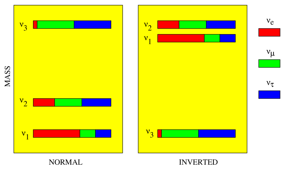
Figure 1.3: Neutrino mixing summary (from [19]).

1.3 Family symmetry review

Including $\nu^{c}$, $U(3)^{6}$ is the largest family symmetry that commutes with the Standard Model gauge group in the absence of the mass terms, the maximum possible symmetry preserved by the kinetic terms. The $U(3)^{6}$ corresponds to one independent $U(3)_{f}$ family symmetry for each of the listed families: the left-handed quark doublet $Q$, the quark singlets $u^{c}$, $d^{c}$; the left-handed lepton doublet $L$, and the lepton singlets $\nu^{c}$, $e^{c}$. If the family symmetry is to commute also with an underlying GUT, then the maximum possible family symmetry is reduced. With an $SO(10)$ GUT, all the families of the Standard Model belong to the same fundamental representation, thus reducing the family symmetry that commutes with the gauge group to a single $U(3)_{f}$.

Any family symmetry that is introduced has to be broken in order to be consistent with the observed fermion masses and mixings - the breaking is thus required by the Yukawa Lagrangian (eq.(1.3)). We designate the fields that break the family symmetry as “flavons”, due to their connection to flavour . Because the family symmetry is not broken by the gauge interactions, which treat each member of the same family equally, the gauge interactions may be said to be “family blind”.

In subsection 1.3.1 we present an incomplete list of recent family symmetry papers, and to conclude the family symmetry review, we provide a very simple family symmetry example in subsection 1.3.2. We use the example to illustrate the general framework, in particular showing that the breaking of the family symmetry leads directly to the fermion masses and mixings. The example is also used to motivate the Froggatt-Nielsen mechanism [20].

1.3.1 Recent models

With the intention of giving a flavour of the topics related to family symmetries, we present a short (and incomplete) list of thirteen recent papers containing “family symmetry” in their title.

We start the review of recent models with the discussion of the paper about models based in Abelian groups. The remaining are all about models based on non-Abelian groups, the proportion perhaps hinting that non-Abelian groups are currently more in favour than Abelian ones. [21] studies properties of the models of [22], based on the Abelian groups $Z_{2}$ and $Z_{4}$.

We now turn to the papers based on non-Abelian family symmetries, starting with the continuous models. [23, 24] both use $SU(3)_{1}\otimes SU(3)_{2}$: [24] is a small extension of [23] (which in turn extended [25] in order to include leptons). We have then the $SO(3)$ model [26], a model with emphasis put in having simple Yukawa operators (each of the leading operators have just a single flavon insertion) - the simplicity then allows the study of details of the messenger sector.

[27, 28, 29] rely on an $A_{4}$ family symmetry. $A_{4}$ has been widely used as a family symmetry: it is a very small subgroup of $SU(3)$ that has a “triplet” representation, very convenient to explain three families ($A_{4}$ is featured in section 3.2 under the guise of $\Delta(12)$, so refer to that section for more details).

The remaining papers are based on discrete non-Abelian family symmetries that are not so commonly used and may be less familiar. We won’t go into details of the groups used in each paper, although we note that they are all (directly or indirectly) subgroups of $SU(3)$. Two of the papers, [30, 31], use $\Sigma(81)$, a subgroup of $SU(3)$: [31] extends [30] in order to obtain tri-bi-maximal mixing. We have also [32] based on $D(6)$, a subgroup of $SO(3)$, and [33] based on $Q_{6}$, a subgroup of $SU(2)$ (and as both $SO(3)$ and $SU(2)$ are continuous subgroups of $SU(3)$, it then follows that $D(6)$ and $Q_{6}$ are discrete subgroups of $SU(3)$).

For the discussion of the last two non-Abelian family symmetry models [34, 35], we add again the $A_{4}$ model of [29], as it shares a common feature with them. [34] is the original paper presenting the $\Delta(27)$ family symmetry model discussed in full detail in section 3.3. [29] uses its $A_{4}$ family symmetry as a subgroup of $SO(3)$ similarly to how $\Delta(27)$ is implemented as a subgroup of $SU(3)_{f}$ in [34] (see chapter 2 and chapter 3). In turn, [35] uses as family symmetry $Z_{7}\rtimes Z_{3}$ - a discrete subgroup of $SU(3)$ only slightly smaller than $\Delta(27)$ (in terms of number of elements - 21 as opposed to 27 - and consequently slightly larger than $\Delta(27)$ in number of allowed invariants). The link connecting the papers is their vacuum expectation value alignment mechanism - both [29] and [35] rely on a vacuum expectation value alignment mechanism similar to the one introduced in [34] - using quartic terms arising from $D$-terms (see subsection 3.3.2 for details). Further, as the group $Z_{7}\rtimes Z_{3}$ shares the same relevant allowed invariants with $\Delta(27)$, the vacuum expectation value alignment mechanism of the two models can actually be identical.

1.3.2 A simple $U(1)_{f}$ toy model

In this supersymmetric toy model we introduce a $U(1)_{f}$ family symmetry commuting with the Standard Model gauge group. We introduce only one flavon field $\phi$, charged under $U(1)_{f}$. $\phi$ will acquire a non-vanishing vacuum expectation value $\langle\phi\rangle$ (through an unspecified mechanism), thus breaking the family symmetry.

We will concentrate solely on the three generations of down-type quarks (for simplicity). The three generations of down quarks are represented as $d_{i}$ for the left-handed fields and as $d^{c}_{i}$ for the right-handed fields ($i$ is the family index, so for example $d_{2}$ is the left-handed strange quark).

The charges under the family symmetry ($U(1)_{f}$) of the Higgs giving mass to the down quarks ($H_{d}$), of the down quarks ($d_{i}$, $d^{c}_{i}$) and of the flavon ($\phi$) are shown in table 1.4.

Field	$U(1)_{f}$
$H_{d}$	$\mathbf{0}$
$\phi$	$-\mathbf{1}$
$d_{1}$	$\mathbf{2}$
$d_{2}$	$\mathbf{1}$
$d_{3}$	$\mathbf{0}$
$d^{c}_{1}$	$\mathbf{2}$
$d^{c}_{2}$	$\mathbf{1}$
$d^{c}_{3}$	$\mathbf{0}$

Table 1.4: $U(1)_{f}$ charge assignments.

Due to the family symmetry, nearly all the gauge invariant mass terms require inclusion of some power of the flavon field $\phi$ (this is comparable to how all Dirac mass terms must include $H$ to be invariant under $SU(2)_{L}$). It is straightforward to obtain the effective Yukawa superpotential for the down type quarks:

$$P_{d}=d_{3}d^{c}_{3}H+\frac{\phi}{M}d_{3}d^{c}_{2}H+\frac{\phi}{M}d_{2}d^{c}_{3}H$$ (1.12)

$$+\left(\frac{\phi}{M}\right)^{2}d_{2}d^{c}_{2}H+\left(\frac{\phi}{M}\right)^{3}d_{2}d^{c}_{1}H+\left(\frac{\phi}{M}\right)^{3}d_{1}d^{c}_{2}H$$ (1.13)

$$+\left(\frac{\phi}{M}\right)^{4}d_{1}d^{c}_{1}H+\left(\frac{\phi}{M}\right)^{2}d_{1}d^{c}_{3}H+\left(\frac{\phi}{M}\right)^{2}d_{3}d^{c}_{1}H$$ (1.14)

The first term of eq.(1.12) generates $(M^{d})_{33}$ - effectively the bottom mass (there are sub-leading corrections from the other terms). When $\phi$ acquires its vacuum expectation value $\langle\phi\rangle$, the remaining entries of $M^{d}$ are filled out by increasing powers of the ratio $\frac{\langle\phi\rangle}{M}=\epsilon$. Note the presence of the yet unspecified mass scale $M$. For now we simply take $M$ to be some large mass scale such that $\epsilon$ is a small parameter. The justification lies in considering $M$ to be the mass of a Froggatt-Nielsen messenger as described in more detail in subsection 1.4.1. With small $\epsilon$, we can generate a strong hierarchy in $M^{d}$:

$$M^{d}\propto\left(\begin{array}[]{ccc}\epsilon^{4}&\epsilon^{3}&\epsilon^{2}\\ \epsilon^{3}&\epsilon^{2}&\epsilon\\ \epsilon^{2}&\epsilon&1\end{array}\right)$$ (1.15)

Although very simple (and not phenomenologically viable), this model clearly illustrates the philosophy of using family symmetries together with the Froggatt-Nielsen mechanism (see subsection 1.4.1) to control the fermion masses and mixings (and obtain hierarchies) through expansions of small parameters: the ratio of the flavon vacuum expectation values with superheavy messenger masses (of what will be identified as Froggatt-Nielsen messenger fields in subsection 1.4.1).

1.4 Mass generation mechanisms

1.4.1 Froggatt-Nielsen mechanism

The Froggatt-Nielsen mechanism allows the generation of masses through higher order tree-level diagrams involving superheavy fields: the Froggatt-Nielsen messenger fields [20].

A simple example of the Froggatt-Nielsen mechanism is the diagram in figure 1.4, where the arrows denote the chirality of the fields (like in other diagrams).

Figure 1.4: Simple Froggatt-Nielsen diagram.

The superheavy fields $\bar{A}$, $A$ are the Froggatt-Nielsen messenger fields, and have a mass term $M_{A}\bar{A}A$ (corresponding to the mass insertion represented by “$\times$” in figure 1.4). Note that the messengers must have appropriate Standard Model and family symmetry charge assignments - namely, it is relevant to consider the placement of the $H$ insertion (as it carries $SU(2)_{L}$ charge) and likewise $\phi$ will carry family charge. Consider specifically the generation of $M^{d}_{23}$ in eq.(1.15): it can proceed precisely through a simple Froggatt-Nielsen diagram with just one flavon insertion, with $d_{2}$ and $d_{3}^{c}$ as the external fields. If the ordering of $H$ and $\phi$ are as displayed in figure 1.4, then $A$ must have $U(1)_{f}$ charge $+1$ (and respectively, $\bar{A}$ has $-1$).

When the messengers are integrated out, the superpotential term respective to figure 1.4 becomes:

$$P=\frac{\langle\phi\rangle}{M_{A}}\psi\psi^{c}\langle H\rangle=m_{\psi}\psi\psi^{c}$$ (1.16)

The effective mass is $m_{\psi}\equiv\frac{\langle\phi\rangle}{M_{A}}\langle H\rangle$.

A more general diagram is displayed in figure 1.5, featuring more than one superheavy mass insertion ($\bar{A}$ and $A$, $\bar{B}$ and $B$, $\bar{C}$ and $C$ with mass terms $M_{A}\bar{A}A$, $M_{B}\bar{B}B$, $M_{C}\bar{C}C$ respectively).

Figure 1.5: Generic Froggatt-Nielsen diagram.

The generalisation is simple, but one should note again that the charges of the messengers must be such that the diagram is allowed. In order to consider another specific case, consider for simplicity the following $U(1)_{f}$ charge assignments: $\phi_{1}$ has family charge $-1$, $\phi_{2}$ has $-2$ and $\phi_{3}$ has $+3$, with all other non-messenger fields neutral (note this is not the toy model discussed in subsection 1.3.2). With the ordering of figure 1.5, the charges of the messengers would be $0$, $0$, $1$, $-1$, $+3$ and $-3$ respectively for $\bar{A}$, $A$, $\bar{B}$, $B$, $\bar{C}$ and $C$. The effective superpotential term is invariant as required:

$$P=\frac{\langle\phi_{1}\rangle\langle\phi_{2}\rangle\langle\phi_{3}\rangle}{M_{A}M_{B}M_{C}}\psi\psi^{c}\langle H\rangle$$ (1.17)

Corresponding to an effective mass $m_{\psi}\equiv\frac{\langle\phi_{1}\rangle\langle\phi_{2}\rangle\langle\phi_{3}\rangle}{M_{A}M_{B}M_{C}}\langle H\rangle$.

1.4.2 Seesaw mechanism

The seesaw mechanism [36, 37, 38, 39, 40] is similar to the Froggatt-Nielsen mechanism. It generates effective masses for the light neutrinos by integrating out heavy neutrino states. Figure 1.6 is a typical type I seesaw diagram (with the “$\times$” in the $\nu^{c}$ propagator denoting the Majorana mass insertion).

Figure 1.6: Type I seesaw diagram.

The right-handed neutrino masses (in general, eigenvalues of a mass matrix $M_{M}$) are naturally expected to be much larger than the neutrino Dirac masses (eigenvalues of $M_{D}^{\nu}\propto Y^{\nu}$ of eq.(1.3)). The reason for this is that $\nu^{c}$ are singlets of the Standard Model, and the mass term $M_{M}\nu^{c}\nu^{c}$ is automatically invariant. In other words, $M_{M}$ is not protected by the Standard Model gauge group, unlike $M_{D}^{\nu}$ which is only non-vanishing after $SU(2)_{L}$ is spontaneously broken by $\langle H\rangle$ (see the Yukawa Lagrangian in eq.(1.3)). If indeed the Majorana masses have large values, that enables us to integrate out the $\nu^{c}$ fields and obtain the formula for the effective light neutrino masses approximately given by [41, 42]:

$$M_{\nu}=-(M_{D}^{\nu})(M_{M}^{-1})(M_{D}^{\nu})^{T}$$ (1.18)

The minus sign can be absorbed by redefinition of the fields (it is however relevant if type II seesaw [43, 44] is present).

The general structure of eq.(1.18) can be obtained by considering the simpler one family case. Doing so we clearly obtain the minus sign (although we won’t get the transpose, for obvious reasons). We introduce only one left-handed neutrino, $\nu$ and one right-handed neutrino, $\nu^{c}$. Due to the symmetry of the Standard Model, the $M_{L}\nu\nu$ mass term is not invariant. However, we can have in general a Dirac mass term $M_{D}^{\nu}\nu\nu^{c}$ as well as a Majorana mass term $M_{R}\nu^{c}\nu^{c}$. We can express this as a $2\times 2$ neutrino mass matrix $M^{\nu}$:

$$L=\left(\begin{array}[]{cc}\nu^{\dagger}&\nu^{c\dagger}\end{array}\right)M^{\nu}\left(\begin{array}[]{c}\nu\\ \nu^{c}\end{array}\right)$$ (1.19)

$$M^{\nu}=\left(\begin{array}[]{cc}0&M_{D}^{\nu}\\ M_{D}^{\nu}&M_{R}\end{array}\right)$$ (1.20)

If $M_{D}^{\nu}\ll M_{R}$ (a natural condition, as $M_{R}$ isn’t protected by $SU(2)_{L}$), one can readily identify the approximate eigenvalues of $M^{\nu}$ by using its matrix invariants, namely the determinant $Det\left(M^{\nu}\right)=-\left(M_{D}^{\nu}\right)^{2}$ and the trace $Tr\left(M^{\nu}\right)=M_{R}$. The largest eigenvalue must then be approximately $M_{R}$ (keeping the trace invariant), and the smallest eigenvalue must then be $-\left(M_{D}^{\nu}\right)^{2}/M_{R}$ to preserve the determinant: this is precisely the result one gets from eq.(1.18) applied to the particular case of one generation of each type of neutrino. The exact eigenvalues in this one generation case are:

$$M^{\nu}_{+}=\frac{1}{2}\left(M_{R}+\sqrt{M_{R}^{2}+4\left(M_{D}^{\nu}\right)^{2}}\right)$$ (1.21)

$$M^{\nu}_{-}=\frac{1}{2}\left(M_{R}-\sqrt{M_{R}^{2}+4\left(M_{D}^{\nu}\right)^{2}}\right)$$ (1.22)

By expanding the square root we verify that the approximate values obtained based on the matrix invariants are indeed correct to leading order. Generalising to three generations of each type of neutrino, we obtain eq.(1.18), where $M_{D}^{\nu}$ and $M_{R}$ are now $3\times 3$ matrices.

We can also intuitively understand eq.(1.18) by inspection of figure 1.6, now with the three generations and using the appropriate mass matrices. When $H$ acquires the vacuum expectation value $\langle H\rangle=h$, the vertex on the left becomes a neutrino Dirac mass matrix proportional to $h$, corresponding to $M_{D}^{\nu}$: the mass term is $M_{D}^{\nu}\nu\nu^{c}$, suppressing the family indices. The mass insertion is the Majorana mass matrix $M_{M}$ of the $\nu^{c}$ fields: the mass term is $M_{M}\nu^{c}\nu^{c}$, suppressing the family indices. The right-handed neutrino propagates in the internal line and by integrating it out we get the inverse matrix, $M_{M}^{-1}$. Finally the vertex on the right likewise corresponds to $\left(M_{D}^{\nu}\right)^{T}$ (the transpose due to the inverted ordering), and the resulting $M_{\nu}$ mass matrix for the effective neutrinos is proportional to $h^{2}$.

Although we make no use of it in the following chapters, we note for completeness the existence of the type II seesaw mechanism [43, 44], requiring an $SU(2)_{L}$ triplet Higgs $\Delta$, of which a typical diagram is shown in figure 1.7.

Figure 1.7: Type II seesaw diagram.

If the type II seesaw is present in a model and the contribution can’t be neglected, an extra term $M_{L}$ must be added to the seesaw formula in eq.(1.18):

$$M_{\nu}=M_{L}-(M_{D}^{\nu})(M_{M}^{-1})(M_{D}^{\nu})^{T}$$ (1.23)

Note that now the minus sign is relevant, and indeed due to the presence of $M_{L}$ one can’t freely redefine the fields any longer (the relative sign between type I and type II terms is important). $M_{L}$ occupies the formerly vanishing top left quadrant: the left-left quadrant of the neutrino matrix $M^{\nu}$ (hence the subscript $L$ in $M_{L}$). Again taking the simpler example of one family of each neutrino type (left-handed and right-handed), $M_{L}$ occupies the $11$ entry of the $2\times 2$ matrix (where there used to be a zero):

$$M^{\nu}=\left(\begin{array}[]{cc}M_{L}&M_{D}^{\nu}\\ M_{D}^{\nu}&M_{R}\end{array}\right)$$ (1.24)

Refer for example to [41, 42] for detailed reviews of neutrino physics.

Chapter 2 Continuous family symmetries

2.1 Framework and outline

As discussed in section 1.1, explaining the observed pattern of quark and lepton masses and mixing angles remains a central issue in our attempt to construct a theory beyond the Standard Model. Perhaps the most conservative possible explanation is that the symmetry of the Standard Model is extended to include a family symmetry which orders the Yukawa couplings responsible for the mass matrix structure. In this chapter, we consider this possibility, presenting as example a specific model with a continuous $SU(3)_{f}$ family symmetry [45]. In this section we begin to establish the framework introduced in [45], used not only in the continuous family symmetry model of this chapter, but also used for models based in discrete family symmetries (presented in chapter 3).

If one restricts the discussion to the quark sector it is possible to build quite elegant examples involving a spontaneously broken family symmetry which generates the observed hierarchical structure of quark masses and mixing angles. However, attempts to extend this to the leptons has proved very difficult, mainly because the large mixing angles needed to explain neutrino oscillation contrast with the small mixing angles observed in the quark sector. As established in subsection 1.2.4, the present experimental values for lepton mixing are consistent and actually well described by the Harrison, Perkins and Scott “tri-bi-maximal mixing” scheme [11, 12, 13, 14, 15, 16] in which the atmospheric neutrino mixing angle is maximal ($\sin^{2}(\theta_{@})=1/2)$ and the solar neutrino mixing is “tri-maximal” ($\sin^{2}(\theta_{\odot})=1/3$), which corresponds to the PMNS leptonic mixing matrix taking the following special form:

$$U_{PMNS}\propto\left[\begin{array}[]{ccc}-\sqrt{\frac{2}{6}}&\sqrt{\frac{1}{3}}&0\\ \sqrt{\frac{1}{6}}&\sqrt{\frac{1}{3}}&\sqrt{\frac{1}{2}}\\ \sqrt{\frac{1}{6}}&\sqrt{\frac{1}{3}}&-\sqrt{\frac{1}{2}}\end{array}\right]$$ (2.1)

If the mixing is indeed very close to tri-bi-maximal mixing, it represents a strong indication that an existing family symmetry should be non-Abelian to be able to relate the magnitude of the Yukawa couplings of different families (something an Abelian symmetry cannot do). Several models based on non-Abelian symmetries have been constructed that account for this structure of leptonic mixing (examples include [46, 47, 48, 49, 50]). It is possible to construct models in a different class, where the underlying family symmetry provides a full description of the complete fermionic structure (e.g. [51, 52]) - see [41, 42] or [53, 54, 55, 56] for review papers with extensive references of both types of models. In models describing not just the leptons, the family symmetry explains also why the quarks have a strongly hierarchical structure with small mixing (in contrast to the large leptonic mixing), and the Yukawa coupling matrices at the GUT scale take the form given by fits to the data [57, 58]:

$$Y^{u}\propto\left(\begin{array}[]{ccc}0&i\,\epsilon_{u}^{3}&\epsilon_{u}^{3}\cr\cdot&\epsilon_{u}^{2}&\epsilon_{u}^{2}\cr\cdot&\cdot&1\end{array}\right)$$ (2.2)

$$Y^{d}\propto\left(\begin{array}[]{ccc}0&1.7\epsilon_{d}^{3}&(0.8)e^{-i\,(45)^{o}}\epsilon_{d}^{3}\cr\cdot&\epsilon_{d}^{2}&{(2.1)}\epsilon_{d}^{2}\cr\cdot&\cdot&1\end{array}\right)$$ (2.3)

The expansion parameters are:

$$\epsilon_{d}\simeq{0.13},\epsilon_{u}\simeq 0.048$$ (2.4)

Following [58], we represent the Yukawa matrices in the $\overline{MS}$ scheme below the $Z^{0}$ mass $M_{Z}$, and in the $\overline{DR}$ scheme above $M_{Z}$.

In this chapter, we consider in detail how the hierarchical quark structures together with lepton tri-bi-maximal mixing can emerge in theories with an $SU(3)_{f}$ family symmetry (and in chapter 3, how those can emerge in theories with non-Abelian discrete subgroups of $SU(3)_{f}$).

The use of $SU(3)_{f}$ is of particular interest: $U(3)$ is the largest family symmetry that commutes with $SO(10)$ and thus one can fit the family symmetry group together with promising GUT extensions of the Standard Model. We consider this to be a desirable feature of a complete model of quark and lepton masses and mixing angles, and choose to include an $SO(10)$ symmetry, aiming to preserve the respective phenomenologically successful GUT relations between quark and lepton masses. To do so, we require that the models be consistent with the underlying unified structure, either at the field theory level or at the level of the superstring. This requirement is very constraining because all the left-handed  members of a single family must have the same family charge (or multiplet assignments). Despite these strong constraints, it is possible to build models capable of describing all quark and lepton masses and mixing angles, featuring tri-bi-maximal mixing in the lepton sector. Due to the GUT, there is a close relation between quark and lepton masses, and the Georgi-Jarlskog relations between charged lepton and down-type quark masses [59] are obtained. Likewise, the symmetric structure of the mass matrices is motivated by the $SO(10)$ GUT, reproducing the phenomenologically successful Gatto-Sartori-Tonin relation [60] for the $(1,2)$ sector mixing:

$$\left|V_{us}\right|=\left|\sqrt{\frac{m_{d}}{m_{s}}}-e^{i\phi_{1}}\sqrt{\frac{m_{u}}{m_{c}}}\right|$$ (2.5)

The phase $\phi_{1}$ can be in some cases a good approximation to the CKM complex phase $\delta$, as discussed in [58] (see also [57]).We note for completeness that the corrections induced by the two schemes used ($\overline{MS}$ scheme below $M_{Z}$ and $\overline{DR}$ scheme above) is smaller than the accuracy of the Gatto-Sartori-Tonin relation.

Finally, because the charged lepton structure is related to down quark structure, it is possible to relate the quark mixing angles with the predicted deviations of leptonic mixing from the tri-bi-maximal (neutrino mixing) values [61, 62].

By itself, such a unified implementation of $SU(3)_{f}$ does not explain why the mixing angles are small in the quark sector while they are large in the lepton sector. If these contrasting observations are to be consistent with a spontaneously broken family symmetry there must be a mismatch between the symmetry breaking pattern in the quark and charged lepton sectors and the symmetry breaking pattern in the neutrino sector. In the quark sector and charged lepton sectors the first stage of family symmetry breaking, $SU(3)_{f}\rightarrow SU(2)_{f}$, generates the third generation masses while the remaining masses are only generated by the second stage of breaking of the residual $SU(2)_{f}$. However, in the neutrino mass sector the dominating breaking must be rotated by $\pi/4$ relative to this, so that an equal combination of $\nu_{\tau}$ and $\nu_{\mu}$ receives mass at the first stage of mass generation. The subsequent breaking generating the light masses must be misaligned by approximately the tri-maximal angle in order to describe solar neutrino oscillation ($\sin^{2}(\theta_{\odot})=1/3$).

One can obtain tri-bi-maximal mixing through the effective Lagrangian:

$$L_{\nu}=\lambda_{@}(\nu_{\mu}-\nu_{\tau})^{2}+\lambda_{\odot}(\nu_{e}+\nu_{\mu}+\nu_{\tau})^{2}$$ (2.6)

$\lambda_{@}$ and $\lambda_{\odot}$ need to have the appropriate values (to account for the observed mass squared differences). This Lagrangian represents a normal hierarchy scheme of $m_{1}<m_{2}<m_{3}$ (see figure 1.3) where the lightest neutrino mass eigenstate is approximately massless ($m_{1}\simeq 0$, and thus its term is not shown in eq.(2.6)). In this case, the masses are given to good approximation by taking the square root of the squared mass differences: $\lambda_{@,\odot}=\sqrt{\Delta m^{2}_{@,\odot}}$. The effective Lagrangian in eq.(2.6) clearly shows the solar and atmospheric eigenstates feature tri-bi-maximal mixing.

The main difficulty in realising tri-bi-maximal mixing in this class of models with underlying unification is the need to explain why the dominant breaking leading to the generation of third generation masses in the quark sector is not also the dominant effect in the neutrino sector. At first sight it appears quite unnatural. However, if neutrino masses are generated by the seesaw mechanism (see subsection 1.4.2) this difficulty can be overcome, and one can obtain neutrino tri-bi-maximal mixing as shown in eq.(2.6) even if all quark and lepton Dirac mass matrices, including those of the neutrinos, have similar forms up to Georgi-Jarlskog type factors. To see this consider the form of the seesaw mechanism (neglecting here the minus sign of eq.(1.18)):

$$M_{\nu}=(M_{D}^{\nu})(M_{M}^{-1})(M_{D}^{\nu})^{T}$$ (2.7)

As in subsection 1.4.2, $M_{\nu}$ is the effective mass matrix for the light neutrino states coupling $\nu$ to $\nu$, $M_{D}^{\nu}$ is the Dirac mass matrix coupling $\nu$ to $\nu^{c}$ and $M_{M}$ is the Majorana mass matrix coupling $\nu^{c}$ to $\nu^{c}$. We consider the case where the Majorana mass matrix has an hierarchical structure of the form:

$$M_{M}\simeq\left({{\begin{array}[]{*{20}c}{M_{1}\hfill}&\hfill\hfil&\hfill\hfil\\ \hfill\hfil&{M_{2}\hfill}&\hfill\hfil\\ \hfill\hfil&\hfill\hfil&{M_{3}\hfill}\\ \end{array}}}\right)\quad M_{1}<<M_{2}<<M_{3}.$$ (2.8)

For a sufficiently strong hierarchy this gives rise to sequential domination [63, 64, 65, 66, 67, 68]: the heaviest of the three light eigenstates gets its mass from the exchange of the lightest (right-handed) singlet neutrino with Majorana mass $M_{1}$. In this case the contribution to the light neutrino mass matrix of the field responsible for the dominant terms in the Dirac mass matrix, $(M^{\nu}_{D})_{33}$, is suppressed by the relative factor $M_{2}/M_{3}$ (or $M_{1}/M_{3}$) and can readily be sub-dominant in the neutrino sector. The key point is that any underlying quark-lepton symmetry is necessarily broken in the neutrino sector due to the Majorana masses of the right-handed neutrino states and, through the seesaw mechanism, this feeds into the neutrino masses and the lepton mixing angles. The simpler case where we take the Majorana masses in the diagonal basis clearly illustrates how this effect can hide an existing quark-lepton symmetry in the Dirac mass sector.

In the $SU(3)_{f}$ model detailed in this chapter (and in the models of chapter 3) we implement this structure to achieve near tri-bi-maximal mixing for the leptons. We consider only the case of supersymmetric extensions of the Standard Model, because we rely on SUSY to keep the hierarchy problem associated with a high-scale GUT under control. Rather than work with a complete $SO(10)\otimes G_{f}$ theory (which, in a string theory, may only be relevant above the string scale) we consider here the case where the gauge symmetry is $G_{PS}\otimes G_{f}$ where $G_{PS}$ is the Pati-Salam group $G_{PS}\equiv SU(4)_{PS}\otimes SU(2)_{L}\otimes SU(2)_{R}$ described in subsection 1.2.3. The $G_{f}$ representation assignments are chosen in a way consistent with this being a subgroup of $SO(10)\otimes G_{f}$. The construction of the models closely follows that of [69] and [70], and we proceed by identifying simple auxiliary symmetries capable of restricting the allowed Yukawa couplings to give viable mass matrices for the quarks and leptons. For a particular model, we need to pay particular attention to an analysis of the scalar potential which is ultimately responsible for the vacuum alignment generating tri-bi-maximal mixing.

The Majorana mass matrices are generated by the lepton number violating sector. To fulfil the suppression of the otherwise dominant contribution arising from the Dirac masses, $(M^{\nu}_{D})_{33}$, the dominant contribution to the Majorana mass matrix for the neutrinos is also going to be aligned along the $3$rd direction (as is also the case for all the fermion Dirac matrices). We will show that by doing so, it is possible to achieve tri-bi-maximal mixing very closely, with the small (but significant) deviations coming from the charged lepton sector. This type of situation is described in some detail in [61, 62].

In section 2.2, we present the specific charge assignments of the continuous model, continuing to outline the general strategy that is implemented not only in the continuous model featured in this chapter but also in the discrete models of chapter 3. The respective spontaneous symmetry breaking discussion is presented in subsection 2.3. Subsection 2.4 features the leading superpotential terms generating the fermions masses as well as the discussion of the messenger sector - features which are going to be used (with small changes) also in chapter 3. The phenomenology of the continuous model is presented in subsection 2.5. The summary of the continuous model results, in subsection 2.7, serves also as motivation for the discrete models presented in chapter 3 (namely the $\Delta(27)$ model of section 3.3).

2.2 $SU(3)_{f}$ family symmetry model

As discussed in section 2.1, we keep the assignment of $SU(3)_{f}$ representations consistent with an underlying $SO(10)\otimes G_{f}$ symmetry, even though we will effectively use only the Pati-Salam subgroup of $SO(10)$ in constructing models ($G_{PS}\equiv SU(4)_{PS}\otimes SU(2)_{L}\otimes SU(2)_{R}$). We denote the Standard Model fermions as $\psi_{i}$ and $\psi_{j}^{c}$ (where $i,j=1,2,3$ are family indices). $\psi_{i}$ and $\psi_{i}^{c}$ are assigned to a $(\mathbf{16},\mathbf{3})$ representation of $SO(10)\otimes SU(3)_{f}$. The Higgs doublets of the Standard Model (of which we require two due to SUSY) are part of $(\mathbf{10},\mathbf{1})$ representations, labelled jointly as $H$ for simplicity. In addition we introduce the Higgs $H_{45}$ in the adjoint representation of $SO(10)$, as $(\mathbf{45},\mathbf{1})$. In our effective theory $H_{45}$ has a vacuum expectation value consistent with the residual $G_{PS}\otimes G_{f}$ symmetry which leaves the hypercharge $Y_{k}=kT_{3R}+(B-L)/2$ unbroken, as discussed in [71] (see also [69]; note that the expression we use for $Y_{k}$ differs by an overall multiplicative factor of $2$ from the hypercharge used in those references). $T_{3R}$ is the right isospin associated with $SU(2)_{R}$ (so for example, $T_{3R}(\nu^{c})=+1/2$). Although $Y_{k}$ is the most general expression, the phenomenology of the models requires a factor of magnitude $3$ ($-3$ or $+3$) between the $Y_{k}$ of charged leptons and of down quarks and as such, the possible choices for $k$ are $0$ or $1$ as we will see. We choose $k=1$ so that $Y(\nu^{c})=0$, which will be helpful in separating the neutrino terms from the charged leptons:

$$Y_{k}=kT_{3R}+(B-L)/2$$ (2.9)

$$Y_{k=1}\equiv Y=T_{3R}+(B-L)/2$$ (2.10)

To successfully recover the Standard Model the family symmetry must be completely broken. We will do so in steps, first with a dominant breaking $SU(3)_{f}\rightarrow SU(2)_{f}$, followed by the breaking of the remaining $SU(2)_{f}$. This spontaneous symmetry breaking will be achieved by additional Standard Model singlet scalar fields, which in the models discussed here are typically (but not always) either triplets ($\mathbf{3}_{i}$) or anti-triplets ($\bar{\mathbf{3}}^{i}$) of the family symmetry $SU(3)_{f}$. The alignment of their vacuum expectation values is extremely relevant to the results and is discussed in subsection 2.3 (as well as in more detail in appendix A). To construct a realistic model it is necessary to further extend the symmetry in order to eliminate unwanted terms that would otherwise show up in the effective Lagrangian. The construction of a specific model requires the specification of the full multiplet content together with its transformation properties under $G_{PS}\otimes SU(3)_{f}$ and under the additional symmetry needed to limit the allowed couplings. In the $SU(3)_{f}$ model we consider in this chapter [45], the additional symmetry is $G=R\otimes U(1)\otimes U^{\prime}(1)$. The multiplet content and transformation properties for the model are given in table 2.1. In addition to the fields already discussed, table 2.1 includes the fields $\theta$ and $\bar{\theta}$ whose vacuum expectation values break $SU(4)_{PS}$, breaking also lepton number and thus generating the Majorana masses (as described in subsection 2.4). Table 2.1 also features additional $G_{PS}$ singlet fields required for vacuum expectation value alignment, as discussed in appendix A.

Field	$SU(3)_{f}$	$SU(4)_{PS}$	$SU(2)_{L}$	$SU(2)_{R}$	$R$	$U(1)$	$U(1)^{\prime}$
$\psi$	$\mathbf{3}$	$\mathbf{4}$	$\mathbf{2}$	$\mathbf{1}$	$\mathbf{1}$	$\mathbf{0}$	$\mathbf{0}$
$\psi^{c}$	$\mathbf{3}$	$\bar{\mathbf{4}}$	$\mathbf{1}$	$\bar{\mathbf{2}}$	$\mathbf{1}$	$\mathbf{0}$	$\mathbf{0}$
$\theta$	$\mathbf{3}$	$\bar{\mathbf{4}}$	$\mathbf{1}$	$\bar{\mathbf{2}}$	$\mathbf{0}$	$\mathbf{0}$	$\mathbf{0}$
$\bar{\theta}$	$\bar{\mathbf{3}}$	$\mathbf{4}$	$\mathbf{1}$	$\mathbf{2}$	$\mathbf{0}$	$\mathbf{0}$	$\mathbf{0}$
$H$	$\mathbf{1}$	$\mathbf{1}$	$\mathbf{2}$	$\mathbf{2}$	$\mathbf{0}$	$-\mathbf{4}$	$-\mathbf{4}$
$H_{45}$	$\mathbf{1}$	$\mathbf{15}$	$\mathbf{1}$	$\mathbf{3}$	$\mathbf{0}$	$\mathbf{2}$	$\mathbf{2}$
$\phi_{3}$	$\mathbf{3}$	$\mathbf{1}$	$\mathbf{1}$	$\mathbf{1}$	$\mathbf{0}$	$-\mathbf{2}$	$-\mathbf{3}$
$\bar{\phi}_{3}$	$\mathbf{\bar{3}}$	$\mathbf{1}$	$\mathbf{1}$	$\mathbf{3}\oplus\mathbf{1}$	$\mathbf{0}$	$\mathbf{2}$	$\mathbf{2}$
$\phi_{2}$	$\mathbf{3}$	$\mathbf{1}$	$\mathbf{1}$	$\mathbf{1}$	$\mathbf{0}$	$-\mathbf{1}$	$\mathbf{1}$
$\bar{\phi}_{2}$	$\bar{\mathbf{3}}$	$\mathbf{1}$	$\mathbf{1}$	$\mathbf{1}$	$\mathbf{0}$	$-\mathbf{1}$	$\mathbf{1}$
$\phi_{23}$	$\mathbf{3}$	$\mathbf{1}$	$\mathbf{1}$	$\mathbf{1}$	$\mathbf{0}$	$-\mathbf{4}$	$-\mathbf{3}$
$\bar{\phi}_{23}$	$\bar{\mathbf{3}}$	$\mathbf{1}$	$\mathbf{1}$	$\mathbf{1}$	$\mathbf{0}$	$\mathbf{1}$	$\mathbf{1}$
$\phi_{123}$	$\mathbf{3}$	$\mathbf{1}$	$\mathbf{1}$	$\mathbf{1}$	$\mathbf{0}$	$\mathbf{0}$	$\mathbf{1}$
$\bar{\phi}_{123}$	$\mathbf{\bar{3}}$	$\mathbf{1}$	$\mathbf{1}$	$\mathbf{1}$	$\mathbf{0}$	$\mathbf{3}$	$\mathbf{3}$
$X_{3}$	$\mathbf{1}$	$\mathbf{1}$	$\mathbf{1}$	$\mathbf{1}$	$\mathbf{2}$	$\mathbf{0}$	$\mathbf{1}$
$Y_{2}$	$\mathbf{1}$	$\mathbf{1}$	$\mathbf{1}$	$\mathbf{1}$	$\mathbf{2}$	$-\mathbf{1}$	$-\mathbf{3}$
$X_{23}$	$\mathbf{1}$	$\mathbf{1}$	$\mathbf{1}$	$\mathbf{1}$	$\mathbf{2}$	$\mathbf{1}$	$\mathbf{0}$
$Y_{23}$	$\mathbf{1}$	$\mathbf{1}$	$\mathbf{1}$	$\mathbf{1}$	$\mathbf{2}$	$\mathbf{3}$	$\mathbf{2}$
$X_{123}$	$\mathbf{1}$	$\mathbf{1}$	$\mathbf{1}$	$\mathbf{1}$	$\mathbf{2}$	$-\mathbf{3}$	$-\mathbf{4}$
$Y_{123}$	$\mathbf{1}$	$\mathbf{1}$	$\mathbf{1}$	$\mathbf{1}$	$\mathbf{2}$	$-\mathbf{1}$	$-\mathbf{2}$
$Z_{123}$	$\mathbf{1}$	$\mathbf{1}$	$\mathbf{1}$	$\mathbf{1}$	$\mathbf{4/3}$	$-\mathbf{3}$	$-\mathbf{4}$
$S_{3}$	$\mathbf{1}$	$\mathbf{1}$	$\mathbf{1}$	$\mathbf{1}$	$\mathbf{0}$	$\mathbf{0}$	$-\mathbf{1}$
$\Sigma$	$\mathbf{3}\otimes\bar{\mathbf{3}}$	$\mathbf{1}$	$\mathbf{1}$	$\mathbf{1}$	$\mathbf{2/3}$	$\mathbf{0}$	$\mathbf{0}$

Table 2.1: Field and representation content of continuous model.

2.3 Spontaneous symmetry breaking

We now summarise the pattern of family symmetry breaking in the continuous model. The detailed minimisation of the effective potential which gives this structure is addressed in appendix A.

The dominant breaking of $SU(3)_{f}$ responsible for the third generation quark and charged lepton masses is provided by the $\bar{\phi}_{3}$ vacuum expectation value:

$$\langle\bar{\phi}_{3}\rangle=\left(\begin{array}[]{ccc}0&0&1\end{array}\right)\otimes\left(\begin{array}[]{cc}a_{u}&0\\ 0&a_{d}\end{array}\right)$$ (2.11)

The $SU(3)\times SU(2)_{R}$ structure is explicitly exhibited in eq.(2.11). Note that $\bar{\phi}_{3}$ also breaks $SU(2)_{R}$; at this stage, the residual symmetry is $(SU(4)_{PS}\otimes SU(2)_{L}\otimes U(1)_{R})\otimes SU(2)_{f}$. To preserve $D$-flatness, another field, $\phi_{3}$, also acquires a large vacuum expectation value:

$$\langle\phi_{3}\rangle=\left(\begin{array}[]{c}0\\ 0\\ \sqrt{a_{u}^{2}+a_{d}^{2}}\end{array}\right)$$ (2.12)

The fields $\theta$ and $\bar{\theta}$, responsible for breaking $SU(4)_{PS}$ also acquire vacuum expectation values  along the same direction (see appendix A):

$$\langle\bar{\theta}\rangle\propto\left(\begin{array}[]{ccc}0&0&1\end{array}\right)$$ (2.13)

$$\langle\theta\rangle\propto\left(\begin{array}[]{c}0\\ 0\\ 1\end{array}\right)$$ (2.14)

The breaking of the remaining $SU(2)_{f}$ family symmetry is achieved when a triplet $\phi_{2}$ acquires the vacuum expectation value:

$$\langle\phi_{2}\rangle=\left(\begin{array}[]{c}0\\ y\\ 0\end{array}\right)$$ (2.15)

Due to the allowed couplings in the superpotential (see appendix A) this vacuum expectation value is orthogonal to $\langle\bar{\phi}_{3}\rangle$.

Further fields acquire vacuum expectation values  constrained by the allowed couplings in the theory. As detailed in appendix A the field $\bar{\phi}_{23}$ acquires a vacuum expectation value:

$$\langle\bar{\phi}_{23}\rangle=\left(\begin{array}[]{ccc}0&b&-b\end{array}\right)$$ (2.16)

It is the underlying $SU(3)_{f}$ that forces the vacuum expectation values  in the $2$nd and the $3$rd directions to be equal in magnitude, so that the $\bar{\phi}_{23}$ is rotated by $\pi/4$ relative to the $\bar{\phi}_{3}$ vacuum expectation value. This is important in generating an acceptable pattern for quark masses and in generating bi-maximal mixing in the lepton sector. Finally the fields $\bar{\phi}_{123}$ and $\phi_{123}$ acquire the vacuum expectation values:

$$\langle\bar{\phi}_{123}\rangle=\left(\begin{array}[]{ccc}\bar{c}&\bar{c}&\bar{c}\end{array}\right)$$ (2.17)

$$\langle\phi_{123}\rangle=\left(\begin{array}[]{c}c\\ c\\ c\end{array}\right)$$ (2.18)

The magnitudes are related by $c=\bar{c}e^{i\gamma}$. We note again that even though $SU(3)_{f}$ is spontaneously broken by the vacuum expectation values, it is the family symmetry that is responsible for aligning $\bar{\phi}_{123}$, $\phi_{123}$ in these particular directions (namely, all the components have equal magnitude). This structure will prove to be essential in obtaining tri-maximal mixing for the solar neutrino.

2.4 Mass terms and messengers

2.4.1 Effective superpotential

Having specified the multiplet content and the symmetry properties it is now straightforward to write down all terms in the superpotential allowed by the symmetries of the theory. In all the superpotential terms we omit the overall coupling associated with each term. These are not determined by the symmetries alone and are expected to be of $O(1)$. In this work we don’t consider explicitly the Kähler potential corrections to the structures arising from the superpotential. These corrections have been shown to be sub-leading for hierarchical structures [72] (which is the case with the models being considered). The corrections depend on powers of the small expansion parameters $\langle\phi\rangle/M$ and typically leave the structure given by the superpotential terms essentially unchanged (the corrections can be absorbed into the $O(1)$ coefficients).

We focus on terms responsible for generating the fermion mass matrices. Since we are working with an effective field theory in which the heavy modes associated with the various stages of symmetry breaking have been integrated out we must include terms of arbitrary dimension. In practise, to evaluate the form of the mass matrices, it is only necessary to keep the leading terms that give the fermion masses and mixings. The leading order terms generating the quark, charged lepton and neutrino Dirac masses are:

$$P_{Y}=\frac{1}{M^{2}}\bar{\phi}_{3}^{i}\psi_{i}\bar{\phi}_{3}^{j}\psi_{j}^{c}H$$ (2.19)

$$+\frac{1}{M^{3}}\bar{\phi}_{23}^{i}\psi_{i}\bar{\phi}_{23}^{j}\psi_{j}^{c}HH_{45}$$ (2.20)

$$+\frac{1}{M^{2}}\bar{\phi}_{23}^{i}\psi_{i}\bar{\phi}_{123}^{j}\psi_{j}^{c}H$$ (2.21)

$$+\frac{1}{M^{2}}\bar{\phi}_{123}^{i}\psi_{i}\bar{\phi}_{23}^{j}\psi_{j}^{c}H$$ (2.22)

$$+\frac{1}{M^{7}}\bar{\phi}_{2}^{i}\psi_{i}\bar{\phi}_{123}^{j}\psi_{j}^{c}HH_{45}(\bar{\phi}_{3}^{k}\phi_{3_{k}})^{2}$$ (2.23)

These terms arise through the Froggatt-Nielsen mechanism [20] (see subsection 1.4.1); for example, the diagram in figure 2.1 corresponds to the superpotential term in eq.(2.19).

Figure 2.1: Leading contribution to third generation Dirac mass.

For simplicity we display the superpotential terms as suppressed by inverse powers of a mass scale which we have generically denoted by $M$. In figure eq.(2.1), $M$ actually corresponds to the mass of the generic messengers $\bar{X}^{a}$ and $X^{a}$ ($a$ is a label, not an index - note that in general each messenger pair has to be different and carry appropriate charge assignments, as the flavons themselves carry charge, as seen in subsection 1.4.1). The identification of the specific messengers and the associated mass scale for each fermion sector is important in studying the phenomenology. To do so one has to discuss how these non-renormalisable terms arise: it occurs at the stage where the superheavy messenger field are integrated out. In subsection 2.4.2 we consider this in more detail.

The symmetry allowed terms responsible for the Majorana mass matrix involve the $\bar{\theta}^{i}$ anti-triplet, whose vacuum expectation value breaks lepton number and $SU(4)_{PS}$. The vacuum expectation value is aligned along the third direction, similarly to $\bar{\phi}_{3}$ (see appendix A). The leading terms are:

$$P_{M}=\frac{1}{M}\bar{\theta}^{i}\psi_{i}^{c}\bar{\theta}^{j}\psi_{j}^{c}$$ (2.24)

$$+\frac{1}{M^{5}}\bar{\phi}_{23}^{i}\psi_{i}^{c}\bar{\phi}_{23}^{j}\psi_{j}^{c}\bar{\theta}^{k}\phi_{123_{k}}\bar{\theta}^{l}\phi_{3_{l}}+\frac{1}{M^{5}}\bar{\theta}^{i}\psi_{i}^{c}\bar{\phi}_{23}^{j}\psi_{j}^{c}\bar{\theta}^{k}\phi_{123_{k}}\bar{\phi}_{23}^{l}\phi_{3_{l}}$$ (2.25)

$$+\frac{1}{M^{5}}\bar{\phi}_{123}^{i}\psi_{i}^{c}\bar{\phi}_{123}^{j}\psi_{j}^{c}\bar{\theta}^{k}\phi_{23_{k}}\bar{\theta}^{l}\phi_{3_{l}}$$ (2.26)

$$+\frac{1}{M^{5}}\bar{\theta}^{i}\psi_{i}^{c}\bar{\phi}_{123}^{j}\psi_{j}^{c}\bar{\phi}_{123}^{k}\phi_{23_{k}}\bar{\theta}^{l}\phi_{3_{l}}$$ (2.27)

$$+\frac{1}{M^{5}}\bar{\theta}^{i}\psi_{i}^{c}\bar{\phi}_{123}^{j}\psi_{j}^{c}\bar{\theta}^{k}\phi_{23_{k}}\bar{\phi}_{123}^{l}\phi_{3_{l}}$$ (2.28)

2.4.2 Messenger sector

The scale generically denoted as $M$ seen in the effective superpotential terms of subsection 2.4 is set by the heavy messenger states in the tree level Froggatt-Nielsen diagrams giving rise to the higher dimension terms. There are two classes of diagrams, corresponding either to heavy messenger states that transform as $\mathbf{4}$s under $SU(4)_{PS}$ (vector-like families) and those that transform otherwise (heavy Higgs). Which class of diagram dominates depends on the massive multiplet (messenger) spectrum, which in turn is specified by the details of the theory at the high scale. For our purposes, we assume that the heavy vector-like families are the lightest states and thus their contributions to the Froggatt-Nielsen diagrams dominate. In the Froggatt-Nielsen diagrams generating the masses, the vector-like states carry the same quantum numbers as the external states - quark or lepton fields. As the Froggatt-Nielsen messengers carry quark or lepton quantum numbers, we will label the messengers (and their mass scales) according to the specific Standard Model fermions they are associated with.

Due to $SU(2)_{L}$, $M_{Q_{L}}$ (the left-handed quark messenger mass scale) will be the same for the left-handed up and down quarks. With $SU(2)_{R}$ being broken (possibly by $\langle\bar{\phi}_{3}\rangle$, although we won’t specify details), the messenger mass $M_{u_{R}}$ (the right-handed up quark messenger mass scale) need not be the same as $M_{d_{R}}$ (the right-handed down quark messenger mass scale) - in fact if the $SU(2)_{R}$ breaking contribution to the right-handed quark messengers depends linearly on $\langle\bar{\phi}_{3}\rangle$ and dominates over the $SU(2)_{R}$ preserving contributions, we obtain phenomenologically viable masses for these messengers. The lepton messenger mass scales have a similar structure, with $M_{L_{L}}$ (the left-handed lepton messenger mass scale) contributing equally to the charged lepton and neutrino Dirac couplings, but with $M_{e_{R},\nu_{R}}$ (the right-handed charged lepton and right-handed neutrino messenger mass scale respectively) having different scales due to $SU(2)_{R}$ breaking effects. This splitting of the messenger masses is important because it is responsible for the different hierarchies of the different fermion sectors. As we noted before, the underlying $SO(10)$ structure forces all matter states to have the same family charges and so the leading terms in the superpotential contribute equally to all sectors. However the soft messenger masses which enter the effective Lagrangian are sensitive in leading order to $SO(10)$ breaking effects and thus can differentiate between these sectors by fixing different expansion parameters in the different sectors.

To see what choice for the messenger masses is necessary phenomenologically we refer again to the GUT scale fits of up and down quark mass matrices, of the form displayed in eq.(2.2) and eq.(2.3) [57, 58], having the expansion parameters of eq.(2.4).

From eq.(2.20) it may be seen that in the quark sector the expansion parameters in the $(2,3)$ block are essentially determined by the $\bar{\phi}_{23}$ vacuum expectation value divided by the relevant messenger mass scale. If the expansion parameters are to differ, we require $M_{Q_{L}}$ to be larger than the other relevant messenger masses, in which case:

$$\epsilon_{u,d}\simeq\frac{b}{M_{u_{R},d_{R}}}$$ (2.29)

To generate the form of eq.(2.4) we require:

$$M_{d_{R}}\simeq 0.37\ M_{u_{R}}<M_{Q_{L}}$$ (2.30)

In the lepton sector we know that the Georgi-Jarlskog relation $m_{b}\simeq m_{\tau}$ at the unification scale (including radiative corrections) is in good agreement with the measured masses. For this to be the case in our model, we require the $SU(4)_{PS}$ breaking contribution to the down sector messenger masses to not be dominant. The required condition is to be expected in our model, as $SU(4)_{PS}$ is broken in the lepton number breaking sector, which does not couple in leading order to the the right-handed charged lepton messenger states. The dominant messenger mass scales associated with (charged) leptons and (down-type) quarks are related by $SU(4)_{PS}$:

$$M_{e_{R}} \simeq M_{d_{R}}$$ (2.31)

$$M_{Q_{L}} \simeq M_{L_{L}}$$ (2.32)

The lighter right-handed messengers dominate over the left-handed, and the relation $m_{b}\simeq m_{\tau}$ follows from $M_{e_{R}}\simeq M_{d_{R}}$. However, the right-handed neutrino messengers do couple in leading order to the $SU(4)_{PS}$ breaking fields (like $\bar{\theta}$) and so may be anomalously heavy. This is helpful, because a small right-handed neutrino expansion parameter $\epsilon_{\nu_{R}}$ naturally explains the required large hierarchical structure of Majorana masses that leads to a sequential domination scenario - allowing the model to overcome the large Dirac neutrino mass in the $(3,3)$ direction. To summarise, the different expansion parameters in the lepton sector are given by:

$$\epsilon_{\nu_{L},\nu_{R},e_{R}}\simeq\frac{b}{M_{L_{L},\nu_{R},e_{R}}}$$ (2.33)

We note that it is possible that $M_{\nu_{R}}\ll M_{L_{L}}$, in which case it is $\epsilon_{\nu_{R}}$ (and not $\epsilon_{\nu_{L}}$) that governs the hierarchy of the neutrino Dirac masses. Bounds on the messenger masses of the neutrinos will be presented in subsection 2.5. The other expansion parameters are chosen to fit the masses, as described by eq.(2.4), eq.(2.30).

Note that the contribution to the $(3,3)$ entries of the quark and charged lepton mass matrices involves the combination $a_{u}/M_{u_{R}}$ and $a_{d}/M_{d_{R}}\simeq a_{d}/M_{e_{R}}$ for the up and down sectors respectively. In general, the right-handed messengers (generically denoted $\bar{X}_{R}$ and $X_{R}$) have masses $M_{u_{R}}$ and $M_{d_{R}}$ with a contribution that preserves $SU(2)_{R}$ and a contribution that doesn’t. If the dominant $SU(2)_{R}$ breaking component arises through some superpotential term like $\bar{X}_{R}\bar{\phi}_{3}X_{R}$, we may have $M_{u,d_{R}}=\alpha\langle\bar{\phi}_{3}\rangle+\beta$ (where $\alpha\gtrsim 1$). As long as the $SU(2)_{R}$ preserving contribution $\beta$ is negligibly small (or entirely absent), we have $M_{u,d_{R}}\propto\langle\bar{\phi}_{3}\rangle$ and obtain $a_{u}/M_{u_{R}}\simeq a_{d}/M_{d_{R}}\lesssim 1$, which is indeed the phenomenologically desirable choice [69].

2.4.3 Dirac mass matrix structure

Using the expansion parameters introduced above we can now write the approximate quark mass matrices for the second and third generations (following from eq.(2.19) and eq.(2.20)):

$$Y^{u}\propto\left(\begin{array}[]{cc}-2\epsilon_{u}^{2}\frac{\epsilon_{u}}{\epsilon_{d}}&2\epsilon_{u}^{2}\frac{\epsilon_{u}}{\epsilon_{d}}\\ 2\epsilon_{u}^{2}\frac{\epsilon_{u}}{\epsilon_{d}}&1\end{array}\right),Y^{d}\propto\left(\begin{array}[]{cc}\epsilon_{d}^{2}&-\epsilon_{d}^{2}\\ -\epsilon_{d}^{2}&1\end{array}\right)$$ (2.34)

The $-2\epsilon_{u}/\epsilon_{d}$ factors in $Y^{u}$ come about due to $\langle H_{45}\rangle/M$: in writing eq.(2.34) we have made an implicit choice for the $H_{45}$ vacuum expectation value, as it appears in terms contributing to these elements. With the choice $k=1$ leading to eq.(2.10) (from eq.(2.9)), $\langle H_{45}\rangle$ preserves $G_{PS}$ and is proportional to the hypercharge $Y=T_{3R}+(B-L)/2$. To fit the strange quark mass [57, 58] we take its magnitude to be such that :

$$\frac{\langle H_{45}\rangle}{M}|_{d}\equiv\frac{Y\left(d^{c}\right)h_{45}}{M_{d_{R}}}\simeq O(1)$$ (2.35)

With $Y$ taken as in eq.(2.10) the factor $Y\left(u^{c}\right)/Y\left(d^{c}\right)=-2$ appears in $Y^{u}$, and the extra $M_{d_{R}}/M_{u_{R}}$ produces the ratio of expansion parameters.

It is important to note that the leading order terms present in the model naturally lead to $Y^{d}_{22}=-Y^{d}_{23}$ as shown in eq.(2.34). This was favoured by earlier fits (see [57]), but is now disfavoured by the data, as seen in the more recent fits presented in eq.(2.3) [58] that prefer a relative factor $\left|Y^{d}_{23}/Y^{d}_{22}\right|$ of about $2$. While this doesn’t rule out the model, it is something that has to be obtained from sub-leading operators and thus makes the model less appealing. One way this can occur is through a specific term with coefficient that is relatively large (greater than $O(1)$); otherwise, one can have a suitable combination of terms that lower the magnitude of $Y^{d}_{22}$ and terms that raise the magnitude of $Y^{d}_{23}$, in such a way that the magnitude between the entries is close to $2$.

Because the charged lepton messengers have the same messenger mass scale as the down quarks, the charged lepton mass matrix is similar to $Y^{d}$, taking the form:

$$Y^{l}\propto\left(\begin{array}[]{cc}3\epsilon_{d}^{2}&-3\epsilon_{d}^{2}\\ -3\epsilon_{d}^{2}&1\end{array}\right)$$ (2.36)

With the choice $k=1$ of eq.(2.10), the hypercharge $Y=T_{3R}+(B-L)/2$ leads to the correct Georgi-Jarlskog  [59] factor $Y\left(e^{c}\right)/Y\left(d^{c}\right)=+3$ arising through $\langle H_{45}\rangle$. This factor gives $m_{\mu}\simeq 3m_{s}$ required from the GUT scale fits [57, 58], which are in good agreement with the measured (low scale) masses after including radiative corrections - an obvious advantage to having an underlying GUT. At this stage it is relevant to add that one would obtain instead the equally viable ratio $Y\left(e^{c}\right)/Y\left(d^{c}\right)=-3$ if we had chosen $k=0$ instead of $k=1$ in eq.(2.9), leading to $Y_{k=0}=(B-L)/2$. The ratio of $-3$ would also be obtained (regardless of $k$) if the dominant messenger states were left-handed, due to the vanishing $T_{3R}$ (this option is not phenomenologically viable for quarks, as it would lead to the same hierarchy for the up and down quarks - we will however considered the possibility of dominating left-handed messengers for neutrinos).

Having explained the origin of the structure in the $(2,3)$ block it is straightforward to follow the origin of the full three generation Yukawa matrices for the quarks and leptons. Including the effect of the terms in eq.(2.21) and eq.(2.22), we have

$$Y^{u}\propto\left(\begin{array}[]{ccc}0&g_{\odot}\epsilon_{u}^{2}\epsilon_{d}&-g_{\odot}\epsilon_{u}^{2}\epsilon_{d}\\ g_{@}\epsilon_{u}^{2}\epsilon_{d}&-2\epsilon_{u}^{2}\frac{\epsilon_{u}}{\epsilon_{d}}&2\epsilon_{u}^{2}\frac{\epsilon_{u}}{\epsilon_{d}}\\ -g_{@}\epsilon_{u}^{2}\epsilon_{d}&2\epsilon_{u}^{2}\frac{\epsilon_{u}}{\epsilon_{d}}&1\end{array}\right)$$ (2.37)

$$Y^{d}\propto\left(\begin{array}[]{ccc}0&g_{\odot}\epsilon_{d}^{3}&-g_{\odot}\epsilon_{d}^{3}\\ g_{@}\epsilon_{d}^{3}&\epsilon_{d}^{2}&-\epsilon_{d}^{2}\\ -g_{@}\epsilon_{d}^{3}&-\epsilon_{d}^{2}&1\end{array}\right)$$ (2.38)

$$Y^{l}\propto\left(\begin{array}[]{ccc}0&g_{\odot}\epsilon_{d}^{3}&-g_{\odot}\epsilon_{d}^{3}\\ g_{@}\epsilon_{d}^{3}&3\epsilon_{d}^{2}&-3\epsilon_{d}^{2}\\ -g_{@}\epsilon_{d}^{3}&-3\epsilon_{d}^{2}&1\end{array}\right)$$ (2.39)

$$Y^{\nu}\propto\left(\begin{array}[]{ccc}0&g_{\odot}\epsilon_{\nu}^{2}\epsilon_{d}&-g_{\odot}\epsilon_{\nu}^{2}\epsilon_{d}\\ g_{@}\epsilon_{\nu}^{2}\epsilon_{d}&(g_{@}+g_{\odot})\epsilon_{\nu}^{2}\epsilon_{d}&(g_{@}-g_{\odot})\epsilon_{\nu}^{2}\epsilon_{d}\\ -g_{@}\epsilon_{\nu}^{2}\epsilon_{d}&(-g_{@}+g_{\odot})\epsilon_{\nu}^{2}\epsilon_{d}&\frac{\epsilon_{\nu}^{2}}{\epsilon_{d}^{2}}\end{array}\right)$$ (2.40)

In this form we have restored the dependence on some of the unknown Yukawa couplings of $O(1)$, $g_{\odot}$ and $g_{@}$. As we assume a symmetric form (consistent with an underlying $SO(10)$ commuting with the family symmetry), we consider the case $g_{\odot}=g_{@}$, noting also that this equality is required in order to obtain the Gatto-Sartori-Tonin relation [60] displayed in eq.(2.5).

The structure of the Dirac neutrino mass matrix $Y^{\nu}$ follows from the terms in eq.(2.21) and eq.(2.22). The form shown in eq.(2.40) displays as expansion parameter the unspecified $\epsilon_{\nu}$. As such it applies in either case: if the limit where the dominant carriers are left-handed (in which case $\epsilon_{\nu}=\epsilon_{\nu_{L}}$), or if instead the dominant carriers are right-handed (in which case $\epsilon_{\nu}=\epsilon_{\nu_{R}}$). In the latter case the Dirac and Majorana neutrino mass matrices share the same expansion parameter. It is phenomenologically possible to have either situation, as long as an important requirement is verified: the term involving $H_{45}$ in eq.(2.20) must not contribute significantly to the neutrino Dirac mass matrix (or it spoils tri-bi-maximal mixing).

If $\epsilon_{\nu_{R}}$ is the relevant expansion parameter, the respective Froggatt-Nielsen diagram proceeds through heavy messenger states $\bar{X}^{a}_{R}$ and $X^{a}_{R}$, sharing the quantum numbers of right-handed neutrinos (note the position of $\langle H\rangle$ in figure 2.2), and the $H_{45}$ contribution exactly decouples due to its vacuum expectation value: $Y(\nu^{c})=0$ due to choice $k=1$ made for eq.(2.10).

Figure 2.2: Froggatt-Nielsen diagram involving $H_{45}$ and right-handed messengers.

If $\epsilon_{\nu_{L}}$ is the relevant expansion parameter , the respective Froggatt-Nielsen diagram proceeds through heavy messenger states $\bar{X}^{a}_{L}$ and $X^{a}_{L}$, sharing the quantum numbers of left-handed neutrinos (note the position of $\langle H\rangle$ in figure 2.3). Regardless of the choice of $k$ made, the contribution no longer can be made to vanish, so it must be made negligible. This can be achieved through an extra suppression due to the additional messenger mass (the term involving $H_{45}$ has one extra Froggatt-Nielsen mass insertion - compare figure 2.3 with figure 2.1, for example). The requirement then translates into a constraint on the magnitude of $\epsilon_{\nu_{L}}$: we must have $\frac{3\epsilon_{\nu_{L}}^{3}}{2\epsilon_{d}}\ll\epsilon_{\nu_{L}}^{2}\epsilon_{d}$ to ensure the term involving $H_{45}$ remains sub-dominant in the neutrino sector (in order to keep the the leading terms to be just those shown in eq.(2.40)). This corresponds to the upper bound $\epsilon_{\nu_{L}}\ll\frac{2}{3}\epsilon_{d}^{2}$ (a similar suppression would be required and an associated upper bound for $\epsilon_{\nu_{R}}$ would be obtained in the dominant right-handed messenger case, if we didn’t have $Y(\nu^{c})=0$).

Figure 2.3: Froggatt-Nielsen diagram involving $H_{45}$ and left-handed messengers.

The differences between the $(1,2)$ and $(1,3)$ elements of $Y^{d}$, needed to fit the data (eq.(2.3)), arise from the term in eq.(2.23). Thus, due to $H_{45}$ this contribution is either decoupled or sub-dominant in the neutrino sector for the reasons given above. To summarise, eq.(2.40) is essentially unchanged by the contribution from eq.(2.20) and eq.(2.23) (although if the dominant messengers are left-handed, we must impose a bound on $\epsilon_{\nu_{L}}$).

2.4.4 Majorana masses

The heavy right-handed neutrino Majorana mass matrix has its largest contribution coming from the operator in eq.(2.24), which gives rise to the dominant $(M_{N_{R}})_{33}$ component:

$$\left(M_{N_{R}}\right)_{33}\simeq M_{3}\simeq\frac{\langle\bar{\theta}\rangle^{2}}{M_{\nu_{R}}}$$ (2.41)

The terms of eq.(2.25) and eq.(2.28) give the Majorana mass matrix of the form:

$$M_{N_{R}}\simeq M_{3}\left(\begin{array}[]{ccc}\lambda_{1}\left(\frac{\epsilon_{\nu_{R}}}{\epsilon_{d}}\right)^{4}\epsilon_{d}^{5}&\lambda_{1}\left(\frac{\epsilon_{\nu_{R}}}{\epsilon_{d}}\right)^{4}\epsilon_{d}^{5}&\lambda_{3}\left(\frac{\epsilon_{\nu_{R}}}{\epsilon_{d}}\right)^{4}\epsilon_{d}^{5}\\ \lambda_{1}\left(\frac{\epsilon_{\nu_{R}}}{\epsilon_{d}}\right)^{4}\epsilon_{d}^{5}&\lambda_{2}\left(\frac{\epsilon_{\nu_{R}}}{\epsilon_{d}}\right)^{4}\epsilon_{d}^{4}&\lambda_{4}\left(\frac{\epsilon_{\nu_{R}}}{\epsilon_{d}}\right)^{4}\epsilon_{d}^{4}\\ \lambda_{3}\left(\frac{\epsilon_{\nu_{R}}}{\epsilon_{d}}\right)^{4}\epsilon_{d}^{5}&\lambda_{4}\left(\frac{\epsilon_{\nu_{R}}}{\epsilon_{d}}\right)^{4}\epsilon_{d}^{4}&1\end{array}\right)$$ (2.42)

In eq.(2.42) we explicitly show the $O(1)$ factors coming from the couplings associated with the contributions of different operators such as those of eq. (2.25) and eq.(2.28): the $\lambda_{i}$. This makes it easy to see the equality of entries, particularly relevant in the (1,2) quadrant. This quadrant has a rather specific structure that comes about due to eq.(2.28) being the only contribution to the three entries proportional to $\lambda_{1}$: when combining the Dirac matrix of eq.(2.40) with the Majorana matrix of eq.(2.42) through the seesaw mechanism (eq.(2.7)), one obtains precisely the effective neutrino Lagrangian shown in eq.(2.6) that leads to neutrino tri-bi-maximal mixing.

2.5 Phenomenological implications

By construction, the forms of the up quark masses in eq.(2.37) and of the down quark masses in eq.(2.38) are in agreement with the phenomenological fits of eq.(2.2) and eq.(2.3). If we further have $g_{\odot}=g_{@}$, giving a symmetric mass structure , then the $(1,1)$ texture zero enables the successful Gatto-Sartori-Tonin relation [60] relating the light quark masses to the mixing angle in the $(1,2)$ sector (eq.(2.5)).

In subsection 2.4.3 we established that the charged lepton mass matrix in eq.(2.39) gives the phenomenologically successful relations $m_{b}\simeq m_{\tau}$ and $m_{\mu}\simeq 3m_{s}$ at the unification scale. Moreover, the $(1,1)$ texture zero also implies that $Det[Y^{e}]\simeq Det[Y^{d}]$ so that $m_{e}\simeq m_{d}/3$ at the unification scale, again in excellent agreement with experiment once one includes the radiative corrections to the masses [57, 58]. The contribution to the mixing angles in the lepton sector is given by:

$$\theta_{12}^{l} \simeq \sqrt{\frac{m_{e}}{m_{\mu}}}$$ (2.43)

$$\theta_{23}^{l} \simeq \frac{m_{\mu}}{m_{\tau}}$$ (2.44)

$$\theta_{13}^{l} \simeq \frac{\sqrt{m_{e}m_{\mu}}}{m_{\tau}}$$ (2.45)

The charged lepton mixing is given to good approximation by ratios of charged lepton masses. In turn, we know that the lepton masses are related by the model to the down quark masses (due to the Georgi-Jarlskog  GUT scale relations). Finally, as the up quarks have an even stronger hierarchy than the down quarks, the down quark mixing contributes dominantly to the CKM angles, and the ratios of down quark masses give to good approximation the CKM angles. This shows that in this model, the charged lepton angles are connected to the CKM angles.

The neutrino masses and mixing angles can also be determined. The Majorana mass matrix has mass ratios given by:

$$\frac{M_{1}}{M_{3}} \simeq \left(\frac{\epsilon_{\nu_{R}}}{\epsilon_{d}}\right)^{4}\epsilon_{d}^{5}$$ (2.46)

$$\frac{M_{2}}{M_{3}} \simeq \left(\frac{\epsilon_{\nu_{R}}}{\epsilon_{d}}\right)^{4}\epsilon_{d}^{4}$$ (2.47)

Due to the large hierarchy in the Majorana mass matrix between $M_{1}$, $M_{2}$ and $M_{3}$, the contribution to the light neutrino masses from the exchange of the heaviest right-handed neutrino is negligible. This is despite the fact that the dominant Yukawa couplings in the Dirac mass matrix are to that right-handed neutrino: this is the realisation of the sequential domination strategy discussed in section 2.1, and explains the mismatch in the family symmetry breaking patterns in the charged fermions and neutrino sector.

The light neutrino masses are given by:

$$m_{@}\simeq\frac{\epsilon_{\nu}^{4}\epsilon_{d}^{2}h^{2}}{M_{1}}$$ (2.48)

$$m_{\odot}\simeq\frac{\epsilon_{\nu}^{4}\epsilon_{d}^{2}h^{2}}{M_{2}}$$ (2.49)

$$m_{1}\simeq\frac{\left(\frac{\epsilon_{\nu}}{\epsilon_{d}}\right)^{4}h^{2}}{M_{3}}$$ (2.50)

$h$ is the vacuum expectation value of the doublet $H$ Higgs that generates the Dirac neutrino masses (and thus also the up quark masses). $\epsilon_{\nu}$ can be either $\epsilon_{\nu_{L}}$ or $\epsilon_{\nu_{R}}$ as discussed in subsection 2.4.3, although note that the ratio between the light neutrino masses does not depend on $\epsilon_{\nu}$. We have absorbed the $O(1)$ couplings, and up to these $O(1)$ factors the light mass ratios are given by:

$$\frac{m_{\odot}}{m_{@}} \simeq \epsilon_{d}$$ (2.51)

$$\frac{m_{1}}{m_{\odot}} \simeq \left(\frac{\epsilon_{\nu_{R}}}{\epsilon_{d}}\right)^{4}\epsilon_{d}^{-2}\ll 1$$ (2.52)

In such a hierarchical mass structure (with $m_{1}\simeq 0$), the observed squared mass differences relevant for atmospheric and solar oscillations are approximately given by $m_{@}^{2}$ and $m_{\odot}^{2}$ respectively. Up to the $O(1)$ coefficients, $m_{@}=\epsilon_{d}\left(\frac{\epsilon_{\nu}}{\epsilon_{\nu_{R}}}\right)^{4}\frac{1}{M_{3}}$, and a fit to atmospheric oscillation is readily obtained by a suitable choice of $\left(\frac{\epsilon_{\nu}}{\epsilon_{\nu_{R}}}\right)^{4}\frac{1}{M_{3}}$ (if $\epsilon_{\nu}=\epsilon_{\nu_{R}}$, we have directly constrained $M_{3}$). Having fitted these parameters, the solar oscillation mass squared difference is predicted by this model to be $m_{\odot}^{2}\simeq\epsilon_{d}^{2}m_{@}^{2}$. With the $\epsilon_{d}$ expansion parameter given in eq.(2.4), fixed by fitting the down type quark and charged lepton mass hierarchy, we obtain excellent agreement with the magnitude of the mass difference found in solar neutrino oscillation.

The neutrino mixing angles are readily obtained. To understand the results it is instructive first to neglect the off-diagonal terms in the Majorana mass matrix. The dominant exchange term in the seesaw mechanism is $\nu_{1}^{c}$. From eq.(2.19) to eq.(2.22) we see that $\nu_{1}^{c}$ only couples via eq.(2.21) to the combination $\bar{\phi}_{23}^{i}\nu_{i}\propto(\nu_{\mu}-\nu_{\tau})\equiv\nu_{@}$ (defining $\nu_{@}$). As a result the most massive neutrino is close to bi-maximally mixed. The exchange of $\nu_{2}^{c}$ is responsible for generating the next most massive neutrino. From eq.(2.19) to eq.(2.22) we see that it couples by both eq.(2.21) and eq.(2.22) to the combination $\nu_{@}+\nu_{\odot}$, with $\bar{\phi}_{123}^{i}\nu_{i}\propto(\nu_{e}+\nu_{\mu}+\nu_{\tau})\equiv\nu_{\odot}$ (defining $\nu_{\odot}$). Diagonalising the masses the effect of this term is to introduce mixing at $O(\frac{m_{\odot}}{m_{@}})$ in the most massive state between the combinations $\nu_{@}$ and $\nu_{\odot}$. However we have not yet introduced the effect of the off-diagonal terms in the Majorana mass matrix, notably the entries $(M_{N_{R}})_{12}$ and $(M_{N_{R}})_{21}$, which also introduce such mixing. Taking the off-diagonal terms into account we find that, due to the underlying symmetry of the theory, these mixing terms cancel between the two contributions.

It is perhaps easier to understand the exact cancellation between the two contributions by using the following effective symmetry reasoning: the effective Lagrangian of eq.(2.6) doesn’t have any terms mixing $\nu_{@}$ and $\nu_{\odot}$. This follows from an effective $Z_{2}$ symmetry, that the neutrino Dirac and Majorana terms possess, under which only one of the flavons transforms non-trivially, say $\bar{\phi}_{23}\rightarrow-\bar{\phi}_{23}$. Under this effective symmetry the Yukawa terms in eq.(2.21) and eq.(2.22) are no longer invariant, unless we have also $\psi^{c}\rightarrow-\psi^{c}$. The term in eq.(2.20) would violate the effective symmetry, but it is decoupled from the neutrino sector due to $H_{45}$. With these $Z_{2}$ assignments, the cross terms $\bar{\phi}_{23}\psi\bar{\phi}_{123}\psi$ and $\bar{\phi}_{23}\psi\bar{\phi}_{123}\psi$ are not allowed in the effective Lagrangian: $L_{\nu}=\lambda_{23}\left(\bar{\phi}_{23}\psi\right)^{2}+\lambda_{123}\left(\bar{\phi}_{123}\psi\right)^{2}$ (precisely the effective Lagrangian of eq.(2.6)). Notice that the allowed Majorana terms (eq.(2.25) and eq.(2.28)) are automatically invariant as they only include pairs of the fields charged under the effective $Z_{2}$. Due to the symmetry, when the heavy neutrinos $\nu^{c}$ are integrated out, the effective neutrino states $\nu_{@}$ and $\nu_{\odot}$ don’t mix. In any case, the end result is that the effective Majorana neutrinos have the effective Lagrangian of eq.(2.6) that leads to exact neutrino tri-bi-maximal mixing:

$$\sin^{2}\theta_{12}^{\nu} = \frac{1}{3}$$ (2.53)

$$\sin^{2}\theta_{23}^{\nu} = \frac{1}{2}$$ (2.54)

$$\sin^{2}\theta_{13}^{\nu} = 0$$ (2.55)

It is the underlying family symmetry that is responsible for these predictions, predominantly by shaping the vacuum expectation values  in eq.(2.16) and eq.(2.17).

Finally, to obtain the measurable PMNS angles we must take into account also the contributions from the charged lepton sector (the neutrino angles are only equivalent to the PMNS angles in the basis where the charged leptons are diagonal, which is not true in our basis as shown in eq.(2.39)). We should stress that the actual value of the corrections arising from the charged leptons depends on the value of the CP violating phase of the lepton sector, as shown explicitly in [61, 62]. The model doesn’t allow us to predict this phase independently (it originates from unknown phases of the fields involved in the vacuum alignment). Considering the values of the CP violating phase that predict the largest deviations from tri-bi-maximal values, we obtain a range of possible values for the angles given by:

$$\sin\theta_{12} \simeq \frac{1}{\sqrt{3}}\left(1\pm\theta_{12}^{l}\right)$$ (2.56)

$$\sin\theta_{23} \simeq \frac{1}{\sqrt{2}}\left(1\pm\theta_{12}^{l}\right)$$ (2.57)

$$\sin\theta_{13} \simeq \frac{1}{\sqrt{2}}\theta_{12}^{l}$$ (2.58)

thus we have:

$$\sin^{2}\theta_{12}=\frac{1}{3}\pm_{0.048}^{0.052}$$ (2.59)

$$\sin^{2}\theta_{23}=\frac{1}{2}\pm_{0.058}^{0.061}$$ (2.60)

$$\sin^{2}\theta_{13}=0.0028$$ (2.61)

Values that are in good agreement with the experimentally measured ones. Eq.(2.61) can be written as $\theta_{13}\simeq\theta_{C}/(3\sqrt{2})\simeq 3^{o}$, where $\theta_{C}$ is the Cabibbo angle. This prediction demonstrates a relation with the quark Cabibbo angle, with the leptonic angle getting a relative factor of $1/3$ due to the respective Georgi-Jarlskog relation and a relative factor of $1/\sqrt{2}$ due to commutation through the maximal atmospheric angle. $\theta_{12}$ can also be related to $\theta_{13}$ and the CP violating phase $\delta$ of the CKM matrix, via the so called neutrino sum rule [52]:

$$\theta_{12}+\theta_{13}\cos(\delta-\pi)\simeq 35.26^{o}$$ (2.62)

The near tri-bi-maximal mixing values of eq.(2.59), eq.(2.60) and eq.(2.61), as well as the relation in eq.(2.62) are general predictions that apply to a whole class of models. They are valid provided that the model features both exact neutrino tri-bi-maximal mixing and quark-lepton unification. If these two features are verified in a model, then it will predict that the PMNS parameters deviate from the tri-bi-maximal mixing values by small corrections that are related to the CKM parameters, and relations like eq.(2.59), eq.(2.60), eq.(2.61), and eq.(2.62) can be obtained (as seen in the original models belonging to this class, [52] and [45]).

It is relevant to consider other phenomenological implications of the theory that go beyond the mixing angles: in particular, there is a longstanding problem associated with having a gauged family symmetry in a supersymmetric theory. The problem is due to the fact that the $D$-terms are typically non-vanishing and contribute to the soft masses of the sfermions in a family dependent way (different for each generation). This is potentially disastrous as non-degenerate sfermion masses can lead to unacceptably large flavour changing neutral currents. From [73] one can see that the effect is proportional to the difference in the mass squared of the two fields developing large vacuum expectation values along the $D$-flat direction. As a result the effect can be suppressed if these masses are closely degenerate. In [69] it is shown how this condition could naturally arise in an $SU(3)_{f}$ model and the same structure can be used here. This is not the only way the $D$-term contribution may be negligibly small. A specific example follows when the SUSY breaking mediator mass is less than the family breaking scale because the radiative graphs generating the dangerous soft masses are suppressed by the ratio of the two scales. This will be the case in this model for gauge mediated supersymmetry breaking. A more extensive discussion of the suppression of $D$-term soft mass contributions is presented in Chapter 4.

2.6 Anomalies

The fermions belong to complex representations of the $SU(3)_{f}$ gauged family symmetry, and as such contribute to triangle graph anomalies exemplified by figure 2.4.

Figure 2.4: $SU(3)_{f}^{3}$ triangle graph.

In order to have a “safe” model, it is necessary to arrange a cancellation of this type of anomalies by arranging the field content. Although we haven’t considered this in detail, it is always possible to cancel outstanding anomalies associated with the $SU(3)_{f}$ by adding suitable Standard Model singlets (like the flavons) as necessary. For example, regarding the $SU(3)_{f}^{3}$ anomaly displayed in figure 2.4 we note that the field content in table 2.1 does not lead to such a cancellation: we have the contribution coming from the Standard Model fields: $16$ fermions $\psi$ and $16$ fermions $\psi^{c}$ - all are triplets under $SU(3)_{f}$. Then there are the $\theta$ and $\bar{\theta}$ fields, the same number of triplet and anti-triplet respectively, which cancel between themselves. The flavons are arranged as triplet and anti-triplet pairs as well (with the exception of $\bar{\phi}_{3}$, transforming non-trivially under $SU(2)_{R}$). In order to cancel the outstanding contribution of the Standard Model fermions, as triplets, to the $SU(3)_{f}$ anomaly, we require an appropriate number of Standard Model singlet, $SU(3)_{f}$ anti-triplet fields.

Other triangle graphs involve the Standard Model gauge bosons and are safe. The one in figure 2.5 has an $U(1)_{Y}$ vertex.

Figure 2.5: $U(1)_{Y}$ triangle graph.

Naturally, only the Standard Model fermions contribute to these diagrams. Factoring out the $SU(3)_{f}$ part of the diagram common to all Standard Model fermions (all triplets), the charges are known to precisely cancel the anomalies involving the Standard Model gauge group between the left-handed and the right-handed Standard Model fermions (particularly in figure 2.5, the hypercharge assignments arrange the cancellation).

2.7 Summary and conclusions

In this continuous model we have shown how near tri-bi-maximal mixing in the lepton sector arises from a spontaneously broken $SU(3)_{f}$ family symmetry. This comes about through a very specific vacuum expectation value alignment. The model has a phenomenologically acceptable pattern of fermion masses and mixings. It generates the successful Gatto-Sartori-Tonin relation between the mixing angles and masses of the first two generations and, primarily due to the underlying GUT, it generates the Georgi-Jarlskog relations between down-type quarks and charged leptons. The neutrino sector features precise tri-bi-maximal mixing and $\theta^{\nu}_{13}=0$. The charged lepton sector generates small corrections to tri-bi-maximal mixing and a non-zero value for $\theta_{13}$ - as the charged lepton sector is connected to the down-type quark sector, these corrections are related also to the CKM angles (namely $\theta_{C}$). The seesaw mechanism plays a very important role in explaining the striking difference between quark and lepton mixing angles: because the dominant family symmetry breaking contribution is along the $3$ direction, it dominates the quark and charged lepton masses; however, in the effective light neutrino sector it is suppressed by the dominant heaviest right-handed neutrino mass (also in the $3$ direction) through the seesaw and sequential domination. The model has a non-trivial multiplet content, particularly due to the symmetry breaking sector. However it represents only one of a large class of such models and more elegant versions should exist. In any case our example demonstrates the existence of a phenomenologically satisfactory model in this general class, and also establishes the general strategy and the framework that is going to be followed in the model based on $\Delta(27)$, discussed in section 3.3.

Chapter 3 Discrete family symmetries

3.1 Outline

In chapter 2 we presented a model based on a continuous family symmetry. We now turn to the use of discrete family symmetries.

We start by studying a simple (but incomplete) model based on the non-Abelian discrete group $A_{4}$ in section 3.2. We denote the group $A_{4}$ as $\Delta(12)$ (of the “Dihedral-like” groups $\Delta(3n^{2})$, with $n=2$ [74, 75, 76]) and approach it as the semi-direct product group $Z_{2}\rtimes Z_{3}^{\prime}$, as in [77] (it is a semi-direct product due to $Z_{3}^{\prime}$ not being simultaneously diagonal with $Z_{2}$, see table 3.1). This approach more closely generalises to the approach used in section 3.3 (and in [34]) for $\Delta(27)$ as a semi-direct product group (see table 3.3). Our aim is to show merely how to obtain the required vacuum expectation values similar to eq.(2.11), eq.(2.16) and eq.(2.17); we won’t dwell on the Yukawa superpotential and thus won’t derive fermion masses and mixings from these special vacuum expectation values (in [29], an $A_{4}$ model with underlying $SO(3)_{f}$ is used to obtain tri-bi-maximal mixing with analogous vacuum expectation values, which are however obtained by using an alignment mechanism similar to the one of [34]).

We proceed by presenting a model based on $\Delta(27)$ ($\Delta(3n^{2})$, with $n=3$ [74, 75, 76]) in section 3.3. This model follows the framework described in section 2.1. The main distinguishing feature that the discrete implementation (based on $\Delta(27)$) has over the continuous implementation (based on $SU(3)_{f}$) lies in the symmetry breaking discussion, which is described in subsection 3.3.2. The superpotential terms leading to the fermion masses and mixings are similar to the ones in the continuous model, and are briefly discussed in subsection 3.3.3.

Section 3.4 concludes with a summary of the results and features of the discrete models.

3.2 $\Delta(12)$ family symmetry model

$\Delta(12)$ has only one representation with dimension greater than one, and it is a representation with dimension $3$: a “triplet”. The transformation of a triplet $\phi_{i}$ under the group (expressed through its $Z_{2}$ and $Z_{3}^{\prime}$ factors) is shown in table 3.1.

Field	$Z_{2}$	$Z_{3}^{\prime}$
$\phi_{1}$	$\phi_{1}$	$\phi_{2}$
$\phi_{2}$	$-\phi_{2}$	$\phi_{3}$
$\phi_{3}$	$-\phi_{3}$	$\phi_{1}$

Table 3.1: Triplet field $\phi$ transforms under $\Delta(12)$.

The invariants that will be relevant for the following discussion are the two triplet invariant $\phi_{i}\phi_{i}\equiv\phi_{1}\phi_{1}+\phi_{2}\phi_{2}+\phi_{3}\phi_{3}$ and the cyclic three triplet invariant $\phi_{i}\phi_{i}\phi_{i}\equiv\phi_{1}\phi_{2}\phi_{3}+\phi_{3}\phi_{1}\phi_{2}+\phi_{2}\phi_{3}\phi_{1}$.

In order to illustrate how the vacuum expectation value alignment can proceed, we introduce the triplet flavons $\phi_{3_{i}}$, $\phi_{23_{i}}$ and $\phi_{123_{i}}$, use three $\Delta(12)$ triplet alignment fields $X_{3_{i}}$, $X_{23_{i}}$ and $X_{123_{i}}$, and use also two $\Delta(12)$ (trivial representation) singlet alignment fields, $Y_{3}$ and $Y_{23}$. The fields transform under $\Delta(12)$ as shown in table 3.2. Table 3.2 also shows how the fields transform under the additional auxiliary symmetry $Z_{3}\otimes U(1)_{R}$.

Field	$\Delta(12)$	$Z_{3}$	$U(1)_{R}$
$\phi_{3}$	$\mathbf{3}$	$\mathbf{2}$	$\mathbf{0}$
$\phi_{23}$	$\mathbf{3}$	$\mathbf{1}$	$\mathbf{1}$
$\phi_{123}$	$\mathbf{3}$	$\mathbf{0}$	$\mathbf{0}$
$X_{3}$	$\mathbf{3}$	$\mathbf{2}$	$\mathbf{2}$
$Y_{3}$	$\mathbf{1}$	$\mathbf{2}$	$\mathbf{2}$
$X_{23}$	$\mathbf{3}$	$\mathbf{0}$	$\mathbf{1}$
$Y_{23}$	$\mathbf{1}$	$\mathbf{2}$	$\mathbf{1}$
$X_{123}$	$\mathbf{3}$	$\mathbf{0}$	$\mathbf{2}$

Table 3.2: $\Delta(12)$ model: symmetries and charges.

With these fields and symmetry assignments, it is convenient to divide the allowed terms in the alignment superpotential $P_{A}$ among $P_{3}$, $P_{23}$ and $P_{123}$ depending on which field they are relevant to:

$$P_{A}=P_{3}+P_{23}+P_{123}$$ (3.1)

Focusing on $\phi_{3}$ first, the respective superpotential includes two terms:

$$P_{3}=X_{3_{i}}\phi_{3_{i}}\phi_{3_{i}}+Y_{3}(\phi_{3_{i}}\phi_{3_{i}}+\mu_{3})$$ (3.2)

$\mu_{3}$ is a mass scale that can arise through radiative breaking of another field with appropriate symmetry assignments (see the discussion in appendix A, where $S_{3}$ plays a similar role in the $SU(3)_{f}$ model). The $F$-term associated with $Y_{3}$ forces a non-vanishing vacuum expectation value with fixed magnitude for $\phi_{3}$. The direction of the vacuum expectation value is then decided through its coupling with the triplet alignment field $X_{3_{i}}$, with the $F$-terms associated with its three components forcing two of the three entries of $\langle\phi_{3}\rangle$ to vanish: for example, the $F$-term associated with the first component ($X_{3_{1}}$) leads to the minimisation condition $\langle\phi_{3_{2}}\rangle\langle\phi_{3_{3}}\rangle=0$, the other two conditions being cyclic permutation of the indices. Without loss of generality, we define the third direction to be the non-vanishing direction of $\langle\phi_{3}\rangle$.

$\phi_{123}$ is aligned by the coupling to the triplet $X_{123_{i}}$:

$$P_{123}=g_{123}X_{123_{i}}\phi_{123_{i}}+X_{123_{i}}\phi_{123_{i}}\phi_{123_{i}}$$ (3.3)

If $\phi_{123}$ acquires a non-vanishing vacuum expectation value, $F$-terms associated with the three components of $X_{123}$ force all three entries of $\langle\phi_{3}\rangle$ to be non-vanishing. The first component of $X_{123}$ leads to the minimisation condition $\langle\phi_{123_{1}}\rangle=-\frac{\langle\phi_{123_{2}}\rangle\langle\phi_{123_{3}}\rangle}{g_{123}}$, and the remaining conditions are again cyclic permutations. To solve all three conditions it is required that all components of $\langle\phi_{123}\rangle$ have magnitude $\left|g_{123}\right|$. Importantly, the phases of the three components must also be related.

To finalise, we want $\langle\phi_{23}\rangle$ to be aligned relative to the previous vacuum expectation values. The terms in the superpotential unsurprisingly include terms where $\phi_{23}$ is mixed with the other flavons:

$$P_{23}=X_{23_{i}}\phi_{3_{i}}\phi_{23_{i}}+Y_{23}(g_{23}\phi_{23_{i}}\phi_{123_{i}}+\phi_{23_{i}}\phi_{123_{i}}\phi_{123_{i}})$$ (3.4)

If $\phi_{23}$ acquires a non-vanishing vacuum expectation value, the coupling with $Y_{23}$ ensures $\langle\phi_{23}\rangle$ is orthogonal to $\langle\phi_{123}\rangle$: the minimisation condition is $g_{23}(\langle\phi_{23_{1}}\rangle\langle\phi_{123_{1}}\rangle+...)+(\langle\phi_{23_{1}}\rangle\langle\phi_{123_{2}}\rangle\langle\phi_{123_{3}}\rangle+...)=0$, where the “$...$” stand for cyclic permutation of the indices. Although this single condition may seem complicated, when taking into consideration the special form of $\langle\phi_{123}\rangle$, the equation simplifies greatly: for example, $\langle\phi_{23_{1}}\rangle\langle\phi_{123_{2}}\rangle\langle\phi_{123_{3}}\rangle=-g_{123}\langle\phi_{23_{1}}\rangle\langle\phi_{123_{1}}\rangle$ (as we have the $\langle\phi_{123}\rangle$ conditions from $P_{123}$). We conclude that the minimisation condition associated with $Y_{23}$ simplifies into $(1-g_{123})(\langle\phi_{23_{1}}\rangle\langle\phi_{123_{1}}\rangle+...)=0$, and the desired orthogonality between the two triplets vacuum expectation values follows. Two components of $\langle\phi_{23}\rangle$ must have equal magnitude, with the other component vanishing (and with the phases of the non-vanishing components being related to each other and with the phases of $\langle\phi_{123}\rangle$). To complete the vacuum expectation value alignment discussion we still need to ensure that the vanishing entry isn’t $\langle\phi_{23_{3}}\rangle$ - precisely what the minimisation conditions coming from $X_{23}$ prevent (namely, $\langle\phi_{3_{3}}\rangle\langle\phi_{23_{1}}\rangle=0$ associated with $X_{23_{1}}$).

3.3 $\Delta(27)$ family symmetry model

We consider now a complete model based on a discrete non-Abelian symmetry . The group we use is $\Delta(27)$, the semi-direct product group $(Z_{3}\times Z_{3})\rtimes Z_{3}^{\prime}$, which is a subgroup of $SU(3)_{f}$ [74, 75, 78, 76, 55].

The dominant terms of the Lagrangian leading to the Yukawa coupling matrices of the form of eq.(2.2) and eq.(2.3) are symmetric under $SU(3)_{f}$, so much of the structure of the continuous model discussed in section 2.2 is maintained. However the appearance of additional terms allowed by $\Delta(27)$ (but not by $SU(3)_{f}$) determines the vacuum expectation value structure and generates tri-bi-maximal mixing. The choice of the multiplet structure ensures that the model is consistent with a stage of unification (GUT or superstring) and the resulting model is much simpler than the model based on the continuous $SU(3)_{f}$ symmetry.

3.3.1 Field content and symmetries

The symmetry of the model is $SU(3)_{C}\otimes SU(2)_{L}\otimes U(1)_{Y}\otimes G_{f}\otimes G$. The additional symmetry group $G$ is needed to restrict the form of the allowed couplings of the theory and is chosen to be as simple as possible. The family group $G_{f}$ is chosen as a non-Abelian discrete group of $SU(3)_{f}$ in a manner that preserves the structure of the fermion Yukawa couplings of the associated $SU(3)_{f}$ model discussed in detail in chapter 2. This means that $G_{f}$ should be a non-Abelian subgroup of $SU(3)_{f}$ of sufficient size that it approximates $SU(3)_{f}$ in the sense that most of the leading terms responsible for the fermion mass structure in the $SU(3)_{f}$ model are still the leading terms allowed by $G_{f}$ (which being a subgroup, allows further terms which we require to be sub-leading). The smallest group we have found that achieves our goals is $\Delta(27)$, generated by $Z_{3}$ factors. We denote one of the generators as $Z_{3}^{\prime}$ for convenience: $(Z_{3}\times Z_{3})\rtimes Z_{3}^{\prime}=\Delta(27)$.

The main change that results from using this smaller, discrete symmetry group is in the alignment of vacuum expectation values. One reason for the difference is the appearance of additional invariants, which drive the desired vacuum expectation value structure. Another important reason for this difference is the absence of $D$-terms (we are no longer dealing with a continuous symmetry). The $D$-terms played a very important role in determining the vacuum expectation values in the $SU(3)_{f}$ model presented in chapter 2 (see the detailed discussion in appendix A). The absence of $D$-terms leads to further differences: we are able to reduce the total field content of the discrete model. In turn, the reduced field content only requires the introduction of an additional $G=R\otimes U(1)\otimes Z_{2}$ in order to control the allowed terms in the superpotential (we required an additional $R\otimes U(1)\otimes U(1)^{\prime}$ for the same purpose in the continuous model - see table 2.1). Another benefit of the absent $D$-terms is that the model automatically avoids the associated flavour changing neutral current problem discussed in chapter 4.

In choosing the representation content of the theory we are guided by the structure of the $SU(3)_{f}$ model: the framework described in chapter 2 generates a viable form of fermion masses and mixings. Since $\Delta(27)$ is a discrete subgroup of $SU(3)_{f}$, all invariants of $SU(3)_{f}$ are also invariant under $\Delta(27)$, and we can readily arrange suitable fermion masses and mixings in the $\Delta(27)$ model by using superpotential terms similar to the respective Yukawa superpotential terms of the $SU(3)_{f}$ model. To implement the framework used in the continuous model, we find it convenient to label the representation of the fields of our model by their transformation properties under the approximate $SU(3)_{f}$ family symmetry. For example, the Standard Model fermions are again denoted as $\psi_{i},\psi_{j}^{c}$ and assigned to transform as triplets under $\Delta(27)$ (essentially, we keep most of the notation and assignments used in chapter 2, if applicable).

The transformation properties of $\Delta(27)$ anti-triplet $\bar{\phi}^{i}$ and triplet $\phi_{i}$ under the $Z_{3}$ and $Z_{3}^{\prime}$ factors that generate $\Delta(27)$ are shown in table 3.3 ($\alpha=e^{i\frac{2\pi}{3}}$ is the complex cube root of unity, $\alpha^{3}=1$).

Field	$Z_{3}$	$Z_{3}^{\prime}$
$\phi_{1}$	$\phi_{1}$	$\phi_{2}$
$\phi_{2}$	$\alpha\phi_{2}$	$\phi_{3}$
$\phi_{3}$	$\alpha^{2}\phi_{3}$	$\phi_{1}$
$\bar{\phi}^{1}$	$\bar{\phi}^{1}$	$\bar{\phi}^{2}$
$\bar{\phi}^{2}$	$\alpha^{2}\bar{\phi}^{2}$	$\bar{\phi}^{3}$
$\bar{\phi}^{3}$	$\alpha\bar{\phi}^{3}$	$\bar{\phi}^{1}$

Table 3.3: Anti-triplet $\bar{\phi}^{i}$ and triplet $\phi_{i}$ transform under factors of $\Delta(27)$.

Although the gauge group used is that of the Standard Model it is also instructive, in considering how the model can be embedded in a unified structure, to display the properties of the states under the $SU(4)_{PS}\otimes SU(2)_{L}\otimes SU(2)_{R}$ subgroup of $SO(10)$ and this is done in table 3.4 (again, closely following the framework of the $SU(3)_{f}$ model). The transformation properties of the fields under the additional symmetry group $G=R\otimes U(1)\otimes Z_{2}$ are also shown in table 3.4.

The Standard Model Higgs doublets, $H$, responsible for electroweak breaking transform as singlets under the family symmetry. Their assignments are listed together with those of the Standard Model fermions, in table 3.4.

In a complete unified theory, quark and lepton masses will be related. A particular question that arises in such unification is what generates the difference between the down quark and charged lepton masses. In the $SU(3)_{f}$ model this was done through a variant of the Georgi-Jarlskog mechanism [59] via the introduction of another Higgs field $H_{45}$, which transforms as a $45$ of an underlying $SO(10)$ GUT. $H_{45}$ has a vacuum expectation value which breaks $SO(10)$ but leaves the Standard Model gauge group unbroken. In this model we include $H_{45}$ to demonstrate that the model readily unifies into a GUT, but in practise we only use its vacuum expectation value. This does not necessarily imply that there is an underlying stage of unification below the string scale but, if not, the underlying theory should provide an alternative explanation for the existence of the pattern of low energy couplings implied by terms involving $H_{45}$.

At the stage where the family symmetry is unbroken, the fermion masses and mixings are not generated. To complete the model we break $\Delta(27)$ through the introduction of “flavons” that acquire vacuum expectation values. Following the $SU(3)_{f}$ model framework, we choose a similar, but simplified flavon structure: $\bar{\theta}^{i}$, $\bar{\phi}_{3}^{i}$, $\bar{\phi}_{23}^{i}$ and $\bar{\phi}_{123}^{i}$ are assigned as anti-triplet fields under the approximate $SU(3)_{f}$, and $\phi_{3_{i}}$, $\phi_{3_{i}}^{\prime}$ and $\phi_{1_{i}}$ assigned as triplet fields of the approximate $SU(3)_{f}$ ($\phi_{1_{i}}$ is introduced for vacuum expectation value alignment purposes). These assignments are shown in table 3.4.

Field	$SU(3)_{f}$	$SU(4)_{PS}$	$SU(2)_{L}$	$SU(2)_{R}$	$R$	$U(1)$	$Z_{2}$
$\psi$	$\mathbf{3}$	$\mathbf{4}$	$\mathbf{2}$	$\mathbf{1}$	$\mathbf{1}$	$\mathbf{0}$	$\mathbf{1}$
$\psi^{c}$	$\mathbf{3}$	$\bar{\mathbf{4}}$	$\mathbf{1}$	$\bar{\mathbf{2}}$	$\mathbf{1}$	$\mathbf{0}$	$\mathbf{1}$
$\bar{\theta}$	$\bar{\mathbf{3}}$	$\mathbf{4}$	$\mathbf{1}$	$\mathbf{2}$	$\mathbf{0}$	$\mathbf{0}$	$-\mathbf{1}$
$H$	$\mathbf{1}$	$\mathbf{1}$	$\mathbf{2}$	$\mathbf{2}$	$\mathbf{0}$	$\mathbf{0}$	$\mathbf{1}$
$H_{45}$	$\mathbf{1}$	$\mathbf{15}$	$\mathbf{1}$	$\mathbf{3}$	$\mathbf{0}$	$\mathbf{2}$	$\mathbf{1}$
$\phi_{123}$	$\mathbf{3}$	$\mathbf{1}$	$\mathbf{1}$	$\mathbf{1}$	$\mathbf{0}$	$\mathbf{-1}$	$\mathbf{1}$
$\phi_{3}$	$\mathbf{3}$	$\mathbf{1}$	$\mathbf{1}$	$\mathbf{1}$	$\mathbf{0}$	$\mathbf{3}$	$\mathbf{1}$
$\phi_{1}$	$\mathbf{3}$	$\mathbf{1}$	$\mathbf{1}$	$\mathbf{1}$	$\mathbf{0}$	$-\mathbf{4}$	$-\mathbf{1}$
$\bar{\phi}_{3}$	$\mathbf{\bar{\mathbf{3}}}$	$\mathbf{1}$	$\mathbf{1}$	$\mathbf{3}\oplus\mathbf{1}$	$\mathbf{0}$	$\mathbf{0}$	$-\mathbf{1}$
$\bar{\phi}_{23}$	$\mathbf{\bar{\mathbf{3}}}$	$\mathbf{1}$	$\mathbf{1}$	$\mathbf{1}$	$\mathbf{0}$	$-\mathbf{1}$	$-\mathbf{1}$
$\bar{\phi}_{123}$	$\mathbf{\bar{\mathbf{3}}}$	$\mathbf{1}$	$\mathbf{1}$	$\mathbf{1}$	$\mathbf{0}$	$\mathbf{1}$	$-\mathbf{1}$

Table 3.4: $\Delta(27)$ model: symmetries and charges.

The symmetry assignments of all the fields lead to the Yukawa structure of the $SU(3)_{f}$ model, as is discussed in subsection 3.3.3. The additional terms allowed by the $\Delta(27)$ symmetry are sub-leading in this sector so the phenomenologically acceptable pattern of fermion masses and mixings obtained in chapter 2 is reproduced if the flavon vacuum expectation values are analogous to those given in chapter 2. The desired vacuum expectation value structure is indeed obtained, as presented in subsection 3.3.2. However, the discussion leading to is completely changed relative to the continuous model. This is not surprising, as the vacuum expectation value alignment is affected by the main differences entailed by the use of $\Delta(27)$ instead of $SU(3)_{f}$: namely, the absence of $D$-terms (associated only with continuous gauge symmetries) and the appearance of additional invariants in the alignment superpotential that determines the vacuum expectation values (due to the smaller symmetry group used).

3.3.2 Symmetry breaking

The desired pattern of vacuum expectation values, similar to that of chapter 2, is now:

$$\langle\bar{\phi}_{3}\rangle^{T}=\left(\begin{array}[]{c}0\\ 0\\ 1\end{array}\right)\otimes\left(\begin{array}[]{cc}a_{u}&0\\ 0&a_{d}\end{array}\right)$$ (3.5)

$$\langle\bar{\phi}_{23}\rangle^{T}=\left(\begin{array}[]{c}0\\ -b\\ b\end{array}\right)$$ (3.6)

$$\langle\phi_{123}\rangle\propto\langle\bar{\phi}_{123}\rangle^{T}=\left(\begin{array}[]{c}c\\ c\\ c\end{array}\right)$$ (3.7)

$$\langle\phi_{1}\rangle\propto\left(\begin{array}[]{c}1\\ 0\\ 0\end{array}\right)$$ (3.8)

$$\langle\bar{\theta}\rangle^{T}\propto\langle\phi_{3}\rangle\propto\left(\begin{array}[]{c}0\\ 0\\ 1\end{array}\right)$$ (3.9)

The alignment of these vacuum expectation values  can proceed in various ways. By including additional driving fields in the manner discussed in chapter 2 and in section 3.2, one can arrange $F-$terms that lead to a scalar potential whose minimum has the desired vacuum expectation value alignment. Here we show that a much simpler mechanism introduced in [34] achieves the desired alignment.

To understand how this vacuum alignment works we note that unlike in the case for a continuous symmetry, it is not possible in general to rotate the vacuum expectation value of a field to a chosen direction: instead, due to the underlying discrete symmetry the vacuum expectation value will be one of a finite set of possible minima. This may only be apparent if higher order terms in the potential are included, if the lower order terms have the enhanced continuous symmetry. To make this more explicit, consider a general $\Delta(27)$ triplet field $\phi_{i}$. It will have a SUSY breaking soft mass term in the Lagrangian of the form $m_{\phi}^{2}\phi^{i^{\dagger}}\phi_{i}$, invariant under the approximate $SU(3)_{f}$ symmetry. Radiative corrections involving superpotential couplings to massive states may drive the mass squared negative at some scale $\Lambda$ triggering a vacuum expectation value for the field $\phi$: $\langle\phi^{i^{\dagger}}\phi_{i}\rangle=v^{2}$, with $v^{2}\leq\Lambda^{2}$ set radiatively . At this stage the vacuum expectation value of $\phi$ can always be rotated to the $3$rd direction using the approximate $SU(3)_{f}$ symmetry. However this does not remain true when higher order terms allowed by the discrete family symmetry are included. For the $\Delta(27)$ model considered, the leading higher order term is a quartic term $V_{q}$ of the form:

$$V_{q}\simeq m_{3/2}^{2}(\phi^{\dagger}\phi\phi^{\dagger}\phi)$$ (3.10)

The term arises as a component of the $D$-term $\left[\chi^{{\dagger}}\chi(\phi^{\dagger}\phi\phi^{\dagger}\phi)\right]_{D}$. In eq.(3.10) (and in following equations of similar quartic terms) we have suppressed the $O(1)$ coupling constants and the respective messenger mass scale (or scales) associated with these higher dimension operators (which can even be the Planck mass $M_{P}$). The $F$ component of the field $\chi$ drives SUSY breaking and $m_{3/2}$ is the gravitino mass ($m_{3/2}^{2}=F_{\chi}^{\dagger}F_{\chi}/M_{P}^{2}$). This term gives rise to two independent quartic invariants under $\Delta(27)$, $V_{ij}$ and $V_{i}$ (the indices in the subscript of $V$ are just labels used to distinguish $V_{ij}$ from $V_{i}$ - they do not take values, unlike the true family index of $\phi_{i}$):

$$V_{ij}\simeq m_{3/2}^{2}(\phi^{i^{\dagger}}\phi_{i}\phi^{j^{\dagger}}\phi_{j})$$ (3.11)

$$V_{i}\simeq m_{3/2}^{2}(\phi^{i^{\dagger}}\phi_{i}\phi^{i^{\dagger}}\phi_{i})$$ (3.12)

$V_{ij}$ is $SU(3)_{f}$ symmetric and does not remove the vacuum expectation value degeneracy. However, $V_{i}$ in eq.(3.12) is not $SU(3)_{f}$ symmetric and does lead to an unique vacuum expectation value. If the coefficient of $V_{i}$ is positive, the minimum corresponds to:

$$\langle\phi_{i}\rangle^{T}=v(1,1,1)/\sqrt{3}$$ (3.13)

Unlike in previous vacuum expectation values of this type, here the phases of each entry are in general unrelated - for simplicity we omit the phases as they won’t be particularly relevant in obtaining tri-bi-maximal mixing. Eq.(3.13) is comparable for example with eq.(3.7). If instead the coefficient of $V_{i}$ is negative, the vacuum expectation value has the form:

$$\langle\phi_{i}\rangle^{T}=v(0,0,1)$$ (3.14)

In contrast, eq.(3.14) is comparable for example with eq.(3.9). We conclude that, in contrast with a continuous symmetry case, a discrete non-Abelian symmetry leads to a finite number of candidate vacuum states. Which one is chosen depends on the coefficients of higher dimension terms which in turn depends on the details of the underlying theory. We do not attempt to construct the full theory and so cannot determine these coefficients. What we will demonstrate, however, is that one of the finite number of candidate vacua does have the correct properties to generate a viable theory of fermion masses and mixings (including tri-bi-maximal mixing).

We will now obtain the vacuum expectation value alignment needed for the $\Delta(27)$ model. Suppose that the soft masses $m_{\phi_{123}}^{2}$, $m_{\phi_{1}}^{2}$ and $m_{\bar{\phi}_{3}}^{2}$ are driven negative close to the messengers scale (denoted generically as) $M$:

$$\Lambda_{\phi_{123},\phi_{1}},_{\bar{\phi}_{3}}\lesssim M$$ (3.15)

The symmetries of the model ensure that the leading terms fixing their vacuum structure are of the form:

$$V_{123}\simeq m_{3/2}^{2}(\phi_{123}^{\dagger}\phi_{123}\phi_{123}^{\dagger}\phi_{123})$$ (3.16)

$$V_{1}\simeq m_{3/2}^{2}(\phi_{1}^{\dagger}\phi_{1}\phi_{1}^{\dagger}\phi_{1})$$ (3.17)

$$V_{m}\simeq m_{3/2}^{2}(\phi_{123}^{\dagger}\phi_{123}\phi_{1}^{\dagger}\phi_{1})$$ (3.18)

Plus similar terms involving $\bar{\phi}_{3}$. These terms naturally dominate as these fields acquire the vacuum expectation values with largest magnitudes - the magnitude of their vacuum expectation values is determined by the scale at which their soft mass squared becomes negative (in this model, this statement applies to all flavon vacuum expectation values, as all of them are driven radiatively). In order to discern the directions of the vacuum expectation values, we need to make further assumptions. To obtain the desired structure, we require that the terms of the type of $V_{123}$ of eq.(3.16) and $V_{1}$ of eq.(3.17) (terms involving just one of the fields) dominate over mixed terms of the type of $V_{m}$ of eq.(3.18). If so, the vacuum expectation values will be determined by the signs of these pure terms: if the coefficient of eq.(3.16) is positive, $\phi_{123}$ will acquire a vacuum expectation value in the $(1,1,1)$ direction as in eq.(3.7), and if the coefficient of eq.(3.17) is negative, $\phi_{1}$ will acquire a vacuum expectation value in the $(1,0,0)$ direction as in eq.(3.8), the non-vanishing entry defining the $1$st direction without loss of generality.

If the analogous quartic term involving solely $\bar{\phi}_{3}$ also has a negative coefficient, $\langle\bar{\phi}_{3}\rangle$ has a single non-zero entry. To resolve the ambiguity in the position of this entry (relative to $\langle\phi_{1}\rangle$), we need to investigate the leading $D$-terms involving both fields, such as:

$$V_{m1}\simeq m_{3/2}^{2}(\bar{\phi}^{i}_{3}\phi_{1_{i}}\phi_{1}^{\dagger j}\bar{\phi}_{3_{j}}^{\dagger})$$ (3.19)

If among the remaining quartic terms affecting $\bar{\phi}_{3}$, the mixed $V_{m1}$ of eq.(3.19) dominates and has positive coefficient, it favours $\langle\bar{\phi}_{3}\rangle$ to be orthogonal to $\langle\phi_{1}\rangle$. We then simply define the $3$rd direction (implicitly defining the remaining direction as the $2$nd) without loss of generality: $\langle\bar{\phi}_{3}\rangle\propto(0,0,1)$, as in eq.(3.5).

In a similar manner it is straightforward to discuss the fields $\bar{\theta}$ and $\phi_{3}$:

$$V_{m\theta}\simeq m_{3/2}^{2}(\bar{\phi}^{i}_{3}\bar{\theta}_{i}\bar{\theta}^{\dagger j}\bar{\phi}^{\dagger}_{3_{j}})$$ (3.20)

$$V_{m3}\simeq m_{3/2}^{2}(\bar{\phi}^{i}_{3}\phi_{3_{i}}\phi_{3}^{\dagger j}\bar{\phi}_{3_{j}}^{\dagger})$$ (3.21)

By having the mixed $V_{m\theta}$ of eq.(3.20) and the mixed $V_{m3}$ of eq.(3.21) dominate the respective alignment and have negative coefficients, we can respectively align $\phi_{3}$ and $\bar{\theta}$ along the $(0,0,1)$ direction - as in eq.(3.9). The alignment of $\langle\bar{\theta}\rangle$ is quite important, even though the direction of $\langle\phi_{3}\rangle$ is not very relevant for the model. In any case, with the $V_{m\theta}$ and $V_{m3}$ terms both can take the form in eq.(3.9). In the case of $\phi_{3}$ it is for simplicity and not by necessity that we take it to be so.

The relative alignment of the remaining fields follows in a similar manner. Consider the field $\bar{\phi}_{23}$ with a soft mass squared becoming negative at a scale $b<v$. We want the dominant term aligning its vacuum expectation value to be:

$$V_{m123}\simeq m_{3/2}^{2}(\bar{\phi}_{23}^{i}\phi_{123_{i}}\phi_{123}^{\dagger j}\bar{\phi}_{23_{j}}^{\dagger})$$ (3.22)

With eq.(3.22) having a positive coefficient, $\langle\bar{\phi}_{23}\rangle$ is favoured to be orthogonal to $\langle\phi_{123}\rangle$. The choice of the particular orthogonal direction will be determined by terms such as:

$$V_{o3}\simeq m_{3/2}^{2}(\bar{\phi}_{3}^{i}\bar{\phi}_{23_{i}}^{\dagger}\bar{\phi}_{23}^{j}\bar{\phi}_{3_{j}}^{\dagger})$$ (3.23)

$$V_{o1}\simeq m_{3/2}^{2}(\bar{\phi}_{23}^{i}\phi_{1_{i}}\phi_{1}^{\dagger j}\bar{\phi}_{23_{j}}^{\dagger})$$ (3.24)

The form given in eq.(3.6) can be obtained if $V_{o1}$ of eq.(3.24) dominates and has a positive coefficient - as that will favour $\langle\bar{\phi}_{23}\rangle$ to be orthogonal to $\langle\phi_{1}\rangle$.

Finally, consider the field $\bar{\phi}_{123}$, with a soft mass squared becoming negative at a scale $c\ll v$. The leading terms determining its vacuum alignment are:

$$V_{a}\simeq m_{3/2}^{2}(\bar{\phi}_{3}^{i}\bar{\phi}_{23_{i}}^{\dagger}\bar{\phi}_{3}^{j}\bar{\phi}_{123_{j}}^{\dagger})$$ (3.25)

$$V_{c}\simeq m_{3/2}^{2}(\bar{\phi}_{123}^{i}\phi_{123_{i}}\phi_{123}^{\dagger j}\bar{\phi}_{123_{j}}^{\dagger})$$ (3.26)

With $V_{c}$ of eq.(3.26) dominating with a negative coefficient, $\langle\bar{\phi}_{123}\rangle$ will be aligned in the same direction as $\langle\phi_{123}\rangle$, which is the form given in eq.(3.7). Note that $V_{a}$ in eq.(3.25) is accidental in the sense that it is dependent on the additional $U(1)$ assignments of the fields.

In summary, we have shown that higher order $D$-terms constrained by the discrete family symmetry lead to a discrete number of possible vacuum expectation values. Which one is the true vacuum state depends fundamentally on the coefficients of these higher order terms (in magnitude and sign). The coefficients are determined by the underlying GUT or string theory. Our analysis has shown that the vacuum expectation values needed for a viable theory of fermion masses and mixings can emerge from this discrete set of states.

3.3.3 Yukawa terms

We turn now to the structure of the quark and lepton mass matrices. The leading Yukawa terms allowed by the symmetries are:

$$P_{Y}=\frac{1}{M^{2}}\bar{\phi}_{3}^{i}\psi_{i}\bar{\phi}_{3}^{j}\psi_{j}^{c}H$$ (3.27)

$$+\frac{1}{M^{3}}\bar{\phi}_{23}^{i}\psi_{i}\bar{\phi}_{23}^{j}\psi_{j}^{c}HH_{45}$$ (3.28)

$$+\frac{1}{M^{2}}\bar{\phi}_{23}^{i}\psi_{i}\bar{\phi}_{123}^{j}\psi_{j}^{c}H$$ (3.29)

$$+\frac{1}{M^{2}}\bar{\phi}_{123}^{i}\psi_{i}\bar{\phi}_{23}^{j}\psi_{j}^{c}H$$ (3.30)

$$+\frac{1}{M^{5}}\bar{\phi}_{123}^{i}\psi_{i}^{c}\bar{\phi}_{3}^{j}\psi_{j}^{c}HH_{45}\bar{\phi}_{123}^{k}\phi_{1_{k}}$$ (3.31)

$$+\frac{1}{M^{5}}\bar{\phi}_{3}^{i}\psi_{i}^{c}\bar{\phi}_{123}^{j}\psi_{j}^{c}HH_{45}\bar{\phi}_{123}^{k}\phi_{1_{k}}$$ (3.32)

$$+\frac{1}{M^{6}}\bar{\phi}_{123}^{i}\psi_{i}^{c}\bar{\phi}_{123}^{j}\psi_{j}^{c}H\bar{\phi}_{3}^{k}\phi_{123_{k}}\bar{\phi}_{3}^{l}\phi_{123_{l}}$$ (3.33)

Although of a slightly different form from the terms used in chapter 2, these terms realise essentially the same mass structure as the one presented there. As such, we won’t repeat a detailed analysis of the mass structure given by this superpotential: it gives a phenomenologically consistent description of all fermion masses and mixings, generating the hierarchy of masses through an expansion in the family symmetry breaking parameters (refer to subsection 2.4 for details).

The main differences of this Yukawa superpotential relative to that of the $SU(3)_{f}$ model reside in eq.(3.31), eq.(3.32), and eq.(3.33). Eq.(3.31) and eq.(3.32) account for the $O\left(\epsilon_{d}^{3}\right)$ difference in the $12,21$ and $13,31$ entries of the down-type quark mass matrix (as shown in eq.(2.3) [57, 58]), replacing the term of eq.(2.23) which plays the same role in the $SU(3)_{f}$ model. The term in eq.(3.33) is undesirable, but allowed by the symmetries nonetheless. Naively, one expects it would contribute to the $11$ element at $O\left(\epsilon_{d}^{4}\right)$ giving unwanted corrections to the phenomenologically successful Gatto-Sartori-Tonin relation [60] which results only if the $11$ entry is smaller. Fortunately, the texture zero can be naturally preserved at that order despite eq.(3.33): the vacuum expectation values  of $\phi_{3}$ and $\bar{\phi}_{3}$ are slightly smaller than the relevant messenger mass scales, and in the eq.(3.33) there are four insertions of these fields, suppressing the unwanted contribution sufficiently. Thanks to the accumulated vacuum expectation value suppression, the desired small magnitude of the $11$ element can be maintained while still keeping the dimensionless coefficients in front of all the allowed Yukawa terms as $O(1)$. Finally, in the discrete model there many sub-leading operators not explicitly shown, so it is possible to accommodate the approximate factor of $2$ in $\left|Y^{d}_{23}/Y^{d}_{22}\right|$ required by the data [58] without needing to rely on unappealing choices of the free parameters.

3.3.4 Majorana terms

The leading terms that contribute to the right-handed neutrino Majorana masses are:

$$P_{M}\sim\frac{1}{M}\bar{\theta}^{i}\psi_{i}^{c}\bar{\theta}^{j}\psi_{j}^{c}$$ (3.34)

$$+\frac{1}{M^{5}}\bar{\phi}_{23}^{i}\psi_{i}^{c}\bar{\phi}_{23}^{j}\psi_{j}^{c}\bar{\theta}^{k}\phi_{123_{k}}\bar{\theta}^{l}\phi_{3_{l}}$$ (3.35)

$$+\frac{1}{M^{5}}\bar{\phi}_{123}^{i}\psi_{i}^{c}\bar{\phi}_{123}^{j}\psi_{j}^{c}\bar{\theta}^{k}\phi_{123_{k}}\bar{\theta}^{l}\phi_{123_{l}}$$ (3.36)

Unlike what happened in the Yukawa superpotential, most of these terms are different from those in the $SU(3)_{f}$ model, and consequently the ratios of the Majorana masses derived in chapter 2 do not apply. In this model, the magnitude of the vacuum expectation value of $\phi_{3}$ controls the hierarchy between $M_{1}$ and $M_{2}$ (which depends essentially on the ratio of magnitudes between eq.(3.36) and eq.(3.35)). The magnitude of $\langle\phi_{3}\rangle$ is set by radiative breaking (note how the direction of this vacuum expectation value isn’t very relevant). We require $\langle\phi_{3}\rangle$ to lie close to the scale of $\langle\bar{\phi}_{23}\rangle$, such that after the seesaw we can fit the ratio of the neutrino squared mass differences $\frac{\Delta m_{\odot}^{2}}{\Delta m_{@}^{2}}$. This is different from what occurs in the $SU(3)_{f}$ model, where the ratio $\frac{M_{1}}{M_{2}}$ is predicted and associated with the expansion parameter $\epsilon_{d}$ in a way that is simultaneously consistent with the quark sector and with the experimentally measured magnitude of $\frac{\Delta m_{\odot}^{2}}{\Delta m_{@}^{2}}$.

The hierarchy between the lightest Majorana mass, $M_{1}$, and the heaviest,$M_{3}$, is given by:

$$\frac{M_{1}}{M_{3}}\simeq\epsilon_{d}^{4}\frac{M_{d}^{4}}{M_{\nu_{R}}^{4}}$$ (3.37)

$M_{d}$ is the mass of the messenger responsible for the down-type quark masses, and $M_{\nu_{R}}$ is the mass of the messenger responsible for right-handed neutrino masses (for details on the messenger sector, see subsection 2.4.2). To obtain a viable pattern of neutrino mixing we need to ensure that the hierarchy in eq.(3.37) is sufficiently strong to suppress the contribution from $\nu_{3}^{c}$ exchange which would otherwise give an unacceptably large $\nu_{\tau}$ component in the atmospheric or solar neutrino eigenstates. This requirement on the Majorana hierarchy places a lower bound on the mass of corresponding right-handed neutrino messenger $M_{\nu_{R}}$, as is clear from eq.(3.37). The resulting effective neutrino eigenstates obtained by the seesaw mechanism have a strongly hierarchical mass structure, just like in the $SU(3)_{f}$ model: with $m_{1}\simeq 0$, the heaviest of the effective neutrinos has a mass given approximately by $\sqrt{\Delta m_{@}^{2}}$. Using this, together with eq.(3.37), we find:

$$M_{3}\simeq\epsilon_{d}^{2}\langle H\rangle^{2}\frac{M_{\nu_{R}}^{4}}{M_{\nu}^{4}}\Delta m_{@}^{2}{}^{-\frac{1}{2}}\simeq 10^{13}\frac{M_{\nu_{R}}^{4}}{M_{\nu}^{4}}\mathrm{GeV}$$ (3.38)

$M_{\nu}$ is the mass of the messenger responsible for the Dirac neutrino mass. As discussed in subsection 2.4.2, the Froggatt-Nielsen diagram can proceed by either the left-handed or right-handed neutrino messenger, depending on the messenger mass spectrum. If $M_{\nu}=M_{\nu_{R}}$, eq.(3.38) imposes a direct constrain on $M_{3}$ (similarly to what happened in the $SU(3)_{f}$ model, although with different details).

By construction, the final structure of neutrino mixing is directly comparable to the one in the $SU(3)_{f}$ model, and generates the same tri-bi-maximal mixing predictions for the neutrino mixing angles. The PMNS leptonic mixing angles are obtained after taking into account the (small) effect of the charged leptons, leading to small deviations from tri-bi-maximal mixing [61, 62], just like in section 2.5:

$$\sin^{2}\theta_{12}=\frac{1}{3}\pm_{0.048}^{0.052}$$ (3.39)

$$\sin^{2}\theta_{23}=\frac{1}{2}\pm_{0.058}^{0.061}$$ (3.40)

$$\sin^{2}\theta_{13}=0.0028$$ (3.41)

3.4 Summary and conclusions

We briefly exemplified how the special flavon vacuum expectation values that can lead to tri-bi-maximal mixing can be obtained in the context of a discrete subgroup of $SU(3)_{f}$, $\Delta(12)$ (or $A_{4}$).

We have then constructed a complete family symmetry model of fermion masses and mixings, based on the spontaneous breaking of the discrete non-Abelian group $\Delta(27)$. The model is constructed in a manner consistent with an underlying GUT, with all the members of a family of fermions having the same symmetry properties under the family symmetry. Many of the properties of the model rely on the approximate $SU(3)_{f}$ symmetry that the discrete group possesses and the model is very similar to the continuous $SU(3)_{f}$ family symmetry model of reference [45], following the framework that was discussed throughout chapter 2. The main difference is a significant simplification in the vacuum expectation value alignment mechanism in which the near tri-bi-maximal mixing of the lepton sector directly follows from the non-Abelian discrete group. In addition to the prediction of near tri-bi-maximal mixing the model preserves the Gatto-Sartori-Tonin [60] relation between the light quark masses and the Cabibbo mixing angle, and can also accommodate the GUT relations between the down quark and lepton masses (Georgi-Jarlskog relations). It provides an explanation for the hierarchy of fermion masses and mixings in terms of expansions in powers of family symmetry breaking parameters.

The presence of additional invariants and the absence of $D$-terms (present in models featuring continuous family symmetries) were important features in achieving this simpler model. The use of a discrete family symmetry then automatically avoids the flavour problem discussed in chapter 4, and also avoids unwanted anomalies as discussed briefly in section 2.6, two relevant concerns that needed to be considered with $SU(3)_{f}$. Finally, there is another important phenomenological difference of models featuring discrete family symmetries: with the existence of an approximate continuous symmetry, there will be associated light pseudo-Goldstone bosons. The mass of these states might be small enough for them to be within the reach of future experiments (such as in the LHC).

Chapter 4 Family symmetry flavour problem 

In this chapter we re-examine contributions to sfermion masses coming from $D$-terms associated with continuous family symmetries. These generation dependent sfermion mass contributions in turn lead to constraints that arise from experimental limits on flavour changing neutral currents. We show that, for a restricted choice of the family symmetry breaking flavon sector, continuous family symmetries are consistent even with the most restrictive experimental bounds, both for the case of gauge mediated SUSY breaking and the case of gravity mediated SUSY breaking.

4.1 SUSY flavour problem

The SUSY flavour problem is a longstanding problem for SUSY theories. Due to the introduction of additional flavoured particles (namely the sfermions) there are extra contributions to 4-fermion flavour changing interactions, leading to flavour changing neutral currents that are potentially too large. For example, quark flavour changing neutral current processes can occur through box diagrams involving gluino and squarks in the internal lines, as shown in figure 4.1.

Figure 4.1: A flavour changing neutral current process involving superpartners.

The contribution of diagrams like the one in figure 4.1 depends on the masses of the squarks mediating the flavour change. Considering such processes, experiments have placed rather stringent constraints on the mass matrices of the sfermions [79, 80, 81, 82].

The simplest way to satisfy the experimental constraints is by requiring the three generations of sfermions to have nearly degenerate masses, although there are other alternatives (for example, alignment of the sfermions with the fermions) [83, 84]. If we do require sfermion mass degeneracy, there are three established ways of obtaining it: supergravity models, where universal soft masses are generated by gravitational interactions; gauge mediated models, in which case the SUSY breaking mechanism giving rise to the soft masses is generation blind; and family symmetries, where the added symmetry explaining the fermion masses and mixings may also be used to keep the required approximate degeneracy of sfermion masses. Although one of these mechanisms is necessary to avoid large flavour changing neutral currents, they may not be sufficient if there are further sources of family dependent masses. This is the case if there is a continuous family symmetry because the associated $D$-term spoils the required degeneracy of sfermion masses (see [70], [73], [86, 87, 72]). This apparently unavoidable loss of the required degeneracy is commonly thought to rule out symmetries which differentiate between the first two families (for which the experimental bounds are tighter). In this chapter we show how this problem can readily be avoided. The way this works depends on the origin of the soft masses and we discuss the cases of both gravity and gauge mediation in subsection 4.3.3 and subsection 4.3.4 respectively.

The chapter is organised as follows: in subsection 4.1.1 we review how to express the sfermion mass matrices in the “Super-CKM” (SCKM) basis [88] and compare with the experimental bounds presented in [79, 80, 81, 82]. Section 4.2 shows how the $D$-term gives rise to generation dependent contributions which potentially violate the flavour changing neutral current bounds; we also present a method for obtaining an upper bound on model dependent predictions for the flavour changing neutral current effects and discuss the energy scales relevant to the analysis. In section 4.3 we present ways of solving the SUSY flavour problem associated with continuous family symmetries. We conclude the chapter with a summary in section 4.4.

4.1.1 Super-CKM basis and the experimental bounds

In SUSY models we specify not just the basis chosen for the fermion states (as in the Standard Model) but also the basis chosen for the sfermion states. In the Standard Model it is often convenient to use either the “mass” basis, where each fermion state has a well defined mass (the mass matrices are diagonal) or the “flavour”/“weak” basis, where each fermion state has a well defined flavour (the weak interaction matrix is diagonal). Similarly, it is often convenient to use a specific SUSY basis, and to study SUSY flavour changing neutral currents it is particularly useful to use the SCKM basis [88]. We start by briefly reviewing the SCKM basis, illustrating its definition with the down-type quark and squark sector. We generalise the mass matrices to a $6\times 6$ notation, distinguishing left-handed and right-handed states. In an arbitrary basis for the quarks, we have:

$$L_{Y^{d}}=(\bar{d^{\prime}}_{L},\bar{d^{\prime}}_{R})\left[\begin{array}[]{cc}0&M_{d}^{D}\\ M_{d}^{D^{\dagger}}&0\end{array}\right]\left(\begin{array}[]{c}d^{\prime}_{L}\\ d^{\prime}_{R}\end{array}\right)$$ (4.1)

$d^{\prime}_{L}$, $d^{\prime}_{R}$ are 3 component columns containing the 3 down-type quarks ($d$, $s$, $b$). The $6\times 6$ matrix is represented by four $3\times 3$ blocks. The prime denotes that the states are taken in the arbitrary basis. $M_{d}^{D}$ is the Dirac mass matrix for the down quarks.

The scalar partners have a squared mass matrix containing their squared masses:

$$M_{\tilde{d}}^{2}=\left[\begin{array}[]{cc}M_{\tilde{d}}^{LL^{2}}&M_{\tilde{d}}^{LR^{2}}\\ M_{\tilde{d}}^{RL^{2}}&M_{\tilde{d}}^{RR^{2}}\end{array}\right]$$ (4.2)

Again we express the full $6\times 6$ matrix in terms of $3\times 3$ block matrices. In the LR quadrant, $M_{\tilde{d}}^{LR^{2}}$ is equal to the down quark Dirac mass matrix $M_{d}^{D}$ multiplied by a generation independent mass factor, and in the RL quadrant, $M_{\tilde{d}}^{RL^{2}}$ is similarly proportional to the hermitian conjugate $M_{d}^{D^{\dagger}}$. In the LL and RR quadrants we have squark squared masses for the left-handed and right-handed squarks respectively.

Without loss of generality we can consider the basis of sfermion states where $M_{\tilde{f}}^{LL^{2}}$ and $M_{\tilde{f}}^{RR^{2}}$ are diagonal, and parametrise the diagonal matrices with an explicit universal contribution $m_{0}^{2}$ that is generation blind, plus generation dependent deviations from the degenerate spectrum, parametrised as $\Delta m_{\tilde{f}}^{2}$. It is useful to use such a parametrisation as we are interested in models where the common $m_{0}$ comes from a specific SUSY breaking messenger mechanism (for example, gravity mediation), and deviations arise from $D$-term contributions associated with a continuous family symmetry. We note that when this is the case, as the $\Delta m_{\tilde{f}}^{2}$ are flavour dependent, the diagonalising basis corresponds to sfermion states with specific flavour - in other words, the sfermion “flavour” basis (in terms of gauge interactions) coincides in this case with the sfermion “mass” basis (in terms of the LL and RR masses). Taking this basis and this parametrisation for the down-type squarks we have:

$$M_{\tilde{d}}^{LL^{2};RR^{2}}=\left[\begin{array}[]{ccc}m_{0}^{2}+\Delta m_{\tilde{d}_{L;R}}^{2}&0&0\\ 0&m_{0}^{2}+\Delta m_{\tilde{s}_{L;R}}^{2}&0\\ 0&0&m_{0}^{2}+\Delta m_{\tilde{b}_{L;R}}^{2}\end{array}\right]$$ (4.3)

We now re-express this matrix in the SCKM basis. The SCKM basis consists of having the fermion states in the basis where their Dirac mass matrices are diagonalised, and the sfermion states in the basis that has the neutral gauginos couplings flavour diagonal. To take care of the latter, and starting from the squark basis where $M_{\tilde{d}}^{LL;RR^{2}}$ is diagonal (as in eq.(4.3)), it is then convenient to start with the quarks in their flavour basis. To go into the SCKM, it is now sufficient to diagonalise the quarks without undiagonalising the neutral gaugino couplings of the squarks - so we must apply to the squark states the same transformation we apply to the quarks. To do so we use the $6\times 6$ mixing matrix that diagonalises the quark Dirac masses:

$$\left(\begin{array}[]{c}d_{L}\\ d_{R}\end{array}\right)=\left[\begin{array}[]{cc}V_{L}&0\\ 0&V_{R}\end{array}\right]\left(\begin{array}[]{c}d^{\prime}_{L}\\ d^{\prime}_{R}\end{array}\right)$$ (4.4)

The unprimed quark states now represent the mass eigenstates. Applying it to eq.(4.1), we get:

$$L_{Y^{d}}=(\bar{d}_{L},\bar{d}_{R})\left[\begin{array}[]{cc}V_{L}&0\\ 0&V_{R}\end{array}\right]\left[\begin{array}[]{cc}0&M_{d}^{D}\\ M_{d}^{D^{\dagger}}&0\end{array}\right]\left[\begin{array}[]{cc}V_{L}^{\dagger}&0\\ 0&V_{R}^{\dagger}\end{array}\right]\left(\begin{array}[]{c}d_{L}\\ d_{R}\end{array}\right)$$ (4.5)

The product of the three $6\times 6$ matrices will of course result in diagonalised LR and RL quadrants (the diagonal down quark Dirac mass matrix and its hermitian conjugate, respectively). We arrive to the SCKM basis by applying the same mixing matrices to the $M_{\tilde{d}}^{2}$ of eq.(4.2), which in the SCKM then has the form:

$$M_{\tilde{d}}^{2}=\left[\begin{array}[]{cc}V_{L}M_{\tilde{d}}^{LL^{2}}V_{L}^{\dagger}&V_{L}M_{\tilde{d}}^{LR^{2}}V_{R}^{\dagger}\\ V_{R}M_{\tilde{d}}^{RL^{2}}V_{L}^{\dagger}&V_{R}M_{\tilde{d}}^{RR^{2}}V_{R}^{\dagger}\end{array}\right]$$ (4.6)

Note that the LR and RL blocks are now diagonal, but the LL and RR blocks need not be (due to the presence of the $\Delta m_{\tilde{f}}^{2}$).

The mass insertions $\Delta$ [79, 80, 81, 82] are defined as the components of the sfermion mass matrix in the SCKM basis. For example, $\Delta^{\tilde{d}}_{12_{LL}}$ (the $\tilde{d}_{L}\tilde{s}_{L}$ component) is given by the appropriate entry of the $M_{\tilde{d}}^{2}$ in eq.(4.6) :

$$\Delta^{\tilde{d}}_{12_{LL}}\equiv(m_{0}^{2}+\Delta m_{\tilde{d}_{L}}^{2})V_{L_{11}}V_{L_{21}}^{*}+(m_{0}^{2}+\Delta m_{\tilde{s}_{L}}^{2})V_{L_{12}}V_{L_{22}}^{*}+(m_{0}^{2}+\Delta m_{\tilde{b}_{L}}^{2})V_{L_{13}}V_{L_{23}}^{*}$$ (4.7)

Since $V_{L}$ is unitary, we have:

$$V_{L_{11}}V_{L_{21}}^{*}+V_{L_{12}}V_{L_{22}}^{*}+V_{L_{13}}V_{L_{23}}^{*}=0$$ (4.8)

Using eq.(4.8) immediately shows that the terms proportional to $m_{0}^{2}$ in eq.(4.7) vanish as expected (as would any generation independent contribution).

In [79, 80, 81, 82] the experimental constraints are presented in terms of dimensionless quantities $\delta$, which are obtained by dividing the mass insertions $\Delta$ by the average sfermion mass. To illustrate, with down squarks in the LL block, we have (from eq.(4.6), eq.(4.7) and having used eq.(4.8)):

$$\delta_{12_{LL}}^{d} \equiv \frac{\left(V_{L}M_{\tilde{d}}^{LL^{2}}V_{L}^{\dagger}\right)_{12}}{\langle m_{\tilde{q}}^{2}\rangle}$$ (4.9)

$$\delta_{12_{LL}}^{d} = \frac{\Delta m_{\tilde{d}_{L}}^{2}V_{L_{11}}V_{L_{21}}^{\ast}+\Delta m_{\tilde{s}_{L}}^{2}V_{L_{12}}V_{L_{22}}^{\ast}+\Delta m_{\tilde{b}_{L}}^{2}V_{L_{13}}V_{L_{23}}^{\ast}}{\langle m_{\tilde{q}}^{2}\rangle}$$ (4.10)

$\langle m_{\tilde{q}}^{2}\rangle$ is the geometrical average for the squark mass (see [79, 80, 81, 82]).

The $\delta$ are constrained by the non-observation of flavour changing neutral current. The most stringent model independent experimental upper bounds from [79, 80, 81, 82] are shown in table 4.1 (for quarks) and table 4.2 (for leptons) . “Re” stands for the real part and “Im” for the imaginary part.

$\frac{m_{\tilde{g}}^{2}}{m_{\tilde{q}}^{2}}$	$\sqrt{\left|\mathrm{Re}\left(\delta^{d}_{12_{LL}}\delta^{d}_{12_{LL}}\right)\right|}$	$\sqrt{\left|\mathrm{Re}\left(\delta^{d}_{12_{LL}}\delta^{d}_{12_{RR}}\right)\right|}$
$0.3$	$1.9\times 10^{-2}$	$2.5\times 10^{-3}$
$1.0$	$4.0\times 10^{-2}$	$2.8\times 10^{-3}$
$4.0$	$9.3\times 10^{-2}$	$4.0\times 10^{-3}$
$\frac{m_{\tilde{g}}^{2}}{m_{\tilde{q}}^{2}}$	$\sqrt{\left|\mathrm{Re}\left(\delta^{d}_{13_{LL}}\delta^{d}_{13_{LL}}\right)\right|}$	$\sqrt{\left|\mathrm{Re}\left(\delta^{d}_{13_{LL}}\delta^{d}_{13_{RR}}\right)\right|}$
$0.3$	$4.6\times 10^{-2}$	$1.6\times 10^{-2}$
$1.0$	$9.8\times 10^{-2}$	$1.8\times 10^{-2}$
$4.0$	$2.3\times 10^{-1}$	$2.5\times 10^{-2}$
$\frac{m_{\tilde{g}}^{2}}{m_{\tilde{q}}^{2}}$	$\sqrt{\left|\mathrm{Re}\left(\delta^{u}_{12_{LL}}\delta^{u}_{12_{LL}}\right)\right|}$	$\sqrt{\left|\mathrm{Re}\left(\delta^{u}_{12_{LL}}\delta^{u}_{12_{RR}}\right)\right|}$
$0.3$	$4.7\times 10^{-2}$	$1.6\times 10^{-2}$
$1.0$	$1.0\times 10^{-1}$	$1.7\times 10^{-2}$
$4.0$	$2.4\times 10^{-1}$	$2.5\times 10^{-2}$
$\frac{m_{\tilde{g}}^{2}}{m_{\tilde{q}}^{2}}$	$\sqrt{\left|\mathrm{Im}\left(\delta^{d}_{12_{LL}}\delta^{d}_{12_{LL}}\right)\right|}$	$\sqrt{\left|\mathrm{Im}\left(\delta^{d}_{12_{LL}}\delta^{d}_{12_{RR}}\right)\right|}$
$0.3$	$1.5\times 10^{-3}$	$2.0\times 10^{-4}$
$1.0$	$3.2\times 10^{-3}$	$2.2\times 10^{-4}$
$4.0$	$7.5\times 10^{-3}$	$3.2\times 10^{-4}$
$\frac{m_{\tilde{g}}^{2}}{m_{\tilde{q}}^{2}}$	$\left|\delta^{d}_{23_{LL}}\right|$
$1.0$	$1.6\times 10^{-1}$

Table 4.1: Bounds for $\delta$, assuming $m_{\tilde{q}}=500$ GeV [79, 80, 81, 82].

$\frac{m_{\tilde{\gamma}}^{2}}{m_{\tilde{l}}^{2}}$	$\left|\delta^{e}_{12_{LL}}\right|$	$\left|\delta^{e}_{13_{LL}}\right|$	$\left|\delta^{e}_{23_{LL}}\right|$
$1.0$	$6.0\times 10^{-4}$	$1.5\times 10^{-1}$	$1.2\times 10^{-1}$

Table 4.2: Bounds for $\delta$, assuming $m_{\tilde{l}}=100$ GeV [79, 80, 81, 82].

4.2 The family symmetry flavour problem 

4.2.1 $D$-term contributions

We now illustrate how $D$-terms associated with continuous family symmetry groups can generate family dependent contributions to the sfermion masses. We consider a simple example of $U(1)_{f}$ family symmetry, with the field content extended to include two flavons, $\phi$ and $\bar{\phi}$. We define the coupling constant so that the family charge of $\phi$ is $+1$, meaning that the other family charges are defined relative to the charge of this flavon. The contribution to the potential of the $D$-term associated with the continuous family symmetry is then:

$$V_{D}=g_{f}^{2}\left(|\phi|^{2}+c|\bar{\phi}|^{2}+c_{\tilde{d}_{L}}\tilde{d}_{L}^{2}+c_{\tilde{d}_{R}}\tilde{d}_{R}^{2}+(...)\right)^{2}$$ (4.11)

$g_{f}$ is the family coupling constant, $c$ is the family charge of $\bar{\phi}$, $c_{\tilde{d}_{L;R}}$ are the family charges of the left-handed and right-handed down squarks respectively, and “$(...)$” stands for similar terms for all the other sfermions.

Expanding $V_{D}$ in eq.(4.11), we can identify terms quadratic in the down squarks which become contributions to their masses when the flavons acquire vacuum expectation values. Using the notation of eq.(4.3):

$$\Delta m_{\tilde{f}_{L;R}}^{2}=2c_{\tilde{f}_{L;R}}\left\langle D^{2}\right\rangle$$ (4.12)

The magnitude of the $D$-term is approximately expressed through the quantity $\langle D^{2}\rangle$, implicitly defined in eq.(4.12) to be:

$$\left\langle D^{2}\right\rangle=g_{f}^{2}\langle|\phi|^{2}+c|\bar{\phi}|^{2}\rangle$$ (4.13)

The contributions shown in eq.(4.12) are explicitly generation dependent, and give rise to the family symmetry flavour problem. We quantify the problem by calculating the $\delta$ predicted by the model, allowing for a direct comparison with the experimental bounds. For example, if we substitute eq.(4.12) into eq.(4.10) we obtain:

$$\delta_{12_{LL}}^{d}\simeq\frac{2\left\langle D^{2}\right\rangle(c_{\tilde{d}_{L}}V_{L_{11}}V_{L_{21}}^{\ast}+c_{\tilde{s}_{L}}V_{L_{12}}V_{L_{22}}^{\ast}+c_{\tilde{b}_{L}}V_{L_{13}}V_{L_{23}}^{\ast})}{\langle m_{\tilde{q}}^{2}\rangle}$$ (4.14)

The other off-diagonal $\delta_{ij}$ have similar expressions.

4.2.2 Upper bounds on the theoretical predictions

Since the mixing matrices ($V_{L}$ and $V_{R}$) are in principle unknown, it is useful to derive a mixing matrix independent upper bound for the $\delta$. Consider just the part of eq.(4.14) dependent on the charges and on the mixing matrix entries. We denote it as $C$ as it is essentially an effective charge that incorporates information from the mixing matrix:

$$C\equiv c_{\tilde{d}_{L}}V_{L_{11}}V_{L_{21}}^{*}+c_{\tilde{s}_{L}}V_{L_{12}}V_{L_{22}}^{*}+c_{\tilde{b}_{L}}V_{L_{13}}V_{L_{23}}^{*}$$ (4.15)

Each of the terms in eq.(4.15) contains two elements of the mixing matrix that share a common column (like $V_{L_{11}}V_{L_{21}}^{\ast}$). We designate these combinations as “mixing pairs”. The unitarity of the mixing matrix imposes restrictions on the mixing pairs: for example eq.(4.8), where three such pairs add up to zero on the complex plane (often referred to as a unitarity triangle). Also because of unitarity properties, a mixing pair can be written in the form $\frac{1}{2}\sin(2\theta)\cos(\varphi)$, where $\theta$ and $\varphi$ are mixing angles - we conclude then that the maximum magnitude of any of these pairs is $\frac{1}{2}$. Furthermore, eq.(4.8) shows that if one of the pairs has the maximum magnitude of $\frac{1}{2}$, the other two pairs have to point opposite in relation to the maximum magnitude pair (thus closing the respective unitarity triangle). Because of this, in order to maximise $C$ in eq.(4.15), we identify which two of the three family charges produce $\mathrm{Max}\left|c_{i}-c_{j}\right|$ (“Max” standing for maximum). The other charge is somewhere in the middle of the extremising values. To obtain the maximum value for $C$, the mixing pair multiplying the middle charge must vanish, and the mixing pairs that multiply the other two charges must take the maximum magnitude of $\frac{1}{2}$. Thus, for example, from eq.(4.14):

$$\left|\delta_{12}^{LL}\right|<\left|\frac{\left\langle D^{2}\right\rangle}{\langle m_{\tilde{q}}^{2}\rangle}\right|\mathrm{Max}\left|c_{i}-c_{j}\right|$$ (4.16)

A specific model can saturate the upper bounds given in eq.(4.16) if two conditions are fulfilled: the first is that there is maximal mixing in two families (with the other family not mixing); the second is that the two families that mix correspond to those that maximise $\left|c_{i}-c_{j}\right|$. Even with the upper bound saturated, comparing with the experimental bounds only yields the most stringent constraints if two more conditions are verified: the two families that mix are the $(1,2)$ families (corresponding to the most stringent experimental upper bounds); and further, the overall phase of that $\delta$ is the one that aligns it with the strictest experimental bound (in the case the bounds are placed on real or imaginary parts). Given all these requirements, it is quite unlikely that a specific model will indeed saturate a particular bound - the conclusion is that the bounds should be considered to be very conservative.

4.2.3 Running effects

Before comparing theory to experiment it is important to discuss the energy scales at which the comparison should be made. The soft SUSY breaking masses are generated at a scale corresponding to the mediator scale $M_{X}$ communicating SUSY breaking from the hidden to the visible sector and radiative corrections to the mass will be cutoff at this scale. For the case of supergravity this is the Planck scale and there are substantial radiative corrections in continuing to the electroweak scale - the scale where the experimental bounds are obtained. For the case of gauge mediation the gauge messenger scale can be much lower than the Planck scale and so the radiative corrections may be much smaller.

The dominant radiative corrections are due to the gauge interactions which are flavour blind. They have the effect of increasing $\langle m_{\tilde{f}}^{2}\rangle$ while leaving $\Delta m_{\tilde{f}_{L;R}}^{2}$ unchanged. As a result they systematically reduce the flavour changing neutral current effects (see [87], [89, 90, 91, 92, 93]).

It is more convenient, when comparing with the theoretical expectation, to make the comparison at the messenger scale by continuing the experimental bounds up in energy. Due to the radiative corrections just discussed we consider $\delta$, which will depend on the scale $\mu$ at which the comparison is to be made, as the function $\delta(\mu^{2})$:

$$\delta(M_{X}^{2})\simeq\delta(M_{W}^{2})\frac{\langle m_{\tilde{f}}\rangle^{2}(M_{W}^{2})}{\langle m_{\tilde{f}}\rangle^{2}(M_{X}^{2})}$$ (4.17)

To evaluate the size of the effect, one can use the renormalisation group equations [2, 94, 95]. In table 4.3 we display sample values of $\delta(M_{X}^{2})$ for gauge and gravity mediation. For gravity mediation, we considered the low energy squark masses of $m_{\tilde{q}}=500$ GeV and slepton masses of $m_{\tilde{l}}=100$ GeV (as used in the bounds of [79, 80, 81, 82]) and running effects corresponding to a common unified gaugino mass $m_{1/2}\sim 250$ GeV lead the sfermions masses to run to a unified value $m_{0}=80$ GeV at the Planck scale (see figure 1.1 for an approximately equivalent situation, if we neglect the running from $M_{GUT}$ to $M_{X}=M_{P}$). For gauge mediation, we considered the messenger scale to be $M_{X}=200$ TeV (we use the SPS $8$ scenario in [2, 94, 95]). The slepton masses don’t run significantly up to that energy range. However, the low scale average squark mass is considerably higher than in the gravity mediation scenario, taking the value of $1100$ GeV and running to $1000$ GeV at the messenger scale $M_{X}=200$ TeV. $\delta(M_{W})$ needs to be scaled with respect to the higher average squark mass (as prescribed in [79, 80, 81, 82]) before applying eq.(4.17).

In obtaining the values of table 4.3, we use as starting point the $\delta(M_{W}^{2})$ corresponding to the mass ratios $\frac{m_{\tilde{\gamma}}^{2}}{m_{\tilde{q}}^{2}}$ and $\frac{m_{\tilde{\gamma}}^{2}}{m_{\tilde{l}}^{2}}$ of $1.0$ in tables 4.1 and 4.2. The bounds for $|\delta|$ shown in table 4.3 are obtained under the most conservative assumption about the phases to make the bound as strong as possible: when two different $\delta$ are present in the original experimental bound (as in the $3$rd column of table 4.1), we took the value for $|\delta_{LL}|$ to be the same as $|\delta_{RR}|$ (this leads to the same upper bound for $\delta_{LL}$ and $\delta_{RR}$ in consecutive rows of table 4.3).

$\delta(M_{X}^{2})$	Gauge mediation ($M_{X}=200$ TeV)	Gravity mediation ($M_{X}=M_{P}$)
$\left|\delta^{\prime d}_{12_{LL}}\right|$	$5.9\times 10^{-4}$	$8.6\times 10^{-3}$
$\left|\delta^{\prime d}_{12_{RR}}\right|$	$5.9\times 10^{-4}$	$8.6\times 10^{-3}$
$\left|\delta^{\prime d}_{13_{LL}}\right|$	$4.8\times 10^{-2}$	$7.0\times 10^{-1}$
$\left|\delta^{\prime d}_{13_{RR}}\right|$	$4.8\times 10^{-2}$	$7.0\times 10^{-1}$
$\left|\delta^{\prime u}_{12_{LL}}\right|$	$4.5\times 10^{-2}$	$6.6\times 10^{-1}$
$\left|\delta^{\prime u}_{12_{RR}}\right|$	$4.5\times 10^{-2}$	$6.6\times 10^{-1}$
$\left|\delta^{\prime d}_{23_{LL}}\right|$	$4.3\times 10^{-1}$	$6.25$
$\left|\delta^{\prime e}_{12_{LL}}\right|$	$6.0\times 10^{-4}$	$9.4\times 10^{-4}$
$\left|\delta^{\prime e}_{13_{LL}}\right|$	$1.5\times 10^{-1}$	$2.3\times 10^{-1}$
$\left|\delta^{\prime e}_{23_{LL}}\right|$	$1.2\times 10^{-1}$	$1.8\times 10^{-1}$

Table 4.3: Upper bounds at typical gauge / gravity mediator scales.

It may be seen from table 4.3 that the most stringent limits (applying to the first two generations) are rather tight. One should note however that we are considering the most pessimistic case (as discussed in subsection 4.2.2). For example, it is quite conceivable that the mixing matrices feature small mixing, which implies the mixing pairs in eq.(4.14) (and similar equations) can readily take values $O(10^{-1})$ or even smaller, rather than $\frac{1}{2}$. How much suppression one allows from the mixing depends on what is considered natural - requiring them to be very small in order to completely solve the flavour problem falls under the alignment solution [83], which is only natural if explained by some specific mechanism. In this chapter we eschew this explanation and look for a more general explanation for the suppression of the flavour changing neutral currents.

4.3 Solving the family symmetry flavour problem 

In this section we discuss the conditions for $\langle D^{2}\rangle$ in eq.(4.16) to be anomalously small. $\langle D^{2}\rangle$ is fixed when minimising the flavon potential and this relates it to the flavon masses. We illustrate the general expectation for $\langle D^{2}\rangle$ in the context of a $U(1)$ family symmetry with a simple flavon sector (see subsection 4.2.1). The important aspects of the form of the $D$-term are common to more complicated flavon sectors and even to non-Abelian family symmetries: this may be seen from the fact that it is always possible to choose a basis in which the dominant $D$-term contribution to the mixing between two particular generations corresponds to a diagonal generator and thus has the same form as the Abelian case.

We consider only the case $c<0$ in order to allow a partial cancellation of the $D$-term and we assume also that the family symmetry breaking scale is much greater than the SUSY soft masses.

4.3.1 $F$-term breaking

We first consider a case where the flavons acquire non-vanishing vacuum expectation values due to an $F$-term. We take the real potential to be:

$$V=g_{f}^{2}\left(|\phi|^{2}+c|\bar{\phi}|^{2}\right)^{2}+m^{2}|\phi|^{2}+\bar{m}^{2}|\bar{\phi}|^{2}+g\left|\phi\bar{\phi}-\mu_{Z}^{2}\right|^{2}$$ (4.18)

We have included the $D$-term, flavon soft mass terms and also an $F$-term $F_{Z}$ coming from a superpotential term $gZ\left(\phi\bar{\phi}-\mu_{Z}^{2}\right)$. By minimising the potential we find:

$$\langle|\phi|^{2}\rangle \simeq -c\langle|\bar{\phi}|^{2}\rangle$$ (4.19)

$$\left\langle D^{2}\right\rangle \equiv \langle g_{f}^{2}\left(|\phi|^{2}+c|\bar{\phi}|^{2}\right)\rangle\simeq\langle\frac{-m^{2}-\bar{m}^{2}/c}{4}\rangle$$ (4.20)

4.3.2 Radiative breaking

As a second example, we consider a case where the vacuum expectation values are driven radiatively. We take $V$ to have the form:

$$V=g_{f}^{2}\left(|\phi|^{2}+c|\bar{\phi}|^{2}\right)^{2}+\alpha_{\phi}|\phi|^{2}m^{\prime 2}\mathrm{ln}\left(\frac{|\phi|^{2}}{|\Lambda|^{2}}\right)+\alpha_{\bar{\phi}}|\bar{\phi}|^{2}\bar{m}^{\prime 2}\mathrm{ln}\left(\frac{|\bar{\phi}|^{2}}{\bar{|\Lambda|}^{2}}\right)$$ (4.21)

The two last terms include the effects of radiative corrections, $\alpha_{\phi}$ and $\alpha_{\bar{\phi}}$ are the fine structure constants associated with the interactions of $\phi$ and $\bar{\phi}$ and the tree level contributions have been absorbed in $\Lambda$ and $\bar{\Lambda}$. Minimisation gives:

$$\left\langle D^{2}\right\rangle \equiv \langle g_{f}^{2}\left(|\phi|^{2}+c|\bar{\phi}|^{2}\right)\rangle$$ (4.22)

$$\left\langle D^{2}\right\rangle \simeq \langle\frac{-\alpha_{\phi}m^{\prime 2}\mathrm{ln}\left(\frac{|\phi|^{2}}{|\Lambda|^{2}}\right)-\alpha_{\bar{\phi}}\bar{m}^{\prime 2}\mathrm{ln}\left(\frac{|\bar{\phi}|^{2}}{\bar{|\Lambda|}^{2}}\right)/c}{4}\rangle$$ (4.23)

Eq.(4.23) has the form of eq.(4.20), where $m$ and $\bar{m}$ are now interpreted as running masses:

$$m^{2}\equiv\alpha_{\phi}m^{\prime 2}\mathrm{ln}\left(\frac{|\phi|^{2}}{|\Lambda|^{2}}\right)$$ (4.24)

$$\bar{m}^{2}\equiv\alpha_{\bar{\phi}}\bar{m}^{\prime 2}\mathrm{ln}\left(\frac{|\bar{\phi}|^{2}}{\bar{|\Lambda|}^{2}}\right)$$ (4.25)

With this form of $\langle D^{2}\rangle$ we have from eq.(4.12):

$$\Delta m_{\tilde{f}_{L;R}}^{2}\simeq\frac{c_{\tilde{f}_{L;R}}}{2}(-m^{2}-\bar{m}^{2}/c)$$ (4.26)

We can then determine $\delta$ from eq.(4.16). For example, the $(1,2)$ element is:

$$\left|\delta_{12}^{LL}\right|<\frac{\mathrm{Max}\left|c_{i}-c_{j}\right|}{4}\left|\frac{m^{2}+\bar{m}^{2}/c}{\langle m_{\tilde{q}}^{2}\rangle}\right|$$ (4.27)

$\langle m_{\tilde{q}}^{2}\rangle$ must be evaluated at the appropriate mediator scale (see subsection 4.2.3). To estimate the factor involving the flavon masses we must consider the origin of the soft masses $m$ and $\bar{m}$. To do this we consider separately the case of gravity and of gauge mediation.

4.3.3 Gravity mediated SUSY breaking

We first consider supergravity as the origin of the flavon and sfermion masses. The soft masses are generated at the Planck scale, so we use the estimated values in the third column of table 4.3. It may be seen that the bounds are only significant for the mixing between the first two generations (the others are at worse $O(10^{-1})$). Are there ways these bounds can naturally be satisfied without appealing to small mixing angles?

As we have stressed, supergravity models solve the SUSY flavour problem by taking all the soft masses to have a common value at the Planck scale, arguing that gravity is family and flavour blind. This naturally extends to the flavon sector too, so we expect $m^{2}=\bar{m}^{2}$ at the Planck scale. As long as the radiative corrections are small, it is immediately obvious that the common soft masses offer an elegant solution not just to the SUSY flavour problem but also to the family symmetry flavour problem if the flavons have equal but opposite charges ($c=-1$). In this case, comparing with eq.(4.20), we see that $\langle D^{2}\rangle$ vanishes and the flavour changing neutral current bounds are automatically satisfied. The underlying justification is that the flavon potential is symmetric under the interchange of $\phi$ and $\bar{\phi}$. Of course, radiative corrections involving Yukawa couplings may spoil this symmetry, but these radiative corrections are suppressed by loop factors and so can satisfy the bounds even with the very conservative assumptions about mixing angles and phases discussed in subsection 4.2.2. Although we illustrated this $D$-term cancellation mechanism with a very simple flavon sector, the mechanism applies also in the case where several flavons $\phi_{A}$ of charge $c_{A}$ contribute significantly to the $D$-term. We can obtain the result of eq.(4.20) whenever the charges of the flavons are of equal magnitude. In that special case we can factorise out the common soft mass and the common charge, redefining the multiple fields with positive charge into an effective $\phi$ and the fields with negative charge into an effective $\bar{\phi}$ regardless of the number of flavons, and recovering eq.(4.20). Thus we see that $\langle D^{2}\rangle$ still vanishes. This occurs as the common charges and universal soft masses preserve the underlying interchange symmetry that existed already in the two flavon case.

The case of radiative family symmetry breaking is perhaps more interesting as it does not require the introduction of the mass scale $\mu_{Z}$. For the case $c=-1$, we have $m^{\prime 2}=\bar{m}^{\prime 2}$, the initial tree level contributions cancel and we get:

$$\left\langle D^{2}\right\rangle\simeq(\alpha_{\phi}-\alpha_{\bar{\phi}})m^{\prime 2}\ln(\frac{\left\langle|\phi|^{2}\right\rangle}{M_{P}^{2}})$$ (4.28)

Since the radiative breaking mechanism requires that the radiative corrections to the soft masses are of the same order as the tree level contributions each of the two terms is of $O(m^{\prime 2}).$ Thus, if the $D-$term is to vanish, it is necessary for $\alpha_{\phi}=\alpha_{\bar{\phi}}$ corresponding to the couplings driving the radiative breaking being symmetric under the interchange of $\phi$ and $\bar{\phi}$ . The possibility of such a symmetry is not unnatural for the class of family symmetry models discussed in [69, 45, 34] (see also chapter 2 and chapter 3). In these models, the fermion masses and mixings are generated through the Froggatt-Nielsen mechanism by the coupling of flavons (such as $\phi$) to heavy supermultiplets which come in vector-like pairs such as $\bar{A}$,$A$, and $\bar{B}$, $B$. Being vector-like, if the coupling $\phi A\bar{B}$ is allowed then so too is the coupling $\bar{\phi}\bar{A}B$ so it is easy to implement a symmetry connecting these terms.

The case of anomaly mediated SUSY breaking offers another way of suppressing the flavour changing neutral current effects, because the soft masses are given in terms of the anomalous dimensions of the fields. If $c=-1$, the gauge contributions to $m$ and $\bar{m}$ are equal. The generation dependent non-gauge contributions are expected to be small, leading to a suppression of $\langle D^{2}\rangle$ as discussed above. The important point is that ultraviolet effects decouple in anomaly mediation, meaning that the anomalous dimension has only contributions from fields light at the relevant scale, which here is the scale of family symmetry breaking. Provided the generation dependent couplings of the flavons involve only states heavier than this scale they will not split the degeneracy driven by the gauge coupling. This is again the case in the class of family models discussed in [69, 45, 34] because there the vector-like supermultiplet mass (generically denoted in chapter 2 and chapter 3 as $M$) is necessarily heavier than the flavons vacuum expectation values in order to generate small expansion parameters like $\langle\phi\rangle/M$, which generate the required hierarchies of fermion masses and mixings.

Yet another way of suppressing the $D$-term is provided by orbifold compactification of string models where the soft masses depend on the the modular weights of the superfields [96] and can be anomalously small if their modular weights are $-3$. Thus if the flavons have this modular weight and the squarks and sleptons do not, the factor $(m^{2}+\bar{m}^{2}/c)/\langle m_{\tilde{q}}^{2}\rangle$ appearing in eq.(4.27) may be very small leading to the required flavour changing neutral currents suppression.

4.3.4 Gauge mediated SUSY breaking

We turn now to the case where the soft masses are due to gauge mediated SUSY breaking. Since the mediator mass is low the radiative corrections discussed in subsection 4.2.3 are small. This may be seen by the values in the second column of table 4.3 where the bounds are close to the experimental values obtained at the electroweak scale. To be consistent with these bounds requires a larger suppression to come from the $(m^{2}+\bar{m}^{2}/c)/\langle m_{\tilde{q}}^{2}\rangle$ factor than in the gravity mediated case.

Fortunately, gauge mediated models naturally provide such a suppression as long as the flavons have no direct coupling to the SUSY breaking sector. This follows because the gauginos do not couple directly to the flavons (the flavons are not charged under the Standard Model gauge group) and so the contributions to the flavon masses occur at one loop order higher than the contributions to the sfermion masses. To see this explicitly, note that the gaugino masses are generated as a one loop effect, with the heavy messenger(s) of SUSY breaking, $\Phi$, coupling directly to the gaugino $\lambda$, as seen in figure 4.2.

Figure 4.2: Gaugino mass: 1 loop.

In turn, the (generation blind) contributions to sfermion ($\tilde{f}$) masses are two loop effects [97, 98, 99] through their coupling to gauginos, as seen in figure 4.3.

Figure 4.3: Sfermion mass: 2 loops.

The only way for the gauginos to communicate the SUSY breaking to the flavon sector is through the flavon coupling to the sfermions - so it is a three loop effect with an additional loop suppression which depends on the family symmetry gauge coupling strength - as seen in the diagram of figure 4.4.

Figure 4.4: Flavon mass: 3 loops.

For low gauge mediation scale, $(m^{2}+\bar{m}^{2}/c)/\langle m_{\tilde{q}}^{2}\rangle$ needs to take values as small as $6\times 10^{-4}$. This is possible if the family symmetry gauge coupling is very small, $\alpha_{f}/4\pi<10^{-3}$. In practise one might expect a combination of the loop factor and a mixing angle suppression below the maximum used in deriving the upper bounds will allow for a solution with a larger gauge coupling. Alternatively it may be that the gauge mediation scale is higher than $200$ TeV leading to a further suppression of the bound compared to those shown in table 4.3. Further, we have once again the special case $c=-1$, where the family symmetry gauge contribution is completely suppressed: the contribution to the flavon mass is proportional to the square of the family charge, and thus generates $m^{2}=\bar{m}^{2}$. In this case the bounds are satisfied for any value of the family symmetry gauge coupling, as the non-gauge interactions are very heavily suppressed.

4.4 Summary and conclusions

We have re-examined the constraints on continuous family symmetries coming from the need to suppress the associated $D$-term contributions to sfermion masses below the experimental bounds coming from flavour changing neutral current processes. The $D$-term contributions depend on unknown mixing angles, so we first derived upper bounds which are independent of the mixing angles. We then compared these upper bounds with the experimental bounds in each sector, accounting for the weakening of the constraints at higher energy scales.

Albeit the analysis was performed in a simple model, the results are valid in more general cases (including non-Abelian family symmetries and models with more than two dominant flavons).

For the case of gravity mediation the constraints are only significant for the mixing of the first two generations. We identified several ways in which these constraints are automatically satisfied without appealing to a suppression involving alignment between the fermions and sfermions. In the supergravity and anomaly mediated cases, if the flavon fields spontaneously breaking a family symmetry relating the first two generations have the same magnitude of family charge, the $D$-terms vanish up to radiative corrections which may readily be within the constraints. Even if the radiative corrections are large, the $D$-terms may still be within the limits if there is an underlying symmetry relating the couplings of the flavon fields and this may happen quite readily in family schemes relying on the Froggatt-Nielsen mechanism to generate the fermion masses and mixings (such as those discussed in chapter 2 and chapter 3). Yet another possibility, motivated by orbifold string compactified models, is that the flavons have modular weights such that they are anomalously light. This mechanism works irrespective of the family charge carried by the flavons.

For the case of gauge mediated models, the lower mediation scale leads to stronger constraints which are non-trivial for all three generations. For arbitrary flavon charges these bounds can be satisfied by having a small family gauge coupling if, as is generally the case, the flavons couple to the messenger sector only via the quark and lepton sector. For special cases in which the magnitude of flavon charges are equal, the bounds are satisfied for arbitrary gauge coupling.

In conclusion, the $D$-terms associated with continuous family symmetries may be consistent with the experimental bounds on flavour changing neutral current for a large class of family models and SUSY breaking schemes. It is relevant to note that models including just a single flavon have less possibilities of avoiding the bounds.

Finally, in almost all cases the present bounds on the mixing between the first two families are quite close to the expected signals in these models, demonstrating yet again the importance of improving the experimental searches for flavour changing neutral current effects.

Chapter 5 Conclusion

In this chapter we present the conclusions by means of a very brief global summary. Detailed summaries of chapter 2, chapter 3 and chapter 4 are presented in section 2.7, section 3.4 and section 4.4 respectively.

We have constructed theories of fermion masses and mixings based on family symmetries. The model presented in section 2.2 is based on $SU(3)_{f}$, and a relatively simpler model based on its discrete subgroup $\Delta(27)$ is presented in section 3.3. The two models produce phenomenologically successful patterns of fermion masses and mixings and particularly, the leptonic mixing angles are predicted to be close to the tri-bi-maximal mixing structure that is observed.

Being based on a continuous symmetry, the $SU(3)_{f}$ model predicts contributions to flavour changing neutral currents through the $D$-term associated with the family symmetry. The sort of constraints this produces in the context of the SUSY flavour problem is analysed for general continuous family symmetries in chapter 4.

Final comments

This thesis was supported by FCT under the grant SFRH/BD/12218/2003.

All Feynman diagrams were created with JaxoDraw [100].

Figures 1.1, 1.2 and 1.3 used with authors’ permission - namely, Steve Martin and Alexei Smirnov - duly referenced in the respective captions.

Appendix A Vacuum alignment: $SU(3)_{f}$ model

As discussed in section 2.2, the alignment of vacuum expectation values is crucial to the generation of tri-bi-maximal mixing. In this appendix we consider in detail how the minimisation of the scalar potential proceeds, and show that the soft masses and the superpotential terms allowed by the symmetries of the $SU(3)_{f}$ model lead to the desired vacuum expectation value alignment. The field content and their symmetry properties are given in table 2.1.

We start by considering the $\theta_{i}$ and $\bar{\theta}^{i}$ fields. Their soft masses $m_{\theta}$ and $m_{\bar{\theta}}$ have radiative corrections coming from gauge and Yukawa related couplings. The gauge couplings contribute positively to their squared soft masses while the Yukawa couplings contribute negatively. If the latter dominates, the squared masses can be driven negative, triggering radiative breaking and driving a non-zero vacuum expectation value for the field. Since $\theta$ and $\bar{\theta}$ are in conjugate representations there is a $D$-flat direction with equal vacuum expectation values for $\theta$ and $\bar{\theta}$. Assuming this direction is also $F-$flat (this depends on the structure of the massive sector of the theory which is not specified here) the scale of the vacuum expectation values is close to the scale $\Lambda$, at which $m_{\theta}^{2}(\Lambda)+m_{\bar{\theta}}^{2}(\Lambda)=0$. Without loss of generality the basis is chosen such that this initial breaking of the $SU(3)_{f}$ is aligned along the $3$rd family direction.

Turning now to the $\phi_{3}$ and $\bar{\phi}_{3}$ fields we consider the superpotential of the form:

$$P_{3}=X_{3}\left(Tr[\bar{\phi}_{3}^{i}]\phi_{3_{i}}-MS_{3}\right)$$ (A.1)

$P_{3}$ is allowed by the symmetries of the theory with the trace $Tr$ taken to yield the $SU(3)_{f}\times SU(2)_{R}$ invariant component of the first term. $M$ is a mass scale (it can arise from a singlet like $S_{3}$, as long as the charges are suitable). We assume that the field $S_{3}$ undergoes radiative breaking with vacuum expectation value $\mu_{3}$. Then the $\phi_{3}$ and $\bar{\phi}_{3}$ vacuum expectation values are triggered by the $F$-term $\left|F_{X_{3}}\right|^{2}$. These vacuum expectation values develop along the $D$-flat direction:

$$\left\langle\bar{\phi}_{3}\right\rangle=\left(\begin{array}[]{ccc}0&0&1\end{array}\right)\otimes\left(\begin{array}[]{cc}a_{u}&0\\ 0&a_{d}\end{array}\right)$$ (A.2)

With the $SU(3)_{f}\times SU(2)_{R}$ structure exhibited in eq.(A.2), and:

$$\left\langle\phi_{3}\right\rangle=\sqrt{a_{u}^{2}+a_{d}^{2}}\left(\begin{array}[]{c}0\\ 0\\ 1\end{array}\right)$$ (A.3)

We note that these vacuum expectation values naturally align along the same direction as $\langle\theta\rangle$ and $\langle\bar{\theta}\rangle$. The reason is that $\theta$ and $\bar{\theta}$ break $SU(3)_{f}$ to $SU(2)_{f}$ so that the stabilising gauge radiative corrections (positive) to the squared soft masses of $\bar{\phi}_{3}$ and $\phi_{3}$ act more on the 1st and 2nd family elements than on the third family elements, $\bar{\phi}_{3}^{3}$ and $\phi_{3_{3}}$. As a result these third components are the ones that have the smallest mass squared and so it is energetically favourable for the vacuum expectation values to develop along them. We have thus obtained the structure of eq.(2.11), eq.(2.12), eq.(2.13) and eq.(2.14). In fact it is not relevant whether $\theta$, $\bar{\theta}$ acquire their vacuum expectation values after or before $\bar{\phi}_{3}$, just that they all share the same direction, which is guaranteed by the residual $SU(2)_{f}$ as described.

Consider now the adjoint field $\Sigma_{i}^{j}$, which we introduce for alignment reasons. The symmetries of the theory allow the following renormalisable terms in the superpotential:

$$P_{\Sigma}=\frac{\beta_{3}}{3}Tr\left(\Sigma^{3}\right)+M^{\prime}\frac{\beta_{2}}{2}Tr\left(\Sigma^{2}\right)$$ (A.4)

$M^{\prime}$ is a mass scale in the effective theory associated with the UV completion of the theory. It can arise from the vacuum expectation value of a field with correct $R$ charge ($R=2/3$, same $R$ charge as that of $\Sigma$ so that the term is allowed in the superpotential). This superpotential induces a vacuum expectation value of the form:

$$\left\langle\Sigma\right\rangle=\left(\begin{array}[]{ccc}a&0&0\\ 0&a&0\\ 0&0&-2a\end{array}\right)$$ (A.5)

The relative alignment of $\left\langle\Sigma\right\rangle$ and $\left\langle\bar{\phi}_{3}\right\rangle$ (i.e. which direction has the vacuum expectation value with the largest magnitude, $2a$) again follows from the residual $SU(2)_{f}$, for the same reasons leading to the relative alignment of $\langle\bar{\phi}_{3}\rangle$ with the $\theta$ vacuum expectation values: the vacuum expectation value in eq.(A.5) preserves the yet unbroken $SU(2)_{f}$, so that the stabilising (positive) gauge radiative corrections act more on the 1st and 2nd direction, favouring the 3rd direction to acquire the largest magnitude, in order to minimise the residual vacuum energy.

The second stage of symmetry breaking will break the remaining $SU(2)_{f}$. Consider the fields $\phi_{2}$, $\bar{\phi}_{23}$. In discussing the cancellation of the $D$-terms we allow for the presence of additional fields $\bar{\phi}_{2}$, $\phi_{23}$ transforming in conjugate representations to $\phi_{2}$ and $\bar{\phi}_{23}$ respectively. Their alignment is driven by the following superpotential terms:

$$P_{23}=Y_{2}Tr[\bar{\phi}_{3}^{i}]\phi_{2_{i}}+X_{23}\left(\bar{\phi}_{23}^{i}\phi_{3_{i}}\bar{\phi}_{23}^{j}\phi_{2_{j}}-\mu_{23}^{4}\right)+Y_{23}\left(\bar{\phi}_{23}^{i}\phi_{23_{i}}\right)$$ (A.6)

The trace is taken as before over the $SU(2)_{R}$ indices, and we only represent explicitly the $SU(3)_{f}$ family indices. The quantity $\mu_{23}$ is a mass scale, and similarly to $\mu_{3}$ it can arise from an appropriate singlet $S_{23}$. Following from this superpotential are $F$-term contributions to the scalar potential which force the vacuum expectation values of the form of eq.(2.15), eq.(2.16). The term $\left|F_{X_{23}}\right|^{2}=\left|\bar{\phi}_{23}^{i}\phi_{3_{i}}\bar{\phi}_{23}^{j}\phi_{2_{j}}-\mu_{23}^{4}\right|^{2}$ forces the vacuum expectation value of both $\phi_{2}$ and $\bar{\phi}_{23}$ to be nonzero. The term $\left|F_{Y_{2}}\right|^{2}=$$\left|\bar{\phi}_{3}^{i}\phi_{2_{i}}\right|^{2}$ forces the $\phi_{2}$ vacuum expectation value to be orthogonal to that of $\bar{\phi}_{3}$. Without loss of generality we may choose a basis in which it is aligned along the $2$nd direction as in eq.(2.15):

$$\left\langle\phi_{2}\right\rangle=\left(\begin{array}[]{c}0\\ y\\ 0\end{array}\right)$$ (A.7)

$\left|F_{X_{23}}\right|^{2}$ forces $\bar{\phi}_{23}$ to have non-vanishing vacuum expectation values in both the $2$nd and $3$rd directions:

$$\left\langle\bar{\phi}_{23}\right\rangle=\left(\begin{array}[]{ccc}0&b&b_{3}\end{array}\right)$$ (A.8)

Consider now the remaining pair of fields $\phi_{123}$, $\bar{\phi}_{123}$. The alignment of these will complete the alignment discussion. The relevant terms are:

$$P_{123}=X_{123}\left(\bar{\phi}_{123}^{i}\phi_{123_{i}}-\mu_{123}^{2}\right)$$ (A.9)

$$+Y_{123}\left(\bar{\phi}_{23}^{i}\phi_{123_{i}}\right)$$ (A.10)

$$+Z_{123}\left(\bar{\phi}_{123}^{i}\Sigma_{i}^{j}\phi_{123_{j}}\right)$$ (A.11)

The operators in eq.(A.9), eq.(A.10) and eq.(A.11) trigger and align the vacuum expectation values of $\bar{\phi}_{123}$ (as in eq.(2.17)) and $\phi_{123}$ (as in eq.(2.18)) through the vacuum expectation values of $\bar{\phi}_{23}$, $\Sigma$ and the mass scale $\mu_{123}$ (like with $\mu_{23}$, this mass scale can be obtained through the vacuum expectation value of a singlet $S_{123}$).

Throughout the analysis, the important effect of $D$-terms and soft SUSY breaking mass terms $m_{i}$ must be taken into account. We will analyse these conditions perturbatively in an expansion involving small mass ratios, assuming the ordering $m_{i}\ll c,\bar{c}\ll b,b_{3},y\ll a_{u},$ $a_{d}$ which is the phenomenologically viable range and which is readily obtained by a choice of the free parameters of the theory. In this case minimisation of the potential in leading order proceeds by setting the $D$-terms and $F$-terms to zero and minimising the contribution to the potential coming from the soft terms. Of course the true minimum corresponds to the case that the $D$-terms and $F$-terms terms are not zero, but instead have a magnitude comparable to the contribution of the soft terms. This only involves a non-leading change in the vacuum expectation values found by setting the $D$-terms and $F$-terms to zero, and so can be dropped in leading order.

The desired vacuum expectation value structure has the ($D$-flat and $F$-flat) form:

$$\left\langle\bar{\phi}_{3}\right\rangle=\left(\begin{array}[]{ccc}0&0&1\end{array}\right)\otimes\left(\begin{array}[]{cc}a_{u}&0\\ 0&a_{d}\end{array}\right)$$ (A.12)

$$\left\langle\phi_{3}\right\rangle=\left(\begin{array}[]{c}0\\ 0\\ \sqrt{a_{u}^{2}+a_{d}^{2}}\end{array}\right)$$ (A.13)

$$\left\langle\bar{\phi}_{2}\right\rangle=\left(\begin{array}[]{ccc}0&y&0\end{array}\right)$$ (A.14)

$$\left\langle{\phi}_{2}\right\rangle=\left(\begin{array}[]{c}0\\ y\\ 0\end{array}\right)$$ (A.15)

$$\left\langle\bar{\phi}_{23}\right\rangle=\left(\begin{array}[]{ccc}0&b&-b\end{array}\right)$$ (A.16)

$$\left\langle{\phi}_{23}\right\rangle=\left(\begin{array}[]{c}0\\ b\\ b\end{array}\right)e^{i\beta}$$ (A.17)

$$\left\langle\bar{\phi}_{123}\right\rangle=\left(\begin{array}[]{ccc}\bar{c}&\bar{c}&\bar{c}\end{array}\right)$$ (A.18)

$$\left\langle\phi_{123}\right\rangle=\left(\begin{array}[]{c}\bar{c}\\ \bar{c}\\ \bar{c}\end{array}\right)e^{i\gamma}$$ (A.19)

The overall phases are factored into the definitions of $b$ and $\bar{c}$ leaving only relative phases which are explicitly shown. These phases uniquely preserve the $F$-flatness in this configuration. The relative phase of $\phi_{23}$ is connected with the relative phase of $\bar{\phi}_{23}$ due to the $\left|F_{Y_{23}}\right|^{2}=\left|\bar{\phi}_{23}^{i}\phi_{23_{i}}\right|^{2}$ orthogonality condition. The $D$-term flatness conditions constrain the relative phases of the $\phi_{123}$ and $\bar{\phi}_{123}$ components to be zero (i.e. each of these vacuum expectation values has solely an overall undetermined phase). The relative phase of the $\bar{\phi}_{23}$ field components is $\pi$. This follows because the $F-$term $\left|F_{Y_{123}}\right|^{2}=$$\left|\bar{\phi}_{23}^{i}\phi_{123_{i}}\right|^{2}$ forces the respective vacuum expectation values to be orthogonal.

This is not the only $D$-flat configuration possible, and among the possible $D$-flat configurations, the vacuum is going to be established by the soft mass terms. In practise we only need to ensure that $\langle\bar{\phi}_{23}\rangle$ and $\langle\bar{\phi}_{123}\rangle$ acquire their specific vacuum expectation values , and to demonstrate that this is indeed the case, we now study the effect of the soft mass terms on their alignment. We assume that all the fields relevant for the discussion have positive mass squared. The vacuum expectation values of $\bar{\phi}_{2},$ $\phi_{23},$ $\phi_{2}$ and $\bar{\phi}_{23}$ are triggered by minimising $\left|F_{X_{23}}\right|^{2}$, which requires $<ybb_{3}>=\mu_{23}^{4}/\sqrt{a_{u}^{2}+a_{d}^{2}}$. The mass term $\bar{m}_{23}^{2}\left|\bar{\phi}_{23}\right|^{2}+m_{2}^{2}\left|\phi_{2}\right|^{2}+m_{23}^{2}\left|\phi_{23}\right|^{2}+\bar{m}_{2}^{2}\left|\bar{\phi}_{2}\right|^{2}$ is then minimised by:

$$\left|b\right| = \left|b_{3}\right|$$ (A.20)

$$y^{2} = \frac{m_{23}^{2}+\bar{m}_{23}^{2}}{m_{2}^{2}+\bar{m}_{2}^{2}}b^{2}.$$ (A.21)

The correct alignment follows as long as $\bar{m}_{23}^{2}$ is the largest soft mass and its contribution dominates over the other soft mass terms. The equality of vacuum expectation values in the $2$nd and $3$rd directions is then a direct result of the soft mass degeneracy of $\bar{\phi}_{23,2}^{2}$ and $\bar{\phi}_{23,3}^{2}$. This follows from the underlying family symmetry ensuring that $\bar{m}_{23}^{2}\left|\bar{\phi}_{23}\right|^{2}=\bar{m}_{23}^{2}\left(\left|\bar{\phi}_{23,1}\right|^{2}+\left|\bar{\phi}_{23,2}\right|^{2}+\left|\bar{\phi}_{23,3}\right|^{2}\right)$ : the required vacuum expectation value alignment arises due to the family symmetry even though at this stage it has been spontaneously broken.

The vacuum structure applies in a given region of soft mass parameter space: the correct structure is obtained if $\left|\bar{m}_{23}\right|>\left|m_{23}\right|$, $\left|\bar{m}_{123}\right|$, $\left|{m}_{123}\right|>\left|\bar{m}_{{}_{2}}\right|$. The domination of $\bar{m}_{23}^{2}$ ensures soft mass minimisation won’t allow $\bar{\phi}_{23}$ to be perturbed away from the required vacuum expectation value. Then, as long as the $\bar{\phi}_{2}$ soft mass is light, its respective vacuum expectation value ensures $D$-flatness, and minimisation of the soft mass terms together with $F$-flatness conditions force each entry of $\phi_{123}$ and $\bar{\phi}_{123}$ to be of equal magnitude. It is also due to the $D$-term that many of the phases are highly constrained, allowing only overall phase ambiguities shown in the vacuum expectation value equations from eq.(A.12) to (A.19).

References

- [1] W.-M. e. a. Yao, Review of Particle Physics, Journal of Physics G 33, 1+ (2006).
- [2] S. P. Martin, A supersymmetry primer, (1997), hep-ph/9709356.
- [3] L. E. Ibanez and G. G. Ross, SU(2)-L x U(1) Symmetry Breaking as a Radiative Effect of Supersymmetry Breaking in Guts, Phys. Lett. B110, 215–220 (1982).
- [4] K. Inoue, A. Kakuto, H. Komatsu and S. Takeshita, Aspects of Grand Unified Models with Softly Broken Supersymmetry, Prog. Theor. Phys. 68, 927 (1982).
- [5] L. Alvarez-Gaume, J. Polchinski and M. B. Wise, Minimal Low-Energy Supergravity, Nucl. Phys. B221, 495 (1983).
- [6] L. E. Ibanez and G. G. Ross, Supersymmetric Higgs and radiative electroweak breaking, (0200), hep-ph/0702046.
- [7] J. C. Pati and A. Salam, Lepton Number as the Fourth Color, Phys. Rev. D10, 275–289 (1974).
- [8] H. Georgi and S. L. Glashow, Unity of All Elementary Particle Forces, Phys. Rev. Lett. 32, 438–441 (1974).
- [9] B. Kayser, On the Quantum Mechanics of Neutrino Oscillation, Phys. Rev. D24, 110 (1981).
- [10] M. Maltoni, T. Schwetz, M. A. Tortola and J. W. F. Valle, Status of global fits to neutrino oscillations, New J. Phys. 6, 122 (2004), hep-ph/0405172.
- [11] L. Wolfenstein, Oscillations among three neutrino types and CP violation, Phys. Rev. D18, 958–960 (1978).
- [12] P. F. Harrison, D. H. Perkins and W. G. Scott, A redetermination of the neutrino mass-squared difference in tri-maximal mixing with terrestrial matter effects, Phys. Lett. B458, 79–92 (1999), hep-ph/9904297.
- [13] P. F. Harrison, D. H. Perkins and W. G. Scott, Tri-bimaximal mixing and the neutrino oscillation data, Phys. Lett. B530, 167 (2002), hep-ph/0202074.
- [14] P. F. Harrison and W. G. Scott, Symmetries and generalisations of tri-bimaximal neutrino mixing, Phys. Lett. B535, 163–169 (2002), hep-ph/0203209.
- [15] P. F. Harrison and W. G. Scott, Permutation symmetry, tri-bimaximal neutrino mixing and the S3 group characters, Phys. Lett. B557, 76 (2003), hep-ph/0302025.
- [16] C. I. Low and R. R. Volkas, Tri-bimaximal mixing, discrete family symmetries, and a conjecture connecting the quark and lepton mixing matrices, Phys. Rev. D68, 033007 (2003), hep-ph/0305243.
- [17] A. Y. Smirnov, Neutrino masses and oscillations, (0700), hep-ph/9611465.
- [18] O. Mena and S. J. Parke, Unified graphical summary of neutrino mixing parameters, Phys. Rev. D69, 117301 (2004), hep-ph/0312131.
- [19] A. Y. Smirnov, Recent developments in neutrino phenomenology, (0200), hep-ph/0702061.
- [20] C. D. Froggatt and H. B. Nielsen, Hierarchy of Quark Masses, Cabibbo Angles and CP Violation, Nucl. Phys. B147, 277 (1979).
- [21] S. S. C. Law and R. R. Volkas, Leptogenesis implications in models with Abelian family symmetry and one extra real Higgs singlet, Phys. Rev. D75, 043510 (2007), hep-ph/0701189.
- [22] C. I. Low, Abelian family symmetries and the simplest models that give theta(13) = 0 in the neutrino mixing matrix, Phys. Rev. D71, 073007 (2005), hep-ph/0501251.
- [23] T. Appelquist, Y. Bai and M. Piai, Neutrinos and SU(3) family gauge symmetry, Phys. Rev. D74, 076001 (2006), hep-ph/0607174.
- [24] T. Appelquist, Y. Bai and M. Piai, SU(3) Family Gauge Symmetry and the Axion, Phys. Rev. D75, 073005 (2007), hep-ph/0612361.
- [25] T. Appelquist, Y. Bai and M. Piai, Quark mass ratios and mixing angles from SU(3) family gauge symmetry, Phys. Lett. B637, 245–250 (2006), hep-ph/0603104.
- [26] S. F. King and M. Malinsky, Towards a complete theory of fermion masses and mixings with SO(3) family symmetry and 5d SO(10) unification, JHEP 11, 071 (2006), hep-ph/0608021.
- [27] E. Ma, H. Sawanaka and M. Tanimoto, Quark masses and mixing with A(4) family symmetry, Phys. Lett. B641, 301–304 (2006), hep-ph/0606103.
- [28] E. Ma, Suitability of A(4) as a family symmetry in grand unification, Mod. Phys. Lett. A21, 2931–2936 (2006), hep-ph/0607190.
- [29] S. F. King and M. Malinsky, A(4) family symmetry and quark-lepton unification, Phys. Lett. B645, 351–357 (2007), hep-ph/0610250.
- [30] E. Ma, Lepton family symmetry and possible application to the Koide mass formula, Phys. Lett. B649, 287–291 (2007), hep-ph/0612022.
- [31] E. Ma, New lepton family symmetry and neutrino tribimaximal mixing, (2007), hep-ph/0701016.
- [32] Y. Kajiyama, J. Kubo and H. Okada, D(6) family symmetry and cold dark matter at LHC, Phys. Rev. D75, 033001 (2007), hep-ph/0610072.
- [33] Y. Kajiyama, R-parity violation and non-Abelian discrete family symmetry, JHEP 04, 007 (2007), hep-ph/0702056.
- [34] I. de Medeiros Varzielas, S. F. King and G. G. Ross, Neutrino tri-bi-maximal mixing from a non-Abelian discrete family symmetry, (2006), hep-ph/0607045.
- [35] C. Luhn, S. Nasri and P. Ramond, Tri-Bimaximal Neutrino Mixing and the Family Symmetry , (2007), arXiv:0706.2341 [hep-ph].
- [36] P. Minkowski, mu e gamma at a Rate of One Out of 1-Billion Muon Decays?, Phys. Lett. B67, 421 (1977).
- [37] T. Yanagida, Horizontal gauge symmetry and masses of neutrinos, In Proceedings of the Workshop on the Baryon Number of the Universe and Unified Theories, Tsukuba, Japan, 13-14 Feb 1979.
- [38] M. Gell-Mann, P. Ramond and R. Slansky, Complex spinors and unified theories, Print-80-0576 (CERN).
- [39] S. L. Glashow, The future of elementary particle physics, NATO Adv. Study Inst. Ser. B Phys. 59, 687 (1979).
- [40] R. N. Mohapatra and G. Senjanovic, Neutrino mass and spontaneous parity nonconservation, Phys. Rev. Lett. 44, 912 (1980).
- [41] R. N. Mohapatra et al., Theory of neutrinos: A white paper, (2005), hep-ph/0510213.
- [42] R. N. Mohapatra and A. Y. Smirnov, Neutrino mass and new physics, Ann. Rev. Nucl. Part. Sci. 56, 569–628 (2006), hep-ph/0603118.
- [43] G. Lazarides, Q. Shafi and C. Wetterich, Proton Lifetime and Fermion Masses in an SO(10) Model, Nucl. Phys. B181, 287 (1981).
- [44] R. N. Mohapatra and G. Senjanovic, Neutrino Masses and Mixings in Gauge Models with Spontaneous Parity Violation, Phys. Rev. D23, 165 (1981).
- [45] I. de Medeiros Varzielas and G. G. Ross, SU(3) family symmetry and neutrino bi-tri-maximal mixing, Nucl. Phys. B733, 31–47 (2006), hep-ph/0507176.
- [46] W. Grimus and L. Lavoura, A model realizing the Harrison-Perkins-Scott lepton mixing matrix, JHEP 01, 018 (2006), hep-ph/0509239.
- [47] E. Ma, Autogenous neutrino mixing, (2005), hep-ph/0511133.
- [48] G. Altarelli and F. Feruglio, Tri-bimaximal neutrino mixing, A(4) and the modular symmetry, Nucl. Phys. B741, 215–235 (2006), hep-ph/0512103.
- [49] N. Haba, A. Watanabe and K. Yoshioka, Twisted flavors and tri/bi-maximal neutrino mixing, Phys. Rev. Lett. 97, 041601 (2006), hep-ph/0603116.
- [50] R. N. Mohapatra, S. Nasri and H.-B. Yu, S(3) symmetry and tri-bimaximal mixing, Phys. Lett. B639, 318–321 (2006), hep-ph/0605020.
- [51] K. S. Babu and J. Kubo, Dihedral families of quarks, leptons and Higgses, Phys. Rev. D71, 056006 (2005), hep-ph/0411226.
- [52] S. F. King, Predicting neutrino parameters from SO(3) family symmetry and quark-lepton unification, JHEP 08, 105 (2005), hep-ph/0506297.
- [53] S. F. King, Neutrino mass models, Rept. Prog. Phys. 67, 107–158 (2004), hep-ph/0310204.
- [54] A. Zee, Obtaining the neutrino mixing matrix with the tetrahedral group, Phys. Lett. B630, 58–67 (2005), hep-ph/0508278.
- [55] E. Ma, Non-Abelian discrete flavor symmetries, (2007), arXiv:0705.0327 [hep-ph].
- [56] G. Altarelli, Models of Neutrino Masses and Mixings: a Progress Report, (2007), arXiv:0705.0860 [hep-ph].
- [57] R. G. Roberts, A. Romanino, G. G. Ross and L. Velasco-Sevilla, Precision test of a fermion mass texture, Nucl. Phys. B615, 358–384 (2001), hep-ph/0104088.
- [58] G. Ross and M. Serna, Unification and Fermion Mass Structure, (2007), arXiv:0704.1248 [hep-ph].
- [59] H. Georgi and C. Jarlskog, A new lepton - quark mass relation in a unified theory, Phys. Lett. B86, 297–300 (1979).
- [60] R. Gatto, G. Sartori and M. Tonin, Weak selfmasses, Cabibbo angle, and broken SU(2) X SU(2), Phys. Lett. B28, 128–130 (1968).
- [61] F. Plentinger and W. Rodejohann, Deviations from tribimaximal neutrino mixing, Phys. Lett. B625, 264–276 (2005), hep-ph/0507143.
- [62] S. Antusch and S. F. King, Charged lepton corrections to neutrino mixing angles and CP phases revisited, Phys. Lett. B631, 42–47 (2005), hep-ph/0508044.
- [63] S. F. King, Atmospheric and solar neutrinos with a heavy singlet, Phys. Lett. B439, 350–356 (1998), hep-ph/9806440.
- [64] S. F. King, Atmospheric and solar neutrinos from single right-handed neutrino dominance and U(1) family symmetry, Nucl. Phys. B562, 57–77 (1999), hep-ph/9904210.
- [65] S. F. King, Large mixing angle MSW and atmospheric neutrinos from single right-handed neutrino dominance and U(1) family symmetry, Nucl. Phys. B576, 85–105 (2000), hep-ph/9912492.
- [66] S. F. King, Constructing the large mixing angle MNS matrix in see-saw models with right-handed neutrino dominance, JHEP 09, 011 (2002), hep-ph/0204360.
- [67] G. Altarelli, F. Feruglio and I. Masina, Large neutrino mixing from small quark and lepton mixings, Phys. Lett. B472, 382–391 (2000), hep-ph/9907532.
- [68] A. Y. Smirnov, Seesaw enhancement of lepton mixing, Phys. Rev. D48, 3264–3270 (1993), hep-ph/9304205.
- [69] S. F. King and G. G. Ross, Fermion masses and mixing angles from SU(3) family symmetry and unification, Phys. Lett. B574, 239–252 (2003), hep-ph/0307190.
- [70] G. G. Ross, L. Velasco-Sevilla and O. Vives, Spontaneous CP violation and non-Abelian family symmetry in SUSY, Nucl. Phys. B692, 50–82 (2004), hep-ph/0401064.
- [71] G. G. Ross and L. Velasco-Sevilla, Symmetries and fermion masses, Nucl. Phys. B653, 3–26 (2003), hep-ph/0208218.
- [72] S. F. King, I. N. R. Peddie, G. G. Ross, L. Velasco-Sevilla and O. Vives, Kaehler corrections and softly broken family symmetries, JHEP 07, 049 (2005), hep-ph/0407012.
- [73] Y. Kawamura, H. Murayama and M. Yamaguchi, Low-energy effective Lagrangian in unified theories with nonuniversal supersymmetry breaking terms, Phys. Rev. D51, 1337–1352 (1995), hep-ph/9406245.
- [74] W. Fairbairn, T. Fulton and W. H. Klink, J. MAth. Phys. 05, 1038 (1964).
- [75] T. Muto, D-branes on three-dimensional nonabelian orbifolds, JHEP 02, 008 (1999), hep-th/9811258.
- [76] C. Luhn, S. Nasri and P. Ramond, The flavor group Delta(3n**2), (2007), hep-th/0701188.
- [77] I. de Medeiros Varzielas, S. F. King and G. G. Ross, Tri-bimaximal neutrino mixing from discrete subgroups of SU(3) and SO(3) family symmetry, Phys. Lett. B644, 153–157 (2007), hep-ph/0512313.
- [78] E. Ma, Neutrino mass matrix from Delta(27) symmetry, Mod. Phys. Lett. A21, 1917 (2006), hep-ph/0607056.
- [79] F. Gabbiani, E. Gabrielli, A. Masiero and L. Silvestrini, A complete analysis of FCNC and CP constraints in general SUSY extensions of the standard model, Nucl. Phys. B477, 321–352 (1996), hep-ph/9604387.
- [80] M. Endo, M. Kakizaki and M. Yamaguchi, New constraint on squark flavor mixing from Hg-199 electric dipole moment, Phys. Lett. B583, 186–191 (2004), hep-ph/0311072.
- [81] J. Foster, K.-i. Okumura and L. Roszkowski, New constraints on SUSY flavour mixing in light of recent measurements at the Tevatron, Phys. Lett. B641, 452–460 (2006), hep-ph/0604121.
- [82] M. Ciuchini et al., Soft SUSY breaking grand unification: Leptons vs quarks on the flavor playground, (2007), hep-ph/0702144.
- [83] Y. Nir and N. Seiberg, Should squarks be degenerate?, Phys. Lett. B309, 337–343 (1993), hep-ph/9304307.
- [84] A. G. Cohen, D. B. Kaplan and A. E. Nelson, The more minimal supersymmetric standard model, Phys. Lett. B388, 588–598 (1996), hep-ph/9607394.
- [85] Y. Kajiyama, E. Itou and J. Kubo, Nonabelian discrete family symmetry to soften the SUSY flavor problem and to suppress proton decay, Nucl. Phys. B743, 74–103 (2006), hep-ph/0511268.
- [86] H. Murayama, Nonuniversal SUSY breaking, hierarchy and squark degeneracy, (1995), hep-ph/9503392.
- [87] M. R. Ramage and G. G. Ross, Soft SUSY breaking and family symmetry, JHEP 08, 031 (2005), hep-ph/0307389.
- [88] L. J. Hall, V. A. Kostelecky and S. Raby, New flavor violations in supergravity models, Nucl. Phys. B267, 415 (1986).
- [89] J. R. Ellis and D. V. Nanopoulos, Flavor changing neutral interactions in broken supersymmetric theories, Phys. Lett. B110, 44 (1982).
- [90] R. Barbieri and R. Gatto, Conservation laws for neutral currents in spontaneously broken supersymmetric theories, Phys. Lett. B110, 211 (1982).
- [91] T. Inami and C. S. Lim, Natural suppression of flavor changing neutral currents in supersymmetric gauge theories, Nucl. Phys. B207, 533 (1982).
- [92] J. R. Ellis, D. V. Nanopoulos and S. Rudaz, GUTS 3: SUSY GUTS 2, Nucl. Phys. B202, 43 (1982).
- [93] J. Hisano, H. Murayama and T. Yanagida, Nucleon decay in the minimal supersymmetric SU(5) grand unification, Nucl. Phys. B402, 46–84 (1993), hep-ph/9207279.
- [94] B. C. Allanach et al., The Snowmass points and slopes: Benchmarks for SUSY searches, (2002), hep-ph/0202233.
- [95] W. Porod, SPheno, a program for calculating supersymmetric spectra, SUSY particle decays and SUSY particle production at e+ e- colliders, Comput. Phys. Commun. 153, 275–315 (2003), hep-ph/0301101.
- [96] J. A. Casas, G. B. Gelmini and A. Riotto, F-term inflation in superstring theories, Phys. Lett. B459, 91–96 (1999), hep-ph/9903492.
- [97] L. Alvarez-Gaume, M. Claudson and M. B. Wise, Low-energy supersymmetry, Nucl. Phys. B207, 96 (1982).
- [98] G. F. Giudice and R. Rattazzi, Extracting supersymmetry-breaking effects from wave- function renormalization, Nucl. Phys. B511, 25–44 (1998), hep-ph/9706540.
- [99] G. F. Giudice and R. Rattazzi, Theories with gauge-mediated supersymmetry breaking, Phys. Rept. 322, 419–499 (1999), hep-ph/9801271.
- [100] D. Binosi and L. Theussl, JaxoDraw: A graphical user interface for drawing Feynman diagrams, Comput. Phys. Commun. 161, 76–86 (2004), hep-ph/0309015.