Where is the Radiation Edge in Magnetized Black Hole Accretion discs?

Abstract

General Relativistic (GR) Magnetohydrodynamic (MHD) simulations of black hole accretion find significant magnetic stresses near and inside the innermost stable circular orbit (ISCO), suggesting that such flows could radiate in a manner noticeably different from the prediction of the standard model, which assumes that there are no stresses in that region. We provide estimates of how phenomenologically interesting parameters like the “radiation edge”, the innermost ring of the disc from which substantial thermal radiation escapes to infinity, may be altered by stresses near the ISCO. These estimates are based on data from a large number of three-dimensional GRMHD simulations combined with GR ray-tracing. For slowly spinning black holes ($a/M<0.9$), the radiation edge lies well inside where the standard model predicts, particularly when the system is viewed at high inclination. For more rapidly spinning black holes, the contrast is smaller. At fixed total luminosity, the characteristic temperature of the accretion flow increases between a factor of $1.2-2.4$ over that predicted by the standard model, whilst at fixed mass accretion rate, there is a corresponding enhancement of the accretion luminosity which may be anywhere from tens of percent to order unity. When all these considerations are combined, we find that, for fixed black hole mass, luminosity, and inclination angle, our uncertainty in the characteristic temperature of the radiation reaching distant observers due to uncertainty in dissipation profile (around a factor of 3) is greater than the uncertainty due to a complete lack of knowledge of the black hole’s spin (around a factor of 2) and furthermore that spin estimates based on the stress-free inner boundary condition provide an upper limit to $a/M$.

1 Introduction

Recent years have seen a rapid growth in the specificity and detail with which we attempt to describe accretion onto black holes. In the early days of the subject three decades ago, we were content with the simplest of models (the ‘standard’ model, Novikov & Thorne, 1973), hereafter NT, in which the accretion flow was assumed to be time-steady, axisymmetric, geometrically thin, and following circular Keplerian orbits at all radii outside the innermost stable circular orbit (the ISCO, located at radius $r_{ms}$). Relying on heuristic arguments framed in a purely hydrodynamic context (Page & Thorne, 1974), it was further assumed that all stresses ceased inside the ISCO, so that the inner edge of the disc could be described as falling precisely at that radius. Dimensional analysis was the basis for any link between the inter-ring stresses essential to accretion and local physical conditions (Shakura & Sunyaev, 1973).

Today, there is tremendous effort to obtain and interpret direct observational diagnostics of the innermost parts of accretion flows onto black holes. Apparently relativistically-broadened Fe K$\alpha$ profiles can be discerned in numerous examples (Reynolds & Nowak, 2003). Extensive efforts are made to fit detailed disc spectral models to observed continuum spectra (Gierliński & Done, 2004; Davis et al., 2005; Shafee et al., 2006; McClintock et al., 2006; Hui & Krolik, 2007). These spectral fits can be used to infer the mass of the central black hole; both methods may be used to constrain the spin of the black hole (Makishima et al., 2000; Miller & Colbert, 2004; Miniutti et al., 2004; Brenneman & Reynolds, 2006; Shafee et al., 2006; McClintock et al., 2006). Some hope to use relativistic fluid dynamics to define normal modes of disc oscillation that could then also be used to constrain the central black hole’s spin (Wagoner et al., 2001; Rezzolla et al., 2003; Kato, 2004).

At the same time, there has also been much progress on the theoretical side. A strong consensus now supports the idea that accretion stresses are the result of correlated MHD turbulence, driven by a pervasive magneto-rotational instability (Balbus & Hawley, 1998). Numerical simulations developing this idea have given us a detailed and quantitative description of the vertical profiles of pressure and density inside discs (Miller & Stone, 2000; Hirose et al., 2006; Krolik et al., 2007), as well as provided us with detailed pictures of how their properties vary smoothly across the ISCO (Krolik et al., 2005). These simulations have vindicated the prescient remark made by Thorne (1974):

“In the words of my referee, James M. Bardeen (which echo verbal warnings that I have received from Ya. B. Zel’dovich and V.F. Schwartzman), ‘It seems quite possible that magnetic stresses could cause large deviations from circular orbits in the very inner part of the accretion disk and change the energy-angular-momentum balance of the accreting matter by an amount of order unity’.”

Indeed, when the black hole rotates, significant magnetic stresses can be found throughout the accretion flow, all the way to the edge of the event horizon (Krolik et al., 2005).

Work on specific dynamical pictures of accretion has stimulated a reexamination of the simple picture that discs have sharp edges, within which little of interest happens. Although it is true that there are qualitative changes across the ISCO, they do not happen discontinuously. As argued by Krolik & Hawley (2002), what one means by “edge” depends on the question asked. For example, the “reflection edge”, the edge outside of which most of the observed Fe K$\alpha$ and Compton reflection photons are created, is likely to lie near, but possibly either inside or outside, the ISCO (Reynolds & Begelman, 1997; Krolik & Hawley, 2002; Brenneman & Reynolds, 2006; Reynolds & Fabian, 2008)—its exact position depends on the density and optical depth of the gas in that region, and on the intensity of ionizing radiation striking it. Similarly, the “radiation edge” (the edge inside of which little of the total luminosity emitted by the flow escapes to infinity) should be near the ISCO, but is not necessarily identical to it. Its position depends both on the profile of dissipation and on the ability of photons to escape to infinity, and to do so without excessive loss of energy to gravitational redshift.

In this paper we examine the influence of magnetic stresses at and inside the ISCO on the apparent size, luminosity and characteristic temperature of black hole accretion discs. This effort is important to black hole phenomenology because so many observational diagnostics depend upon these three parameters. A prime example is provided by attempts to use spectral fits to constrain black hole mass and spin. This program rests upon the idea that the observed luminosity, $L$, is essentially thermal, so that it may be characterized by an effective radiating area and a characteristic temperature: $L=A(a/M,\theta)T^{4}_{char}$. Because both $T_{char}$ and $L$ can be measured, $A$ can be inferred through this relation. With a theoretically-supported connection between $A$ and $a/M$ (and some other constraint on $\theta$), the inference of $A$ leads to an inference of $a/M$. Current efforts connect $T_{char}$ to $M$, $\dot{M}$, and $a/M$ using the Novikov & Thorne (1973) model for the radial dissipation profile. This model depends in an essential way on the assumption that all stresses cease at and within the ISCO, whose location (at Boyer-Lindquist radial coordinate $r/M=r_{ms}$) is a function only of the black hole mass and spin. This temperature is further adjusted by an appropriate correction for gravitational and Doppler energy shifts and a “color temperature correction” due to opacity effects (see e.g. Done & Davis, 2008). The apparent size of the disc, $A$, is likewise found from the dissipation profile of the Novikov-Thorne model. As first noted by Page & Thorne (1974), significant magnetic forces undercut the rationale for the zero-stress boundary condition; the simulation data we discuss here shows quantitatively how these magnetic forces alter the connections between both $A$ and $T_{char}$ and the black hole spin parameter. Although more work is needed to explore fully these new effects, in this paper we begin the discussion of how they can influence these inferences.

The simulations reported here employ full general relativity and three-dimensional MHD, so that whilst their treatment of angular momentum flow and inflow dynamics is quite accurate, they do not directly track dissipation. In an accretion disc, energy is extracted from orbital motion and transformed into kinetic and magnetic energy on the largest scales of the turbulence. Subsequently, this energy cascades down to a dissipation scale (either viscous or resistive) where it is finally thermalized. Current simulations can describe well the first stages of this process, but can mimic only indirectly the last step: grid-level effects intervene at lengthscales far larger than the physical scale of dissipation. In fact, the simulation code whose data we will use solves only the internal energy equation, and makes no attempt to follow dissipative energy losses except those associated with shocks.

We proceed by instead making a plausible ansatz for heating within the disc that can be determined a posteriori from simulation data. As we shall see, our results depend primarily on the qualitative fact that dissipation continues smoothly across the ISCO, and on the nature of photon trajectories deep in a relativistic potential; for this reason, we believe that a non-rigorous, but physically-motivated, ansatz will not be misleading. We opt for the simplest choice: a connection between the heating rate and the stress that follows from the standard model for energy conservation in an accretion disc (Page & Thorne, 1974; Balbus et al., 1994; Hubeny & Hubeny, 1998).

We can also investigate the importance of enhanced stress in a semi-analytic fashion that bypasses most of the limitations of the current simulations. We employ the model formulated by Agol & Krolik (2000) (hereafter the AK model) that allows for non-zero stress at the ISCO but otherwise computes the dissipation profile using the same approach as the standard model. The AK model cannot be extrapolated into the plunging region, and has in common with the NT model a fixed disc size. Its unique feature is the enhanced total dissipation due to the nonzero stress at the ISCO; simulation data provides the single parameter needed to calibrate the model. The AK model, therefore, provides an important link between the standard model and the full simulation results and allows us to gauge the appropriateness of the radiation ansatz employed for the latter.

Table 1: Simulation Parameters

Name	$a/M$	$r_{+}/M$	$r_{\rm in}/M$	$r_{\rm ms}/M$	Field	$T_{avg}\times 10^{3}M$	Originally Presented in
KD0b	0.0	2.00	2.104	6.00	Dipole	6–8	De Villiers et al. (2003)
KD0c	0.0	2.00	2.104	6.00	Dipole	8–10	Hawley & Krolik (2006)
QD0d	0.0	2.00	2.104	6.00	Quadrupole	8–10	This work
KDIa	0.5	1.86	1.904	4.23	Dipole	6–8	De Villiers et al. (2003)
KDIb	0.5	1.86	1.904	4.23	Dipole	8–10	Hawley & Krolik (2006)
KDPd	0.9	1.44	1.503	2.32	Dipole	6–10	De Villiers et al. (2003)
KDPg	0.9	1.44	1.503	2.32	Dipole	8–10	Hawley & Krolik (2006)
QDPa	0.9	1.44	1.503	2.32	Quadrupole	8–10	Beckwith et al. (2008)
TDPa	0.9	1.44	1.503	2.32	Toroidal	20–22	Beckwith et al. (2008)
KDG	0.93	1.37	1.458	2.10	Dipole	8–10	Hawley & Krolik (2006)
KDH	0.95	1.31	1.403	1.94	Dipole	8–10	Hawley & Krolik (2006)
KDJd	0.99	1.14	1.203	1.45	Dipole	8–10	This work
KDEa	0.998	1.084	1.175	1.235	Dipole	6–8	De Villiers et al. (2003)
KDEb	0.998	1.084	1.175	1.235	Dipole	8–10	This work
QDEb	0.998	1.084	1.175	1.235	Quadrupole	8–10	This work

Here $a/M$ is the spin parameter of the black hole, $r_{+}$ is the horizon radius, $r_{\rm in}$ is the innermost radius in the computational grid, field is the initial field topology in the torus and $T_{avg}\times 10^{3}$ is the time-interval over which simulation data was averaged. For reference, we note where individual simulations were originally presented.

To relate dissipation rates to radiation received at infinity, we must perform one additional calculation using three further assumptions: that the dissipated heat is efficiently converted to photons, that these photons emerge from the accretion flow very near where they are created, and that they are radiated isotropically in the fluid frame. The first two assumptions are equivalent to requiring the timescales for dissipation, radiation, and photon diffusion to be shorter than the inflow timescale for all fluid elements. The third, while not strictly justified, is the simplest guess we can make. Given those assumptions, we use a general relativistic ray-tracing code to relate the luminosity radiated by each fluid element to the luminosity received by observers located at different polar angles far from the black hole.

A further result of this calculation is a new estimate of the radiative efficiency of accretion. The traditional calculation of this quantity follows directly from a primary assumption that there are no forces inside the ISCO and two additional assumptions, that the radiation is prompt and all of it reaches infinity. We improve upon this traditional estimate in two ways: we allow for dissipation associated with the stresses we measure at and inside the ISCO; and we calculate the radiated energy (even within the NT model) that actually reaches distant observers. However, we do not regard our result as sufficiently final or complete to give it much weight, as it is likely to be more model- and parameter-dependent than our placement of the radiation edge. One reason for downplaying this result is that we find it necessary to omit any estimate of dissipation outside the main part of the accretion flow. We have less confidence that our dissipation prescription is appropriate in the jet, or even in the disc corona, than we do when it is applied to the main disc body and plunging region. Moreover, radiation from these lower-density regions is less likely to be thermalised and contribute to the radiation usually identified with the disc continuum.

The rest of this paper is structured as follows. In §2 we briefly review the numerical scheme employed to solve the equations of GRMHD in the simulations whose data we use, give an overview of the parameters of the simulations included in this work, and describe our general relativistic ray-tracing code. In §3, we contrast the dissipation rate distributions predicted by the standard model, its Agol & Krolik extension, and our simulation-based ansatz. In §4 we compute the luminosity at infinity predicted by each of these dissipation profiles and discuss their consequences for the location of the radiation edge and the characteristic temperature of the accretion flow. Finally, in §5, we draw specific conclusions from our results and describe their implications for black hole phenomenology.

2 Numerical Details

2.1 GRMHD Simulations

The calculations presented here continue the analysis of a program of black hole accretion disc simulations begun in De Villiers et al. (2003) and continued by Hirose et al. (2004), De Villiers et al. (2005), Krolik et al. (2005), Hawley & Krolik (2006) and Beckwith et al. (2008). The simulation code is described in De Villiers & Hawley (2003a). This code solves the equations of ideal non-radiative MHD in the static Kerr metric of a rotating black hole using Boyer-Lindquist coordinates. Values are expressed in gravitational units $(G=M=c=1)$ with line element $ds^{2}=g_{tt}dt^{2}+2g_{t\phi}dtd\phi+g_{rr}dr^{2}+g_{\theta\theta}d\theta^{2}+g_{\phi\phi}d\phi^{2}$ and signature $(-,+,+,+)$. The determinant of the $4$-metric is $\alpha\sqrt{\gamma}$, where $\alpha=(-g^{tt})^{-1/2}$ is the lapse function and $\gamma$ is the determinant of the spatial $3$-metric.

The relativistic fluid at each grid zone is described by its density $\rho$, specific internal energy $\epsilon$, $4$-velocity $u^{\mu}$, and isotropic pressure $P$. The relativistic enthalpy is $h=1+\epsilon+P/\rho$. The pressure is related to $\rho$ and $\epsilon$ via the equation of state for an ideal gas, $P=\rho\epsilon(\Gamma-1)$. The magnetic field is described by two sets of variables. The first is the constrained transport magnetic field $\mathcal{B}^{i}=[ijk]F_{jk}$, where $[ijk]$ is the completely anti-symmetric symbol, and $F_{jk}$ are the spatial components of the electromagnetic field strength tensor. From these are derived the magnetic field four-vector, $(4\pi)^{1/2}b^{\mu}={}^{*}F^{\mu\nu}u_{\nu}$, and the magnetic field scalar, $||b^{2}||=b^{\mu}b_{\mu}$. The electromagnetic component of the stress-energy tensor is $T^{\mu\nu}_{\mathrm{(EM)}}=\frac{1}{2}g^{\mu\nu}||b||^{2}+u^{\mu}u^{\nu}||b||^{2}-b^{\mu}b^{\nu}$.

The initial conditions for the simulations consist of an isolated hydrostatic gas torus orbiting near the black hole, with an inner edge at $r=15M$, a pressure maximum located at $r\approx 25M$, and a (slightly) sub-Keplerian distribution of angular momentum throughout. Parameters for all of the simulations analyzed in this work are summarised in Table 1. We use three different initial field configurations. Models labeled KD have an initial dipole field that lies along surfaces of constant pressure within the torus. The initial field in the QD models is a quadrupolar configuration consisting of field of opposite polarity located above and below the equatorial plane in the torus. The TD model’s initial field is purely toroidal. Many of these simulations are studied in more detail in the referenced work given in the last column of the table. A few simulations are new to this work and these were computed with the latest version of the GRMHD code as described by De Villiers (2006). Whenever we require time-averaged data, we average over the times $T_{avg}$ shown in Table 1, from which we have full three-dimensional snapshots taken every $80M$. Thus, 26 time-samples go into each time-average.

Each simulation uses $192\times 192\times 64$ $(r,\theta,\phi)$ grid zones. The radial grid extends from an inner boundary located just outside the black hole event horizon (see Table 1 for the precise location in each case), to the outer boundary located at $r_{out}=120M$ in all cases. The radial grid is graded according to a hyperbolic cosine function in order to concentrate grid zones close to the inner boundary, except in the TDPa model where a logarithmic grid was used. An outflow condition is applied at both the inner and outer radial boundary. The $\theta$-grid spans the range $0.045\pi\leq\theta\leq 0.955\pi$ using an exponential distribution that concentrates zones near the equator. A reflecting boundary condition is used along the conical cutout surrounding the coordinate axis. Further discussion of the $r,\theta$ griding and boundary conditions can be found in Hawley & Krolik (2006). Finally, the $\phi$-grid spans the quarter plane, $0\leq\phi\leq\pi/2$, with periodic boundary conditions in $\phi$. The use of this restricted angular domain significantly reduces the computational requirements of the simulation (for further discussion of the effects of this restriction see De Villiers & Hawley, 2003b). Most of the simulations were run to either 8000 or $10^{4}M$, which corresponds to approximately 10 or $12$ orbits at the initial pressure maximum. The toroidal simulation was run to time $29000M$ due to the longer timescale taken for accretion to commence in this case (see Hawley & Krolik, 2002). For each simulation the time step $\Delta t$ is determined by the extremal light crossing time for a zone on the spatial grid and remains constant for the entire simulation De Villiers & Hawley (2003a).

In all the models the initial evolution is driven by the MRI and by growing magnetic pressure due to shear amplification of poloidal field (if present) into toroidal. By the end of the simulation, a quasi-steady state accretion disc extends from the hole out to $r\sim 20M$. Beyond this radius the net mass motion shifts to outward flow as it absorbs angular momentum from the inner disc. In this paper, therefore, we focus our attention on the region inside $20M$ and on late times after the quasi-steady disc has been established. Whenever we require time-averaged data, we average over the times $T_{avg}$ shown in Table 1, from which we have full 3-d snapshots taken every $80M$. Thus, 26 time-samples go into each time-average.

2.2 Ray-Tracing

Transformation into the reference frame of a distant observer was accomplished by means of a ray-tracing code. We assign to this observer a coordinate system (“photographic plate”) defined by the photon impact parameters $(\alpha,\beta)$, which can be simply related to the photon’s constants of motion, $(\lambda,q)$ via Bardeen et al. (1972):

$$\alpha=-\frac{\lambda}{\sin\theta_{o}};\;\;\beta=\pm\sqrt{q+a^{2}cos^{2}\theta_{o}-\lambda^{2}\mathrm{cot}^{2}\theta_{o}}$$ (1)

where $\theta_{o}$ is the co-latitude (inclination) of the distant observer. Once $(\lambda,q)$ are known, then the photon 4-momentum, $p^{\mu}$ at the observer can be constructed. Photon paths were then traced from a distant observer to the surface of the accretion disc by integration of the null-geodesic equation:

$$\frac{d^{2}x^{\kappa}}{ds^{2}}+\Gamma^{\kappa}_{\mu\nu}\frac{dx^{\mu}}{ds}\frac{dx^{\nu}}{ds}=0$$ (2)

where $x^{\mu}$ is the spacetime coordinate of the photon, $s$ is an affine parameter, $\Gamma^{\kappa}_{\mu\nu}$ are the connection coefficients and the ${dx^{\mu}}/{ds}$ are specified initially by the $p^{\mu}$ at the distant observer. Equation 2 may be recast as a set of coupled first-order differential equations. We solve this set by applying the fifth-order Runge-Kutta integrator described by Brankin & Shampine (1991) as implemented in the NAG FORTRAN Library (Mark 21). The local error in the integration was kept to $10^{-8}$. Where the geodesic passed through a radial turning point, the location of the turning point found by the integrator was compared with its analytic value (see Beckwith & Done, 2005) and was found to agree to the order of the local error in the integration. The integration of the geodesic was terminated when the photon intersected the disc surface, which was located in the $\theta=\pi/2$ plane. Once the intersection with the disc surface, $x^{\mu}_{\mathrm{surf}}(\alpha,\beta)$ is known, the flux measured by the distant observer can be calculated. By treating the emission as a line flux, a given radius within the disc can be associated with an observed flux by

$$F(\alpha,\beta)=g^{4}[x^{\mu}_{\mathrm{surf}}(\alpha,\beta)]Q[x^{\mu}_{\mathrm{surf}}(\alpha,\beta)]\delta(E_{o}-gE_{e}).$$ (3)

The term $g$ is the Doppler and gravitational energy shift of the photon between the disc and the distant observer, found by projecting the photon four-momentum onto the tetrad describing the fluid rest frame (see Appendix A). For the standard disc models the fluid motion is assumed to be purely Keplerian, that is $V^{\phi}=1/(a+r^{3/2})$, whilst for fluxes calculated from the simulations the fluid motion on the emission surface is obtained directly from the data.

3 Dissipation in the Fluid Frame

The radial dependence of the fluid-frame dissipation rate per unit disc surface area in the standard model is

$$Q_{\mathrm{NT}}=\frac{3GM\dot{M}}{4\pi r^{3}}R_{R}(r),$$ (4)

where $R_{R}(r)$ is a function encapsulating all of the relativistic effects relevant for disc dynamics and the effect of the assumed stress-free inner boundary condition at the ISCO. In the Newtonian limit for a Keplerian potential, $R_{R}(r)$ takes the familiar form:

$$R_{R}(r)=1-\left(r_{m}/{r}\right)^{1/2},$$ (5)

where $r_{m}$ is the radius in the disc at which the stress is zero. $Q$ is defined in the frame that comoves with the surfaces of the disc (the “disc frame”). Determining the form of this function as measured by a distant observer then requires a transformation into that observer’s reference frame, accomplished by explicitly tracing photons from the emitter to the observer (see e.g. Beckwith & Done, 2004).

The NT dissipation profile is derived from conservation laws applied in a time-steady context. We require the instantaneous dissipation in a non-stationary flow. To estimate it, we begin with the vertically-integrated and azimuthally-averaged fluid-frame Maxwell stress ${\cal W}^{(r)}_{(\phi)}$. Following Krolik et al. (2005), we find the fluid-frame Maxwell stress from the following expression:

$${\cal W}^{(r)}_{(\phi)}=\frac{\int_{\mathrm{disc}}{e^{(r)}_{\mu}e^{\nu}_{(\phi)}T^{\mu}_{\nu\;\mathrm{(EM)}}dx^{(\theta)}dx^{(\phi)}}}{\int\,dx^{(\phi)}(r,\theta=\pi/2)}$$ (6)

where $e^{\mu}_{(\nu)}$ are the basis vectors describing the rest frame of the fluid (see Appendix A) and $dx^{(\mu)}=e^{(\mu)}_{\nu}dx^{\nu}$ is the fluid-frame co-ordinate element. The subscript “disc” denotes that we are including only contributions to the integral from bound material ($-hu_{t}<1$) that lies within one density-scale height of the midplane (we define the density scale height $\theta_{h}$ at a given $r$ and $\phi$ by $\rho(r,\phi,\theta_{h})=\rho(r,\phi,\pi/2)/e$). This form of the stress facilitates comparison with the conventional representation of the vertically-integrated stress given by Novikov & Thorne (1973); we discuss later why we restrict the integration to matter within a single density scale height of the plane. Plots showing the radial profile of ${\cal W}^{(r)}_{(\phi)}$ compared to the conventional stress are given in Krolik et al. (2005) for four different black hole spins and in Beckwith et al. (2008) for several different magnetic field topologies. In every case examined in both these studies, the Maxwell stress in the fluid frame extends all the way to the event horizon whenever the black hole rotates and reaches deep into the plunging region even when $a/M=0$.

To determine the observational implications of this additional stress we must compute its associated dissipation. As discussed above, this requires adopting a model for dissipation; we consider two. The first is the AK model, which extends the standard disc approach to allow for a non-zero stress at the ISCO. The second is a model, derived below, that determines the local dissipation in terms of the local stress and gradients of the fluid velocity.

3.1 Dissipation Derived from the Agol & Krolik Model

Figure 1: Time-averaged fractional increase in total dissipation, $\langle\Delta D_{\mathrm{AK}}\rangle$, derived using the Agol-Krolik model and the simulation Maxwell stress at the ISCO. Error bars show $\pm 1$ standard deviation about the average and reflect the intrinsic variability in the stress at the ISCO seen in the simulation. The dipolar field simulations described by De Villiers et al. (2003) are shown by star symbols, those described by Hawley & Krolik (2006) are marked by diamonds and the new high spin cases computed for this paper are marked by triangles. Simulations with quadrupolar topologies are denoted by squares. The toroidal field simulation ($a/M=0.9$) is denoted by a cross. Simulation data was time-averaged over the intervals given in Table 1.

AK showed how the inner boundary condition for the standard NT model can be modified to allow for arbitrary stress at the ISCO. Parameterizing the stress at the ISCO in terms of the resultant increase in radiative efficiency $\Delta\epsilon$ yields the following expression for the vertically-integrated $r-\phi$ stress in the fluid frame:

$$-\int{dzS_{(r)(\phi)}(z)}=\frac{\dot{M}\Omega}{2\pi}\left[\frac{r^{3/2}_{ms}C^{1/2}(r_{ms})\Delta\epsilon}{D(r)r^{1/2}}+R_{T}(r)\right]$$ (7)

where $S_{(r)(\phi)}$ is the $r-\phi$ component of the fluid-frame viscous stress tensor; $C(r)$, $D(r)$ are relativistic correction factors and $R_{T}(r)$ is similar in nature to $R_{R}(r)$, reducing to an identical expression in the Newtonian limit. The corresponding expression for the fluid-frame dissipation rate $Q_{AK}$ is:

$$Q_{\mathrm{AK}}=\frac{3GM\dot{M}}{4\pi r^{3}}\left[\frac{r^{3/2}_{ms}C^{1/2}(r_{ms})\Delta\epsilon}{C(r)r^{1/2}}+R_{R}(r)\right]$$ (8)

This semi-analytic prescription lacks only a specification of the increase in radiative efficiency. This is supplied from the simulation data by setting $-\int{dzS_{(r)(\phi)}(z)}={\cal W}^{(r)}_{(\phi)}$ at the ISCO for each time-step in the data-set and then inverting Equation 7 to determine $\Delta\epsilon$. Lastly, we average $\Delta\epsilon$ over the different time-steps. It is important to recognise that the nature of the AK model is such that stress data from one location alone—the ISCO—are enough to determine the stress (and dissipation) everywhere else because all locations in the disc outside $r_{ms}$ are linked through the assumptions of time-steadiness and axisymmetry.

It is also important to recognise that there are certain intrinsic limitations built into the AK model, inherited from its NT parent. These are best illustrated by returning to its basis, the relativistic conservation of momentum-energy, expressed by the requirement that $\nabla_{\nu}T^{\mu\nu}=0$. In both of these models, the stress tensor was defined to have the form

$$T^{\mu\nu}=\rho hu^{\mu}u^{\nu}+Pg^{\mu\nu}+S^{\mu\nu}+u^{\mu}q^{\nu}+u^{\nu}q^{\mu}$$ (9)

where $S^{\mu\nu}$ is the part of the stress tensor responsible for inter-ring torques and $q^{\mu}$ is the energy flux four-vector. Energy flux contributes to the stress tensor in proportion to the four-velocity because energy can be directly advected with the material. It is assumed that both $S^{\mu\nu}$ and $q^{\mu}$ are orthogonal to the four velocity: $u_{\mu}S^{\mu\nu}=0$ and $u_{\mu}q^{\mu}=0$. In the case of the stress tensor, this choice was made with classical viscosity in mind and also ensures that heat advection can be cleanly separated from other kinds of stress. In the case of the energy flux four-vector, orthogonality with the four-velocity ensures true stationarity. Lastly, $S^{\mu\nu}$ is also assumed to be symmetric. In the context of MHD stresses, we have

$$T^{\mu\nu}_{\mathrm{(EM)}}=||b||^{2}u^{\mu}u^{\nu}+(||b||^{2}/2)g^{\mu\nu}-b^{\mu}b^{\nu},$$ (10)

which is manifestly symmetric, but is not orthogonal to $u_{\mu}$:

$$u_{\mu}T^{\mu\nu}_{\mathrm{(EM)}}=-(||b||^{2}/2)u^{\nu}.$$ (11)

In other words, Maxwell stresses fail to be orthogonal to the fluid four-velocity to the degree that field energy is carried by fluid motions.

Moreover, both the AK and NT models also assume that $u_{r}=u_{\theta}=0$ in the (Boyer-Lindquist) coordinate frame. Combined with the orthogonality between the four-velocity and the stress tensor, this assumption places rather special conditions on the relation between $b^{\phi}$ and $b^{t}$. Although $u_{r}$ and $u_{\theta}$ are very small compared to $u_{\phi}$ and $u_{t}$ in the disc body, this assumption begins to fail as the ISCO is approached, and becomes entirely invalid in the plunging region.

In any event, independent of the method used to find it, $Q(r)$ can be used to compute the instantaneous total dissipation by integrating

$$D=\int^{\infty}_{r_{ms}}\int\,Qdx^{(t)}dx^{(r)}dx^{(\phi)}$$ (12)

where $dx^{(\mu)}=e^{(\mu)}_{\nu}dx^{\nu}$ are the fluid frame differential coordinate elements in the $\theta=\pi/2$ plane. The time-averaged fractional increase in total energy dissipated due to the additional stress at the ISCO is then given by $\langle\Delta D_{\mathrm{i}}\rangle$:

$$\langle\Delta D_{\mathrm{i}}\rangle=\langle\frac{D_{\mathrm{i}}-D_{\mathrm{NT}}}{D_{\mathrm{NT}}}\rangle$$ (13)

Here the index $i$ could be either AK or MW, and all 26 of our full three-dimensional snapshots are used for these time-averages.

Making use of the data from all our simulations, we plot the fractional increases in dissipation for the AK model in Figure 1. This model predicts that nonzero stress at the ISCO produces a dissipation rate that is $\simeq 10\%$ greater than in the NT model for zero spin, and increases steadily as the spin increases; when $a/M=0.998$ the total dissipation rate is several times greater than in the NT model, with the specific factor depending on the initial magnetic topology. Generally speaking, non-dipolar magnetic field topologies lead to fractional increases that are smaller than their dipolar counterparts. This contrast arises from a distinguishing characteristic of the dipole simulations for high spin holes: in the region near $r_{ms}$, the stress rises more rapidly toward small radius for this field geometry than for quadrupolar or toroidal fields (see Fig. 4 in Beckwith et al. (2008)).

3.2 Dissipation Derived from the Local Stress-Energy Tensor

Figure 2: Time-averaged radial profile of $Q_{\mathrm{MW}}$ (solid lines) compared to $Q_{\mathrm{NT}}$ (dashed lines) and $Q_{\mathrm{AK}}$ (dot-dash lines) for (from left to right) dipole simulations KD0c ($a/M=0$, KDIb ($a/M=0.5$), KDPg ($a/M=0.9$) and KDEb ($a/M=0.998$). Dashed lines denoted $\pm 1$ std. deviation from the mean $Q_{\mathrm{MW}}$. Simulation data was time-averaged over the periods given in Table 1

Figure 3: Time-averaged radial profile of $Q_{\mathrm{MW}}$ (solid lines) compared to $Q_{\mathrm{NT}}$ (dashed lines) and $Q_{\mathrm{AK}}$ (dot-dash lines) for (from left to right) simulations KDPg (dipole magnetic field topology), QDPa (quadrupole magnetic field topology) and TDPa (toroidal magnetic field field topology). The black hole spin was fixed at $a/M=0.9$. Dashed lines denoted $\pm 1$ std. deviation from the mean $Q_{\mathrm{MW}}$. Simulation data was time-averaged over the periods given in Table 1

To derive dissipation rates directly from instantaneous and local simulation data, we return to the momentum-energy conservation equation $\nabla_{\nu}T^{\mu\nu}=0$. If we define $T^{\mu\nu}$ in the way it was defined for the NT and AK models, projecting the momentum-energy conservation equation onto $u_{\mu}$ yields:

$$\begin{split}\nabla_{\mu}(\rho\epsilon u^{\mu})+P\nabla_{\mu}u^{\mu}+S^{\mu\nu}\nabla_{\nu}u_{\mu}\\ +\nabla_{\nu}q^{\nu}+q^{\mu}u^{\nu}\nabla_{\nu}u_{\mu}=0\end{split}$$ (14)

The GRMHD code evolves the internal energy equation

$$\nabla_{\mu}(\rho\epsilon u^{\mu})+P\nabla_{\mu}u^{\mu}=0,$$ (15)

without either a viscous stress (except for artificial bulk viscosity) or a radiative energy flux. We can then use the orthogonality of $q^{\mu}$ and $u_{\mu}$, along with the ansatz that energy liberated by the stress is promptly radiated, to write the energy balance equation as

$$S^{\mu\nu}\nabla_{\nu}u_{\mu}+\nabla_{\nu}q^{\nu}=0.$$ (16)

This description of the dissipation is consistent with the spirit of the standard disc approximation that the stress transporting angular momentum is the same stress that locally heats the disc Balbus & Papaloizou (1999). However, if $S^{\mu\nu}$ is calculated from the electromagnetic stress-energy tensor, $T^{\mu\nu}_{\mathrm{(EM)}}$, it is not self-consistent for the reasons discussed in the context of $Q_{AK}$.

To solve this equation, we assume that the energy flux escapes perpendicular to the equatorial plane so that $q^{\mu}=(0,0,0,q^{\theta})$ in the coordinate frame. We also assume that the flow is time-steady and axisymmetric (consistent with our use of time- and toroidally-averaged values) and that $u^{\theta}=0$ in the coordinate frame. With these assumptions, we can expand the energy balance equation to yield:

$$\begin{split}\partial_{\theta}(\alpha\sqrt{\gamma}q^{\theta})=-[S^{tr}\partial_{r}(\alpha\sqrt{\gamma}u_{t})\\ +S^{rr}\partial_{r}(\alpha\sqrt{\gamma}u_{r})+S^{\phi r}\partial_{r}(\alpha\sqrt{\gamma}u_{\phi})]\end{split}$$ (17)

where we have used the identity $\nabla_{\mu}(fv^{\mu})=(\alpha\sqrt{\gamma})^{-1}\partial_{\mu}(\alpha\sqrt{\gamma}fv^{\mu})$. Solving for $q^{\theta}$ yields:

$$\begin{split}q^{\theta}=-\frac{1}{\alpha\sqrt{\gamma}}\int_{\mathrm{disc}}[S^{tr}\partial_{r}(\alpha\sqrt{\gamma}u_{t})\\ +S^{rr}\partial_{r}(\alpha\sqrt{\gamma}u_{r})+S^{\phi r}\partial_{r}(\alpha\sqrt{\gamma}u_{\phi})]d\theta\end{split}$$ (18)

where again the subscript “disc” denotes that we include only contributions to the integral from bound material ($-hu_{t}<1$) that lies within one density-scale height of the midplane. The fluid frame dissipation rate computed from the electromagnetic stress-energy tensor , $Q_{\mathrm{MW}}$, is found from $Q_{MW}=e^{(\theta)}_{\mu}q^{\mu}$, which for $u^{\mu}=(u^{t},u^{r},0,u^{\phi})$ yields:

$$\begin{split}Q_{\mathrm{MW}}=-\frac{\sqrt{g_{\theta\theta}}}{\alpha\sqrt{\gamma}}\int_{\mathrm{disc}}[S^{tr}\partial_{r}(\alpha\sqrt{\gamma}u_{t})\\ +S^{rr}\partial_{r}(\alpha\sqrt{\gamma}u_{r})+S^{\phi r}\partial_{r}(\alpha\sqrt{\gamma}u_{\phi})]d\theta\end{split}$$ (19)

We then set $S^{\mu\nu}=T^{\mu\nu}_{\mathrm{(EM)}}$ and calculate both this and the derivatives of $u_{\mu}$ directly from the simulation data. This procedure is similar to that used by Armitage & Reynolds (2003) in their study of the observational implications of a pseudo-Newtonian cylindrical disc simulation. In their procedure they set $S_{(r)(\phi)}$ equal to $B_{r}B_{\phi}/4\pi$ as calculated from the simulation.

Thus, this procedure generalizes the AK method in several ways. It allows for non-zero $u_{r}$ (but not non-zero $u_{\theta}$), and it permits a smooth extension of the estimated dissipation across the ISCO. However, it does so at the cost of some internal inconsistency because $T^{\mu\nu}_{\mathrm{(EM)}}$ is not orthogonal to $u_{\mu}$, a condition required by the model equations. Fortunately, this inconsistency may be of limited magnitude in the region of greatest interest, the marginally stable region. As shown by Krolik et al. (2005), $||b||^{2}u^{r}u_{\phi}$ integrated over the volume occupied by bound material is in most cases at least an order of magnitude less than $-b^{r}b_{\phi}$ integrated over the same region, and only deep inside the plunging region or, at very high spin ($a/M=0.998$) inside $r\simeq 2M$, does the advected magnetic energy become close to being competitive. Nowhere does it exceed the conventional magnetic stress.

It should be noted, however, that by excluding those regions containing bound matter but outside one density scale height from the plane we are excluding any dissipation that might contribute to “coronal” emission. We do so in order to focus attention on the radiation coming from the disc body, the component most likely to be thermalized. Nonetheless, it is possible that the “coronal” portion we neglect here could be significant in the total energy budget of the system.

In the simulations, only the portion of the flow lying inside of $r=20M$ is accreting in a quasi-steady state manner; outside this point matter flows out as it absorbs angular momentum transported outward from the inner disc. For this reason, it is inappropriate to include regions with $r\geq 20M$ in the computation of $Q_{\mathrm{M}W}$. However, standard disc models dissipate 20–$60\%$ (for $a/M=0.998$–$0.0$) of the total heat in the region $r>20M$; this is clearly non-negligible. We assume, therefore, that the total energy dissipated in the simulated disc outside of $r=20M$ matches that specified by $Q_{\mathrm{AK}}$.

Figure 4: As in Figure 1 for the time-averaged fractional increase in dissipation rate, $\langle\Delta D_{\mathrm{MW}}\rangle$ derived from $Q_{\mathrm{MW}}$.

Examination of the radial profile of $Q_{\mathrm{MW}}$ reveals that in the disc body it is often offset by a small amount, sometimes positive, sometimes negative, relative to $Q_{\mathrm{AK}}$. We therefore renormalise $Q_{\mathrm{MW}}$ so that it exactly matches $Q_{\mathrm{AK}}$ at $r=10M$ in each case. The shift is generally only a few to ten percent, and it ensures that both models predict the nearly the same dissipation in the outer disc. The error it induces in the dissipation rate in the inner accretion flow is small compared to the other uncertainties of our method. Also note that this re-normalization is irrelevant to the location of the dissipation edge. For this quantity, all that is important is that the dissipation profile has a continuous extension beyond the $r=20M$ surface. Outside this radius, $Q_{\mathrm{AK}}$ follows an approximately $r^{-3}$ scaling, similar to that of $Q_{\mathrm{MW}}$ inside of $r=20M$ and as such is an appropriate choice for locating the radiation edge.

Figures 2 and 3 show the radial profile of $Q_{\mathrm{MW}}$ compared to $Q_{\mathrm{NT}}$ and $Q_{\mathrm{AK}}$ for (respectively) a variety of black hole spins and magnetic field topologies. Outside of the ISCO, $Q_{\mathrm{MW}}$, $Q_{\mathrm{NT}}$, and $Q_{\mathrm{AK}}$ are all very similar. However, as the ISCO is approached from the outside, although $Q_{\mathrm{MW}}$ and $Q_{\mathrm{AK}}$ track each other well, both separate from $Q_{\mathrm{NT}}$ because the artificial boundary condition imposed in the NT model forces the stress to die there, whereas the simulations show that it in fact continues to rise inward (as also seen in the data presented in Krolik et al. (2005) and Beckwith et al. (2008)). Inside the ISCO, only $Q_{\mathrm{MW}}$ is defined; in all cases, it rises steeply with diminishing radius throughout the plunging region.

Figure 5: The fraction of the dissipation $Q_{\mathrm{MW}}$ that occurs outside the ISCO, $r>r_{ms}$, as derived from time-averaged simulation data. The symbols have the same meaning as in Figure 1.

There is generally a close correspondence between $Q_{\mathrm{MW}}$ and $Q_{\mathrm{AK}}$ for all radii where both are defined. This is not surprising, given that both models share a similar origin and the AK model is calibrated by the value of the stress at the ISCO found in the same simulations used to determine $Q_{\mathrm{MW}}$. In addition, we further constrain $Q_{\mathrm{MW}}$ to match $Q_{\mathrm{AK}}$ at $r=10M$. There are some notable differences in the curves, however. In the high-spin KDE model, for example, $Q_{\mathrm{AK}}$ is consistently greater than $Q_{\mathrm{MW}}$ by factors of several for almost all radii $r_{ms}<r<4M$. There are several possible reasons for a lack of agreement. First there is the aforementioned possibility that the simulations are not in a true steady state. Indeed, in most cases, even where the $Q_{\mathrm{AK}}$ curve differs noticeably from $Q_{\mathrm{MW}}$, it is nonetheless within the lines indicating the one standard deviation fluctuations in the simulation data. The lack of radial dependence in the time-averaged accretion rate argues that the simulations are, however, close to steady state in an averaged sense. Second, there is the lack of orthogonality between $u_{\mu}$ and $T^{\mu\nu}_{(EM)}$ (as described earlier in this section). However, comparison of $Q_{\mathrm{MW}}$ and $Q_{\mathrm{AK}}$ calculated by replacing $T^{\mu\nu}_{\mathrm{EM}}$ with $b^{\mu}b^{\nu}$ (so that $u_{\mu}S^{\mu\nu}=0$ is satisfied) reveals similar offsets between the different dissipation profiles. Third, the velocities in the simulations are not purely Keplerian. There is a significant net radial component that becomes larger near and inside the ISCO. In particular, non-zero radial velocity introduces a new term in the definition of $q^{\mu}$ not present in the AK or NT models (see eqn. 19). Lastly, we have identified $S^{\mu\nu}$ with the Maxwell stress, neglecting the Reynolds stress due to correlated radial and angular velocity fluctuations, but it can also contribute to the total stress. Although the magnitude of this contribution to the Reynolds stress is difficult to determine within a global simulation, local shearing box simulations have shown that it is typically near or below one third the Maxwell stress in the main disc body Hawley et al. (1995).

Figure 4 shows the fractional increase in dissipation rate, $\langle\Delta D_{\mathrm{MW}}\rangle$ derived from the Maxwell stress, using a definition analogous to eqn. 13, where $D_{\mathrm{MW}}=\int^{\infty}_{r_{in}}\int\,Q_{\mathrm{MW}}dx^{(t)}dx^{(r)}dx^{(\phi)}$, and $dx^{(\mu)}$ are the coordinate elements measured by an observer comoving with the fluid with $u^{\alpha}=(u^{t},u^{r},0,u^{\phi})$. We find values of $\langle\Delta D_{\mathrm{MW}}\rangle$ from 10 to $200\%$, with most in the range 50–$100\%$. In contrast with $\langle\Delta D_{\mathrm{AK}}\rangle$, there is little dependence on black hole spin. For topologies initialised with non-dipolar magnetic fields, $\langle\Delta D_{\mathrm{MW}}\rangle$ is smaller than for those with initially dipolar field.

In both the AK and the NT disc models all of the dissipation in the disc occurs at or outside of the ISCO. In the simulations, however, the plunging region makes a contribution to the total dissipation, as can clearly be seen from Figures 2 and 3. Figure 5 shows the fraction of the total dissipation for each of the simulations that comes from outside the ISCO. The disc above the ISCO contributes from 60–90% of the total energy dissipation. Comparing this figure with Figure 4 shows that, in general, the greater the fractional increase in total dissipation, the more significant the plunging region is compared to the rest of the disc. As a group the dipole simulations tend to have larger stress in the plunging region.

In Figure 6 we return to the quantity $\langle\Delta D_{\mathrm{MW}}\rangle$, but now include only that portion of the disc outside of the ISCO. Removing the contribution from the plunging region reduces $\langle\Delta D_{\mathrm{MW}}\rangle$ to be on the order of tens of percent. There is perhaps a slight trend towards larger numbers with larger spin. Removal of the contribution from the plunging region reduces the contrast between the different magnetic field topologies. This is mainly because in the dipole simulations the profile $Q_{\mathrm{MW}}$ steepens significantly below the ISCO (as can be seen from Figure 3).

Figure 6: The time-averaged fractional increase in dissipation derived from $Q_{\mathrm{MW}}$ where the region under consideration is limited to that lying outside the ISCO, $r>r{ms}$. The symbols are as defined in Figure 1.

3.3 The Dissipation Edge

A way to characterize the relative distribution of $Q$ in all three of the dissipation models is to compute the “dissipation edge” for each model, defined to be the radius outside of which $95\%$ of the total energy dissipated within the disc has been deposited. Figure 7 displays the location of the dissipation edge for $Q_{\mathrm{NT}}$, $Q_{\mathrm{AK}}$ and $Q_{\mathrm{MW}}$ in terms of the radius of the ISCO, $r_{ms}$. The dissipation edge for the NT model lies between 1.2 (for $a/M=0.998$) and $1.8r_{ms}$ (for $a/M=0.0$). Since the stress goes to zero at the ISCO in this model and reaches a maximum value at some location well outside of this point, the majority of the dissipation also occurs well outside the ISCO. Consequently, radiation from these discs does not probe (except by photon propagation) the deepest regions of the black hole’s gravitational potential.

A non-zero stress at the ISCO changes the picture. In Figure 7 we see that the dissipation edge moves closer to the ISCO than in the standard model, although in the AK model it obviously must remain at a location $>r_{ms}$. The AK dissipation edge is located between $\sim 1.0r_{ms}$ for $a/M=0.998$ and $\sim 1.5r_{ms}$ for $a/M=0.0$. As would be expected from Figure 1, changes in magnetic field topology have little influence on the location of the dissipation edge derived from $Q_{\mathrm{AK}}$.

Finally, we turn to the dissipation edge derived from $Q_{\mathrm{MW}}$. With stress permitted inside of the ISCO, the dissipation edge consistently lies either at or inside $r_{ms}$. There is a visible dependence on black hole spin. The dissipation edge ranges between $\simeq 0.4$ and $1.0r_{ms}$ as $a/M$ increases from 0.0 to 0.998. There is little apparent dependence on magnetic field topology. Some of the dependence on spin may be an artifact of the simulations. The GRMHD code uses Boyer-Lindquist coordinates, and there are fewer zones inside of $r_{ms}$ for high values of $a/M$. As we shall see in the next section, however, even when the dissipation edge is deep inside the plunging region, the radiation edge is generally well outside, as few photons can escape from so near the horizon when the black hole spin is this rapid.

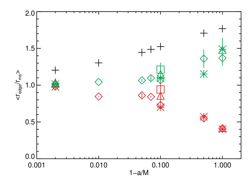
Figure 7: The location of the dissipation edge in relation to the location of the ISCO, $r_{ms}$, derived from $Q_{\mathrm{NT}}$ (black crosses), $Q_{\mathrm{AK}}$ (green symbols) and $Q_{\mathrm{MW}}$ (red symbols). The symbols correspond to different simulations as given in Figure 1.

4 Observed Quantities

Figure 8: The time-averaged fractional increase in luminosity, $\langle\Delta L_{\mathrm{AK}}\rangle$ derived from $Q_{\mathrm{AK}}$ for a distant observer located at $\theta_{o}=5^{\circ}$ (top left panel), $30^{\circ}$ (top centre panel), $45^{\circ}$ (top centre panel), $60^{\circ}$ (bottom left panel), $75^{\circ}$ (bottom centre panel) and $85^{\circ}$ (bottom right panel). Symbols correspond to different simulations as defined in Figure 1.

In the preceding sections, we have seen how stress near and inside the ISCO can significantly increase the total dissipation in the accretion flow and alter the location of the dissipation edge. In the NT model, all but $5\%$ of the total energy is dissipated outside of 1.2–1.8$r_{ms}$. By allowing for non-zero stress at the ISCO, the AK model moves the radial coordinate of the dissipation edge inward by factors of $\sim 0.8$ compared to the NT model. Relaxing the assumption that dissipation terminates at the ISCO causes the dissipation edge to move inside the ISCO. From an observational standpoint, these distinctions can be important. They affect the degree to which a given accretion flow can probe a black hole’s gravitational potential, and also determine such observables as the peak in the disc thermal spectrum and the width of the Fe K$\alpha$ line profile.

While the fluid frame dissipation is important, the real test is whether these differences carry over into the rest frame of a distant observer. In this section we examine this issue using the photon transfer function, which incorporates effects due to gravitational and orbital Doppler shifts, along with the influence of light-bending and gravitational lensing.

We will examine the properties of these discs in two ways: first, when observed from different inclination angles, and second by averaging over solid angle to obtain a total value. The solid angle averaged value of some observed quantity $m_{o}$ is defined as

$$\{M\}=\frac{\int{\int{m_{o}(\theta_{o})\sin\theta_{o}d\theta_{o}}d\phi}}{\int{\int{\sin\theta_{o}d\theta_{o}}d\phi}}.$$ (20)

The solid angle average of a given quantity is not itself observable, and for many potential observables the dependence on viewing angle is considerable. Nevertheless, the angle average provides a simple way to summarise the impact of the effects we are studying.

4.1 Fractional Increase in Luminosity

For a given dissipation model, we can compute the total luminosity carried to a distant observer using the observed flux, eqn.  3, and integrating:

$$\begin{split}L=\int\int g^{4}[x^{\mu}_{\mathrm{surf}}(\alpha,\beta)]Q[x^{\mu}_{\mathrm{surf}}(\alpha,\beta)]\times\\ \delta(E_{o}-gE_{e})d\alpha d\beta;\end{split}$$ (21)

$Q$ corresponds to $Q_{\mathrm{AK}}$, $Q_{\mathrm{NT}}$ or $Q_{\mathrm{MW}}$ as appropriate. We can then compute the fractional enhancement of the luminosity over the NT model using

$$\langle\Delta L_{\mathrm{AK,MW}}\rangle=\langle\frac{L_{\mathrm{AK,MW}}-L_{\mathrm{NT}}}{L_{\mathrm{NT}}}\rangle.$$ (22)

The results for the AK model are plotted in Figure 8 for a distant observer at inclinations ranging from 5–$85^{\circ}$. In §3.1 we found $\langle\Delta D_{\mathrm{AK}}\rangle$ was strongly correlated with black hole spin, ranging from 10–500% as $a/M$ approached one. Figure 8 shows that the corresponding fractional increases in luminosity are more modest, ranging between 5–$40\%$ for $\theta_{o}\leq 45^{\circ}$ (low inclinations) to substantially above $40\%$ for the half of solid angle with $\theta_{o}\geq 60^{\circ}$ (high inclinations). At low inclinations, $\langle\Delta L_{\mathrm{AK}}\rangle$ exhibits little dependence on black hole spin. At high inclinations, $\langle\Delta L_{\mathrm{AK}}\rangle$ exhibits a similar (if slightly weaker) dependence on black hole spin to that seen in $\langle\Delta D_{\mathrm{AK}}\rangle$.

Figure 9: As in Figure 8 for the time-averaged fractional increase in luminosity, $\langle\Delta L_{\mathrm{MW}}\rangle$ derived from $Q_{\mathrm{MW}}$.

Figure 9 gives $\langle\Delta L_{\mathrm{MW}}\rangle$ for the same range of inclinations. In §3.2 (see Fig. 4), we found $\langle\Delta D_{\mathrm{MW}}\rangle$ was generally within a factor of 2 of $100\%$, with little consistent dependence on black hole spin. Figure 9 shows a different picture. At all inclinations, $\langle\Delta L_{\mathrm{MW}}\rangle$ at the highest spin is a few tens of percent, varying by $\sim 2$ for the different magnetic topologies. At all inclinations, there is also a rise in $\langle\Delta L_{\mathrm{MW}}\rangle$ with diminishing spin, but the slope of this rise increases sharply with increasing inclination angle. As a result, for angles of $75^{\circ}$ and more, $\langle\Delta L_{\mathrm{MW}}\rangle\mathrel{\hbox{\hbox to0.0pt{\hbox{\lower 4.0pt\hbox{$\sim$}}\hss}\hbox{$>$}}}100\%$ for all spins $a/M\mathrel{\hbox{\hbox to0.0pt{\hbox{\lower 4.0pt\hbox{$\sim$}}\hss}\hbox{$<$}}}0.9$. There is a weak tendency for $a/M=0.5$ to yield the greatest fractional enhancement in luminosity, but it is not by a wide margin over the spinless case.

In §3.2 we found that the fraction of the total energy dissipated outside the ISCO ranged from $\mathrel{\hbox{\hbox to0.0pt{\hbox{\lower 4.0pt\hbox{$\sim$}}\hss}\hbox{$>$}}}60\%$ to $\mathrel{\hbox{\hbox to0.0pt{\hbox{\lower 4.0pt\hbox{$\sim$}}\hss}\hbox{$>$}}}80\%$ for non-dipolar magnetic field topologies. Figure 10 plots the fraction of the total luminosity that is received from outside of $r_{ms}$ for $Q_{\mathrm{MW}}$. This fraction is near $100\%$ for low inclinations and $a/M>0.9$. As the spin of the hole is reduced below $a/M=0.9$, the fraction falls to $\mathrel{\hbox{\hbox to0.0pt{\hbox{\lower 4.0pt\hbox{$\sim$}}\hss}\hbox{$>$}}}90\%$ as more photons escape from inside the ISCO. At higher inclinations ($\theta_{o}\geq 60^{\circ}$), the contribution from the plunging region increases for all but the most rapidly rotating black holes, in which $>80\%$ of the total observed luminosity originates outside of the ISCO. Thus, the contribution of the plunging region is greatest for low to moderate black hole spins: at high inclination the plunging region contributes 20–$60\%$ of the total observed luminosity of the disc for this range of spins.

The difference in solid angle averaged luminosity compared to the standard NT value is shown in Figure 11. Both $\{\Delta L_{\mathrm{AK}}\}$ and $\{\Delta L_{\mathrm{MW}}\}$ are 10–100%. $\{\Delta L_{\mathrm{AK}}\}$ generally increases with increasing $a/M$. There is considerable variation between simulations with different magnetic field topologies but with the same black hole spin. The AK model is sensitive to the precise value of the stress used at the ISCO, but even for the weakest stress values used here there are still significant increases in total luminosity.

In contrast, $\{\Delta L_{\mathrm{MW}}\}$ decreases with increasing $a/M$ and is largest for $a/M=0.5$ where $\{\Delta L_{\mathrm{MW}}\}\sim 100\%$ In fact, $\{\Delta L_{\mathrm{MW}}\}$ is larger than $\{\Delta L_{\mathrm{AK}}\}$ at low spin, but smaller at high spin, consistent with results obtained in the fluid frame. Two effects are important here. First, the plunging region is larger for low spin holes, so emission from that region (absent by assumption from the AK models) is more significant for those cases. Second, the stress tends to increase sharply at the ISCO for high spin holes, boosting the emission in the AK model. As we have already remarked in other contexts, different magnetic topologies produce significant variation among the simulations performed at a given black hole spin.

Figure 10: As in Figure 8 for the fraction of the total luminosity emitted outside of the ISCO derived from $Q_{\mathrm{MW}}$.

4.2 The Radiation Edge

The standard NT model is highly constrained. The assumption that stress goes to zero at the ISCO, the location of which is determined by the mass and spin of the hole, sets the location of the radiation edge. Removing this boundary condition means that the radiation edge can move, but by how much? As emphasised in the Introduction, one principal goal of this analysis is to locate the radiation edge for models that have nonzero stresses at the ISCO. While one might define the radiation edge as that point outside of which 100% of the light is emitted, such a definition fails to distinguish between the AK and NT models because for both this point is the ISCO. To bring out the distinctions in the distribution of the emission near the inner edge we define the radiation edge as the radius outside of which $95\%$ of the light that reaches distant observers is emitted. To further develop these contrasts, we also examine the cumulative distribution function for the fraction of the solid angle-averaged luminosity reaching infinity from outside a given radius.

In Figure 12 we plot the radiation edge for each of the dissipation models and for the same range of $\theta_{o}$ shown in Figures 8–10. The first thing to note is that the transport of photons to infinity introduces a significant separation between the radiation edge and the previously computed dissipation edge.

For the NT model at angles $\theta_{o}\leq 45^{\circ}$, the radiation edge lies between 1.7–$2.8r_{ms}$, increasing with increasing $a/M$, whilst for $\theta_{o}\geq 60^{\circ}$, the radiation edge becomes approximately independent of black hole spin and can be found between 1.3 and $1.7r_{ms}$. Comparing the location of the radiation edge to the dissipation edge reveals that, for $\theta_{o}\leq 45^{\circ}$, the radiation edge is either at (for spins $a/M<0.9$) or outside (for $a/M\geq 0.9$) the location of the dissipation edge. When the inclination is greater ($\theta_{o}\geq 60^{\circ}$), the radiation edge lies either inside ($a/M<0.9$) or near ($a/M\geq 0.9$) the location of the dissipation edge.

Similar behaviour is found for the AK radiation edge. The principal difference is that, in this case, the radiation edge lies inside that of the NT by a fraction that remains approximately constant as $\theta_{o}$ is varied, with variations only on the $\sim 5\%$ level for a given simulation. For example, for simulation KD0c, the AK radiation edge lies between $0.83-0.80$ of the NT radiation edge as $\theta_{o}$ varies between $5^{\circ}$ and $85^{\circ}$, whilst for simulation KDPg, this fraction ranges between $0.80-0.75$ over this same range of $\theta_{o}$. The larger the black hole spin, the greater the difference between the AK and the NT models. In other words, the relative visibility of the region near the ISCO remains the same function of spin and inclination angle for both models; the AK model simply has greater luminosity near the ISCO by an amount that increases with black hole spin.

We next consider the radiation edge derived from $Q_{\mathrm{MW}}$. In §3.3, we found that the location of its dissipation edge was inside that of the AK or NT model for all spins and field topologies. By contrast, the location of the radiation edge shows a wider range of behaviours. At any given inclination, the radiation edge moves to larger $r/r_{ms}$ as the spin increases. For a given spin, the radiation edge moves inward as the inclination grows. Specifically, for discs that are viewed almost face-on ($\theta_{o}=5^{\circ}$), the radiation edge lies between 1–$3r_{ms}$, increasing with increasing black hole spin. At this inclination, the radiation edge lies approximately a factor of three outside the location of the dissipation edge, independent of black hole spin. At moderate inclinations ($30^{\circ}\leq\theta_{o}\leq 45^{\circ}$), the radiation edge moves inwards towards the ISCO, ranging between 0.5 and $2.5r_{ms}$, and again increasing with increasing black hole spin. For $\theta_{o}<45^{\circ}$ and $a/M>0.9$, the radiation edge lies either at or outside that derived from $Q_{\mathrm{NT}}$ and $Q_{\mathrm{AK}}$, whilst for $a/M<0.9$ the radiation edge lies either at or inside that derived from $Q_{\mathrm{NT}}$ and $Q_{\mathrm{AK}}$.

Figure 11: Solid angle averaged $\{\Delta L_{\mathrm{AK}}\}$ (left panel) and $\{\Delta L_{\mathrm{MW}}\}$ (right panel). Symbols are as described in Fig. 1.

These trends in the location of the radiation edge, and in particular, the way it is offset from the dissipation edge (§3.3) are driven by the way photons travel through the relativistic potential. When the disc is viewed face-on, gravitational redshift dominates, reducing both the energy of photons emitted close to the hole and the apparent rate at which they are released; consequently, the radiation edge tends to move outward as the inclination angle becomes smaller. As the viewing direction moves closer to edge-on, Doppler boosting of the approaching side of the disc increases the energy of photons radiated there and their rate of emission, bringing the radiation edge inward. In the NT and AK models, all velocities are azimuthal, so the peak approach velocity occurs for matter passing through the sky plane when our view is nearly in the disc equatorial plane; however, in the MW model, the inward radial speed can be great enough, especially in the plunging region, for Doppler boosting also to enhance the luminosity of matter on the far side of the black hole. In all models, emission from the far side of the hole is also strengthened by gravitational lensing when the line of sight is near the disc plane. Thus, the radiation edge moves inward as the observer approaches the disc plane.

Trends in the position of the radiation edge as a function of black hole spin at fixed inclination angle are the result of a different trade-off. As the spin increases, the ISCO moves inward and all relativistic effects are strengthened. Those described in the previous paragraph tend, on balance, to make the radiation brighter as the inclination angle grows. However, as the spin increases, the fraction of all photons captured by the black hole also increases, likewise because the ISCO moves inward. In terms of how far inside the ISCO the radiation edge falls, the latter effect is the strongest: the ratio of the radial coordinate of the radiation edge to $r_{ms}$ is least for low-spin black holes viewed nearly edge-on.

One surprising result demands special discussion: at the highest spin ($a/M=0.998$) and small inclination angle ($\theta_{o}\leq 30^{\circ}$), the MW radiation edge either coincides with or lies a little bit outside the NT edge, and both the MW and NT edges are well outside the AK edge. At such high spin, photons escaping to infinity in the polar direction are severely redshifted if their point of origin is near or inside the ISCO. For this reason, all three radiation edges in this regime are at radii several times $r_{ms}$. As we have already discussed, however, when the spin is this rapid, the AK model predicts a rather larger dissipation rate in this range of radii than is predicted by either MW or NT. The disparity between the AK radiation edge on the one hand and the MW and NT edges on the other follows directly from this contrast. In addition, the radiation edge for one high-spin simulation (KDEa) appears to fall at particularly large radius, although this may well be an artefact of the lack of inflow equilibrium in this particular simulation (Krolik et al., 2005)

The radiation edge associated with the solid angle-averaged luminosity is shown in Figure 13. For $Q_{\mathrm{NT}}$, it lies between 1.5–1.8$r_{ms}$ and slowly increases with increasing black hole spin. For all models as the spin increases, photons radiated deeper in the potential are subject to larger gravitational redshifts and are more likely to be captured. For $Q_{\mathrm{AK}}$, the radiation edge moves inwards to 1.3–1.6$r_{ms}$, with the smallest values occurring for $a/M=0.9$ and increasing as one moves away from this spin in either direction. For this model the enhanced dissipation at the ISCO compensates somewhat for the greater likelihood for photon capture with increased black hole spin. For $Q_{\mathrm{MW}}$, the radiation edge lies between 0.5–1.7$r_{ms}$, increasing with increasing black hole spin. The enhanced dissipation within the plunging region boosts the luminosity (and reduces the radius of the radiation edge) for low spin models, but has little effect for high spins.

Regardless of spin the solid angle-averaged radiation edge derived from the simulation data lies within that of the NT model; enhanced stress always moves this point inward. Comparing $Q_{\mathrm{AK}}$ and $Q_{\mathrm{MW}}$ we find a more complex picture. The radiation edge in the AK model must, by assumption, lie outside the ISCO, but for the models with stress in the plunging region this need not be the case. Indeed, for low spin holes the radiation edge can be inside the ISCO, but the dissipation in the plunging region becomes less important as black hole spin increases. What matters most is the dissipation level outside of the ISCO. For the cases considered here, the stress rises rapidly at the ISCO for high-spin models and the semi-analytic AK formula predicts greater dissipation outside the ISCO than is implied by the stress levels seen in the simulations. Hence, for $a/M>0.9$ the solid angle-averaged radiation edge derived from $Q_{\mathrm{MW}}$ lies outside that derived from $Q_{\mathrm{AK}}$. This clearly illustrates that the location of the radiation edge can be very sensitive to the dissipation levels near the ISCO.

We have defined the radiation edge as the the radius outside of which $95\%$ of the total observed luminosity is emitted. This choice was made to provide a simple measure by which to contrast the different luminosity profiles associated with each of the dissipation models. In Figure 14 we plot the solid-angle averaged fractional cumulative distribution of observed luminosity, $\{F(r/r_{ms})\}$ for each of the dissipation models and individual datasets. We see that for $0.2\leq F\leq 0.95$, all these curves may be fitted to a reasonable degree of approximation by the form $\{F(r/r_{ms}\})\propto\exp[-(r/r_{ms})/r_{*}]$. Thus, there is a characteristic radial scale for the luminosity profile that is always related to, but not necessarily identical to, $r_{ms}$, and it may be adequately parameterized by choosing a fiducial level of $F$.

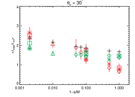
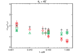
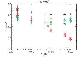
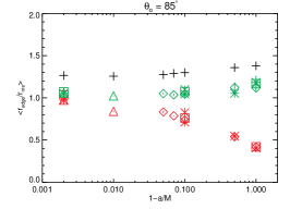
Figure 12: Time-averaged “radiation edge” seen by distant observers in in six different directions (arranged as in Fig. 8: $\theta_{o}=5^{\circ}$ (top left panel), $30^{\circ}$ (top centre panel), $45^{\circ}$ (top centre panel), $60^{\circ}$ (bottom left panel), $75^{\circ}$ (bottom centre panel) and $85^{\circ}$ (bottom right panel). The different models are coded by differently coloured symbols: $Q_{\mathrm{NT}}$ (black), $Q_{\mathrm{AK}}$ (green) and $Q_{\mathrm{MW}}$ (red). Different symbol shapes denote different simulations, as for Figure 1: The dipolar field simulations described by De Villiers et al. (2003) are shown by stars, those described by Hawley & Krolik (2006) by diamonds and the new high spin cases computed for this paper by triangles. Simulations with quadrupolar topologies are shown by squares. The toroidal field simulation ($a/M=0.9$) is denoted by a cross.

The plots also provide a quantitative sense of the potential importance of nonzero stress at the ISCO. First, note that the luminosity profile in the NT model is practically independent of spin (as can also be inferred from the solid-angle averaged radiation edge shown in Figure 13). This somewhat surprising result can be understood in terms of the dependence of the radiation edge on $\theta_{o}$. At small inclination angle (face-on views), the radiation edge derived from the NT model for slowly spinning black holes lies inside that of the rapidly spinning holes (relative to the location of the ISCO), whilst at large inclination angles the reverse is true. When this data is averaged over solid angle, these changes cancel and so the position of the radiation edge (and hence the fractional luminosity distribution) relative to $r_{ms}$ is independent of $a/M$. The NT model is so tightly constrained by its assumptions that when the dependencies due to observing angle are removed, there remains almost no contrast other the location of the ISCO which is set by the spin of the hole.

4.3 Characteristic Temperature

We have seen how the apparent size of the disc varies with spin, inclination and dissipation model. However, observations do not directly measure the radiation edge. Rather, the concept of a radiation edge is incorporated into the interpretation of the $L=A(a/M,\theta)T^{4}$ relationship Gierliński & Done (2004). We have already seen how changes in the dissipation function due to non-zero stress at and inside the ISCO have the potential to change the apparent area and luminosity of the disc. In this section, we attempt to gauge the impact of these changes on the characteristic temperature of the accretion flow, $T_{char}$, as it might be inferred from continuum fitting to the soft component of a spectrum. Our analysis must necessarily be simple. We define $T_{char}$ as the maximum (observed) blackbody temperature found anywhere in the disc. It is determined by defining an effective temperature in the fluid frame: $T_{eff}(r)=[Q(r)/\sigma]^{1/4}$ and then transforming this temperature to the rest frame of a distant observer via $T_{o}(r)=gT_{eff}(r)$ Cunningham (1975). Then, since the characteristic temperature of the associated blackbody spectrum will be very close (but not identical to) the maximum black body temperature, we make the approximation $T_{char}\sim\mathrm{max}(T_{o})$. We perform the same procedure for all three dissipation models, ignoring color temperature corrections and all observational effects except those due to inclination angle.

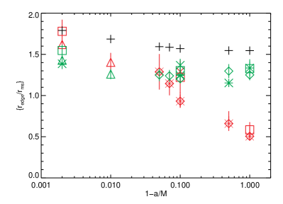
Figure 13: Solid angle averaged $\{r_{edge}/r_{ms}\}$. Symbols are as in Figure 7

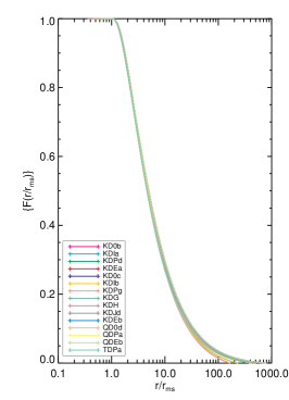
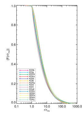
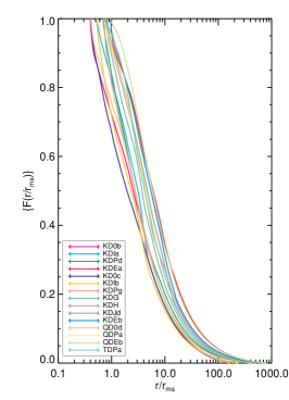
Figure 14: Solid-angle averaged fractional distribution of observed luminosity, $\{F(r/r_{ms})\}$ derived from $Q_{\mathrm{NT}}$ (left-hand panel), $Q_{\mathrm{AK}}$ (centre panel) and $Q_{\mathrm{MW}}$ (right-hand panel).

Although the geometric size of the disc in the AK model is the same as in the NT model (the curves are still constrained to reach $100\%$ at the ISCO), the middle panel of Figure 14 shows how the addition of a finite amount of stress at the ISCO breaks the NT degeneracy. The most significant differences come, naturally, from including contributions from inside the ISCO. The curves for the $Q_{MW}$ models (right hand panel) are well separated for different spins. For these models, the relative importance of the plunging region is a function of both the amplitude of the stress there and the spin of the hole. The farther the ISCO from the horizon, the greater the chance for radiation within the plunging region to escape.

$T_{char}$ is plotted in Figure 15 for the different dissipation functions and observer inclinations shown in Figure 12. Each of the accretion flows has been scaled such that its accretion rate would produce a flow with luminosity $0.1L_{edd}$. Several features are immediately apparent. At all inclinations $T^{NT}_{char}$, the characteristic temperature associated with $Q_{NT}$ increases with increasing $a/M$. This well known result is the foundation of attempts to measure black hole spin with spectral fitting techniques. $T^{AK}_{char}$ shows a similar trend, with an increase over $T^{NT}_{char}$ by a factor $1.1-1.4$, an amount that is comparable to typical color corrections (see e.g. Done & Davis, 2008). The AK model has the same (fixed) inner boundary, but has enhanced luminosity for the same accretion rate. The effect is most significant for large inclination angles.

$T^{MW}_{char}$ exhibits a different behaviour. At low spins, $T^{MW}_{char}$ is significantly greater than $T^{NT}_{char}$, whilst at high spins the contrast is reduced. Overall, this has the effect of making $T^{MW}_{char}(a/M)$ almost constant for a given inclination. Overall, $T^{MW}_{char}/T^{NT}_{char}$ varies between a factor of $1.8-2.3$ for accretion flows accreting at the same luminosity, with the greatest increases occurring for slowly spinning black holes viewed nearly edge on. Because energy extraction and radiation occur within the plunging region, the distinctions between holes with different spins is greatly reduced. In other words, the effective inner boundary for all discs lies close to the horizon.

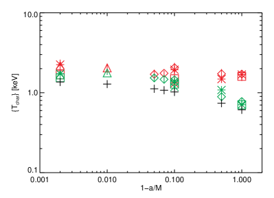
Figure 16: Plot showing solid angle averaged $\{T_{char}\}$ . Symbols are as in Figure 7

These effects are summarised in Figure 16, where we plot the characteristic temperature associated with the solid-angle averaged radiation edge for a black hole accreting at $0.1L_{edd}$. Both the NT and the AK model share the ISCO as their inner boundary, and as a result both $T^{NT}_{char}$ and $T^{AK}_{char}$ increase by around a factor of two over the range of $a/M$ shown here (both increasing with increasing $a/M$). On the other hand $T^{MW}_{char}$ is approximately constant over the same range of spin and is greater than $T^{NT}_{char}$ by a factor that falls from $\simeq 2.3$ to $\simeq 1.2$ as $a/M$ increases from 0 to 0.998. Unlike the radiation edge, the contrast between $T^{MW}_{char}$ and both $T^{AK}_{char}$ and $T^{NT}_{char}$ always has the same sense: the MW model always predicts a higher characteristic temperature.

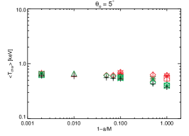
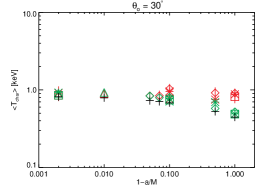
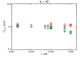
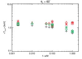
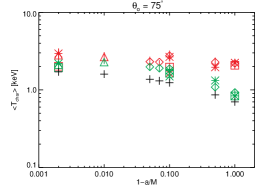
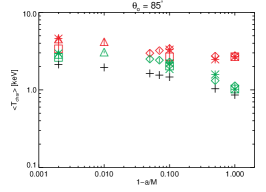
Figure 15: Time-averaged characteristic black body temperature for a $10M_{\odot}$ black hole accreting at $0.1L_{edd}$ measured by distant observers in in six different directions (arranged as in Fig. 12, with the same key as that figure).

4.4 Impact on Measurements of $a/M$

In the previous section, we examined the consequences of stress at the ISCO on the characteristic temperature of the accretion flow and the dependence of this quantity on both black hole spin and inclination. We now examine this question from the opposite direction, i.e., supposing one has a measurement of the characteristic temperature of an accretion disc in a particular system (along with the black hole mass, inclination of the binary orbit and disc luminosity), how much uncertainty in the determination of $a/M$ is induced by uncertainty about the correct dissipation profile in the inner disc?

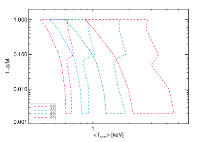
Figure 17: Plot showing the region of the $(T_{char},a/M)$-plane consistent with a given value of $\theta_{o}$ for a $10M_{\odot}$ black hole accreting at $0.1L_{edd}$. Different colors correspond to different $\theta_{o}$ (see key in bottom left corner of plot), dot-dash lines show the $T_{char}$ curve predicted by $Q_{NT}$ at a given $\theta_{o}$, and the region enclosed by the dot-dash and dashed lines of a given color show the region of the $(T_{char},a/M)$-plane consistent with that value of $\theta_{o}$.

To address this question, we use the data shown in Figure 15 to construct Figure 17, in which four polygons, one for each of four different inclinations, illustrates the range of $T_{char}$ and $a/M$ consistent with the different disc models. To produce this figure, we first fixed the inclination, spin, and black hole mass, and then collected the values of $T_{char}$ predicted on the basis of any of our three candidate models (NT, AK, and MW) from any of the several simulations we conducted with that particular spin parameter. The left-hand edge of each region traces the prediction of the NT model because it always gives the lowest temperature. The horizontal width of each region is defined by the range of temperatures predicted by the complete complement of models and simulations. Because we have conducted simulations at seven different spins, the right-hand edge is defined at seven points.

Several qualitative features emerge from study of this figure. First, for each inclination, the maximum temperature change predicted by the NT model as the spin runs from $a/M=0$ to $a/M=0.998$ (generally about a factor of 2) is always less than the maximum temperature change at zero spin due to model-dependent uncertainty in the dissipation profile (typically a factor of 3). Thus, if we knew the inclination angle and mass for a given black hole, but not its spin paramater, our uncertainty in predicting $T_{char}$ has a greater contribution from our uncertainty about disc physics than it does from our ignorance of its value of $a/M$.

Second, suppose that we know the inclination angle of a particular black hole and obtain $T_{char}$ from X-ray spectra. The uncertainty in $a/M$ due to uncertainty in the dissipation profile may be estimated by imagining a vertical line at that value of $T_{char}$ running through the region for the appropriate inclination angle. The uncertainty is then given by the difference in spins between the points where the line intersects the boundary of the region. The size of this uncertainty tends to be larger when our view is more nearly edge-on. However, for almost any value of $T_{char}$ that is consistent with any of the area of a region, the magnitude of the uncertainty in $1-a/M$ is generally at least an order of magnitude.

Still another way to look at this diagram is to ask, “If we estimate spin by using the NT model, by how much may it be wrong if a different model is truer to the disc’s radiation profile?” The answer is the span of a vertical line whose lowest point is the NT prediction and runs to the upper boundary of the associated region. Because the NT model always gives the lowest prediction for $T_{char}$, the spin inferred from it is always the greatest possible spin, and the error bar always stretches toward lower rotation rates. Given the characteristic curvature of the permitted regions in this plane, the magnitude of the possible error in $1-a/M$ tends to be larger (in logarithmic terms) when the NT inference of $a/M$ is closer to unity, but can still be substantial even when $a/M\mathrel{\hbox{\hbox to0.0pt{\hbox{\lower 4.0pt\hbox{$\sim$}}\hss}\hbox{$<$}}}0.9$. Note, however, that we only present data for $a/M>0$, so we cannot provide an explicit lower bound on the range of $a/M$, beyond stating that $a/M=0$ in the magnetized case is always consistent with the full range of $a/M$ in the NT case for fixed $\theta_{o}$.

5 Summary, Discussion and Conclusions

That magnetic forces might cause substantial stress at the ISCO was foreseen very shortly after the invention of the standard model Page & Thorne (1974). This possibility now appears to be an immediate corollary of the well-established result that MHD stresses account for most of the angular momentum transport in the bodies of accretion discs. Indeed, such stresses were seen in the first generation of three dimensional GRMHD disc simulations. The goal of this paper has been to begin the linkage of these numerical MHD simulations to the observable properties of accreting black holes even before the simulations are fully equipped to make predictions about how these systems radiate. To do so, we have followed a path of cautious extrapolation from older methods. We first used simulation data to fix the single parameter of a model (called AK here) that changes the previous standard (the Novikov-Thorne model) only by admitting the possibility of a non-zero stress at the ISCO. Because the AK model is defined in a way that prevents its extrapolation within the ISCO, we used the formalism underlying both it and the NT model (i.e., vertically-integrating and azimuthally- and time-averaging the equation of momentum-energy conservation under the assumption that the four-velocity and the stress tensor are orthogonal) to create an expression for the dissipation (called $Q_{\mathrm{MW}}$ here) valid both inside and outside the ISCO.

Happily, in the body of the accretion disc well outside the ISCO, both the AK and the MW method agree fairly well with NT more or less independent of black hole spin and magnetic field topology, although the irregularity in the curves of Figure 2 reminds one that the simulations are dynamic and time-varying, and that the 26 samples of simulation data we used define only somewhat imperfectly the long-term time-average. In addition, with the exception of the extreme high-spin example, where the AK and MW methods depart from NT just outside the ISCO, they do so together. This is noteworthy because, although they are based on closely-related formalisms, they are not identical: perhaps their most significant contrast is that the AK method assumes that $u_{r}=0$, while the MW method does not. Lastly, inside the ISCO, where only the MW method is defined, it follows a smooth extrapolation from larger radius. When the black hole spins slowly ($a/M\mathrel{\hbox{\hbox to0.0pt{\hbox{\lower 4.0pt\hbox{$\sim$}}\hss}\hbox{$<$}}}0.9$), $Q_{\mathrm{M}W}$ extends with hardly any change in logarithmic derivative with respect to radius. For higher spin, the extension gradually steepens toward smaller radius, but the next step in our formalism shows that this makes little difference to observed radiation: relativistic ray-tracing shows that the volume deep inside the plunging region, particularly at high spin, contributes little energy to the luminosity reaching observers at infinity. Thus, we are relatively confident that, despite the uncertainties involved, our estimate of the location of the radiation edge is comparatively insensitive to the exact relation between the flow’s detailed dynamical properties and the dissipation rate.

The dependence of the radiation edge on spin may be summarised succinctly: At the highest spin, there is relatively little difference between the different methods of estimating its position because the ISCO is so close to the horizon that the great majority of photons released in the plunging region never reach infinity, or if they do, are severely redshifted. It moves from 2–3 times the radius of the ISCO when the disc is viewed face-on to almost exactly at the ISCO when the disc is viewed nearly edge-on. This inward movement of the radiation edge with increasing inclination angle is quite model-independent, as it stems from relativistic photon propagation effects: when photons from the plunging region do reach infinity with substantial energy, it is because they are emitted in the direction of the orbital motion. Probability of escape is then enhanced by a combination of special relativistic beaming and gravitational lensing; energy at infinity is enhanced by special relativistic Doppler boosting. As the black hole spin decreases, the diminishing depth of the potential immediately inside the ISCO makes it progressively easier for photons to escape from that region and reduces the gravitational redshift they suffer when they do. The result is that the radiation edge moves farther inside the ISCO as either the spin diminishes (at fixed viewing angle) or the inclination angle moves toward the equatorial plane (at fixed spin). At its most extreme, the case of $a/M=0$ and $\theta_{o}=85^{\circ}$, $r_{re}$ can be $\simeq 0.5r_{ms}$.

Figure 10 gives additional cause to believe that these results are comparatively insensitive to dissipation model. Although the radiation edge can move well inside the ISCO at low spin and high inclination, most of the light received by distant observers is generally emitted in the region near and outside the ISCO. Only at the highest inclinations ($\theta_{o}\mathrel{\hbox{\hbox to0.0pt{\hbox{\lower 4.0pt\hbox{$\sim$}}\hss}\hbox{$>$}}}75^{\circ}$) and lowest spins ($a/M\mathrel{\hbox{\hbox to0.0pt{\hbox{\lower 4.0pt\hbox{$\sim$}}\hss}\hbox{$<$}}}0.5$) does the contribution of the plunging region to the luminosity approach $50\%$. Thus, most of the light seen at infinity likely comes from a region where the predictions of the AK and the MW models differ little.

Nonetheless, because it is also true that most of the light is emitted within a radius at most a few times the ISCO (except for the highest spin viewed more or less face-on), the contrast in total luminosity between the AK and MW models on the one hand, and the NT on the other, are order unity for all spins $\leq 0.9$. For higher spins, the effect may be smaller, but the uncertainties are also greater.

These conclusions have immediate implications for a number of phenomenological issues. Firstly, as suggested by Falcke et al. (2000), it may be possible to image the nearest supermassive black hole, the one in Sgr A*. Because its accretion flow, unlike those of intrinsically brighter systems, could well be radiatively inefficient, a simulation scheme that conserves total energy is more appropriate to analysing its emission. Noble et al. (2007), using such a code (albeit an axisymmetric version), have produced predicted images that illustrate several of the effects emphasised here, although in their work so far they have not reported quantitative descriptions of characteristic emission radii.

Secondly, the enhanced total radiative efficiency due to dissipation in the marginally stable region may affect estimates of population-mean spin parameters (e.g., as for AGN by Elvis et al., 2002; Yu & Tremaine, 2002). Because the efficiency rises with increasing prograde spin in the NT model, the spin inferred by this method may overestimate the actual spin of accreting black holes if this enhancement is ignored.

The additional luminosity from enhanced stress in the innermost part of the accretion flow could significantly alter the emergent spectrum. Employing a simple thermal model, we have found that the characteristic temperature of the flow increases by a factor of 1.2 –1.4 over that predicted by the NT model. As a consequence, the thermal peak of the disk spectrum (at $\sim 1$ keV in Galactic black holes, $\sim 10$ eV in AGN) may be pushed to somewhat higher energies.

Several caveats must be mentioned, however, in regard to this prediction. First, this number supposes an emergent spectrum that is Planckian, but most estimates of the disc atmosphere’s structure suggest that it is scattering-dominated, so that the color temperature of the spectrum is shifted upward from the effective temperature. The magnitude of this shift depends on details of the disc’s vertical structure that are not as yet well known (see e.g. Davis et al., 2005). Furthermore, Blaes et al. (2006) (using the vertically stratified shearing box simulations of Hirose et al., 2006) show that magnetic pressure support changes the vertical structure of the disk resulting in a noticeable hardening of the emergent disk spectrum compared to the standard Novikov-Thorne picture due to non-LTE effects. Second, it is possible that some of the enhanced dissipation will occur where the density and optical depth are too low to accomplish thermalisation. Strengthening of the “coronal”, i.e., hard X-ray, emission, rather than hardening the thermal disc spectrum would then be the likely consequence. Third, our treatment ignores those photons emitted deep in the potential that neither escape directly to infinity nor are captured by the black hole, but instead strike the disc. As shown by Agol & Krolik (2000), this “returning radiation” can be a substantial fraction of all photons emitted when $r\mathrel{\hbox{\hbox to0.0pt{\hbox{\lower 4.0pt\hbox{$\sim$}}\hss}\hbox{$<$}}}5r_{g}$. Depending on their spectrum and the structure of the disc atmosphere where they strike, these photons may be either reflected (with Doppler shifts) or absorbed and their energy reradiated at a different (in general, lower) temperature. Quantitatively evaluating all three of these effects is well beyond the scope of this paper, but can be done in future work.

There are also implications for attempts to determine black hole spin from spectral fitting. In all three models, the characteristic radius of emission is always near the ISCO, but does not, in general, coincide with it. Generally speaking, this characteristic radius is largest for the NT model, smaller (but still outside the ISCO) for the AK model, and smaller still, possibly moving into the plunging region inside the ISCO, for the MW model. Because the ISCO moves to smaller radial coordinate as $a/M$ increases, these characteristic radii always become smaller for faster spin. However, the fractional amount by which the characteristic emission radius moves inward in the MW model is greatest for the lowest spins, so that in the end, the MW model predicts a relatively slow variation of radiation edge with black hole spin. The AK model, like the NT model, does not radiate from inside the ISCO, but the additional stress at and just outside the ISCO in this model (relative to the NT prediction) produces a systematic increase in the characteristic temperature. The magnitude of this shift in characteristic temperature rises, of course, with increasing additional stress. When there is emission from the plunging region, as in the MW model, the characteristic temperature can rise still higher, but the highly relativistic motions there make observed properties more strongly dependent on inclination angle. In addition, a larger fraction of the emitted photons can be captured by the black hole.

When all these considerations are combined, we find that, for fixed black hole mass, luminosity, and inclination angle, the uncertainty in the characteristic temperature of the radiation reaching distant observers due to uncertainty in the dissipation profile is greater than the that due to a complete lack of knowledge of the black hole’s spin. Clearly, our incomplete understanding of accretion disc physics (here specifically the magnitude of the stress at and inside the ISCO) makes it difficult to determine a black hole spin based on continuum model-fitting. The best one can say is that estimates based on the traditional Novikov-Thorne model can be expected to yield the most rapid spin possible, but the actual spin may be significantly slower.

Our results demonstrate the potential importance of nonzero stresses at and inside the ISCO. But how representative are the specific values obtained in these simulated discs? There are two considerations: those arising from purely numerical effects, and those limitations arising from the assumptions and parameters of the model used.

First, the results of numerical simulations can be influenced by finite resolution and the limitations of the numerical technique. All of the simulations presented in this work were performed at a resolution of $192\times 192\times 64$ $(r,\theta,\phi)$ grid zones using ideal MHD and an internal energy equation. The equation of state and the numerical energy dissipation are unlikely to have a direct effect on our conclusions as $Q_{MW}$ is derived directly from the physical Maxwell stresses within the disc, rather than by measuring some numerical dissipation rate. Low resolution usually causes the Maxwell stress to be undervalued; if so, the implications of this paper would be strengthed by improved resolution. Until available computer power makes better-resolved three-dimensional simulations possible, the best way we have to test the effects of finite resolution is to compute axisymmetric simulations with higher resolution. A variety of such simulations were presented in Beckwith et al. (2008) with resolutions up to $1024^{2}$. We observe that greater resolution reduces the rate of numerical reconnection and improves the ability of the simulation to maintain certain field configurations and small-scale field structures. Overall the amplitude of the turbulent Maxwell stresses in the disc remained largely unchanged as resolution was increased. We have also calculated ${\cal W}^{(r)}_{(\phi)}$ and $Q_{MW}$, and find no significant qualitative differences from the results presented in this work.

Beyond the purely numerical issues, the value of the Maxwell stress at the ISCO may depend on a number of disc properties. In the ensemble of simulations presented here, the stress levels are determined in part by the initial field topology (dipole versus quadrupolar, poloidal versus toroidal, and the presence or absence of a net vertical field). Indeed, local shearing-box simulations suggest that the saturated field strength can increase substantially when large-scale vertical field threads the disc Balbus & Hawley (1998).

It is also possible that the saturation stress depends on disc thickness. To quantify disc thickness, we define the scale-height $H$ as the proper height above the plane at which the time- and azimuthally-averaged density falls by $1/e$ from its similarly averaged value on the equatorial plane (see §3): $H=\int^{\theta_{h}}_{\pi/2}\sqrt{g_{\theta\theta}(r=3M,\theta)}d\theta$. We similarly define $R$ as the proper (as opposed to coordinate) radial distance from the horizon to $3M$ plus the coordinate distance from the origin to the horizon: $R=r_{in}+\int^{r=3M}_{r_{in}}\sqrt{g_{rr}(r,\theta=\pi/2)}dr$, with $r_{in}$ as given in Table 1). We then define the disc thickness as the ratio $H/R$. Even though $r=3M$ lies well within the plunging region for the lower spin cases, we find that there is a slow enough radial variation in this quantity to make $H/R$ a reasonably well-defined parameter. Measured in this way, our discs are modestly thick, with a characteristic aspect ratio $H/R=0.06$–0.2 at $r=3M$. Most of the range in $H/R$ results from the fact that the maximum pressure in the initial condition for these simulations varies somewhat between different $a/M$.

It is difficult to say, however, just what sort of dependence there may be on disc thickness. There are some arguments suggesting that magnetic effects may increase with increasing $H/R$. For example, local shearing-box simulations find that the Maxwell stress is proportional to magnetic pressure Balbus & Hawley (1998); Sano et al. (2004), but there have not yet been any systematic studies of what regulates the magnetic pressure in global, vertically-stratified discs. Afshordi & Paczyński (2003) have argued that inner disc stresses and dissipation may depend on disc thickness as well as on accretion rate, an argument reiterated by Shafee et al. (2007), but their arguments are framed in an essentially hydrodynamic context, and therefore eliminate any possibility of predicting magnetic stresses. They are also non-relativistic, and therefore eliminate any effects due to frame-dragging. There are also arguments that any dependence on $H/R$ may be weak. In the simplest analytic or quasi-analytic MHD models, magnetic torques at the ISCO remain significant even in the limit of a zero pressure disc (Krolik, 1999; Gammie, 1999). As discussed in Krolik et al. (2005), processes analogous to the Blandford-Znajek mechanism can readily transport energy and angular momentum from rotating black holes to the accretion flow, and there is no particular reason to think that these processes should be tightly connected to the pressure in the disc. In the end, only direct simulations with the resolution to describe thin discs adequately will answer this question in a satisfactory way. The results of the present investigation provide yet one more reason why it will be important to do so.

The final question that we address in this work is how the results presented here relate to current state of the art measurements of black hole spin via spectral fitting of the disk continuum. The 6 systems with the best data (see e.g. Davis et al., 2006; Shafee et al., 2006; Middleton et al., 2006; Liu et al., 2008) all have spins in the range $a/M\sim 0.1-0.8$ based on disk models that assume the stress-free inner boundary condition. From the perspective of the disk stress models these spins are upper limits. This might indicate that the hole is counter-rotating, but also opens the possibility that spin determinations might themselves constrain the physics near the ISCO. Firstly, the stress levels at the ISCO could be near the value assumed by the stress-free inner boundary condition; secondly, the classical relationship between stress and dissipation might not hold for enhanced magnetic stresses ear the ISCO; thirdly, the density levels at and inside the ISCO could be insufficient to thermalize the dissipated heat; fourthly, the time-scales for thermalization and radiation of the dissipated heat could be longer than the inflow time-scale. Another uncertainty which we have not examined is that the plane of the disk and the equatorial plane of the hole could be misaligned and so the disk is subject to the Bardeen-Peterson effect (see e.g. Fragile et al., 2007). Understanding the roles played by the these effects will be crucial in providing robust estimates of black hole spins via spectral fitting of the disk continuum.

Appendix A Basis Vectors of the Local Rest Frame

The calculation of the photon transfer functions requires the introduction of a set of basis vectors describing the local rest frame of the fluid (the “fluid frame”). Such a tetrad set was presented by Krolik et al. (2005), who used a Gram-Schmidt orthonormalization procedure to construct it. Unfortunately, some of the expressions given in that work were incorrectly transcribed. The correct version is as follows:

$$e^{\mu}_{(t)}=u^{\mu}$$

$$e^{\mu}_{(\phi)}=-\frac{1}{k_{\phi}\sqrt{|-g^{2}_{t\phi}+g_{\phi\phi}g_{tt}}|}\times$$

$$\left[g_{\phi\phi}u^{\phi}+g_{t\phi}u^{t},0,0,-\left(g_{t\phi}u^{\phi}+g_{tt}u^{t}\right)\right]$$

$$e^{\mu}_{(r)}=-\frac{1}{k_{r}k_{\phi}}\left[\sqrt{g_{rr}}u^{r}u^{t},\frac{k^{2}_{\phi}}{\sqrt{g_{rr}}},0,\sqrt{g_{rr}}u^{r}u^{\phi}\right]$$

$$e^{\mu}_{(\theta)}=-\frac{1}{k_{\theta}k_{r}}\left[\sqrt{g_{\theta\theta}}u^{\theta}u^{t},\sqrt{g_{\theta\theta}}u^{\theta}u^{r},\frac{k^{2}_{r}}{\sqrt{g_{\theta\theta}}},\sqrt{g_{\theta\theta}}u^{\theta}u^{\phi}\right]$$

where:

$$k_{\phi}=\sqrt{|g_{\phi\phi}\left(u^{\phi}\right)^{2}+u^{t}\left(2g_{t\phi}u^{\phi}+g_{tt}u^{t}\right)|}$$

$$k_{r}=\sqrt{|g_{\phi\phi}\left(u^{\phi}\right)^{2}+g_{rr}\left(u^{r}\right)^{2}+u^{t}\left(2g_{t\phi}u^{\phi}+g_{tt}u^{t}\right)|}$$

$$k_{\theta}=\sqrt{|g_{\phi\phi}\left(u^{\phi}\right)^{2}+g_{rr}\left(u^{r}\right)^{2}+g_{\theta\theta}\left(u^{\theta}\right)^{2}+u^{t}\left(2g_{t\phi}u^{\phi}+g_{tt}u^{t}\right)|}$$

References

- Afshordi & Paczyński (2003) Afshordi N., Paczyński B., 2003, ApJ, 592, 354
- Agol & Krolik (2000) Agol E., Krolik J. H., 2000, ApJ, 528, 161
- Armitage & Reynolds (2003) Armitage P. J., Reynolds C. S., 2003, MNRAS, 341, 1041
- Balbus et al. (1994) Balbus S. A., Gammie C. F., Hawley J. F., 1994, MNRAS, 271, 197
- Balbus & Hawley (1998) Balbus S. A., Hawley J. F., 1998, Reviews of Modern Physics, 70, 1
- Balbus & Papaloizou (1999) Balbus S. A., Papaloizou J. C. B., 1999, ApJ, 521, 650
- Bardeen et al. (1972) Bardeen J. M., Press W. H., Teukolsky S. A., 1972, ApJ, 178, 347
- Beckwith & Done (2004) Beckwith K., Done C., 2004, MNRAS, 352, 353
- Beckwith & Done (2005) Beckwith K., Done C., 2005, MNRAS, 359, 1217
- Beckwith et al. (2008) Beckwith K., Hawley J. F., Krolik J. H., 2008, ApJ, 678, 1180
- Blaes et al. (2006) Blaes O. M., Davis S. W., Hirose S., Krolik J. H., Stone J. M., 2006, ApJ, 645, 1402
- Brankin & Shampine (1991) Brankin R. W., Shampine L. F., 1991, Technical report, RKSUITE: A suite of Runge-Kutta codes for the initial value problems for ODEs. Souther Methodist University
- Brenneman & Reynolds (2006) Brenneman L. W., Reynolds C. S., 2006, ApJ, 652, 1028
- Cunningham (1975) Cunningham C. T., 1975, ApJ, 202, 788
- Davis et al. (2005) Davis S. W., Blaes O. M., Hubeny I., Turner N. J., 2005, ApJ, 621, 372
- Davis et al. (2006) Davis S. W., Done C., Blaes O. M., 2006, ApJ, 647, 525
- De Villiers & Hawley (2003a) De Villiers J., Hawley J. F., 2003a, ApJ, 589, 458
- De Villiers & Hawley (2003b) De Villiers J., Hawley J. F., 2003b, ApJ, 592, 1060
- De Villiers et al. (2003) De Villiers J., Hawley J. F., Krolik J. H., 2003, ApJ, 599, 1238
- De Villiers et al. (2005) De Villiers J., Hawley J. F., Krolik J. H., Hirose S., 2005, ApJ, 620, 878
- De Villiers (2006) De Villiers J.-P., 2006, ArXiv Astrophysics e-prints, astro-ph
- Done & Davis (2008) Done C., Davis S. W., 2008, ArXiv e-prints, 803
- Elvis et al. (2002) Elvis M., Risaliti G., Zamorani G., 2002, ApJ, 565, L75
- Falcke et al. (2000) Falcke H., Melia F., Agol E., 2000, ApJ, 528, L13
- Fragile et al. (2007) Fragile P. C., Blaes O. M., Anninos P., Salmonson J. D., 2007, ApJ, 668, 417
- Gammie (1999) Gammie C. F., 1999, ApJ, 522, L57
- Gierliński & Done (2004) Gierliński M., Done C., 2004, MNRAS, 347, 885
- Hawley et al. (1995) Hawley J. F., Gammie C. F., Balbus S. A., 1995, ApJ, 440, 742
- Hawley & Krolik (2002) Hawley J. F., Krolik J. H., 2002, ApJ, 566, 164
- Hawley & Krolik (2006) Hawley J. F., Krolik J. H., 2006, ApJ, 641, 103
- Hirose et al. (2004) Hirose S., Krolik J. H., De Villiers J., Hawley J. F., 2004, ApJ, 606, 1083
- Hirose et al. (2006) Hirose S., Krolik J. H., Stone J. M., 2006, ApJ, 640, 901
- Hubeny & Hubeny (1998) Hubeny I., Hubeny V., 1998, ApJ, 505, 558
- Hui & Krolik (2007) Hui Y., Krolik J., 2007, ApJ, submitted
- Kato (2004) Kato S., 2004, PASJ, 56, L25
- Krolik (1999) Krolik J. H., 1999, ApJ, 515, L73
- Krolik & Hawley (2002) Krolik J. H., Hawley J. F., 2002, ApJ, 573, 754
- Krolik et al. (2005) Krolik J. H., Hawley J. F., Hirose S., 2005, ApJ, 622, 1008
- Krolik et al. (2007) Krolik J. H., Hirose S., Blaes O., 2007, ApJ, 664, 1045
- Liu et al. (2008) Liu J., McClintock J., Narayan R., Davis S., Orosz J., 2008, ArXiv e-prints, 803
- Makishima et al. (2000) Makishima K., Kubota A., Mizuno T., Ohnishi T., Tashiro M., Aruga Y., Asai K., Dotani T., Mitsuda K., Ueda Y., Uno S., Yamaoka K., Ebisawa K., Kohmura Y., Okada K., 2000, ApJ, 535, 632
- McClintock et al. (2006) McClintock J. E., Shafee R., Narayan R., Remillard R. A., Davis S. W., Li L.-X., 2006, ApJ, 652, 518
- Middleton et al. (2006) Middleton M., Done C., Gierliński M., Davis S. W., 2006, MNRAS, 373, 1004
- Miller & Stone (2000) Miller K. A., Stone J. M., 2000, ApJ, 534, 398
- Miller & Colbert (2004) Miller M. C., Colbert E. J. M., 2004, International Journal of Modern Physics D, 13, 1
- Miniutti et al. (2004) Miniutti G., Fabian A. C., Miller J. M., 2004, MNRAS, 351, 466
- Noble et al. (2007) Noble S. C., Leung P. K., Gammie C. F., Book L. G., 2007, Classical and Quantum Gravity, 24, 259
- Novikov & Thorne (1973) Novikov I. D., Thorne K. S., 1973, in DeWitt C., DeWitt B., eds, , Black Holes: Les Astres Occlus. New York; Gordon and Breach
- Page & Thorne (1974) Page D. N., Thorne K. S., 1974, ApJ, 191, 499
- Reynolds & Begelman (1997) Reynolds C. S., Begelman M. C., 1997, ApJ, 488, 109
- Reynolds & Fabian (2008) Reynolds C. S., Fabian A. C., 2008, ApJ, 675, 1048
- Reynolds & Nowak (2003) Reynolds C. S., Nowak M. A., 2003, Phys. Rev., 377, 389
- Rezzolla et al. (2003) Rezzolla L., Yoshida S., Maccarone T. J., Zanotti O., 2003, MNRAS, 344, L37
- Sano et al. (2004) Sano T., Inutsuka S.-i., Turner N. J., Stone J. M., 2004, ApJ, 605, 321
- Shafee et al. (2006) Shafee R., McClintock J. E., Narayan R., Davis S. W., Li L.-X., Remillard R. A., 2006, ApJ, 636, L113
- Shafee et al. (2007) Shafee R., Narayan R., McClintock J. E., 2007, ArXiv e-prints, 705
- Shakura & Sunyaev (1973) Shakura N. I., Sunyaev R. A., 1973, A&A, 24, 337
- Thorne (1974) Thorne K. S., 1974, ApJ, 191, 507
- Wagoner et al. (2001) Wagoner R. V., Silbergleit A. S., Ortega-Rodríguez M., 2001, ApJ, 559, L25
- Yu & Tremaine (2002) Yu Q., Tremaine S., 2002, MNRAS, 335, 965