On collinear factorization of Wilson loops and MHV amplitudes in $\mathcal{N}=4$ SYM

Abstract:

We consider the (multi) Splitting function of Wilson loops and MHV gluon scattering S matrix elements in $\mathcal{N}=4$ SYM. At strong coupling, one can utilize the methods of Alday and Maldacena and at weak coupling (one loop) the correspondence to light like Wilson loops is used. In both cases, the (multi) Splitting function corresponds to flattened cusps in the light like polygon, allowing for a clean disentanglement from the other gluons. We compute it in some cases and estimate some terms in other cases. We also prove the anomalous Ward identity of Drummond et al. in the strong coupling regime. Lastly, we briefly comment on a possible strategy for a proof of collinear factorization of Wilson loops at higher orders of perturbation theory.

1 Introduction

In this paper we analyze the collinear limit of Wilson loops, in the context of the recently conjectured relation between gluon scattering amplitudes in $\mathcal{N}=4$ SYM and light like Wilson loops in the same theory. This interesting relation has stemmed from an exciting result [1] implying such a relation at strong coupling. It is not yet clear whether this equivalence holds in perturbation theory, but it has been proven at one loop [2, 3] and for the case of four and five gluons at two loops [4][5].

A prominent actor in this circle of ideas is the BDS guess [6] which provides an inspiring iterative structure for MHV gluon scattering amplitudes (in $\mathcal{N}=4$ SYM), order by order in perturbation theory. This iterative structure allows a resummation of perturbation theory and provides a natural guess for the complete, non perturbative, gluon scattering amplitude. This ansatz predicted correctly the strong coupling form of four point function [1] (where the cusp solution of [7] was used) and in this paper we show explicitly that it predicts correctly the five point function at strong coupling as well. In addition, we show that the duality to minimal surfaces in $AdS_{5}$ implies an anomalous Ward identity for any $n$ (satisfied by the BDS ansatz). However, the ansatz is known to be incorrect for large enough $n$ [8]. The difference between the BDS prediction and the correct result must be consistent with the Ward identity. This constraint is easily satisfied by any function of conformal cross ratios.

We argue that the Splitting function of two gluons at strong coupling is consistent with the prediction of the BDS ansatz, raising the possibility that it indeed captures correctly the Splitting function of two collinear gluons at any ’t-Hooft coupling. The case of many collinear gluons at strong coupling is analyzed using techniques inspired by [8]. We also discuss in detail the limit where many adjacent cusps flatten at weak coupling. The computation of the (multi) Splitting function becomes relatively easy (at one loop) since it requires summing a very restricted set of diagrams (In concordance with our intuition that an almost flat cusp is a “local” perturbation.). This analysis leads us to a suggestion of how this procedure is to be continued at higher orders of perturbation theory. If correct, this implies that Wilson loops posses factorization properties in perturbation theory (In particular, the Splitting function of two gluons is captured correctly by the BDS ansatz.). Note that currently there is numerical evidence for this (at two loops order) in [9].

This paper is organized as follows. In section 2 we review the properties of planar $\mathcal{N}=4$ SYM in the collinear limit and the predictions for the Splitting function by [6]. In section 3 we discuss the Splitting function of two collinear gluons both at one loop and at strong coupling. In section 4 we generalize our methods from the previous section and discuss the multi Splitting function for a specific periodic sequence of collinear gluons, again, at one loop and at strong coupling. In section 5 we present some remarks and discuss some ideas for future work. Finally, in appendix A we prove an anomalous Ward identity satisfied by gluon scattering amplitudes at strong coupling.

2 Basics of MHV Gluon scattering amplitudes in $\mathcal{N}=4$ SYM

Denote the $L$ loop, $n$-pt color ordered partial gluon amplitudes by $A_{n}^{(L)}$. We will consider only planar MHV amplitudes, where the helicity structure can be factored out (and is the same as in the corresponding tree level amplitude). For such amplitudes we define the reduced amplitude

$$M_{n}^{(L)}\equiv A_{n}^{(L)}/A_{n}^{(0)}.$$

The quantity which will keep track of the order in perturbation theory is

$$a\equiv\frac{N_{c}\alpha_{s}}{2\pi}(4\pi e^{-\gamma})^{\epsilon},$$

where $\alpha_{s}\equiv g_{YM}^{2}/4\pi$ is the 4d effective coupling constant (Note that $a$ differs from $N_{c}\alpha_{s}/2\pi$ only by $O(\epsilon)$ terms.). This allows us to define the resummed reduced amplitude via

$$\mathcal{M}_{n}=1+\sum_{L=1}^{\infty}a^{L}M_{n}^{(L)}.$$ (1)

An ansatz for this generating function was given in [6]. This is now known to be incomplete [8], but we will see that some aspects of it are still very useful.

Lastly, the one loop amplitude $M_{n}^{(1)}$ is given by [6, 10] (and references therein)

$$M_{n}^{(1)}=-\frac{1}{2\epsilon^{2}}\sum_{i=1}^{n}\left(\frac{\mu^{2}}{-s_{i,i+1}}\right)^{\epsilon}+F_{n}^{(1)}(\epsilon),$$

where $F_{n}^{(1)}$ is the one loop finite remainder, which can be Taylor expanded in $\epsilon$ as

$$F_{n}^{(1)}(\epsilon)=F_{n}^{(1)}(0)+O(\epsilon).$$

The precise form of $F_{n}^{(1)}(0)$ is known for any $n$ [6, 10], and it is worth mentioning for $n=4$ where it is particularly simple $F_{4}^{(1)}(0)=\frac{1}{2}\ln^{2}(\frac{-t}{-s})+4\zeta_{2}$.

2.1 Collinear limits

The amplitudes $A_{n}^{(L)}$ should factorize in various channels. In the channel we discuss, nearby momenta become collinear. For simplicity of notations we assume that two adjacent gluons become collinear, the more general case has analogous factorization properties [11]. The factorized form the amplitude has in such a limit is [11]

$$A_{n}^{(L)}\rightarrow\sum_{l=0}^{L}\sum_{\lambda=\pm}Split_{-\lambda}^{(l)}(z;k_{i},\lambda_{i};k_{i+1},\lambda_{i+1})A_{n-1}^{(L-l)}(..;k_{P},\lambda;...),$$

where $k_{P}=(k_{i}+k_{i+1})$, $l$ counts the number of loops we used in the Splitting function, $z$ is the momentum fraction $k_{i}\sim zk_{P}$ and $\lambda$ is the polarization. Such a factorization is somewhat analogous to the OPE in colorless correlators. Similarly to the MHV amplitudes themselves, the helicity structure of the Splitting functions can be swallowed in the tree level Splitting amplitude

$$Split_{-\lambda}^{(L)}(z;i,\lambda_{i};i+1,\lambda_{i+1})=r_{S}^{(L)}(\epsilon,z,k_{P}^{2})Split_{-\lambda}^{(0)}(z;i,\lambda_{i};i+1,\lambda_{i+1}).$$

We will denote for simplicity $s=k_{P}^{2}$.

We obtain that the general normalized amplitude $M_{n}^{(L)}$ behaves as follows in the collinear limit

$$M_{n}^{(L)}\rightarrow\sum_{l=0}^{L}r_{S}^{(l)}M_{n-1}^{(L-l)},$$ (2)

where we denote $r_{S}^{(0)}=1,M_{n}^{(0)}=1$ for convenience. It makes sense to formally resum the perturbative Splitting amplitudes

$$\mathcal{R}=1+\sum_{L=1}^{\infty}a^{L}r_{S}^{(L)}.$$ (3)

With this, the result (2) takes a more elegant form (we revive the explicit coupling constant and regulator dependence)

$$\mathcal{M}_{n}(a;...k_{i},k_{i+1}...;\epsilon,\mu)\rightarrow\mathcal{R}(a;z,k_{P}^{2};\epsilon,\mu)\mathcal{M}_{n-1}(a;...,k_{P},...;\epsilon,\mu).$$ (4)

We do not review the complete BDS guess here, but let us mention what it implies for the collinear Splitting function. From the BDS guess it follows that the $L$ loop Splitting amplitude $r_{S}^{(L)}$ is related to the one loop Splitting amplitude via the following recursive formula

$$r_{S}^{(L)}(\epsilon)=X^{(L)}(r_{S}^{(l)}(\epsilon))+f^{(L)}(\epsilon)r_{S}^{(1)}(L\epsilon)+O(\epsilon),$$ (5)

where $X^{(L)}$ is a polynomial in the $r_{S}^{(l)}$ with $l<L$ and $f^{(L)}(\epsilon)$ is some regular function of $\epsilon$. The explicit form of $X^{(L)}$ is

$$X^{(L)}(y^{(l)})=y^{(L)}-\ln(1+\sum_{j=1}^{\infty}a^{j}y^{(j)})\biggr{|}_{a^{L}},$$

which is a polynomial in $y^{l}$ with $l<L$. Plugging this into (5) we get

$$\ln\left(\mathcal{R}(a;z,k_{P}^{2};\epsilon,\mu)\right)=\sum_{l=1}^{\infty}a^{l}(f^{(l)}(\epsilon)r_{S}^{(1)}(l\epsilon)+O(\epsilon))=\sum_{l=1}^{\infty}a^{l}f^{(l)}(\epsilon)r_{S}^{(1)}(l\epsilon)+O(\epsilon).$$ (6)

The one loop Splitting amplitude is known to all orders in $\epsilon$ [10]

$$r_{S}^{(1)}=\frac{\hat{c}}{\epsilon^{2}}\left(\frac{\mu^{2}}{-s}\right)^{\epsilon}\left[-\frac{\pi\epsilon}{\sin(\pi\epsilon)}\left(\frac{1-z}{z}\right)^{\epsilon}+2\sum_{k=0}^{\infty}\epsilon^{2k+1}Li_{2k+1}\left(\frac{-z}{1-z}\right)\right],$$ (7)

where $\hat{c}=\frac{e^{\epsilon\gamma}}{2}\frac{\Gamma(1+\epsilon)\Gamma^{2}(1-\epsilon)}{\Gamma(1-2\epsilon)}$ and the polylogarithms are defined inductively $Li_{n}(z)=\int_{0}^{z}\frac{dt}{t}Li_{n-1}(t)$ with the initial condition $Li_{2}(z)=-\int_{0}^{z}\frac{dt}{t}\ln(1-t)$. There is a subtlety we have to mention here. The total momentum of two collinear gluons is always time like in $\mathbb{R}^{3,1}$. In order for a (real) strong coupling minimal surface to exist [8], we would better work with $\mathbb{R}^{2,2}$ (In this signature two collinear gluons can be made space like.).

3 The Splitting function of two gluons

3.1 One loop aspects

Let us understand the Wilson loop manifestation of the collinear limit. For this sake we begin with a warm up exercise where we compute the one loop Splitting function of two gluons from the Wilson loop representation of one loop MHV amplitudes [2, 3]. At this order, the definition of our normalized amplitudes implies that

$$M_{n}^{(1)}-M_{n-1}^{(1)}\rightarrow r_{S}^{(1)}$$

in the collinear limit. In [3] it was shown that $M_{n}^{(1)}$ can be obtained from a Wilson loop computation (at one loop), where the Wilson loop is a polygon with edges coinciding with the momenta of the original gluons in the S matrix, see figure 1.

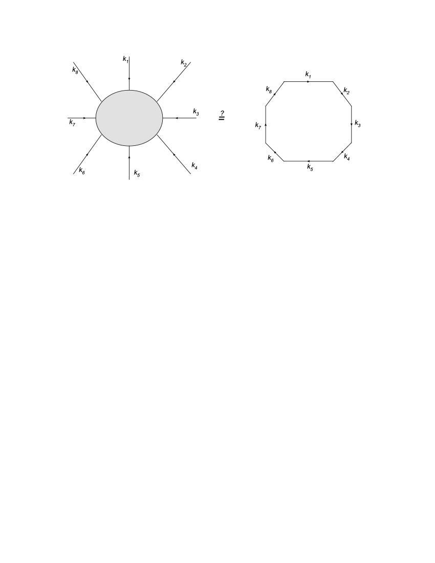
Figure 1: The general, conjectured, correspondence between gluon scattering amplitudes and Wilson loops associates edges of the Wilson loop to momenta of gluons. It was shown to hold at one loop for any number of external legs [3].

.

Physically, we expect that the only important diagrams involve edges corresponding to the collinear gluons and, at most, their closest neighbors. We can argue that this is correct by emphasizing, first, that the Splitting function is universal. Hence, generic diagrams connecting one of the collinear gluons with a far away line should decouple in the collinear limit. We will show that this is indeed correct in the sequel. Concerning the two adjacent lines to the collinear pair of gluons, it turns out that they don’t decouple in a trivial manner.

The divergent terms of gluon scattering amplitudes correspond, in the Wilson loop language (at one loop), to propagators between two adjacent edges. In the collinear limit there are interesting contributions from small changes in the angle of the two cusps $\{l_{1},v_{1}\}$ and $\{v_{2},l_{2}\}$ (see figure 2 for the notations). This effect accounts for many of the terms in (7). To evaluate these systematically, we write first

$$r_{S}^{(1)}=(M_{n}^{(1)}-M_{n-1}^{(1)})\bigg{|}_{\text{collinear limit}}=(I_{n}^{(1)}-I_{n-1}^{(1)})\bigg{|}_{\text{collinear limit}}+(F_{n}^{(1)}-F_{n-1}^{(1)})\bigg{|}_{\text{collinear limit}},$$

where $I$ and $F$ are the divergent and finite parts, respectively. The contribution from $(I_{n}^{(1)}-I_{n-1}^{(1)})\bigg{|}_{\text{collinear limit}}$ is as follows ($v_{1}$ and $v_{2}$ are collinear and $v\equiv v_{1}+v_{2}$)

$$(I_{n}^{(1)}-I_{n-1}^{(1)})\bigg{|}_{\text{collinear limit}}=\frac{-1}{2\epsilon^{2}}\biggl{(}(\frac{\mu^{2}}{-2l_{1}\cdot v_{1}})^{\epsilon}+(\frac{\mu^{2}}{-2v_{1}\cdot v_{2}})^{\epsilon}+(\frac{\mu^{2}}{-2v_{2}\cdot l_{2}})^{\epsilon}$$ (8)

$$-(\frac{\mu^{2}}{-2l_{1}\cdot v})^{\epsilon}-(\frac{\mu^{2}}{-2v\cdot l_{2}})^{\epsilon}\biggr{)}=$$ (9)

$$=\frac{-1}{2\epsilon^{2}}\biggl{(}(\frac{\mu^{2}}{-s})^{\epsilon}-(1-z^{-\epsilon})(\frac{\mu^{2}}{-2l_{1}\cdot v})^{\epsilon}-(1-(1-z)^{-\epsilon})(\frac{\mu^{2}}{-2l_{2}\cdot v})^{\epsilon}\biggr{)}=$$ (10)

$$=\frac{-1}{2\epsilon^{2}}(\frac{\mu^{2}}{-s})^{\epsilon}+\frac{1}{2\epsilon}\left(\ln(z)-\frac{\epsilon}{2}(\ln(z))^{2}\right)(\frac{\mu^{2}}{-2l_{1}\cdot v})^{\epsilon}+\frac{1}{2\epsilon}\left(\ln(1-z)-\frac{\epsilon}{2}(\ln(1-z))^{2}\right)(\frac{\mu^{2}}{-2l_{2}\cdot v})^{\epsilon},$$ (11)

where we have ignored $O(\epsilon)$ terms in our final expression, as we do everywhere in the sequel. Note that in the first equality the result is still exact and the collinear limit is taken only in the subsequent manipulations. The divergent terms as $\epsilon\rightarrow 0$ in

$$(I_{n}^{(1)}-I_{n-1}^{(1)})\bigg{|}_{\text{collinear limit}},$$

agree with those in $r_{S}^{(1)}$ (7), which is just a simple consistency check. The finite parts should combine with the ones from

$$(F_{n}^{(1)}-F_{n-1}^{(1)})\bigg{|}_{\text{collinear limit}},$$

to give the correct $r_{S}^{(1)}$. Finite parts arise in the Wilson loop computation from diagrams between non adjacent edges. The point is that there are only two non trivial diagrams contributing the missing finite parts of the collinear Splitting function, $\{l_{1},v_{2}\}$ and $\{v_{1},l_{2}\}$, depicted in figure 2.

Figure 2: The two contributions at one loop to the difference of finite parts in the collinear limit.

.

The exact computation of any one loop diagram was conducted in [3]. In our case, there is an immediate simplification due to the fact that these are really one-mass easy box functions (the general case includes two-mass easy box functions). Upon applying the collinear limit and dealing with the kinematics we arrive at the following expression ($v_{1}\sim z(v_{1}+v_{2})\equiv zv$) for the finite part

$$-Li_{2}\left(1+\frac{2zv\cdot l_{2}}{v^{2}}\right)-Li_{2}\left(1+\frac{2(1-z)v\cdot l_{1}}{v^{2}}\right)-Li_{2}\left(1+\frac{z}{1-z}\right)-Li_{2}\left(1+\frac{1-z}{z}\right)+$$ (12)

$$+Li_{2}\left(1+\frac{z(v^{2}+2v\cdot l_{2})}{(1-z)v^{2}}\right)+Li_{2}\left(1+\frac{(1-z)(v^{2}+2v\cdot l_{1})}{zv^{2}}\right),$$ (13)

where $Li_{2}$ is the famous Dilogarithm of Euler. This can be further simplified in the collinear limit by noting that the definition of the collinear limit is equivalent to $v^{2}\ll v\cdot l_{1}$ and $v^{2}\ll v\cdot l_{2}$. Thus the contribution of the two one loop diagrams is

$$-Li_{2}\left(\frac{2zv\cdot l_{2}}{v^{2}}\right)-Li_{2}\left(\frac{2(1-z)v\cdot l_{1}}{v^{2}}\right)-Li_{2}\left(1+\frac{z}{1-z}\right)-Li_{2}\left(1+\frac{1-z}{z}\right)+$$ (14)

$$+Li_{2}\left(\frac{2zv\cdot l_{2}}{(1-z)v^{2}}\right)+Li_{2}\left(\frac{2(1-z)v\cdot l_{1}}{zv^{2}}\right).$$ (15)

An identity by Euler

$$Li_{2}(z)+Li_{2}(1/z)+\frac{1}{2}\log^{2}(-z)+\pi^{2}/6=0,$$

implies that for $|z|\gg 1$

$$Li_{2}(z)=-\frac{1}{2}\log^{2}(-z)-\pi^{2}/6+O(z).$$

Another identity we need to use is

$$Li_{2}(z)+Li_{2}(1-z)=-\log(z)\log(1-z)+\pi^{2}/6.$$

With these relations (14) becomes (up to an additive constant)

$$2(F_{n}^{(1)}-F_{n-1}^{(1)})\bigg{|}_{\text{collinear limit}}=$$ (16)

$$=\frac{1}{2}\Biggl{(}\ln^{2}\left(-\frac{-2zv\cdot l_{2}}{-v^{2}}\right)+\ln^{2}\left(-\frac{-2(1-z)v\cdot l_{1}}{-v^{2}}\right)-\ln^{2}\left(-\frac{-2zv\cdot l_{2}}{-(1-z)v^{2}}\right)-\ln^{2}\left(-\frac{-2(1-z)v\cdot l_{1}}{-zv^{2}}\right)+$$ (17)

$$+\ln^{2}(-1/(1-z))+\ln^{2}(-1/z)-\ln(z)\ln(1-z)\Biggr{)}=$$ (18)

$$=\ln(1-z)\ln\left(\frac{-2zv\cdot l_{2}}{-v^{2}}\right)+\ln(z)\ln\left(\frac{-2(1-z)v\cdot l_{1}}{-v^{2}}\right)-\ln(z)\ln(1-z)=$$ (19)

$$=\ln(z)\ln(1-z)+\ln(1-z)\ln\left(\frac{-2v\cdot l_{2}}{-v^{2}}\right)+\ln(z)\ln\left(\frac{-2v\cdot l_{1}}{-v^{2}}\right).$$ (20)

One has to be a little careful in the manipulations leading to the last line, the imaginary parts cancel neatly and the result in the end is real. Adding this result to the one for the contribution to the Splitting amplitude from the the divergent piece, the dependence on $l_{1}$ and $l_{2}$ cancels very nicely and we are left precisely with the expected form of the one-loop Splitting function.

We see that in a very geometrical manner, Wilson loops exhibit a decoupling of the collinear region from the rest of the gluons. The non trivial part is to deal with the neighboring adjacent lines, where both the non trivial $z$ dependence resides and where the non trivial cancelation of the $l_{1},l_{2}$ dependence occurs. The cancelation of $l_{1},l_{2}$ is absolutely necessary for factorization and for the consistency of our procedure.

3.2 Strong coupling aspects

In appendix A we show that the finite part of the minimal area surface corresponding to gluons scattering matrix elements at strong coupling has to satisfy the following anomalous Ward identity

$$\sum_{i}\hat{K}_{i}^{\mu}F_{n}=\frac{\sqrt{\lambda}}{4\pi}\sum_{i=1}^{n}(x^{\mu}_{i-1}+x^{\mu}_{i+1}-2x_{i}^{\mu})\ln\left(s_{i,i+1}\right).$$ (21)

In the equation above,

$$\sum_{i}\hat{K}_{i}^{\mu}=\sum_{i}(2x_{i}^{\mu}(x_{i}\cdot\partial_{i})-x_{i}^{2}\partial_{i}^{\mu}),$$ (22)

$x_{i}$ are the coordinates of the cusps and $\lambda$ is the ’t Hooft coupling constant. This equation shows explicitly that the results of [5] hold in the strong coupling regime, as one may expect. This constraint fixes, up to a constant, four and five point functions. In these two cases, the solutions of this constraint coincide with the suggestion by BDS [6], again, up to a possible overall coefficient. Thus, the Splitting function coming from the difference of a pentagon and the quadrangle coincides with the prediction of [6] to the Splitting function at strong coupling (which is roughly (7) exponentiated with a pre-factor of the cusp anomalous dimension).

Since at strong coupling we are computing the minimal area of surfaces with prescribed boundary conditions, it is reasonable to expect that a flattened cusp will modify the surface only locally. In other words, we expect a factorization of Wilson loops at strong coupling in the collinear limit simply because the collinear limit modifies the minimal surface only slightly (It would be nice to construct a rigorous proof of this intuitive claim.). This argument implies that the Splitting function at strong coupling coincides with the one predicted by BDS, although their ansatz fails in general [8]. Qualitatively, an analogous situation is happening at two loops [9] where the Splitting function was observed to coincide with the prediction of BDS but the complete ansatz fails beyond the collinear limit.

4 Multi Splitting function

4.1 One loop aspects

One may also consider $2K$ adjacent gluons with momenta $\{v_{i}|i=1...2K\}$ such that $v_{i}\cdot v_{j}$ is smaller than all the other invariant (involving at least one gluon not from the set above) for all $i,j$. Namely, $2K$ adjacent collinear gluons. This is possible to do, but the computation is cumbersome and the analysis at strong coupling is less straightforward. Thus, we shall consider a special case where there are $2K$ collinear gluons whose momenta are distributed in a periodic fashion $v_{1},v_{2},v_{1},v_{2},...,v_{1},v_{2}$. This situation is depicted in figure 3.

Figure 3: The type of Wilson loop we consider. $v_{1}$ and $v_{2}$ are in the collinear limit and the lines $l_{1}$ and $l_{2}$ are the adjacent lines to the sequence of collinear gluons.

Our first goal is to determine the multi Splitting function at one loop for such a configuration using the technique we applied for the Splitting function of two gluons in the previous section. Again, diagrams connecting a generic gluon with any $v_{1}$ or $v_{2}$ average out as in the Splitting function of two gluons case and are, consequently, not important for the Splitting function. The subtlety is with the edges $l_{1},l_{2}$ which are crucial, for the same reasons as in the Splitting function of two gluons, in order to reproduce the correct Splitting function. We denote $v_{1}\simeq z(v_{1}+v_{2})\equiv zv$. Our notation would be that $p,q$ are the respective momenta of edges the gluon connects to, $P$ is the overall momentum of gluons interpolating from $p$ to $q$ and $P+Q+p+q=0$. We will also use $s=(p+P)^{2}$, $t=(q+P)^{2}$. For a demonstration of these notations see figure 4.

Figure 4: The definitions of $p,q,P,Q,s,t$ applied for a one loop contribution to a hexagon Wilson loop. Solid lines are part of the contour defining the Wilson loop and the dashed lines just denote some effective momenta.

Contributions from collinear - collinear diagrams

Potentially, there are contributions from diagrams where the gluon stretches along the sequence of collinear lines. These turn out to have no non trivial kinematical information. To see it we evaluate such diagrams explicitly. Consider, for instance, the case (where we use the notation $k\in\mathbb{N}$)

$$P=kv+v_{2},\hskip 10.00002ptp=q=v_{1}.$$ (23)

Obviously such diagrams vanish due to the fact they are proportional to the scalar product $v_{1}^{2}$. The less trivial case is

$$P=kv,\hskip 10.00002ptp=v_{2},\hskip 10.00002ptq=v_{1}.$$

It turns out that the quantity defined by

$$\bar{a}\equiv\frac{P^{2}+Q^{2}-s-t}{P^{2}Q^{2}-st}$$

diverges and we can not use the formulae of [3] to evaluate the finite part. Instead, we solve the integral explicitly and get

$$v^{2}\int_{[0,1]^{2}}d\tau_{p}d\tau_{q}\frac{1}{\left(k^{2}v^{2}+kv^{2}(\tau_{p}+\tau_{q})+v^{2}\tau_{p}\tau_{q}\right)^{1+\epsilon}}=$$

$$=(v^{2})^{-\epsilon}\int_{[0,1]^{2}}d\tau_{p}d\tau_{q}\frac{1}{\left((k+\tau_{p})(k+\tau_{q})\right)^{1+\epsilon}}=(v^{2})^{-\epsilon}\left(\ln\left(\frac{k+1}{k}\right)\right)^{2}.$$

Clearly, in the formal $\epsilon$ expansion we are doing here, this contribution is a constant which we are going to ignore anyway. We are interested only in a non trivial dependence on $z$, and these diagrams have no such.

Contributions from adjacent line - collinear diagrams

As we have already learnt, these are the important diagrams, eventually, giving rise to a non trivial multi Splitting function. There are actually four types of diagrams. I and II are diagrams stretching from $l_{1}$ to the sequence of collinear lines (ending on $v_{1}$,$v_{2}$ respectively) and III and IV are diagrams stretching from $l_{2}$ (ending on $v_{2}$,$v_{1}$ respectively). The computation of all these contributions is lengthy but straightforward. III and IV can be inferred from I and II by simple substitutions. The result is a sum over $k$ going from $1$ to $K-1$, counting the number of $v_{1},v_{2}$ pairs the gluon line has enclosed. In addition, two terms corresponding to one mass easy box functions identical in form to the contributions to the Splitting function of two gluons have to be included. We also employ the collinear limit to get rid of some terms. After some of the dust settles down the result is

$$2(F_{n+2K}^{(1)}-F_{n+1}^{(1)})\bigg{|}_{\text{collinear limit}}=$$

$$\text{Li}_{2}(\frac{v_{2}\cdot l_{1}}{v^{2}v_{1}\cdot l_{1}}2v\cdot l_{1})-\text{Li}_{2}(2\frac{v_{2}\cdot l_{1}}{v^{2}})-\text{Li}_{2}(1+\frac{v_{2}\cdot l_{1}}{v_{1}\cdot l_{1}})+\text{Li}_{2}(\frac{v_{1}\cdot l_{2}}{v^{2}v_{2}\cdot l_{2}}2v\cdot l_{2})-\text{Li}_{2}(2\frac{v_{1}\cdot l_{2}}{v^{2}})-\text{Li}_{2}(1+\frac{v_{1}\cdot l_{2}}{v_{2}\cdot l_{2}})$$

$$+\sum_{k=1}^{K-1}\Biggl{\{}\text{Li}_{2}(\frac{v_{1}\cdot l_{1}}{k^{2}v^{2}v_{2}\cdot l_{1}}(2kv\cdot l_{1}+2v_{1}\cdot l_{1}))-\text{Li}_{2}(\frac{v_{1}\cdot l_{1}}{kv^{2}v_{2}\cdot l_{1}}(2v\cdot l_{1}))-$$

$$-\text{Li}_{2}(1+\frac{v_{1}\cdot l_{1}}{kv_{2}\cdot l_{1}}(k+1))+\text{Li}_{2}(1+\frac{v_{2}\cdot l_{1}}{(k+1)v_{1}\cdot l_{1}}k)+\text{Li}_{2}(\frac{v_{2}\cdot l_{1}}{(k+1)v^{2}v_{1}\cdot l_{1}}(2v\cdot l_{1}))-$$

$$-\text{Li}_{2}(\frac{v_{2}\cdot l_{1}}{(k+1)^{2}v^{2}v_{1}\cdot l_{1}}(2kv\cdot l_{1}+2v_{1}\cdot l_{1}))+\text{Li}_{2}(\frac{v_{2}\cdot l_{2}}{k^{2}v^{2}v_{1}\cdot l_{2}}(2kv\cdot l_{2}+2v_{2}\cdot l_{2}))-$$

$$-\text{Li}_{2}(\frac{v_{2}\cdot l_{2}}{kv^{2}v_{1}\cdot l_{2}}(2v\cdot l_{2}))-\text{Li}_{2}(1+\frac{v_{2}\cdot l_{2}}{kv_{1}\cdot l_{2}}(k+1))+\text{Li}_{2}(1+\frac{v_{1}\cdot l_{2}}{(k+1)v_{2}\cdot l_{2}}k)+$$

$$+\text{Li}_{2}(\frac{v_{1}\cdot l_{2}}{(k+1)v^{2}v_{2}\cdot l_{2}}(2v\cdot l_{2}))-\text{Li}_{2}(\frac{v_{1}\cdot l_{2}}{(k+1)^{2}v^{2}v_{2}\cdot l_{2}}(2kv\cdot l_{2}+2v_{2}\cdot l_{2}))\Biggr{\}}.$$

This looks cumbersome but there are still many cancelations to take place and the collinear limit was not yet fully utilized. Our next step is to turn all the dilogarithms with large arguments into double logarithms and use the relations $v_{1}\sim zv$, $v_{2}\sim(1-z)v$.

$$2(F_{n+2K}^{(1)}-F_{n+1}^{(1)})\bigg{|}_{\text{collinear limit}}=$$ (24)

$$\ln(z)\ln(1-z)+\ln(1-z)\ln\left(\frac{-2v\cdot l_{2}}{-v^{2}}\right)+\ln(z)\ln\left(\frac{-2v\cdot l_{1}}{-v^{2}}\right)$$ (25)

$$-\frac{1}{2}\sum_{k=1}^{K-1}\Biggl{\{}\ln^{2}(\frac{-2z(k+z)v\cdot l_{1}}{(1-z)k^{2}v^{2}})-\ln^{2}(\frac{-2zv\cdot l_{1}}{(1-z)kv^{2}})+\ln^{2}(\frac{-2(1-z)v\cdot l_{1}}{z(k+1)v^{2}})-$$ (26)

$$-\ln^{2}(\frac{-2(1-z)(k+z)v\cdot l_{1}}{z(k+1)^{2}v^{2}})+\ln^{2}(\frac{-2(1-z)(k+1-z)v\cdot l_{2}}{zk^{2}v^{2}})-\ln^{2}(\frac{-2(1-z)v\cdot l_{2}}{zkv^{2}})+$$ (27)

$$+\ln^{2}(\frac{-2zv\cdot l_{2}}{(1-z)(k+1)v^{2}})-\ln^{2}(\frac{-2z(k+1-z)v\cdot l_{2}}{(1-z)(k+1)^{2}v^{2}})\Biggr{\}}$$ (28)

$$+\sum_{k=1}^{K-1}\Biggl{\{}\text{Li}_{2}(1+\frac{(1-z)k}{z(k+1)})-\text{Li}_{2}(1+\frac{(1-z)(k+1)}{zk})+\text{Li}_{2}(1+\frac{zk}{(1-z)(k+1)})-\text{Li}_{2}(1+\frac{z(k+1)}{(1-z)k})\Biggr{\}}.$$ (29)

To decipher the physical meaning of this result, we first collect the $l_{1},l_{2}$ dependence which gives our expression, after some algebra, the following form

$$2(F_{n+2K}^{(1)}-F_{n+1}^{(1)})\bigg{|}_{\text{collinear limit}}=\ln\left(\frac{1-z}{K}\right)\ln\left(\frac{-2v\cdot l_{2}}{-v^{2}}\right)+\ln\left(\frac{z}{K}\right)\ln\left(\frac{-2v\cdot l_{1}}{-v^{2}}\right)+\Psi(z,K),$$ (30)

where the function $\Psi(z,K)$ is independent, by definition, of $l_{1},l_{2}$. We can simplify it a little and write it as (We disregard $z$ independent constants, even if they depend on $K$. One could easily keep track of them if needed.)

$$\Psi(z,K)=$$ (31)

$$=\ln(z)\ln(1-z)-2\sum_{k=1}^{K-1}\Biggl{\{}\ln(\frac{z}{1-z})\ln(\frac{k+z}{k+1-z})+\ln((k+1-z)(k+z))\ln(\frac{k+1}{k})\Biggr{\}}$$ (32)

$$+\Re\sum_{k=1}^{K-1}\Biggl{\{}\text{Li}_{2}(1+\frac{(1-z)k}{z(k+1)})-\text{Li}_{2}(1+\frac{(1-z)(k+1)}{zk})+\text{Li}_{2}(1+\frac{zk}{(1-z)(k+1)})-\text{Li}_{2}(1+\frac{z(k+1)}{(1-z)k})\Biggr{\}}.$$ (33)

In order to derive the equation above, we had to make sure all the imaginary contributions neatly cancel, as in the case of the Splitting function of two gluons (Note we take the real part of the second sum in (31).).

Inspecting the dependence on $l_{1},l_{2}$ in equation (30) we see that this is exactly what we expect to get in order for the complete Splitting function to be universal. Namely, upon adding to (30) the contribution of the (difference of) divergent parts, we obtain an expression independent of $l_{1},l_{2}$. To see how it comes about, recall again that the divergent part at one loop takes the form

$$\mathcal{M}_{n}^{(1)}|_{div.}=\frac{-1}{2\epsilon^{2}}\sum_{i=1}^{n}\left(\frac{\mu^{2}}{-s_{i,i+1}}\right)^{\epsilon}.$$ (34)

In our case, of an almost light like vector $Kv$, $\mathcal{M}_{n}^{(1)}|_{div.}-\mathcal{M}_{n-1}^{(1)}|_{div.}$ takes the form

$$\frac{-1}{2\epsilon^{2}}\left(\frac{\mu^{2}}{-2v\cdot l_{1}}\right)^{\epsilon}\left(z^{-\epsilon}-K^{-\epsilon}\right)+\frac{-1}{2\epsilon^{2}}\left(\frac{\mu^{2}}{-2v\cdot l_{2}}\right)^{\epsilon}\left((1-z)^{-\epsilon}-K^{-\epsilon}\right)-\frac{2K-1}{2\epsilon^{2}}\left(\frac{\mu^{2}}{-v^{2}}\right)^{\epsilon}.$$ (35)

Upon expanding it in $\epsilon$, we discover that combined with (30) the dependence on the momenta $l_{1}$ and $l_{2}$ cancels and we remain with the expression for the multi Splitting function of this periodic sequence of collinear gluons.

We turn to investigating some properties of $\Psi(z,K)$. A trivial consistency check is that $\Psi(z,K)=\Psi(1-z,K)$. A more interesting exercise is to check some aspects of the large $K$ behavior dependence of $\Psi(z,K)$. The objective is to compare this result to the strong coupling behavior. To accomplish this, we study more carefully the summands defining $\Psi(z,K)$ in (31)

$$\Re\biggl{\{}-2\biggl{(}\ln\left(\frac{z}{1-z}\right)\ln\left(\frac{1+z/k}{1+(1-z)/k}\right)+\ln\left((1+z/k)(1+(1-z)/k)\right)\ln\left(1+1/k\right)\biggr{)}-$$ (36)

$$-\text{Li}_{2}\left(1+\frac{z(1+1/k)}{(1-z)}\right)+\text{Li}_{2}\left(1+\frac{(1-z)}{z(1+1/k)}\right)-\text{Li}_{2}\left(1+\frac{(1-z)(1+1/k)}{z}\right)+$$ (37)

$$+\text{Li}_{2}\left(1+\frac{z}{(1-z)(1+1/k)}\right)\biggr{\}}.$$ (38)

We have rewritten it in a way which enables to extract the large $k$ behavior easily. It is easy to see that the zeroth order in the $1/k$ expansion vanishes. Thus, there is no term linear in $K$ in $\Psi(z,K)$. It is less trivial but also straightforward (using $\text{Li}_{2}(x)^{\prime}=-\ln(1-x)/x$) to see that next term in the expansion, proportional to $1/k$, cancels as well. Consequently, there is no term going like $\ln(K)$ in $\Psi(z,K)$.

The next, $1/k^{2}$ term, does not vanish but contains no $z$ dependence, so it is just a constant contribution. The first non trivial term comes from the expansion to third order in $1/k$. This gives rise to a behaviour at large k of the form

$$\Psi(z,K)=\ln(z)\ln(1-z)-\frac{2}{3}\sum_{k}^{K}\left(\frac{1}{k^{3}}z(1-z)+O(\frac{1}{k^{4}})\right),$$ (39)

where again some constant contribution from the third order was thrown away. This is convergent for large $K$, of course.

We conclude that the only possible dependence on $K$ at large K is $O(1)$. In particular, there is no non trivial dependence on $z$ scaling with $K$. This feature can be easily compared to the Splitting function at strong coupling.

We wish to make another important comment regarding (39). Clearly, it is different from the result one would have got had the collinear limit been taken successively (in which case there would have been a dependence on $z$ scaling with $K$). This is indeed the expected behavior because treating successively pairs of adjacent gluons inside the sequence is not a reliable expansion; one has to resum the expansion in $v^{2}$ and get back the complete propagator.

4.2 Strong coupling aspects

Let us first begin by studying the minimal surface whose boundary at infinity is given by a periodic sequence of $v_{1},v_{2}$ where $v_{1}$ and $v_{2}$ are two light like vector whose sum is time like. For definiteness we specify

$$ds^{2}=dx^{+}dx^{-}-\sum_{i=2}(dx^{i})^{2},$$

with $x^{\pm}=x^{0}\pm x^{1}$. We can always Lorentz transform $v_{1}$ to the form $(1,0,0...,0)$. Using Euclidean rotations in the transverse space we can bring $v_{2}$ to the subspace spanned by $x^{+},x^{-},x^{2}$. At this stage we have to investigate Lorentz transformations of $\mathbb{R}^{2,1}$ which leave the line $x^{+}$ invariant (but can re-scale it). There are two generators which have this property and using them we can transform any pair of vectors to a canonical one

$$\{(1,0,0),(\alpha,\beta,\sqrt{\alpha\beta})\}\ \rightarrow\ \{\sqrt{\beta}(1,0,0),\sqrt{\beta}(0,1,0)\}.$$

By further using the rescaling generator it follows that any pair of light like vectors whose sum is time like can be transformed to

$$\{(1,0,0),(0,1,0)\}.$$

Thus, it is sufficient to find the minimal surface ending on the sequence of vectors generated by $\{(1,0,0),(0,1,0)\}$, as depicted in figure 5. A closely related problem was considered in [8]. The only (inconsequential) difference is that their the surface is rotated by $90$ degrees, i.e the sum of the vectors is space like.

Figure 5: We have to look for a minimal surface ending (on the boundary of $AdS_{5}$) on such a periodic piecewise linear function.

Reading out some gross features of the solution of [8], we see that $x^{1}$ decays exponentially with the $AdS$ radius $r$ as (we use the Poincaré patch metric $ds^{2}\sim\frac{dx^{2}+dr^{2}}{r^{2}}$)

$$x^{1}(r)\sim e^{-r},$$

and because of scale and lorentz invariance, the zig-zag decays exponentially also for the original sequence $v_{1},v_{2}$ in the following way

$$e^{-\frac{r}{\sqrt{\left|v_{1}\cdot v_{2}\right|}}}.$$ (40)

The area is also easy to compute, up to an unknown constant (of order one) $C$,

$$\mathcal{A}\sim N\frac{\mu^{\epsilon}}{(v_{1}\cdot v_{2})^{\epsilon}}\left(\frac{1}{\epsilon^{2}}+\frac{1-\ln 2}{2\epsilon}+C\right)+O(\epsilon),$$ (41)

where $N=2K-1$ is just the number of cusps (which is infinite for a strictly infinite sequence).

If such a long sequence (large K) is made collinear and embedded in some Wilson loop (part of such a Wilson loop is depicted in figure 3), then the relative smallness of $v_{1}\cdot v_{2}$ insures that very quickly the zig-zag “defects” decay and one can replace the collinear lines by an effective single line, namely, there is factorization. It is interesting to ask what is the Splitting function. There are two effects contributing to it. The first just comes from (41), which indeed supplies terms we expect in the Splitting function since these are the correct divergences associated with adjacent gluons. The other kind of effects contributing to the Splitting function are, morally, edge effects. These are out of control (as they were in [8]), but we can clearly expect them not to contain any non-trivial $z$ dependence scaling with $K$. Hence, the Splitting function contains terms scaling with $K$ (exactly the ones we expect) and some non trivial terms remaining finite as $K\rightarrow\infty$ which we can not compute. This is the same situation as for the multi Splitting function at one loop, where the non trivial information is in the function $\Psi(z,K)$, which does not have (non trivial) terms scaling with $K$.

It will be interesting to understand better these edge effects and to compare the multi Splitting functions at strong coupling to those predicted by the BDS ansatz, this is left to future work.

5 More comments and possible generalization

A crucial point at one loop, manifest in the Feynman gauge we used, is that propagators from the collinear gluons to generic distant edges do not contribute to the Splitting function. The two adjacent edges, as we have shown above, are an exception. One can understand this qualitatively by noting that propagators from generic distant edges to the collinear ones are finite as $v^{2}\rightarrow 0$. Hence, we expect that the difference between a completely flattened cusp (straight line) and one which is almost flat goes to zero as $v^{2}\rightarrow 0$. This is indeed what happens at one loop. The two adjacent edges are exceptional because their contribution is not finite as $v^{2}\rightarrow 0$ due to the integration over the region where the propagator is light like. This is explicit, for instance, in equation (16). Therefore, it permits a non trivial dependence on $z$, as indeed happens.

It is not completely trivial to generalize this argument to two loops. The basic reason is that diagrams like figure 6 diverge. Hence, any such diagram where two of the gluons end on two adjacent collinear edges is expected to be large as $v^{2}\rightarrow 0$. At first sight, this ruins the argument completely since we can no longer examine a very restricted set of graphs to check whether there is factorization.

Figure 6: Such a diagram diverges. Both straight lines in the pictures are light like.

.

There is a well known way to correct this pathology. We can consider, instead, the axial gauge

$$n\cdot A=0,$$

with $n^{2}\neq 0$. It is easy to check that in this gauge the set of divergent diagrams is much simpler; they are all “localized” around cusp points [12], see also [5]. In this gauge it should be easier to prove, to all orders, that there is factorization. We expect that this is indeed the case (There is already numerical evidence [9] for factorization of hexagons at two loops.). It may be easy to show that generic edges decouple in the collinear limit, by the same token as at one loop. The decoupling of adjacent edges is probably more tricky and we leave this study to future work.

Appendix A An anomalous Ward identity at strong coupling

Let us define $AdS_{5}$ by the embedding coordinates

$$-X_{-1}^{2}-X_{0}^{2}+X_{1}^{2}+X_{2}^{2}+X_{3}^{2}+X_{4}^{2}=-1,$$

and we denote

$$X_{+}=X_{-1}+X_{4},\hskip 20.00003ptX_{-}=X_{-1}-X_{4}.$$

We also introduce the Poincaré coordinates

$$X^{\mu}=\frac{x^{\mu}}{r}\ ,\hskip 10.00002ptX_{+}=\frac{1}{r}\ ,\hskip 10.00002ptX_{-}=\frac{r^{2}+x^{\mu}x_{\mu}}{r}.$$

The signature used in this appendix is $(-,+,+,+)$ and $\mu=0,...,3$. The metric in Poincaré coordinates is

$$ds^{2}=\frac{dx^{2}+dr^{2}}{r^{2}},$$

where we set the overall scale to $1$. Inversion symmetry acts in these embedding coordinates as $X_{+}\leftrightarrow X_{-}$ and becomes the usual inversion in $4$ dimensions ($x^{\mu}\rightarrow x^{\mu}/x^{2}$) near the boundary of $AdS_{5}$. Special conformal transformations are realized as a combination of inversion translation and another inversion. A simple calculation gives the precise formulas for the action of a special conformal symmetry on the Poincaré patch coordinates

$$r^{\prime}=\frac{r}{1+2x\cdot\beta+\beta^{2}(r^{2}+x^{2})},$$ (42)

$$(x^{\prime})^{\mu}=\frac{x^{\mu}+(r^{2}+x^{2})\beta^{\mu}}{1+2x\cdot\beta+\beta^{2}(r^{2}+x^{2})}.$$ (43)

Consider a minimal area problem whose Dirichlet boundary condition at the boundary of the Poincaré patch is made of $n$ light like lines (with out-in-out-in… ordering)

$$S=\frac{\sqrt{\lambda}}{2\pi}\int du_{1}du_{2}\sqrt{det\left(\partial_{a}X^{\mu}\partial_{b}X^{\nu}G_{\mu\nu}\right)}.$$ (44)

This action is obviously invariant under any coordinate transformation which leaves the Poincaré metric invariant, in particular (42). Note that these are global transformations of the Nambu-Goto action, and leave $u_{1}$,$u_{2}$ intact.

However, there are divergences in the classical area problem, and the action is supposed to be regulated. In our context, one implements the gravitational version of Dimensional Regularization [1], where the Nambu-Goto action is slightly modified by changing the metric to

$$ds^{2}=\frac{\sqrt{\lambda_{D}c_{D}}}{r^{\epsilon}}(\frac{dy^{2}+dr^{2}}{r^{2}}),$$ (45)

with

$$\lambda_{D}=\frac{\lambda\mu^{2\epsilon}}{(4\pi e^{-\gamma})^{\epsilon}}\ ,\hskip 20.00003ptc_{D}=2^{4\epsilon}\pi^{3\epsilon}\Gamma(2+\epsilon).$$

Consequently, the Nambu-Goto action becomes

$$S=\frac{\sqrt{\lambda_{D}c_{D}}}{2\pi}\int du_{1}du_{2}\frac{1}{r^{\epsilon}}\sqrt{det\left(\partial_{a}X^{\mu}\partial_{b}X^{\nu}G_{\mu\nu}\right)}\equiv\frac{\sqrt{\lambda_{D}c_{D}}}{2\pi}\int du_{1}du_{2}\frac{\mathcal{L}_{\epsilon=0}}{r^{\epsilon}},$$ (46)

where the $G_{\mu\nu}$ inside the square root is the same as in the unregulated metric (namely that of a Poincaré patch). In order for this regulated action to be convergent, we need to take $\epsilon<0$.

Let us perform a special conformal transformation of the fields in the action. This takes the form (42) and leaves $\mathcal{L}_{\epsilon=0}$ invariant by construction. However, the regularized action changes and becomes

$$S^{\prime}=\frac{\sqrt{\lambda_{D}c_{D}}}{2\pi}\int du_{1}du_{2}\frac{\mathcal{L}_{\epsilon=0}}{r^{\epsilon}}\left(1+2x\cdot\beta+\beta^{2}(r^{2}+x^{2})\right)^{\epsilon}.$$ (47)

One may worry that perhaps it is necessary to take into account corrections to the solution of the equations of motion (since it is only a solution as long as $\epsilon=0$). The argument here goes in the same way as in [1], where it was explained that (to reproduce the finite parts) it is sufficient to make sure that it is $\epsilon$ corrected (to leading order) in the vicinity of cusps. We will be careful about this rather subtle point.

Let us study the modified action (47) and expand it in both $\epsilon$ and $\beta$ to learn how a small special conformal transformation modifies the regularized area of the solution. We begin by expanding in $\epsilon$

$$S^{\prime}=\frac{\sqrt{\lambda_{D}c_{D}}}{2\pi}\int du_{1}du_{2}\frac{\mathcal{L}_{\epsilon=0}}{r^{\epsilon}}\times$$ (48)

$$\times\left(1+\epsilon\ln\left(1+2x\cdot\beta+\beta^{2}(r^{2}+x^{2})\right)+\frac{1}{2}\epsilon^{2}\ln^{2}\left(1+2x\cdot\beta+\beta^{2}(r^{2}+x^{2})\right)+O(\epsilon^{3})\right).$$ (49)

We know that further corrections are unimportant since they are $O(\epsilon)$ in the final answer. Expanding in $\beta$ we see that the $\epsilon^{2}$ term in the expansion is also proportional to $\beta^{2}$ (which means it does not contribute to the anomalous Ward identity governing the variation under infinitesimal special conformal transformations). Hence, the relevant terms in $S^{\prime}$ are really

$$S^{\prime}=\frac{\sqrt{\lambda_{D}c_{D}}}{2\pi}\int du_{1}du_{2}\frac{\mathcal{L}_{\epsilon=0}}{r^{\epsilon}}\times$$ (50)

$$\times\left(1+\epsilon\ln\left(1+2x\cdot\beta+\beta^{2}(r^{2}+x^{2})\right)\right)+O(\beta^{2}).$$ (51)

Expanding the remaining logarithm to leading power in $\beta$ we get

$$S^{\prime}=\frac{\sqrt{\lambda_{D}c_{D}}}{2\pi}\int du_{1}du_{2}\frac{\mathcal{L}_{\epsilon=0}}{r^{\epsilon}}\left(1+2\epsilon x\cdot\beta\right)+O(\beta^{2})=$$ (52)

$$=S+2\epsilon\beta_{\mu}\frac{\sqrt{\lambda_{D}c_{D}}}{2\pi}\int du_{1}du_{2}\frac{\mathcal{L}_{\epsilon=0}}{r^{\epsilon}}x^{\mu}+O(\beta^{2}).$$ (53)

Thus, we can write our result so far as (we don’t mention the $O(\beta^{2})$ corrections in the sequel)

$$\delta_{\beta}S=2\epsilon\beta_{\mu}\frac{\sqrt{\lambda_{D}c_{D}}}{2\pi}\int du_{1}du_{2}\frac{\mathcal{L}_{\epsilon=0}}{r^{\epsilon}}x^{\mu}.$$ (54)

Let us figure out how to calculate the interesting terms from this integral. Note that $x^{\mu}$ is generically finite all over the solution, both in the bulk and boundary. Since $\delta_{\beta}S$ contains $\epsilon$ in front of the integral, there are no contributions form the bulk of the worldsheet (since they are $O(\epsilon)$). Consequently, there are contributions only from lines and cusps. Both of these are well understood in general since they contribute to the universal divergent parts of amplitudes.

Figure 7: Generic cusp at the boundary of some minimal surface.

.

Consider a cusp with the adjacent momenta being $k_{i},k_{i+1}$. The cusp is assumed to be at $x_{i}$ and the momentum $k_{i}$ begins at $x_{i-1}$ and $k_{i+1}$ ends at $x_{i+1}$ (see figure 7). We can always make rescalings and Lorentz transformations so to bring the cusp to some plane $Y_{+},Y_{-}$ where the boundary of the worldsheet spans $Y_{\pm}\in[0,1]$. $Y_{-}=0,Y_{+}=1$ maps to the beginning of the vector $k_{i}$ in the original frame and similarly $Y_{-}=1,Y_{+}=0$ maps to the endpoint of $k_{i+1}$. The integrand in the neighborhood of a single cusp was analyzed in [1, 13]. We may take advantage of these results and write the contribution to the variation from a single cusp in our case

$$\delta_{\beta}S_{i,i+1}=-2\epsilon\beta_{\mu}C(\epsilon)\frac{\sqrt{\lambda}}{8\pi}\sqrt{\frac{\mu^{2\epsilon}}{(s_{i,i+1})^{\epsilon}}}\int dY_{+}dY_{-}\frac{x_{(i)}^{\mu}(Y_{+},Y_{-})}{(Y_{+}Y_{-})^{1+\epsilon/2}},$$ (55)

where all we need to know about $C(\epsilon)$ is that

$$C(\epsilon)=1+\frac{1}{2}(1-\ln 2)\epsilon+O(\epsilon^{2}),$$

and $s_{i,i+1}=(k_{i}+k_{i+1})^{2}=(x_{i+1}-x_{i-1})^{2}$. It is important to emphasize that (55) includes the needed $\epsilon$ adjustments of the single cusp solution, so we don’t have to worry about this issue anymore. In the vicinity of cusps and lines $x^{\mu}$ follows its Dirichlet boundary condition (which is a piecewise linear function). Thus, we can write without loss of generality that for our single cusp contribution

$$x_{(i)}^{\mu}(Y_{+},Y_{-})=x^{\mu}_{i}+\eta_{(i)}Y_{+}+\theta_{(i)}Y_{-},$$

where $\eta$ and $\theta$ are some real numbers. The integral is easily solvable

$$\int dY_{+}dY_{-}\frac{x^{\mu}_{i}+\eta_{(i)}Y_{+}+\theta_{(i)}Y_{-}}{(Y_{+}Y_{-})^{1+\epsilon/2}}=$$ (56)

$$=x^{\mu}_{i}\int dY_{+}dY_{-}\frac{1}{(Y_{+}Y_{-})^{1+\epsilon/2}}+\eta_{(i)}\int dY_{+}dY_{-}\frac{(Y_{+})^{-\epsilon/2}}{(Y_{-})^{1+\epsilon/2}}+\theta_{(i)}\int dY_{+}dY_{-}\frac{(Y_{-})^{-\epsilon/2}}{(Y_{+})^{1+\epsilon/2}}=$$ (57)

$$=\frac{4x_{i}^{\mu}}{\epsilon^{2}}-\frac{4(\eta_{(i)}+\theta_{(i)})}{\epsilon(2-\epsilon)}.$$ (58)

We combine this factor with the rest needed for $\delta_{\beta}S_{i,i+1}$ to obtain

$$\delta_{\beta}S_{i,i+1}=-2\epsilon\beta_{\mu}C(\epsilon)\frac{\sqrt{\lambda}}{8\pi}\sqrt{\frac{\mu^{2\epsilon}}{(s_{i,i+1})^{\epsilon}}}\left(\frac{4x_{i}^{\mu}}{\epsilon^{2}}-\frac{4(\eta_{(i)}+\theta_{(i)})}{\epsilon(2-\epsilon)}\right)=$$ (59)

$$=-2\beta_{\mu}C(\epsilon)\frac{\sqrt{\lambda}}{2\pi}\sqrt{\frac{\mu^{2\epsilon}}{(s_{i,i+1})^{\epsilon}}}\left(\frac{x_{i}^{\mu}}{\epsilon}-\frac{\eta_{(i)}+\theta_{(i)}}{2-\epsilon}\right)=$$ (60)

$$=-2\beta_{\mu}C(\epsilon)\frac{\sqrt{\lambda}}{2\pi}\left(\frac{x^{\mu}_{i}}{\epsilon}+x_{i}^{\mu}\ln\left(\frac{\mu}{\sqrt{s_{i,i+1}}}\right)-\frac{\eta_{(i)}+\theta_{(i)}}{2}+O(\epsilon)\right),$$ (61)

where we have expanded to the significant powers of $\epsilon$. To obtain the total variation we are required to sum over $i$

$$\delta_{\beta}S=-2\beta_{\mu}C(\epsilon)\frac{\sqrt{\lambda}}{2\pi}\sum_{i=1}^{n}\left(\frac{x^{\mu}_{i}}{\epsilon}+x_{i}^{\mu}\ln\left(\frac{\mu}{\sqrt{s_{i,i+1}}}\right)-\frac{\eta_{(i)}+\theta_{(i)}}{2}\right).$$ (62)

The fact we keep only the significant orders in $\epsilon$ is implicit. The last term clearly cancels in the sum since the $n$-gon is closed so the sum of displacements of $x^{\mu}$ vanishes. Hence,

$$\delta_{\beta}S=-2\beta_{\mu}C(\epsilon)\frac{\sqrt{\lambda}}{2\pi}\sum_{i=1}^{n}\left(\frac{x^{\mu}_{i}}{\epsilon}+x_{i}^{\mu}\ln\left(\frac{\mu}{\sqrt{s_{i,i+1}}}\right)\right).$$ (63)

It can be rewritten in the following way,

$$\delta_{\beta}S=-2\beta_{\mu}C(\epsilon)\frac{\sqrt{\lambda}}{2\pi}\times$$ (64)

$$\times\sum_{i=1}^{n}\left(\frac{x^{\mu}_{i-1}+x^{\mu}_{i+1}}{2\epsilon}+\frac{1}{2}(x^{\mu}_{i-1}+x^{\mu}_{i+1})\ln\left(\frac{\mu}{\sqrt{s_{i,i+1}}}\right)-\frac{1}{2}(x^{\mu}_{i-1}+x^{\mu}_{i+1}-2x_{i}^{\mu})\ln\left(\frac{\mu}{\sqrt{s_{i,i+1}}}\right)\right).$$ (65)

The reason for this rewriting will become clear soon. There are three terms in the brackets of (64). To interpret the first two we note that given two vectors $y^{\mu}$, $x^{\mu}$, under a small special conformal transformation their distance squared transforms as follows

$$(y^{\prime}-x^{\prime})^{2}=(y-x)^{2}(1-2\beta_{\nu}(y^{\nu}+x^{\nu}))+O(\beta^{2}).$$

Recall that any $n$ gluon scattering amplitude has a universal divergent part given by a sum over cusps in the following way [13]

$$\mathcal{A}_{n}^{div}=-\sum_{i=1}^{n}\frac{C(\epsilon)}{\epsilon^{2}}\frac{\sqrt{\lambda}}{2\pi}\sqrt{\frac{\mu^{2\epsilon}}{(s_{i,i+1})^{\epsilon}}}.$$

So, some of the terms in (64) must be associated to the change from $\mathcal{A}_{n}^{div}$ to $\mathcal{A}_{n}^{{}^{\prime}\ div}$ due to the transformation of the invariants $s_{i,i+1}$. This is easily calculated to $O(\beta^{2})$ and we obtain

$$\mathcal{A}_{n}^{{}^{\prime}\ div}=-\sum_{i=1}^{n}\frac{C(\epsilon)}{\epsilon^{2}}\frac{\sqrt{\lambda}}{2\pi}\sqrt{\frac{\mu^{2\epsilon}}{(s_{i,i+1})^{\epsilon}}}\left(1-2\beta\cdot(x_{i-1}+x_{i+1})\right)^{-\epsilon/2}=$$ (66)

$$=-\sum_{i=1}^{n}\frac{C(\epsilon)}{\epsilon^{2}}\frac{\sqrt{\lambda}}{2\pi}\sqrt{\frac{\mu^{2\epsilon}}{(s_{i,i+1})^{\epsilon}}}\left(1+\epsilon\beta\cdot(x_{i-1}+x_{i+1})\right)=$$ (67)

$$=\mathcal{A}_{n}^{div}-2\beta C(\epsilon)\frac{\sqrt{\lambda}}{2\pi}\cdot\sum_{i=1}^{n}\frac{1}{2\epsilon}\sqrt{\frac{\mu^{2\epsilon}}{(s_{i,i+1})^{\epsilon}}}(x_{i-1}+x_{i+1})=$$ (68)

$$=\mathcal{A}_{n}^{div}-2\beta C(\epsilon)\frac{\sqrt{\lambda}}{2\pi}\cdot\sum_{i=1}^{n}\frac{x_{i-1}+x_{i+1}}{2\epsilon}\left(1+\epsilon\ln\left(\frac{\mu}{\sqrt{s_{i,i+1}}}\right)\right),$$ (69)

where in the last line we have kept only the terms significant in $\epsilon$, again. This manifestly reproduces the first two terms of (64). Ergo, the third term must be associated to a variation of the finite part of the amplitude.

Denote the finite part of an $n$ point function by $F_{n}$. Our results prove that it transforms as follows under a small special conformal transformation

$$\delta_{\beta}F_{n}=-\beta_{\mu}C(\epsilon)\frac{\sqrt{\lambda}}{2\pi}\sum_{i=1}^{n}\left((x^{\mu}_{i-1}+x^{\mu}_{i+1}-2x_{i}^{\mu})\ln\left(\frac{\sqrt{s_{i,i+1}}}{\mu}\right)\right).$$

Of course, the $\mu$ term cancels and it is natural to get rid of it since there are no $\mu$s in the finite parts by definition. In addition, $C=1$ to $O(\epsilon)$ which is all what we have in the finite parts. Hence, we rewrite it in the following form

$$\delta_{\beta}F_{n}=-\beta_{\mu}\frac{\sqrt{\lambda}}{4\pi}\sum_{i=1}^{n}(x^{\mu}_{i-1}+x^{\mu}_{i+1}-2x_{i}^{\mu})\ln\left(s_{i,i+1}\right).$$ (70)

It can also be presented as a differential equation by substituting

$$\delta_{\beta}=\beta_{\mu}\cdot\sum_{i}(-2x_{i}^{\mu}(x_{i}\cdot\partial_{i})+x_{i}^{2}\partial_{i}^{\mu}),$$

we get our final form for the anomalous Ward identity

$$\sum_{i}\hat{K}_{i}^{\mu}F_{n}=\frac{\sqrt{\lambda}}{4\pi}\sum_{i=1}^{n}(x^{\mu}_{i-1}+x^{\mu}_{i+1}-2x_{i}^{\mu})\ln\left(s_{i,i+1}\right).$$ (71)

Some immediate applications of this result are the fact that four and five point functions are uniquely fixed by this equation so this establishes the statement in [8] that five point functions at strong coupling are indeed consistent with the BDS guess [6].

We note that combining perturbation theory and strong coupling the equation can be written in general as

$$\sum_{i}(2x_{i}^{\mu}(x_{i}\cdot\partial_{i})-x_{i}^{2}\partial_{i}^{\mu})F_{n}=\frac{f(\lambda)}{4}\sum_{i=1}^{n}(x^{\mu}_{i-1}+x^{\mu}_{i+1}-2x_{i}^{\mu})\ln\left(s_{i,i+1}\right),$$ (72)

where $f(\lambda)$ is the cusp anomalous dimension. In [5] the same Ward identity was proven to hold to all orders of perturbation theory. Here we verify their relation at strong coupling.

Another comment we wish to make is that an analogous exercise to the one we did here can be repeated for the scaling symmetry. In that case, $r\rightarrow\xi r$ which implies that the area integral is multiplied by an overall constant $\xi^{-\epsilon}$. This can be easily seen to be completely absorbed by the divergent parts (where it rescales $s_{i,i+1}\rightarrow\xi^{2}s_{i,i+1}$ for any $i$). Thus, the finite part function satisfies

$$\sum_{i}x_{i}\cdot\partial_{i}F_{n}=0.$$

Similarly, it is annihilated by the Poincaré group (since the regulator preserves these symmetries).

References

- [1] L. F. Alday and J. Maldacena, “Gluon scattering amplitudes at strong coupling,” JHEP 0706, 064 (2007) [arXiv:0705.0303 [hep-th]].
- [2] J. M. Drummond, G. P. Korchemsky and E. Sokatchev, “Conformal properties of four-gluon planar amplitudes and Wilson loops,” arXiv:0707.0243 [hep-th].
- [3] A. Brandhuber, P. Heslop and G. Travaglini, “MHV Amplitudes in N=4 Super Yang-Mills and Wilson Loops,” arXiv:0707.1153 [hep-th].
- [4] J. M. Drummond, J. Henn, G. P. Korchemsky and E. Sokatchev, “On planar gluon amplitudes/Wilson loops duality,” arXiv:0709.2368 [hep-th].
- [5] J. M. Drummond, J. Henn, G. P. Korchemsky and E. Sokatchev, “Conformal Ward identities for Wilson loops and a test of the duality with gluon amplitudes,” arXiv:0712.1223 [hep-th].
- [6] Z. Bern, L. J. Dixon and V. A. Smirnov, “Iteration of planar amplitudes in maximally supersymmetric Yang-Mills theory at three loops and beyond,” Phys. Rev. D 72, 085001 (2005) [arXiv:hep-th/0505205].
- [7] M. Kruczenski, “A note on twist two operators in N = 4 SYM and Wilson loops in Minkowski signature,” JHEP 0212, 024 (2002) [arXiv:hep-th/0210115].
- [8] L. F. Alday and J. M. Maldacena, “Comments on gluon scattering amplitudes via AdS/CFT,” arXiv:0710.1060 [hep-th].
- [9] J. M. Drummond, J. Henn, G. P. Korchemsky and E. Sokatchev, “The hexagon Wilson loop and the BDS ansatz for the six-gluon amplitude,” arXiv:0712.4138 [hep-th].
- [10] Z. Bern, L. J. Dixon, D. C. Dunbar and D. A. Kosower, “One loop n point gauge theory amplitudes, unitarity and collinear limits,” Nucl. Phys. B 425, 217 (1994) [arXiv:hep-ph/9403226].
- [11] D. A. Kosower, “All-order collinear behavior in gauge theories,” Nucl. Phys. B 552, 319 (1999) [arXiv:hep-ph/9901201].
- [12] R. K. Ellis, H. Georgi, M. Machacek, H. D. Politzer and G. G. Ross, “Perturbation Theory And The Parton Model In QCD,” Nucl. Phys. B 152, 285 (1979). Y. L. Dokshitzer, D. Diakonov and S. I. Troian, “Hard Processes In Quantum Chromodynamics,” Phys. Rept. 58, 269 (1980).
- [13] E. I. Buchbinder, “Infrared Limit of Gluon Amplitudes at Strong Coupling,” arXiv:0706.2015 [hep-th].
- [14] Y. Oz, S. Theisen and S. Yankielowicz, arXiv:0712.3491 [hep-th]. H. Itoyama and A. Morozov, arXiv:0712.2316 [hep-th]. A. Jevicki, K. Jin, C. Kalousios and A. Volovich, arXiv:0712.1193 [hep-th]. H. Itoyama, A. Mironov and A. Morozov, arXiv:0712.0159 [hep-th]. K. Ito, H. Nastase and K. Iwasaki, arXiv:0711.3532 [hep-th]. G. Yang, arXiv:0711.2828 [hep-th]. A. Mironov, A. Morozov and T. Tomaras, arXiv:0711.0192 [hep-th]. R. Ricci, A. A. Tseytlin and M. Wolf, JHEP 0712, 082 (2007) [arXiv:0711.0707 [hep-th]]. A. Popolitov, arXiv:0710.2073 [hep-th]. D. Astefanesei, S. Dobashi, K. Ito and H. S. Nastase, JHEP 0712, 077 (2007) [arXiv:0710.1684 [hep-th]]. S. Ryang, arXiv:0710.1673 [hep-th]. J. McGreevy and A. Sever, arXiv:0710.0393 [hep-th]. R. Roiban and A. A. Tseytlin, JHEP 0711, 016 (2007) [arXiv:0709.0681 [hep-th]]. S. G. Naculich and H. J. Schnitzer, arXiv:0708.3069 [hep-th]. A. Mironov, A. Morozov and T. N. Tomaras, JHEP 0711, 021 (2007) [arXiv:0708.1625 [hep-th]]. A. Jevicki, C. Kalousios, M. Spradlin and A. Volovich, JHEP 0712, 047 (2007) [arXiv:0708.0818 [hep-th]]. L. F. Alday and J. M. Maldacena, JHEP 0711, 019 (2007) [arXiv:0708.0672 [hep-th]]. Z. Komargodski and S. S. Razamat, arXiv:0707.4367 [hep-th]. M. Kruczenski, R. Roiban, A. Tirziu and A. A. Tseytlin, Nucl. Phys. B 791, 93 (2008) [arXiv:0707.4254 [hep-th]]. S. Abel, S. Forste and V. V. Khoze, arXiv:0705.2113 [hep-th].