Solitons in two-dimensional Bose-Einstein condensates

Abstract

The excitations of a two-dimensional (2D) Bose-Einstein condensate in the presence of a soliton are studied by solving the Kadomtsev-Petviashvili equation which is valid when the velocity of the soliton approaches the speed of sound. The excitation spectrum is found to contain states which are localized near the soliton and have a dispersion law similar to the one of the stable branch of transverse oscillations of a 1D gray soliton in a 2D condensate. By using the stabilization method we show that these localized excitations behave as resonant states coupled to the continuum of free excitations of the condensate.

Bose-Einstein condensates of ultracold atoms are ideal systems for exploring matter wave solitons book . For most purposes, these condensates at zero temperature are well described by the Gross-Pitaevskii (GP) equation PG which has the form of a nonlinear Schrödinger equation, where nonlinearity comes from the interaction between atoms. In one dimension, the GP equation for condensates with repulsive interaction admits solitonic solutions corresponding to a local density depletion, namely gray and dark solitons. Such solitons have already been created and observed in elongated condensates with diverse techniques Burger .

Also multidimensional solitons in condensates have attracted much attention Brand . An interesting type of excitation in a two-dimensional (2D) condensate is represented by a self-propelled vortex-antivortex pair which is a particular solitonic solution of the GP equation Jones ; Jones2 ; Berloff ; Berloff2 . In the low momentum limit, the relation between the energy $E$ and momentum ${\bf P}$ of the soliton Jones approaches the dispersion law of Bogoliubov phonons, $\epsilon=cq$, from below. In this limit, when the 2D soliton moves at a velocity $V$ close to the Bogoliubov sound speed $c$, the phase singularities of the vortex-antivortex pair disappear and the soliton takes the form of a localized density depletion, also called rarefaction pulse. Moreover, if $V$ is close to $c$ the GP equation can be rewritten in a simpler form, known as the Kadomtsev-Petviashvili (KP) equation KP .

In a previous short paper Tsuchiya , we already presented some preliminary results on the dynamics and stability of this 2D soliton. In particular, we studied the excitations of the condensate in the presence of the soliton by linearizing the KP equation around the stationary solution. By looking at the shape of the eigenfunctions we found excitations localized near the soliton, having shape and dispersion law similar to those of the transverse oscillations of a 1D gray soliton in a 2D condensate. In this work we present a more systematic analysis. We use a stabilization method in order to obtain a better determination of the dispersion law of the localized states. Moreover, the same method allows us to visualize the coupling between the localized states and the free states, i.e., the Bogoliubov phonons of the uniform condensate.

Let us first summarize the derivation of the KP equation. We consider a 2D condensate with a soliton moving at a constant velocity $V$ in the $x$-direction. If the density at large distances is $n_{\infty}$, one can define the healing length $\xi=\hbar/[2mgn_{\infty}]^{1/2}$, where $g$ is the mean-field coupling constant and $m$ is the mass of the bosons. One can also introduce the dimensionless variables $x\to\xi x$, $y\to\xi y$, and $t\to mt\xi^{2}/\hbar$, the normalized order parameter $\Psi\to\sqrt{n_{\infty}}\Psi$, and the velocity $U=m\xi V/\hbar=V/(c\sqrt{2})$. In the frame moving with the soliton, the GP equation is Jones

$$2i\frac{\partial\Psi}{\partial t}=-\nabla^{2}\Psi+2iU\frac{\partial}{\partial x}\Psi+\left(|\Psi|^{2}-1\right)\Psi\;.$$ (1)

The order parameter can be written in the form $\Psi=n^{1/2}\exp[iS]$. The equations for the phase and the density thus become

$$\frac{\partial S}{\partial t} = \frac{1}{2}\frac{\nabla^{2}n^{1/2}}{n^{1/2}}-\frac{1}{2}\left(\nabla S\right)^{2}-\frac{1}{2}(n-1)+U\frac{\partial S}{\partial x}\;\;,$$ (2)

$$\frac{\partial n}{\partial t} = -(\nabla n)\cdot(\nabla S)-n(\nabla^{2}S)+U\frac{\partial n}{\partial x}\;\;.$$ (3)

When $V$ is close to $c$, one has $U\simeq 1/\sqrt{2}$. Let us introduce a small parameter $\varepsilon\equiv\sqrt{1-2U^{2}}$, so that $U\simeq 1/\sqrt{2}-1/(2\sqrt{2})\varepsilon^{2}$, and expand the density and the phase in this form

$$n = 1-\varepsilon^{2}f+\dots\;\;,$$ (4)

$$S = \varepsilon s+\dots\;\;.$$ (5)

To the lowest order in $\varepsilon$, the GP equation gives $\partial s/\partial x=-\varepsilon f/\sqrt{2}$ and

$$\frac{\partial}{\partial\tilde{x}}\left(\frac{\partial f}{\partial\tilde{t}}+6f\frac{\partial f}{\partial\tilde{x}}+\frac{\partial^{3}f}{\partial\tilde{x}^{3}}\right)=\frac{\partial^{2}f}{\partial\tilde{y}^{2}}\;\;,$$ (6)

where we have introduced the stretched variables $\tilde{x}=-\varepsilon x+\varepsilon^{3}t/(2\sqrt{2})$, $\tilde{y}=\varepsilon^{2}y/\sqrt{2}$ and $\tilde{t}=\varepsilon^{3}t/(4\sqrt{2})$. Equation (6) is known as the Kadomtsev-Petviashvili (KP) equation KP . Hereafter we will omit the tilde in the stretched variables.

The KP equation (6) admits a stationary solution of the form

$$f_{0}(x-2t)={\rm sech}^{2}\left[(x-2t)/\sqrt{2}\right]\;\;.$$ (7)

which is independent of $y$ and is a limiting form of a 1D gray soliton Tsuzuki . The linear stability of this gray soliton in two dimensions was studied in Zakharov ; Alexander . One can look for transverse fluctuations propagating along $y$ of the form $f(x,y,t)=f_{0}(x-2t)+\psi(x-2t)e^{i(ky-\omega t)}$ and solve the KP equation up to terms linear in $\psi$. One obtains the dispersion law

$$\omega^{2}=\frac{16}{3\sqrt{3}}k^{2}\left(k-\frac{\sqrt{3}}{2}\right)\;\;.$$ (8)

The frequency $\omega$ is real for $k\geq\sqrt{3}/2$ and imaginary for $k<\sqrt{3}/2$. The gray soliton (7) is thus unstable: long wavelength transverse oscillations can grow exponentially (snake instability). We note also that for $k\gg 1$ the stable branch of excitations behaves as $\omega\propto k^{3/2}$, similarly to the dispersion of capillary waves on the surface of a liquid.

The KP equation (6) admits also a 2D solitonic solution of the form Manakov

$$f_{0}(x-2t,y)=\frac{4[\frac{3}{2}+2y^{2}-(x-2t)^{2}]}{[\frac{3}{2}+2y^{2}+(x-2t)^{2}]^{2}}\;\;,$$ (9)

which corresponds to the $V\to c$ limit of the rarefaction pulse Jones . The function $f_{0}$ is plotted in Fig. 1. Differently from the 1D gray soliton (7), the solution (9) decays algebraically in all directions.

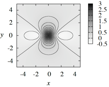
Figure 1: Solitonic solution (9) of the KP equation (6) as a function of the stretched dimensionless lengths $x$ and $y$ (see text for definitions). For a given value of the small parameter $\varepsilon$, the density distribution of the condensate is given by $n=1-\varepsilon^{2}f$ and the ratio between the soliton widths along $x$ and $y$, in dimensional units, scales as $\varepsilon$.

In the units of the GP equation (1), the density profile of the soliton is found by inserting Eq. (9) into Eq. (4). Its size along $x$ and $y$ is of the order of $1/\varepsilon$ and $1/\varepsilon^{2}$, respectively. To the first order in $\varepsilon$, the momentum $P$ and the energy $E$ per unit length are Jones

$$P=\frac{8\pi\sqrt{2}}{3}\hbar n_{\infty}\xi\varepsilon\;\;,\;\;E=\frac{8\pi}{3m}\hbar^{2}n_{\infty}\varepsilon=cP\;.$$ (10)

As it must be, the soliton has a sound-like dispersion in the limit where the KP equation is valid, that is, when $P\to 0$.

Now we consider density fluctuations of the form $f(x,y,t)=f_{0}(x-2t,y)+\psi(x-2t,y)e^{-i\omega t}$. Inserting this expression into Eq. (6) and keeping terms linear in $\psi$, we find

$$\frac{\partial^{4}\psi}{\partial x^{4}}+6\frac{\partial^{2}}{\partial x^{2}}\left(f_{0}\psi\right)-2\frac{\partial^{2}\psi}{\partial x^{2}}-\frac{\partial^{2}\psi}{\partial y^{2}}=i\omega\frac{\partial\psi}{\partial x}\;\;.$$ (11)

It is convenient to introduce the function $\phi(x,y)$ such that $\psi=\partial^{2}\phi/\partial x^{2}$. By integrating Eq. (11) twice in $x$, one has

$$\frac{\partial^{4}\phi}{\partial x^{4}}+6f_{0}\frac{\partial^{2}\phi}{\partial x^{2}}-2\frac{\partial^{2}\phi}{\partial x^{2}}-\frac{\partial^{2}\phi}{\partial y^{2}}=i\omega\frac{\partial\phi}{\partial x}\;\;.$$ (12)

We numerically solve this equation in a box of size $L_{x}\times L_{y}$. The function $\phi$ is expanded in plane waves with periodic boundary conditions: $\phi(x,y)=\sum_{\nu,\mu}\phi_{\nu\mu}\chi_{1,\nu}(x)\chi_{2,\mu}(y)$, with $\chi_{1,\nu}(x)=L_{x}^{-1/2}e^{i2\pi\nu x/L_{x}}$ for $|\nu|\leq l_{x}\;(\nu\neq 0)$. Concerning $\chi_{2,\mu}(y)$ we note that Eqs. (11) and (12) are invariant for $y\to-y$. Therefore the function $\phi$ is either an even or odd function of $y$. If it is even, then one can take $\chi_{2,\mu}(y)=(2/L_{y})^{1/2}\cos(2\pi\mu y/L_{y})$ for $1\leq\mu\leq l_{y}$ and $\chi_{2,0}(y)=(1/L_{y})^{1/2}$. If it is odd, one can take $\chi_{2,\mu}(y)=(2/L_{y})^{1/2}\sin(2\pi\mu y/L)$ for $1\leq\mu\leq l$. One thus obtains the following matrix equation

$$\left(-q_{x}^{3}-2q_{x}-\frac{q_{y}^{2}}{q_{x}}\right)\phi_{\nu\mu}+6\sum_{\nu^{\prime},\mu^{\prime}}\frac{(q_{x}^{\prime})^{2}}{q_{x}}M_{\nu\mu,\nu^{\prime}\mu^{\prime}}\phi_{\nu^{\prime}\mu^{\prime}}$$

$$=\omega\phi_{\nu\mu},$$ (13)

$$M_{\nu\mu,\nu^{\prime}\mu^{\prime}}=\!\int_{-L_{x}/2}^{L_{x}/2}\!dx\!\int_{-L_{y}/2}^{L_{y}/2}\!dy\ \chi_{1,\nu}^{\ast}\chi_{2,\mu}^{\ast}f_{0}\chi_{1,\nu^{\prime}}\chi_{2,\mu^{\prime}},$$ (14)

where $q_{x}=2\pi\nu/L_{x}$, $q_{y}=2\pi\mu/L$. The size of the matrix is $N\times N$, where $N=2l_{x}(l_{y}+1)$ for $\phi$ even, and $N=2l_{x}l_{y}$ for $\phi$ odd.

By solving Eq. (13), we find that all eigenvalues are real and positive. This is consistent with the stability of the 2D soliton Berloff ; Kuznetsov . As already discussed in Tsuchiya , among the eigenvectors we find states which are localized near the soliton. In order to better identify these states and explore their coupling with the free, unbound states we use a stabilization method Mandelshtam . In this method, the eigenvalues are calculated repeatedly for different box sizes $L_{y}$ and $L_{x}$. Once the frequency is plotted as a function of the box size, the localized states are identified as those having a dispersion which becomes flat for large boxes, larger than the typical size of the corresponding bound state. These states are immersed into a bath of unbound states. The latter are characterized by the number of nodes of the eigenfunctions in the $x$ and $y$ directions and, due to the finite box, they appear as series of discrete branches in the stabilization diagram. The dispersion laws of the unbound states, as well as their dependence on $L_{y}$ and $L_{x}$, can be estimated analytically by inserting $f_{0}=0$ into the equations (13) and (14). A coupling between bound (resonant) states and unbound (free) states can be seen in the stabilization diagram in the form of avoided crossings due to non-zero matrix elements connecting the two types of states Mandelshtam . A typical diagram is shown in Fig. 2, where we plot the eigenfrequencies of Eq. (13) as a function of $L_{y}$ for $L_{x}=10$. Flat dispersions and avoided crossing are clearly visible. An example of localized state is shown in Fig. 3, where we plot the $x=0$ section of the wave function of one of the bound states of Fig. 2 together with the soliton profile.

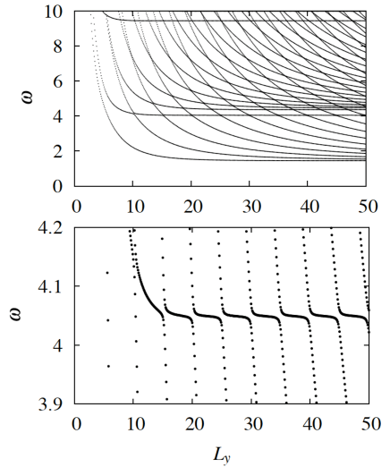
Figure 2: Eigenfrequencies $\omega$ of Eq. (13) as a function of $L_{y}$ for $L_{x}=10$. The lower plot is a magnification of the upper one around $\omega=4$. All quantities are dimensionless.

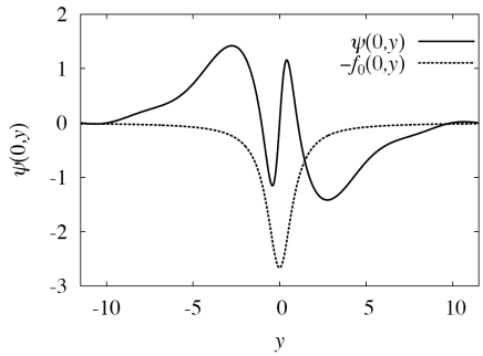
Figure 3: Wave function $\psi(0,y)$ (solid line) of an excited state localized near the soliton. The soliton profile, $-f_{0}(0,y)$, is shown as a dashed line. The excited state has frequency $\omega=4.05$ and the box size is $L_{x}=10$ and $L_{y}=23$. All quantities are dimensionless.

In the soliton region the wave function of the excited states exhibits oscillations in the $y$ direction whose wave vector $k$ can be easily estimated. It is interesting to plot the eigenfrequency $\omega$ of the bound states, extracted from the stabilization diagram, as a function of $k$, extracted from the shape of the corresponding wave functions. This is done in Fig. 4 for the bound states having the lowest number of nodes in the $x$ directions. Our results are shown as points with error bars, where the error bars are of the order of the inverse of the size of the soliton along $y$. In the same figure, the dispersion law (8) of the stable branch of excitations of a 1D gray soliton is plotted. The spectrum is very similar. This reflects the fact that a 2D soliton moving with velocity close to $c$ is very elongated in the $y$ direction (the ratio between the widths along $x$ and $y$, in dimensional units, is proportional to the small parameter $\varepsilon$) and its density distribution is indeed similar to that of a 1D gray soliton. Differently from a 1D gray soliton the 2D soliton has a discrete spectrum of bound states due to its finite length. This finite length also implies an “infrared cutoff” in the spectrum of the bound states, so that the long wavelength transverse oscillations of the infinite 1D soliton, which cause its snake instability, are not present in the spectrum of the 2D soliton.

The occurrence of a coupling between bound and unbound states, which is visible in the avoided crossings in the stabilization diagram, is worth stressing. The width of the avoided crossings is directly related to the lifetime of the bound (resonant) states associated with their decay into Bogoliubov sound modes. For typical resonant states, like the one in Fig. 2, we find a width of the resonance, $\Delta\omega$, of the order of $5\times 10^{-3}$ note . In Tsuchiya we noticed that the possible existence of bound states with infinite lifetime and dispersion law $\sim k^{3/2}$ could affect the thermodynamics of a 2D condensate. The present analysis suggests that the bound states of the 2D soliton have a finite lifetime, hence making the problem more complex.

Figure 4: Frequency of lowest excited states of the 2D soliton. Each point corresponds to an eigenvalue of the matrix equation (13), whose eigenfunction $\psi$ is localized in the soliton region and exhibits oscillations along $y$ with wave vector $k$. The solid line is the dispersion law of the stable branch of excitations of a 1D gray soliton in two dimensions, Eq. (8). All quantities are dimensionless.

In conclusion, a rarefaction pulse is an interesting solitonic excitation of a 2D condensate, which moves at velocity close to the Bogoliubov sound and is the low energy counterpart of a self-propelled vortex-antivortex pair. Its momentum and energy were calculated in Ref. Jones . The stability of the 2D rarefaction pulse in the KP limit was derived in Kuznetsov from the boundness of the Hamiltonian. It was also investigated in Jones2 , by means of both analytic arguments and numerical simulations. More recent numerical results on the linear stability have been reported in Berloff . However, a detailed calculation of the spectrum of the 2D condensate in the presence of the soliton has not yet been performed. In this work we have presented the results of such a calculation, including an analysis of resonant states based on a stabilization method. We have found localized states which closely resemble the stable branch of excitations of a 1D gray soliton. In the stabilization diagram, these states appear as resonant states coupled to the bath of unbound Bogoliubov phonons. We think that these results can be of interest for the investigation of ultracold bosonic gases in disk-shaped confining potentials, where vortex pairs are known to play a crucial role Hadzibabic . The observation of solitons in these systems would represent a nice manifestation of nonlinear dynamics in low dimensional superfluids.

We thank C. Tozzo, C. Lobo, P. Pedri, N. Prokof’ev, B. Svistunov, and N. Hatano for useful discussions.

References

- (1) L.P. Pitaevskii and S. Stringari, Bose-Einstein Condensation (Oxford, New York, 2003).
- (2) L.P. Pitaevskii, Sov. Phys. JETP 13, 451 (1961); E.P. Gross, Nuovo Cimento 20, 454 (1961).
- (3) S. Burger et al., Phys. Rev. Lett. 83, 5198 (1999); J. Denschlag et al., Science 287, 97 (2000); B.P. Anderson et al., Phys. Rev. Lett. 86, 2926 (2001); Z. Dutton et al., Science 293, 663 (2001); N.S. Ginsberg, J. Brand, and L.V. Hau, Phys. Rev. Lett. 94, 040403 (2005); P. Engels and C. Atherton, Phys. Rev. Lett. 99, 160405 (2007).
- (4) J. Brand, L.D. Carr, and B.P. Anderson, e-print arXiv:0705.1341; L.D. Carr, J. Brand, e-print arXiv:0705.1139.
- (5) C.A. Jones and P.H. Roberts, J. Phys. A: Math. Gen. 15, 2599 (1982).
- (6) C.A. Jones, S.J. Putterman, and P.H. Roberts, J. Phys. A: Math. Gen. 19, 2991 (1986).
- (7) N.G. Berloff and P.H. Roberts, J. Phys. A: Math. Gen. 37, 11333 (2004).
- (8) N.G. Berloff, J. Phys. A: Math. Gen. 37, 1617 (2004).
- (9) B.B. Kadomtsev and V.I. Petviashvili, Sov. Phys. Doklady 15, 539 (1970).
- (10) S. Tsuchiya, F. Dalfovo, C. Tozzo, and L. Pitaevskii, in “Proceedings of the 2006 International Conference on Quantum Fluids and Solids, Kyoto”, J. Low Temp. Phys. 148, 393 (2007).
- (11) T. Tsuzuki, J. Low Temp. Phys. 4, 441 (1971).
- (12) V.E. Zakharov, JETP Lett. 22, 172 (1975).
- (13) J.C. Alexander, R.L. Pego, and R.L. Sachs, Phys. Lett. A 226, 187 (1997).
- (14) S.V. Manakov et al., Phys. Lett. 63A, 205 (1977).
- (15) E.A. Kuznetsov and S.K. Turitsyn, Sov. Phys. JETP 55 844 (1982).
- (16) V.A. Mandelshtam, T.R. Ravuri, and H.S. Taylor, Phys. Rev. Lett. 70, 1932 (1993).
- (17) A more precise determination of the width and lifetime of the resonant states in our 2D geometry would require larger boxes and hence larger matrices, beyond the capability of our computation and the scope of this work.
- (18) Z. Hadzibabic et al., Nature 441, 1118 (2006); P. Krüger et al., Phys. Rev. Lett. 99, 040402 (2007); Z. Hadzibabic et al., e-print arXiv:0712.1265, and references therein.