Empirical Functionals for Reduced Density Matrix Functional Theory

Abstract

We present fully empirical exchange-correlation functionals to be used within reduced density matrix functional theory (RDMFT). These are of the popular J-K form, where the function of the occupation numbers that multiplies the Fock orbital term is written as a Padé approximant. The coefficients of the Padé are optimized for a test set of eight molecules, and then refined for a larger set of 35 molecules. Two different approaches were tried, either keeping the self-interaction terms, or by removing them explicitly from the functional. The functionals thus obtained involve very few parameters, but are able to outperform other RDMFT functionals, yielding correlation energies that are, on average, even slightly better than Møller-Plesset MP2 theory.

Reduced matrix density functional theory (RDMFT) has been emerging as an excellent tool for the study of correlation in molecular systems. It is based on Gilbert’s theoremgilbert , that asserts a one-to-one correspondence between the ground-state many-body wave function and the one-particle reduced density matrix, $\gamma$. Several theoretical advantages are immediately evident from using $\gamma$ instead of, e.g., the electronic density $\rho$ as in standard density functional theory (DFT): i) both the kinetic energy and the exchange energy can be trivially written as explicit functionals of $\gamma$; ii) consequently, the so-called correlation energy in RDMFT has a proper scaling with the strength of the Coulomb interaction, as it is free from contamination from the kinetic term. Therefore, one could expect that it is much easier to find good correlation functionals for RDMFT than to standard DFT.

Indeed, the past years have witnessed the appearance of several such functionals. Most of them are of the form (for closed-shell systems)

$$E_{\rm xc}=-\frac{1}{2}\sum_{j,k}\int\!{\rm d}^{3}r\,\!\!\!\int\!{\rm d}^{3}r^{\prime}\,f(n_{j},n_{k})\\ \times\frac{\varphi_{j}^{*}({\bm{r}})\>\varphi_{k}^{*}({\bm{r}}^{\prime})\>\varphi_{k}({\bm{r}})\>\varphi_{j}({\bm{r}}^{\prime})}{|{\bm{r}}-{\bm{r}}^{\prime}|}\,,$$ (1)

i.e., they have the form of the usual Hartree-Fock (HF) exchange modified by the function $f(n_{j},n_{k})$ of the occupation numbers. Functionals of the form of Eq. (1) are sometimes referred to as of J-K type, and involve only Coulomb (J) and exchange (K) type integrals over the natural orbitals.

The first approximation to $E_{\rm xc}$, introduced by Müller in 1984, mueller corresponds to the formula

$$f^{\text{M\"{u}ller}}(n_{j},n_{k})=\sqrt{n_{j}n_{k}}\,.$$ (2)

Later, Buijse and Baerendsbuijse arrived at the same functional by modeling the exchange and correlation hole, while Goedecker and Umrigar (GU) considered a modified version by explicitly removing the self-interaction (SI) terms. The extremely simple form of the Müller functional yields the correct dissociation limit of dimers of open-shell atoms like H₂ (where both DFT and HF fail), but overestimates substantially the correlation energy staroverov ; herbert of all the systems it has been applied to (including the HEG ciospernal ; csanyi ; nekjellium ). The GU form on the other hand, is more accurate in the calculation of the correlation energyGU ; staroverov ; herbert , but fails dramatically at the dissociation limit.staroverov ; herbert

Several other forms for $f(n_{j},n_{k})$ exist in the market right now. The most precise for molecular systems seem to be the BBC3gritsenko functional of Gritsenko, Pernal and Baerends, and the functionals of Pirispiris . These functionals give total correlation energies that are around 17–20% from reference coupled-cluster CCSD(T) values, just around a factor of two worse than Møller-Plesset MP2 calculationsusJCP . Furthermore, atomization energies are basically of the same quality as DFT using the B3LYP functionalusJCP . Other properties of molecular systems like ionization potentials, pernalip ; leiva ; piris_theo ; piris_os the chemical hardness, our_gap ; piris_os dipole moments and static polarizabilities, pernal_barends ; piris ; piris_os and vibrational frequencies. leiva were also calculated with these functionals with very promising results.

In this Article, we propose a fully empirical form — that we will denote by “ML” — for the function $f(n_{j},n_{k})$. This approach, of using completely empirical functionals, has an already long historyDFTfunc in standard DFT, and yields some of the best functionals to dateDFTfit .

We write $f(n_{j},n_{k})$ as a general Padé approximant

$$f^{\rm ML}(n_{j},n_{k})=x\frac{a_{0}+a_{1}x+a_{2}x^{2}+\cdots}{1+b_{1}x+b_{2}x^{2}+\cdots}\,,$$ (3)

where $x=n_{j}n_{k}$. We chose a Padé approximant as it is simple and one of the best choices for approximating a rational function. Note that we multiplied the Padé by $x$ to ensure that the contribution of completely empty states ($n_{j}=0$) to the exchange-correlation energy is zero. Furthermore, to recover the Hartree-Fock limit in the case of an idempotent density matrix, we force $f^{\rm ML}(1)=1$ by setting

$$a_{0}=1+\sum_{i=1}^{m}(b_{i}-a_{i})\,.$$ (4)

We also investigated the effects of removing the SI terms from the functionals (as suggested, e.g., in Ref.GU, ), by trying the self-interaction corrected (SIC) functional

$$f^{\rm ML-SIC}(n_{j},n_{k})=f^{\rm ML}(n_{j}n_{k})\\ -\delta_{jk}\left[f^{\rm ML}(n_{j}^{2})-n_{j}^{2}\right]$$ (5)

No other constraints are imposed on the functional. This functional form was then optimized by a downhill simplex method, using as objective function

$$\bar{\delta}=100\sqrt{\frac{1}{N}\sum_{i=1}^{N}\left(\frac{E_{\text{c}}^{\text{ML}}-E_{\text{c}}^{\text{ref}}}{E_{c}^{\text{ref}}}\right)^{2}}\,,$$ (6)

i.e., the average percentile error of the correlation energy for a test set of $N$ molecules. For the reference correlation energy, $E_{c}^{\text{ref}}$ we used values computed with accurate coupled cluster theory [CCSD(T)] with the same basis set.

The optimization of the Padé was performed in a very pragmatic way. First of all, we used a small number of parameters in the Padé. This reduces the problem of over-fitting of the functional, and simplifies the minimization procedure by keeping the dimensionality of the search space small. Furthermore, we used the Cartesian 6-31G^∗ Gaussian basis-set. This basis set is relatively small, allowing us to quickly perform the many calculations needed to optimize the functional. The optimization was performed in two steps: i) The functional was minimized for a test set consisting on the eight of the smallest molecules of the G2 setg2set , namely H₂, hydrogen fluoride, lithium hydride, water, ammonia, hydrogen chloride, hydrogen sulfide, and methane. ii) We then refined the Padé in the test set consisting of all closed-shell molecules in the G2-1 set (plus H₂). This set includes 35 molecules, with correlation energies ranging from around -0.02 Hartree (LiH) to -0.5 Hartree (CO₂).

Table 1: Parameters used to fit the functionals. Two versions are given, one where the self-interaction terms are explicitly excluded from the functionals, and another where they are not. Note that there are only two fitted parameters ($a_{1}$ and $b_{1}$), as $a_{0}$ is obtained through Eq. (4).

	$a_{0}$	$a_{1}$	$b1$
ML	126.3101	2213.33	2338.64
ML-SIC	1298.780	35114.4	36412.2

Our best functionals are summarized in Table 1. Note that these functionals only depend on two parameters! In fact, we did not succeed in ameliorating the functional significantly by increasing their number. All the improvements were marginal (of less than 0.5%), and very often not consistent (improving the correlation energy of some subset of molecules but worsening others). We believe, in fact, that depending on just two parameters is a strength of our functionals, that in this way ally precision with simplicity.

Table 2: Error in the correlation energies for the closed-shell molecules of the G2 set calculated using the 6-31G^∗ basis set. The values in the second and third columns are in atomic units. See text for an explanation of the meaning of the columns.

Method	$\bar{\Delta}$	$\Delta_{\rm max}$	$\bar{\delta}$	$\delta_{\rm max}$
Müller	0.58	1.23 (C2Cl4)	128.6%	438.3% (Na2)
GU	0.28	0.79 (C2Cl4)	52.14%	102.8% (Na2)
CGA	0.23	0.55 (C2Cl4)	63.92%	332.0% (Na2)
BBC1	0.31	0.75 (C2Cl4)	65.27%	159.1% (Na2)
BBC2	0.20	0.50 (C2Cl4)	44.25%	125.0% (Na2)
BBC3	0.074	0.27 (C2Cl4)	17.84%	49.0% (SiH2)
PNOF0	0.078	0.32 (SiCl4)	16.97%	46.0% (Cl2)
PNOF	0.12	0.42 (SiCl4)	22.38%	77.3% (F2)
ML	0.059	0.18 (pyridine)	11.02%	35.7% (Na2)
ML-SIC	0.062	0.21 (pyridine)	10.69%	42.9% (Na2)
MP2	0.042	0.074 (C2Cl4)	10.97%	35.7% (Li2)

Table 3: Error in the correlation energies for the closed-shell molecules of the G2-1 set calculated using the cc-pVDZ basis set. The values in the second and third columns are in atomic units. See text for an explanation of the meaning of the columns.

Method	$\bar{\Delta}$	$\Delta_{\rm max}$	$\bar{\delta}$	$\delta_{\rm max}$
Müller	0.35	0.57 (Cl2)	155%	439% (Na2)
GU	0.13	0.28 (Cl2)	46.4%	120% (Na2)
CGA	0.16	0.32 (S2)	89.9%	331% (Na2)
BBC1	0.19	0.35 (Cl2)	72.8%	181% (Na2)
BBC2	0.12	0.24 (Cl2)	51.2%	145% (Na2)
BBC3	0.048	0.14 (Cl2)	21.4%	68.9% (Na2)
PNOF0	0.045	0.14 (Cl2)	18.0%	44.6% (Na2)
PNOF	0.052	0.16 (Cl2)	19.7%	49.5% (Cl2)
ML	0.026	0.064 (N2)	11.1%	45.6% (Na2)
ML-SIC	0.023	0.056 (N2)	11.5%	45.5% (Na2)
MP2	0.042	0.074 (C2Cl4)	10.97%	35.7% (Li2)

We then tested these functionals for all closed-shell molecules in the whole G2 setg2set (119 molecules) using the same 6-31G^∗ basis-set, and in the G2-1 basis set (35 molecules) using the better cc-pVDZ correlation consistent Dunning basis set. Results are summarized in Tables 2 and 3, where we also included results obtained with Møller-Plesser MP2 theory, and other of the most known RDMFT functionals, namely: Müllermueller ; Goedecker and Umrigar (GU)GU ; Csányi, Goedecker, and Arias (CGA)csgoe ; Gritsenko, Pernal, and Baerends (BBC1, BBC2, and BBC3) gritsenko ; and the Piris functionals, both with the correction to avoid pinned states at one (PNOF) and without (PNOF0)piris .

The meaning of the columns is the following

$$\bar{\Delta} =\sqrt{\frac{1}{N}\sum_{i=1}^{N}\left(E_{\rm c}-E_{\rm c}^{\rm ref}\right)^{2}}$$ (7a)

$$\Delta_{\rm max} =\max\left|E_{\rm c}-E_{\rm c}^{\rm(ref)}\right|$$ (7b)

$$\delta_{\rm max} =100\times\max\left|\frac{E_{\rm c}-E_{\rm c}^{\rm ref}}{E_{\rm c}^{\rm ref}}\right|\,.$$ (7c)

[The quantity $\bar{\delta}$ is defined as in Eq. (6).]

The improvement of the functionals over the past years is quite remarkable. The best functionals that we have available at the moment are literally an order of magnitude better than the seminal Müller functional, regardless of the criterion used to judge them. We can also notice that our ML functionals are clearly the best RDMFT functionals. We especially remark the average percentile error $\bar{\delta}$ that shows an improvement of more than 60% with respect to the BBC3 result, being better than even MP2 theory. The maximum errors are, unfortunately, still of a somewhat lower quality than MP2 theory. Note also that similar final results are obtained including or excluding the self-interaction terms in the functional.

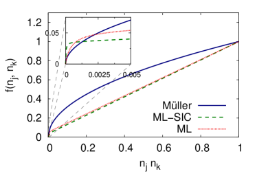
Figure 1: (Color online) Plot of the function $f(n_{j},n_{k})$ for the ML, ML-SIC and the Müller functional. The inset zooms on the particularly interesting region close to zero.

In Fig. 1 we plot the ML functionals compared to the simple Müller form. It is clear that, in order to correct for the consistent over-correlation of the Müller functional, our functionals are almost always smaller than the simple square-root (with exception of a small region close to zero). We also note that the functionals never become negative (this was true for all forms that we tried, including those with more parameters). However, the most striking fact is that the ML functionals are essentially linear except very close to zero, where their value drops quickly to zero (see inset of Fig. 1). It is also important to note that all functionals of reasonable quality that we found exhibited this kind of kink.

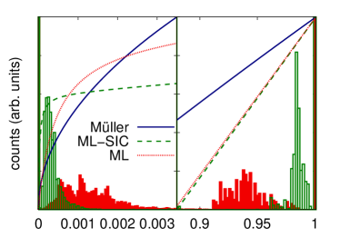
Figure 2: (Color online) Histogram with the values of $n_{j}n_{k}$ for all G2 closed-shell molecules. The values of $n_{j}n_{k}$ are obtained with the both with the ML (dashed red bars) and ML-SIC (empty green bars) functionals. Note that the left and right panels do not have the same horizontal or vertical scale.

To better understand our numerical results, we show, in Fig. 2, a histogram of the product $n_{j}n_{k}$ for all G2 closed-shell molecules, calculated both with the ML and ML-SIC functional. We can divide the product of the states in 4 different sets (we will use the nomenclature of Ref. gritsenko, ):

1. Products of weekly occupied orbitals (the large bar at zero). Note that in all cases, these weekly occupied orbitals are not pinned at zero, but instead have a very small but finite occupation.

2. Products of a weekly occupied orbital with a strongly occupied orbital. These are the products whose values lie mainly between zero and $\sim 3\times 10^{-3}$, but with a long tail that extends to $n_{j}n_{k}=0.25$ (ML) and $n_{j}n_{k}=0.15$ (ML-SIC).

3. Products of two strongly occupied orbitals. These have a tail that extends from $n_{j}n_{k}=0.83$ (ML) and $n_{j}n_{k}=0.95$ (ML-SIC) to one.

4. Products of two pinned states at one. For curiosity, we refer that both the ML and ML-SIC functionals yield exactly the same number of pinned orbitals for the molecules considered.

The ML functional lead to occupation numbers (and corresponding products $n_{j}n_{k}$) with a much broader distribution than ML-SIC. This is not surprising, as the width of the distribution can be seen as a measure of “correlation”. In the ML-SIC functional, a large contribution of the exchange-correlation energy (the self-interaction) has been explicitly subtracted, so the resulting occupation numbers will seem less correlated. We stress, however, that from the point of view of the total correlation energy both ML and ML-SIC fare equally well, even if it apparently easier to construct SIC functionals.

The analysis of the picture also makes clear a path to improve RDMFT functionals: to use different functional forms to approximate the exchange-correlation in each of the well-separated ranges corresponding to weakly-weakly, weakly-strongly, and strongly-strongly occupied states. The price to pay is a clear increase of the complexity of the functional. This is, in fact, the path already used by, for example, the BBC correctionsgritsenko .

In conclusion, in this Article we proposed a very simple empirical functional to be used within RDMFT. This functional is very precise, reaching in some respects the accuracy of more traditional quantum chemical approaches, like MP2 theory. Perhaps surprisingly, we can reach the same level of average accuracy using functionals that are explicitly self-interacted corrected or not. This fact is further analyzed by looking at the basic ingredient of the functionals: the product $n_{j}n_{k}$ between the occupation numbers of two states.

- (1) T. L. Gilbert, Phys. Rev. B12, 2111 (1975).
- (2) A. M. K. Müller, Phys. Lett. A 105, 446 (1984).
- (3) M. A. Buijse, E. J. Baerends, Mol. Phys. 100, 401 (2002); M.A. Buijse, PhD Thesis, Vrije Universiteit Amsterdam (1991).
- (4) S. Goedecker, C. J. Umrigar, Phys. Rev. Lett. 81, 866 (1998).
- (5) V. N. Staroverov and G. E. Scuseria, J. Chem. Phys. 117, 2489 (2002).
- (6) J. M. Herbert, J. E. Harriman, Chem. Phys. Lett. 382, 142 (2003).
- (7) J. Cioslowski and K. Pernal, J. Chem. Phys. 111, 3396 (1999).
- (8) G. Csányi and T. A. Arias, Phys. Rev. B 61, 7348 (2000).
- (9) N. N. Lathiotakis, N. Helbig, and E. K. U. Gross, Phys. Rev. B 75, 195120 (2007)
- (10) O. Gritsenko, K. Pernal, E. J. Baerends, J. Chem. Phys., 122, 204102 (2005).
- (11) M. Piris, Int. J. Quant. Chem. 106, 1093 (2006).
- (12) N. N. Lathiotakis and M. A. L. Marques, submitted to J. Chem. Phys.
- (13) K. Pernal, J. Cioslowski, Chem. Phys. Lett., 412, 71 (2005).
- (14) P. Leiva and M. Piris, J. Chem. Phys., 123, 214102 (2005).
- (15) P. Leiva, M. Piris, J. Mol. Struct.-Theochem., 770, 45 (2006).
- (16) P. Leiva, M. Piris, Int. J. Quant. Chem., 107, 1 (2007).
- (17) N. N. Lathiotakis, N. Helbig, and E. K. U. Gross, Phys. Rev. B 75, 195120 (2007).
- (18) K. Pernal, E. J. Baerends, J. Chem. Phys., 124, 014102 (2006).
- (19) G. E. Scuseria and V. N. Staroverov, in Theory and Applications of Computational Chemistry: The First Forty Years, ed. by C. E. Dykstra, G. Frenking, K. S. Kim, and G. E. Scuseria, p. 669–724 (Elsevier, Amsterdam, 2005).
- (20) See, e.g., D. J. Tozer, N. C. Handy, J. Chem. Phys. 108 2545 (1998); F. A. Hamprecht, A. J. Cohen, D. J. Tozer, N. C. Handy, J. Chem. Phys. 109 6264 (1998); G. K.-L. Chan, N. C. Handy, J. Chem. Phys. 112 5639 (2000); P. J. Wilson, T. J. Bradley, D. J. Tozer, J. Chem. Phys. 115 9233 (2001).
- (21) L. A. Curtiss, K. Raghavachari, P. C. Redfern, and J. A. Pople, J. of Chem. Phys. 106, 1063 (1997); L. A. Curtiss, P. C. Redfern, K. Raghavachari, and J. A. Pople, J. of Chem. Phys., 109, 42 (1998).
- (22) G. Csányi, S. Goedecker, T. A. Arias, Phys. Rev. A65 032510 (2002).