Evolution of arbitrary spin fields in the Schwarzschild-monopole spacetime

Abstract

The quasinormal modes (QNMs) and the late-time behavior of arbitrary spin fields are studied in the background of a Schwarzschild black hole with a global monopole (SBHGM). It has been shown that the real part of the QNMs for a SBHGM decreases as the symmetry breaking scale parameter $H$ increases but imaginary part increases instead. For large overtone number $n$, these QNMs become evenly spaced and the spacing for the imaginary part equals to $-i(1-H)^{3/2}/(4M)$ which is dependent of $H$ but independent of the quantum number $l$. It is surprisingly found that the late-time behavior is dominated by an inverse power-law tail $t^{-2[1+\sqrt{(s+1/2)^{2}+(l-s)(l+s+1)/(1-H)}]}$ for each $l$, and as $H\rightarrow 0$ it reduces to the Schwarzschild case $t^{-(2l+3)}$ which is independent of the spin number $s$.

The evolution of the external field perturbation around a black hole is dominated by three successive stages Frolov98 ; Kokkotas ; Nollert : the initial wave burst, the damped oscillations called QNMs and the power-law tail behavior of the waves at very late time. A well-known fact is that the QNMs have become astrophysically significant with the realistic possibility of gravitational wave detection in the near future because they are entirely fixed by the structure of the background vishe ; Chand ; Leaver ; Cardoso ; J-2 . In addition, the study of the QNMs can also help us get a deeper understandings of the loop quantum gravity Hod ; Dreyer , AdS/CFT and dS/CFT correspondences Maldacena ; Witten ; Kalyana . On the other hand, the late-time evolution of various field perturbations has important implications for two major aspects of black-hole physics: the no-hair theorem and the mass-inflation scenario Ruffini ; Misner ; Price ; Leaver-1 ; Piran-tail ; Hod-tail ; LMBurko ; J-4 ; J-5 . Thus, we will discuss the evolution of massless arbitrary spin fields around a SBHGM which is introduced by Barriola and Vilenkin Barriola , including the QNMs and late-time tails in this short note. And our purpose is to see what effects the symmetry breaking scale parameter and the spin number will have on the evolution of the external field perturbation.

In the Boyer-Lindquist coordinates $(t,r,\theta,\varphi)$, the metric for a SBHGM is Barriola ; Bertrand ; Salgado ; Yu

$$ds^{2}=\frac{\Delta_{r}}{r^{2}}dt^{2}-\frac{r^{2}}{\Delta_{r}}dr^{2}-r^{2}(1-H)(d\theta^{2}+sin^{2}\theta d\varphi^{2}),$$ (1)

where $\Delta_{r}=r^{2}-2M(1-H)^{-3/2}r$ and $H=8\pi\eta_{0}^{2}$, $M$ and $\eta_{0}$ represent the mass parameter of the black hole and the symmetry breaking scale when the monopole is formed respectively. Throughout this paper we use $G=c=1$. In this spacetime the Teukolsky’s master equations for massless arbitrary spin fields Teukolsky-1 ; Teukolsky-2 ; Teukolsky-3 ; Teukolsky-4 can be separated by using the Newman-Penrose formalism Newman . After the tedious calculation, we find that the angular equation is the same as in the Schwarzschild black hole Newman ; Teukolsky-1 ; Teukolsky-2 ; Teukolsky-3 ; Teukolsky-4 and the radial equation can be expressed as

$$\frac{d^{2}\Psi_{s}}{dr_{*}^{2}}+[\omega^{2}-V_{s}(r)]\Psi_{s}=0,$$ (2)

with

$$V_{s}(r)=is\omega r^{2}\frac{d}{dr}\left(\frac{\Delta_{r}}{r^{4}}\right)+\frac{1}{r^{4}}\left[\left(\frac{s}{2}\frac{d\Delta_{r}}{dr}\right)^{2}+\left(s+\frac{\lambda}{1-H}\right)\Delta_{r}\right]-\frac{\Delta_{r}}{r^{3}}\frac{d}{dr}\left[\Delta_{r}\frac{d}{dr}\left(\frac{1}{r}\right)\right],$$ (3)

where $dr_{*}=(r^{2}/\Delta_{r})dr$ and $\Psi_{s}=\Delta^{s/2}_{r}r^{1-2s}R_{s}$ ($R_{s}$ is the usual radial wave function Newman ; Teukolsky-1 ; Teukolsky-2 ; Teukolsky-3 ; Teukolsky-4 ), $\lambda=(l-s)(l+s+1)$ is the angular separation constant for $s=0,\ \ -1/2,\ \ -1,\ \ -3/2$ and $-2$ with the quantum number $l=|s|,|s|+1,\cdots$.

Quasinormal Modes Introducing the expansion coefficients $d_{n}$, we can give a solution to Eq. (2)

$$\Psi_{s}=r^{-\frac{s}{2}+2i\omega r_{+}}(r-r_{+})^{-\frac{s}{2}-i\omega r_{+}}e^{i\omega r}\sum_{n=0}^{\infty}d_{n}\left(\frac{r-r_{+}}{r}\right)^{n},$$ (4)

which satisfies the desired behavior at the boundary for the SBHGM Chand . Thus, the three-term continued fraction equation is written as Leaver

$$0=\beta_{0}-\frac{\alpha_{0}\gamma_{1}}{\beta_{1}-}\frac{\alpha_{1}\gamma_{2}}{\beta_{2}-}\frac{\alpha_{2}\gamma_{3}}{\beta_{3}-}\frac{\alpha_{3}\gamma_{4}}{\beta_{4}-}\cdots,$$ (5)

with

$$\alpha_{n}=n^{2}+\left[2-s-\frac{4iM\omega}{\sqrt{(1-H)^{3}}}\right]n+\left[1-s-\frac{4iM\omega}{\sqrt{(1-H)^{3}}}\right],$$

$$\beta_{n}=-2n^{2}-\left[2-\frac{16iM\omega}{\sqrt{(1-H)^{3}}}\right]n-\left[1+s-\frac{8iM\omega}{\sqrt{(1-H)^{3}}}-\frac{32M^{2}\omega^{2}}{(1-H)^{3}}+\frac{\lambda}{1-H}\right],$$

$$\gamma_{n}=n^{2}+\left[s-\frac{8iM\omega}{\sqrt{(1-H)^{3}}}\right]n-\left[\frac{4isM\omega}{\sqrt{(1-H)^{3}}}+\frac{16M^{2}\omega^{2}}{(1-H)^{3}}\right].$$ (6)

Eq. (5) has an infinite number of roots (corresponding to the QNMs), but for each overtone number $n$, the QNMs $\omega_{n}$ depend on the symmetry breaking scale parameter $H$, spin number $s$ and quantum number $l$ if we take $2M=1$.

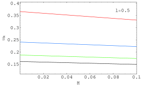
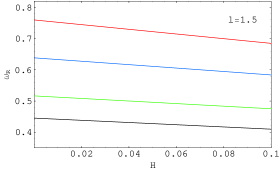
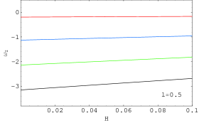
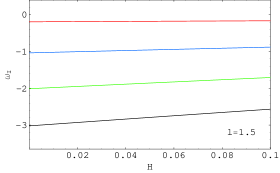
Figure 1: (Color online) Dependence of the real part $\omega_{R}$ and imaginary part $\omega_{I}$ on $H$ for the Dirac QNMs of the SBHGM. In each panel, the four lines from the top to the bottom correspond to the modes for $n=0$ (red), $n=2$ (blue), $n=4$ (green) and $n=6$ (black) respectively.

Figure 2: The spacing $\Delta\omega_{I}$ as the functions of overtone number $n$ for $l=1/2$ and $l=3/2$. These panels shows that $\Delta\omega_{I}$ is dependent of $H$ but independent of $l$ for large n.

For universality and clarity we only show some numerical results of a massless Dirac field ($s=-1/2$) in Figs. 1 and 2. After discussing the other spin fields, we point out that: (i) The QNMs of the massless arbitrary spin fields around the SBHGM depend on $H$, and the real part $\omega_{R}$ of the QNMs decreases as $H$ increases but imaginary part $\omega_{I}$ increases. (ii) The spacing for imaginary part of the QNMs for the massless arbitrary spin fields in the background of the SBHGM is

$$Im(\omega_{n+1})-Im(\omega_{n})\approx-\frac{i}{4M}(1-H)^{3/2},~{}~{}~{}~{}{\text{as}}~{}~{}~{}n\rightarrow\infty,$$ (7)

which is dependent of $H$ but independent of $l$.

Late-time Behavior Let us assume the observer and the initial data are situated far away from the black hole. Then, neglecting terms of order $0(\omega/r^{2})$ and the higher order terms, we expand the wave equation (2) as a power series in $M/r$

$$\left[\frac{d^{2}}{dr^{2}}+\omega^{2}+\frac{2is\omega+4M(1-H)^{-3/2}\omega^{2}}{r}-\frac{1}{r^{2}}\left(s+s^{2}+\frac{\lambda}{1-H}\right)\right]\xi_{s}(r,\omega)=0,$$ (8)

where $\xi_{s}=(\sqrt{\Delta_{r}}/r)\Psi_{s}$. So two basic solutions required in order to build the Green’s function can be expressed as

$$\tilde{\Psi}_{1}=Ar^{\rho+1/2}e^{i\omega r}M(1/2+\rho+s-2iM(1-H)^{-3/2}\omega,1+2\rho,-2i\omega r),$$

$$\tilde{\Psi}_{2}=Br^{\rho+1/2}e^{i\omega r}U(1/2+\rho+s-2iM(1-H)^{-3/2}\omega,1+2\rho,-2i\omega r),$$ (9)

where $\rho=[(s+1/2)^{2}+\lambda/(1-H)]^{1/2}$, $A$ and $B$ are normalization constants. $M(a,b,z)$ and $U(a,b,z)$ are the two standard solutions to the confluent hypergeometric equation Abramowitz . The function $U(a,b,z)$ is a many-valued function, i.e., there will be a cut in $\tilde{\Psi}_{2}$.

It has been argued that the late-time tail is associated with the existence of a branch cut (in $\tilde{\Psi}_{2}$) Leaver-1 ; Piran-tail ; Hod-tail . The branch cut contribution to the Green’s function can be written as

$$G^{c}_{s}(r_{*},r^{\prime}_{*};t)=\frac{1}{2\pi}\int_{0}^{-i\infty}\tilde{\Psi}_{1}(r^{\prime}_{*},\omega)\left[\frac{\tilde{\Psi}_{2}(r_{*},\omega e^{2\pi i})}{W_{s}(\omega e^{2\pi i})}-\frac{\tilde{\Psi}_{2}(r_{*},\omega)}{W_{s}(\omega)}\right]e^{-i\omega t}d\omega,$$ (10)

where $W_{s}(\omega)=\tilde{\Psi}_{1}\tilde{\Psi}_{2,r_{*}}-\tilde{\Psi}_{2}\tilde{\Psi}_{1,r_{*}}$ is the Wronskian. Since we are only interested in the leading-order behavior at very late times, we can assume that $\omega r^{\prime}_{*}<\omega r_{*}<1$. Thus, with the help of Ref. Abramowitz , we obtain the late-time behavior at timelike infinity

$$G^{c}_{s}(r_{*},r^{\prime}_{*};t)=\Upsilon(r_{*},r^{\prime}_{*})~{}t^{-2(\rho+1)}=\Upsilon(r_{*},r^{\prime}_{*})~{}t^{-2[1+\sqrt{(s+1/2)^{2}+(l-s)(l+s+1)/(1-H)}]},$$ (11)

where $\Upsilon(r_{*},r^{\prime}_{*})$ is the integral constant. To our great surprise, this late-time behavior depends on the spin number $s$, which is never found in the previous works. Taking $H=0$, we get the late-time tails of the massless arbitrary spin fields for the Schwarzschild black hole at timelike infinity, i.e., $t^{-(2l+3)}$ which is independent of the spin number $s$. This result agrees with the Hod’s analytical work for the massless arbitrary spin fields on Kerr spacetimes Hod-tail .

Summarizing, the QNMs of massless arbitrary spin fields in the background of the SBHGM depend on the symmetry breaking scale parameter $H$, and the real part of the QNMs decreases as $H$ increases but imaginary part increases instead. For large overtone number $n$, these QNMs become evenly spaced and the spacing for the imaginary part equals to $-i(1-H)^{3/2}/(4M)$ which is dependent of $H$ but independent of the quantum number $l$. The most interesting outcome of our study is that an inverse power-law tail $t^{-2[1+\sqrt{(s+1/2)^{2}+(l-s)(l+s+1)/(1-H)}]}$ which depends on $H$ and the spin number $s$ will dominate the late-time behavior, which is shown that the SBHGM is quite different topologically from a normal black hole due to the presence of a global monopole.

- (1) Frolov V P and Novikov I D 1998 Black hole physics: basic concepts and new developments (Dordrecht: Kluwer Academic)
- (2) Kokkotas K D and Schmidt B G 1999 Living Rev. Rel. 2 2
- (3) Nollert H P 1999 Class. and Quant. Grav. 16 R159
- (4) Vishveshwara C V 1970 Nature (London) 227 936
- (5) Chandrasekhar S and Detweller S 1975 Proc. R. Soc. Lond. A 344 441
- (6) Leaver E W 1985 Proc. R. Soc. Lond. A 402 285
- (7) Cardoso V and Lemos J P S 2003 Phys. Rev. D 67 084020.
- (8) Jing J L 2005 JHEP 0512 005
- (9) Hod S 1998 Phys. Rev. Lett. 81 4293
- (10) Dreyer O 2003 Phys. Rev. Lett. 90 081301
- (11) Maldacena J M 1998 Adv. Theor. Math. Phys. 2 231
- (12) Witten E 1998 Adv. Theor. Math. Phys. 2 253
- (13) Kalyana S and Sathiapalan B 1999 Mod. Phys. Lett. A 14 2635
- (14) Ruffini R and Wheeler J A 1971 Phys. Today 24 30
- (15) Misner C W, Thorne K S and Wheeler J A 1973 Gravitation (San Francisco: Freeman)
- (16) Price R H 1972 Phys. Rev. D 5 2419
- (17) Leaver E W 1986 Phys. Rev. D 34 384
- (18) Hod S and Piran T 1998 Phys. Rev. D 58 024017
- (19) Hod S 1998 Phys. Rev. D 58 104022
- (20) Burko L M and Khanna G 2004 Phys. Rev. D 70 044018
- (21) Jing J L 2004 Phys. Rev. D 70 065004
- (22) Jing J L 2005 Phys. Rev. D 72 027501
- (23) Barriola M and Vilenkin A 1989 Phys. Rev. Lett. 63 341
- (24) Bertrand B, Brihaye Y and Hartmann B 2003 Class. and Quant. Grav. 20 4495
- (25) Salgado M 2003 Class. and Quant. Grav. 20 4551
- (26) Yu H 2002 Phys. Rev. D 65 087502
- (27) Teukolsky S A 1972 Phys. Rev. Lett. 29 1114
- (28) Teukolsky S A 1973 Astrophys. J. 185 635
- (29) Press W H and Teukolsky S A 1973 Astrophys. J. 185 649
- (30) Teukolsky S A and Press W H 1974 Astrophys. J. 193 443
- (31) Newman E and Penrose R 1962 J. Math. Phys. (N. Y.) 3 566
- (32) Abramowitz M and Stegun I A 1970 Handbook of Mathematical Functions (New York: Dover)