Abstract

In the framework of boundary conformal field theory we consider a flat unstable D$p$-brane in the presence of a large constant electromagnetic field. Specifically, we study the case that the electromagnetic field satisfy the following three conditions: (i) a constant electric field is turned on along the $x^{1}$ direction ($E_{1}\neq 0$); (ii) the determinant of the matrix $(\eta+F)$ is negative so that it lies in the physical region ($-\det(\eta+F)>0$); (iii) the 11-component of its cofactor is positive to the large electromagnetic field. In this case, we identify exactly marginal deformations depending on the spatial coordinate $x^{1}$. They correspond to tachyon profiles of hyperbolic sine, exponential, and hyperbolic cosine types. Boundary states are constructed for these deformations by utilizing T-duality approach and also by directly solving the overlap conditions in BCFT. The exponential type deformation gives a tensionless half brane connecting the perturbative string vacuum and one of the true tachyon vacua, while the others have negative tensions. This is in agreement with the results obtained in other approaches.

1 Introduction

Type IIA (IIB) string theory supports even-dimensional (odd-dimensional) stable BPS D-branes and odd-dimensional (even-dimensional) unstable nonBPS D-branes [1]. The physics of unstable D-branes involves various nonperturbative aspects of string theory. Specifically, two representative examples are the tachyon solitons interpreted as lower-dimensional D-branes [2, 3] and the rolling tachyon describing homogeneous real-time decay process of the D-brane [4, 5].

The instability of a nonBPS D$p$-brane in superstring theory or a D$p$-brane in bosonic string theory results in the appearance of a tachyonic degree. In the context of boundary conformal field theory (BCFT), the tachyon vertex operator with a single spatial dependence which represents the exactly marginal deformation is given by a sinusoidal function with a single multiplicative parameter. When the parameter has the value 1/2, the deformation is interpreted as an array of D$(p-1)$-branes in bosonic string theory or as a periodic array of a pair of a D$(p-1)$-brane and a $\bar{\rm D}(p-1)$-brane in superstring theory [2, 3, 6]. The homogeneous rolling tachyon in BCFT is described by introducing a marginal deformation corresponding to the tachyon profiles of hyperbolic sine, exponential, or hyperbolic cosine type. The physical quantities like the energy-momentum tensor suggest real-time decay of an unstable D-brane when the tachyon is displaced from the maximum of the tachyon potential and rolls down towards its minimum.

Both homogeneous rolling tachyons and lower-dimensional D-branes from an unstable D-brane have also been studied in the context of effective field theories (EFTs) such as Dirac-Born-Infeld (DBI) type EFT [7, 8, 9, 10] and boundary string field theory (BSFT) EFT [11, 12, 13]. Compared with the BCFT approach, physical quantities such as energy-momentum tensor obtained from these EFTs are qualitatively the same as, but slightly different from that in BCFT [7]–[13]. For the case of the half S-brane with the exponential type of the tachyon profile [14] which is a special case of homogeneous rolling tachyons, the energy-momentum tensor based on the formula in Ref. [5] coincides exactly with that of DBI type effective action with 1/cosh potential [15].

When the fundamental strings exist in the worldvolume of unstable D$p$-brane, they couple to the second-rank antisymmetric tensor field (or equivalently to the electromagnetic field strength tensor on the D-brane [16]) and the string current density is given by the Lorentz-covariant conjugate momentum of U(1) gauge field [17, 18, 19]. Then one may study the effect of the electromagnetic field. For rolling tachyons, the three types of deformations mentioned above are not changed by the presence of constant electric [20, 21, 22], or both electric and magnetic [23, 24] fields as far as they satisfy the physical condition, $-\det(\eta+F)>0$ where $F$ denotes the electromagnetic field strength tensor.

The situation is more interesting for the case of tachyon kinks which are identified as lower-dimensional D-branes of codimension one. The spectrum of the tachyon kink is not changed when the constant electric field is turned on with keeping $-\det(\eta+F)>0$; only the period of D$(p-1){\bar{\rm D}}(p-1)$ in the array becomes large as the electric field increases. However, when the electric field eventually reaches the critical value for which the determinant vanishes, the period becomes infinite and we obtain a single regular BPS tachyon kink with constant electric flux. It is interpreted as a thick BPS D$(p-1)$-brane in the background of fundamental string charge density. This has been checked in various languages including DBI EFT [9, 25], BCFT [26], noncommutative field theory (NCFT) [27], and BSFT [13].

In the presence of both constant electric and constant magnetic fields in an unstable D$p$-brane with $p\geq 2$, it turns out that other types of deformations are possible. This is because the 11-component of the cofactor $C^{11}$ of $(\eta+F)_{\mu\nu}$ can have either negative or positive value while keeping $-\det(\eta+F)>0$. (Here, $x^{1}$ denotes the coordinate on which the tachyon depends.) For small electromagnetic fields the cofactor $C^{11}$ is negative. In this case the species of tachyon kinks are essentially the same as those without electromagnetic field. On the other hand, when $p\geq 2$, electromagnetic fields can take large values for which $C^{11}$ becomes positive while maintaining the condition $-\det(\eta+F)>0$. In this case, three new codimension-one objects are supported, which correspond to tachyon profiles of hyperbolic sine, exponential, and hyperbolic cosine types. These objects have been obtained in aforementioned EFTs including DBI EFT [9, 25], NCFT [28], and BSFT [13]. They, however, have not yet been reproduced in the context of BCFT for type II superstring theory. The purpose of this paper is to analyze these three kinks in the context of BCFT.

In section 2, we describe new tachyon vertices of hyperbolic sine, exponential, and hyperbolic cosine types with the dependence on a single spatial coordinate, and show that they give marginal deformations in the context of BCFT. In addition, these tachyon profiles are obtained as static solutions of the linearized tachyon equation in the background of a nontrivial open string metric and a noncommutativity parameter of open string field theory (OSFT). In section 3 we construct the boundary states corresponding to the marginal deformations given in section 2. We utilize Lorentz transformation and T-duality in subsection 3.1 while the overlap condition is directly solved in subsection 3.2 to construct the boundary states. In section 4 we read the corresponding physical quantities, specifically the energy-momentum tensor $T_{\mu\nu}$ and the fundamental string current density $\Pi_{\mu\nu}$. For the case of hyperbolic sine and hyperbolic cosine types of tachyon profiles, they are slightly different from those in EFTs as expected [9, 25, 28], but, for the exponential type, they coincide exactly with the results of EFTs. They are interpreted as negative tension branes for hyperbolic sine and cosine profiles and tensionless half brane for exponential profile in the huge constant background of positive energy density. We conclude in section 5. In the appendix, we give an alternative derivation of the energy-momentum tensor for the exponential type deformation by calculating the partition function of the worldsheet action following Ref. [29].

2 New Tachyon Vertices as Exactly Marginal Deformations

In this section we show that there exist three new tachyon vertices as marginal deformations in the presence of the constant electromagnetic field. They are hyperbolic sine, hyperbolic cosine, and exponential types which depend on a single spatial coordinate. We shall show this first in the scheme of BCFT and then in the context of linearized OSFT.

In the BCFT description of bosonic string theory, the worldsheet action of a D$p$-brane in the presence of a background U(1) gauge field $A_{\mu}$ is given by

$$S_{\rm BCFT}=\frac{1}{2\pi}\int_{\Sigma}d^{2}w\,\partial X^{\mu}\bar{\partial}X_{\mu}-\frac{i}{2\pi}\int_{\partial\Sigma}dt\,A_{\mu}(X)\partial_{t}X^{\mu},$$ (2.1)

where $\Sigma$ denotes the worldsheet and $t$ parametrizes the boundary of the worldsheet. It satisfies the boundary condition

$$\left(\partial_{n}X^{\mu}+iF^{\mu}{}_{\nu}\partial_{t}X^{\nu}\right)\mid_{\partial\Sigma}=0,$$ (2.2)

where $\partial_{n}$ and $\partial_{t}$ denote respectively the normal and tangential derivatives at the boundary $\partial\Sigma$. The dynamics of an unstable D$p$-brane is described by introducing a conformally invariant boundary interaction to the worldsheet action,

$$S_{T}=\int_{\partial\Sigma}dt\,T(X).$$ (2.3)

When there is no background gauge field ($A_{\mu}=0$), it is well-known that for any spatial direction $X$ the operator

$$T(X)=\lambda\cos X$$ (2.4)

is exactly marginal and has been used to describe lower-dimensional D-branes [2, 3]. The relevant boundary state is given by [30, 31, 32]

$$|\mathcal{B}\rangle_{X}=\sum_{j=0,1/2,1,\ldots}\sum_{m=-j}^{j}D_{m,-m}^{j}(R)|j;m,m\rangle\rangle,$$ (2.5)

where $R$ is the SU(2) rotation matrix

$$R=\begin{pmatrix}\cos\pi\lambda&i\sin\pi\lambda\\ i\sin\pi\lambda&\cos\pi\lambda\end{pmatrix},$$ (2.6)

$D_{m,-m}^{j}(R)$ is the spin $j$ representation matrix of $R$ in the $J_{z}$ eigenbasis, and $|j;m,m\rangle\rangle$ is the Virasoro-Ishibashi state [33] built over the primary state $|j;m,m\rangle=|j,m\rangle\overline{|j,m\rangle}$.

The temporal version of (2.4)

$$T(X^{0})=\lambda\cosh X^{0}$$ (2.7)

describes the dynamics of the rolling tachyon [4, 5]. For example the relevant boundary state for a D$p$-brane with the deformation (2.7) is given by

$$|\mathcal{B}\rangle=|\mathcal{B}\rangle_{X^{0}}\otimes_{\mu=1}^{p}|N\rangle_{X^{\mu}}\otimes_{i=p+1}^{25}|D\rangle_{X^{i}}\otimes|\text{ghost}\rangle,$$ (2.8)

where

$$|N\rangle_{X^{\mu}} =\exp\left[-\sum_{n=1}^{\infty}\frac{1}{n}\alpha_{-n}^{\mu}\bar{\alpha}_{-n}^{\mu}\right]|0\rangle,$$

$$|D\rangle_{X^{i}} =\exp\left[\sum_{n=1}^{\infty}\frac{1}{n}\alpha_{-n}^{i}\bar{\alpha}_{-n}^{i}\right]|0\rangle,$$

$$|\text{ghost}\rangle =\exp\left[-\sum_{n=1}^{\infty}(\bar{b}_{-n}c_{-n}+b_{-n}\bar{c}_{-n})\right](c_{0}+\bar{c}_{0})c_{1}\bar{c}_{1}|0\rangle,$$ (2.9)

and $|{\cal B}\rangle_{X^{0}}$ is the boundary state (2.5) in the Wick-rotated variable $X\to-iX^{0}$.

In the presence of a constant background electric field the operator (2.7) is modified by a Lorentz factor [20],

$$T(X^{0})=\lambda\cosh(\sqrt{1-E^{2}}\,X^{0}),$$ (2.10)

where $E$ is the magnitude of the electric field. Rolling tachyons have further been generalized to the case that both electric and magnetic fields are turned on [23, 24].

In this section we would like to discuss the exactly marginal deformation $S_{T}$ (2.3) in the background of a general constant electromagnetic field for which we take the symmetric gauge,

$$A_{\mu}=-\frac{1}{2}F_{\mu\nu}X^{\nu}.$$ (2.11)

As usual [4], we first consider the Wick-rotated theory obtained by the replacement $X^{0}\rightarrow iX^{0}$ and make the inverse Wick-rotation back to the Minkowski time later.

Under the deformed boundary condition (2.2), the correlation function on the upper-half plane is obtained as [34],

$$\langle X^{\mu}(w)X^{\nu}(w^{\prime})\rangle= -\delta^{\mu\nu}\ln\mid w-w^{\prime}\mid+\delta^{\mu\nu}\ln\mid w-\bar{w}^{\prime}\mid$$

$$-\bar{G}^{\mu\nu}\ln\mid w-\bar{w}^{\prime}\mid^{2}-\bar{\theta}^{\mu\nu}\ln\left(\frac{w-\bar{w}^{\prime}}{\bar{w}-w^{\prime}}\right).$$ (2.12)

Here $\bar{G}_{\mu\nu}$ and $\bar{\theta}^{\mu\nu}$ are the Wick-rotated version of the open string metric $G^{\mu\nu}$ and the noncommutativity parameter $\theta^{\mu\nu}$ given as

$$G^{\mu\nu}=\left(\frac{1}{\eta+F}\right)^{\mu\nu}_{{\rm S}}=\frac{C^{\nu\mu}_{{\rm S}}}{{\cal Y}_{p}},\qquad\theta^{\mu\nu}=\left(\frac{1}{\eta+F}\right)^{\mu\nu}_{{\rm A}}=\frac{C^{\nu\mu}_{{\rm A}}}{{\cal Y}_{p}},$$ (2.13)

where $C_{{\rm S}}^{\mu\nu}$ and $C_{{\rm A}}^{\mu\nu}$ are respectively the symmetric and antisymmetric parts of $C^{\mu\nu}$, the cofactor matrix of $(\eta+F)_{\mu\nu}$, and ${\cal Y}_{p}\equiv\det(\eta+F)$. When $w^{\prime}$ is on the boundary, (2.12) reduces to

$$X^{\mu}(w)X^{\nu}(t)\sim-\bar{G}^{\mu\nu}\ln|w-t|^{2}-\bar{\theta}^{\mu\nu}\ln\left(\frac{w-t}{\bar{w}-t}\right),$$ (2.14)

where $t$ represents the boundary. Since the OPE of the energy-momentum tensor $T=-\partial X^{\mu}\partial X_{\mu}$ with the tachyon boundary vertex operator $e^{ik\cdot X(t)}$ is

$$T(w)e^{ik\cdot X(t)}\sim\frac{\bar{G}^{\mu\nu}k_{\mu}k_{\nu}}{(w-t)^{2}}\,e^{ik\cdot X(t)}+\frac{1}{w-t}\,\partial_{t}(e^{ik\cdot X(t)}),$$ (2.15)

this operator becomes marginal when

$$\bar{G}^{\mu\nu}k_{\mu}k_{\nu}=1.$$ (2.16)

In this paper we are interested in the operators which depend on a single spatial coordinate. For definiteness we take $k_{\mu}\propto\delta_{\mu 1}$ and denote $X=X^{1}$ for the sake of simplicity. In this case (2.16) reduces to $k_{1}^{2}=1/{\bar{G}^{11}}$. Then the boundary operator is not only marginal but actually exactly marginal [32] since the second term containing the noncommutative parameter in (2.14) plays no role. After the inverse Wick rotation, the marginality condition then leads to

$$k_{1}^{2}=\frac{1}{G^{11}}=\frac{{\cal Y}_{p}}{C^{11}}.$$ (2.17)

As an example, let us consider an unstable D2-brane ($p=2$) with a constant electromagnetic field $F_{0i}=E_{i}$ (${\bf E}^{2}=E_{i}^{2}$) and $F_{12}=B$. In this case, ${\cal Y}_{2}=-(1-{\bf E}^{2}+B^{2})$ and $C^{11}=-1+E_{2}^{2}$ so that the marginality condition (2.17) becomes

$$k_{1}^{2}=\frac{-(1-{\bf E}^{2}+B^{2})}{-(1-E_{2}^{2})}.$$ (2.18)

Before discussing the physical meaning of these marginal deformations, we extend our analysis to the superstring case with worldsheet fermions, $\psi^{\mu}$ and $\bar{\psi}^{\mu}$, $\mu=0,1,\ldots,9$. The worldsheet action with a constant electromagnetic field is

$$S_{{\rm w}}=\frac{1}{2\pi}\int_{\Sigma}d^{2}z\left(\partial X^{\mu}{\bar{\partial}}X_{\mu}+\frac{1}{2}\psi^{\mu}{\bar{\partial}}\psi_{\mu}+\frac{1}{2}\bar{\psi}^{\mu}\partial\bar{\psi}_{\mu}\right)-\frac{i}{2\pi}\int_{\partial\Sigma}dt\left(A_{\mu}\partial_{t}X^{\mu}-F_{\mu\nu}\Psi^{\mu}\Psi^{\nu}\right),$$ (2.19)

where the fermions in the boundary interaction always appear as the following combination,

$$\Psi^{\mu}=\frac{1}{2}(\psi^{\mu}+\bar{\psi}^{\mu}).$$ (2.20)

In addition to the boundary condition for bosonic degrees (2.2), we impose that for fermionic degrees,

$$(\eta_{\mu\nu}-F_{\mu\nu})\psi^{\nu}\big{|}_{\partial\Sigma}=\epsilon(\eta_{\mu\nu}+F_{\mu\nu}){\bar{\psi}}^{\nu}\big{|}_{\partial\Sigma}\,,$$ (2.21)

where $\epsilon=\pm$. Without the background gauge field, the following operator which represents the tachyon field $T(x)=\sqrt{2}\lambda\cos(x/\sqrt{2})$,

$$-i\sqrt{2}\lambda\psi\sin(X/\sqrt{2})\otimes\sigma_{1}$$ (2.22)

is known to be exactly marginal. Here we have assigned the Chan-Paton factor $\sigma_{1}$ and the relevant boundary state is

$$|\mathcal{B},\epsilon\rangle_{X,\psi}=\sum_{j=0,1,\ldots}\sum_{m=-j}^{j}D_{m,-m}^{j}(R)|j;m,m,\epsilon\rangle\rangle,$$ (2.23)

where $|j;m,m,\epsilon\rangle\rangle$ is the super-Virasoro-Ishibashi state built over the primary state $|j;m,m,\epsilon\rangle$ and $\epsilon=\pm$ correspond to the two different boundary conditions for the fermions in (2.21).

Taking the inverse Wick rotation, the deformation (2.22) describes the rolling tachyon in superstring theory [5]. The boundary state for the D$p$-brane with this interaction is given by

$$|\mathcal{B}\rangle=|\mathcal{B},+\rangle-|\mathcal{B},-\rangle,$$ (2.24)

where

$$|\mathcal{B},\epsilon\rangle=|\mathcal{B},\epsilon\rangle_{X^{0},\psi^{0}}\otimes_{\mu=1}^{p}|N,\epsilon\rangle_{X^{\mu},\psi^{\mu}}\otimes_{i=p+1}^{9}|D,\epsilon\rangle_{X^{i},\psi^{i}}\otimes|\text{ghost},\epsilon\rangle.$$ (2.25)

Here $|\mathcal{B},\epsilon\rangle_{X^{0},\psi^{0}}$ is the boundary state (2.23) in the Wick-rotated variables $X=-iX^{0}$, $\psi=-i\psi^{0}$, and $\bar{\psi}=-i\bar{\psi}^{0}$, and the spatial and ghost parts are usual ones, which are respectively given by

$$|N,\epsilon\rangle_{X^{\mu},\psi^{\mu}} =\exp\left[-\sum_{n=1}^{\infty}\frac{1}{n}\alpha_{-n}^{\mu}\bar{\alpha}_{-n}^{\mu}-i\epsilon\sum_{r=1/2}^{\infty}\psi_{-r}^{\mu}\bar{\psi}_{-r}^{\mu}\right]|0\rangle,$$

$$|D,\epsilon\rangle_{X^{i},\psi^{i}} =\exp\left[\sum_{n=1}^{\infty}\frac{1}{n}\alpha_{-n}^{i}\bar{\alpha}_{-n}^{i}+i\epsilon\sum_{r=1/2}^{\infty}\psi_{-r}^{i}\bar{\psi}_{-r}^{i}\right]|0\rangle,$$

$$|\text{ghost},\epsilon\rangle =\exp\left[-\sum_{n=1}^{\infty}(\bar{b}_{-n}c_{-n}+b_{-n}\bar{c}_{-n})+i\epsilon\sum_{r=1/2}^{\infty}(\beta_{-r}\bar{\gamma}_{-r}-\bar{\beta}_{-r}\gamma_{-r})\right]|\Omega\rangle,$$

$$|\Omega\rangle =(c_{0}+\bar{c}_{0})c_{1}\bar{c}_{1}e^{-\phi(0)-\bar{\phi}(0)}|0\rangle.$$ (2.26)

Now we consider the marginality condition of the tachyon vertex operator with momentum $k$ in the presence of the constant electromagnetic field. The vertex operator in the zero-picture is given by

$$-\sqrt{2}k\cdot\Psi e^{ik\cdot X(t)}.$$ (2.27)

Since the fermion $\Psi$ has conformal weight $1/2$, the marginality condition becomes

$$G^{\mu\nu}k_{\mu}k_{\nu}=\frac{1}{2}.$$ (2.28)

If we consider the operators which depend only on $X^{1}$, this condition reduces to

$$k_{1}^{2}=\frac{1}{2G^{11}}=\frac{{\cal Y}_{p}}{2C^{11}}.$$ (2.29)

In the absence of the electromagnetic field, $C^{11}={\cal Y}_{p}=-1$ and hence $k_{1}^{2}=1$ and $1/2$, respectively, for the bosonic and superstring case, as it should be. As the electromagnetic field is turned on $C^{11}$ and ${\cal Y}_{p}$ change and so does $k_{1}^{2}$. It has a positive value as long as both ${\cal Y}_{p}$ and $C^{11}$ are negative. In (2.18), this is the case when $E_{2}^{2}<1$ with an appropriate $B$ to keep ${\cal Y}_{2}$ negative. The marginal tachyon vertex operator is then of the trigonometric type: $T(X)=\lambda\cos\left(k_{1}X\right)$ or $\lambda\sin\left(k_{1}X\right)$. If we examine the corresponding energy-momentum tensor and the R-R coupling, the resulting configuration with $\lambda=1/2$ for pure tachyon case (${\cal Y}_{p}=C^{11}=-1$) is interpreted as an array of D-branes for the bosonic case or an array of D($p-1$)$\bar{\rm D}(p-1)$ for superstrings [2, 3]. It was also discussed in the presence of electric field (${\cal Y}_{1}=-1+E^{2},$ $C^{11}=-1$) [26, 9, 25].

On the other hand, if the electromagnetic field is sufficiently strong, ${\cal Y}_{p}$ and/or $C^{11}$ can be flipped to be positive. From the physical ground, the determinant ${\cal Y}_{p}$ should be negative and then the question is whether $C^{11}$ can become positive while keeping ${\cal Y}_{p}$ negative. It turns out that this is possible when $p\geq 2$ as we see in (2.18). Note that when $E_{2}^{2}>1$, $C^{11}$ becomes positive while ${\cal Y}_{p}$ remains negative as long as the magnetic field $B$ is sufficiently strong.

Then the tachyon profile becomes of the hyperbolic type $T(X)=e^{\pm\kappa X}$ where

$$\kappa\equiv ik_{1}\,=\left\{\begin{array}[]{ll}\sqrt{\frac{-{\cal Y}_{p}}{C^{11}}}&\mbox{for}\,\,\mbox{bosonic}\,\,\mbox{string},\\ \sqrt{\frac{-{\cal Y}_{p}}{2C^{11}}}&\mbox{for}\,\,\mbox{superstrings}.\\ \end{array}\right.$$ (2.30)

This is in contrast with the rolling tachyons in which $k_{0}^{2}={\cal Y}_{p}/C^{00}$ is always negative. Actually $C^{00}$ is positive irrespective of the values of constant electromagnetic field and the dimension $p$ of D-brane. Therefore turning on the electromagnetic field does not give rise to a new type of deformation for the case of rolling tachyons.

Without loss of the generality, the tachyon profile may be classified into the following three cases depending on the asymptotic behaviors,

$$\frac{T(X)}{\alpha}=\begin{cases}\mbox{(i)}&\lambda\sinh(\kappa X)\,,\\ \mbox{(ii)}&\lambda\exp(\pm\kappa X)\,,\\ \mbox{(iii)}&\lambda\cosh(\kappa X)\,,\end{cases}$$ (2.31)

where $\alpha=1$ for bosonic string and $\alpha=\sqrt{2}$ for superstrings. Note that the coordinate $X$ is a spatial direction along the D-brane. Nevertheless the form of the operator looks like that of rolling tachyons thanks to the strong electromagnetic field. This deformation is however entirely physical and can be obtained through a chain of maps involving T-duality, Lorentz boost, and rotation [23] as discussed in subsection 3.1 where the corresponding boundary state is constructed.

One comment is in order. For bosonic string, the boundary term is the same as the tachyon profile (2.31). For superstrings, tachyon vertex operators corresponding to (2.31) in the $-1$-picture are of the form $e^{-\phi}T(X)$. Since the picture number of the boundary term should be zero, each boundary term corresponding to the tachyon vertex (2.31) is obtained by picture-changing from $-1$ to 0-picture,

$$\begin{cases}\mbox{(i)}&2i\lambda\kappa\Psi\cosh(\kappa X)\otimes\sigma_{1}\,,\\ \mbox{(ii)}&\pm 2i\lambda\kappa\Psi\exp(\pm\kappa X)\otimes\sigma_{1}\,,\\ \mbox{(iii)}&2i\lambda\kappa\Psi\sinh(\kappa X)\otimes\sigma_{1}\,,\end{cases}$$ (2.32)

where the Chan-Paton factor $\sigma_{1}$ is necessary to describe GSO-odd states.

The tachyon profiles (2.31) can also be obtained in the framework of OSFT. Let us consider the linearized equations of motion in OSFT ignoring the interaction among various fields except the coupling to constant electromagnetic field. Near the perturbative string vacuum, the tachyonic degree due to the instability of an unstable D-brane can be described by a real scalar field $T$ and its action in the presence of the constant electromagnetic field is expressed in terms of an open string metric $G^{\mu\nu}$ and a noncommutativity parameter $\theta^{\mu\nu}$ in (2.13),

$$S_{{\rm L}}=\int d^{p+1}x\sqrt{-G}\left(-\frac{G^{\mu\nu}}{2}\partial_{\mu}T\ast\partial_{\nu}T-\frac{m^{2}}{2}T\ast T\right),$$ (2.33)

where $G=\det G_{\mu\nu}$ and $\ast$ denotes star product between the tachyon fields. $m^{2}<0$ is the square of the tachyon mass which is equal to $-1$ for bosonic string theory and $-1/2$ for superstring theory in our convention. Since the background electromagnetic field is constant on the flat D-brane with the metric $\eta_{\mu\nu}$, both $G^{\mu\nu}$ and $\theta^{\mu\nu}$ in (2.13) are also constant. In addition, every star product in the action (2.33), quadratic in the tachyon, can be replaced by an ordinary product and the equation of motion for the tachyon field becomes

$$G^{\mu\nu}\partial_{\mu}\partial_{\nu}T=m^{2}T.$$ (2.34)

For the static kink configurations of codimension-one objects, we assume $T=T(x),(x=x^{1})$, and then the equation of motion (2.34) reduces to

$$-C^{11}T^{\prime\prime}=-{\cal Y}_{p}m^{2}T,$$ (2.35)

where the prime ^′ denotes differentiation of $x$. To keep the role of spacetime variables, the determinant ${\cal Y}_{p}$ should be nonpositive and, to obtain nontrivial configurations, $C^{11}$ should be nonvanishing.

As discussed in the previous subsection, the types of the solution of (2.35) depend on $k_{1}^{2}={\cal Y}_{p}/C^{11}|m^{2}|$. When $C^{11}$ is positive, the solution is given by (2.31). In the absence of the electromagnetic field, $-C^{11}=1$ and although the obtained tachyon configurations (2.31) are static solutions of the linearized tachyon equation with the coupling of constant electromagnetic field, the linear tachyon system is obtained through a consistent truncation of full open string field equations restricting the fields to a universal subspace and then the obtained solutions (2.31) are expected to be solutions of full open string equations [4, 5, 20].

3 Construction of Boundary States for New Codimension-one Objects

In this section we construct the boundary state for the hyperbolic type of marginal deformation (2.31) along a spatial direction in the presence of a strong constant electromagnetic field. For definiteness we concentrate on a D25-brane in bosonic string theory. Then the case of superstring theory will briefly be discussed. The generalization to lower-dimensional D-branes is straightforward.

3.1 T-duality approach

In the following we shall construct the corresponding boundary state through a chain of transformations starting from a well-established configuration which turns out to be the rolling tachyon in the presence of the constant electric field. The order of the transformations is as follows. We begin with a D25-brane where a constant electric field is turned on along the $y^{1}$-direction and all the other excitations are set to zero except the rolling tachyon. We compactify the $y^{2}$-direction on a circle and T-dualize the D25-brane to a D24-brane. Then we boost it twice: first along the $y^{1}$-direction and then along the $y^{2}$-direction. Subsequently we rotate it in the $y^{1}y^{2}$-plane. Finally we T-dualize it back along the $y^{2}$-direction. The resulting configuration will be a D25-brane with the deformation given in (2.31).

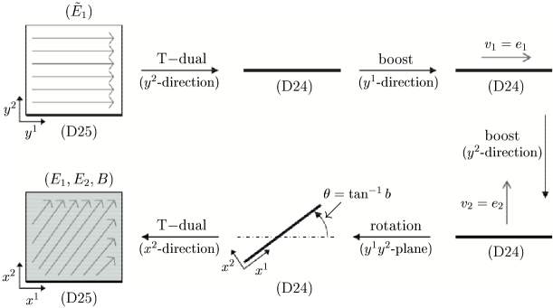
Figure 1: The arrows in D25-branes represent electric fields. The gray background in the second D25-brane represents a nonvanishing magnetic field.

Let us first consider a flat D25-brane ($p=25$) with rolling tachyon in a constant electric field. We denote the worldsheet fields of the brane by $Y^{\mu}$ and assume that the constant electric field denoted by $\tilde{E}_{1}$ is along the $y^{1}$-direction. The rolling tachyon is then described by the exactly marginal boundary operator [20]

$$\lambda\int dt\cosh\left(\sqrt{1-\tilde{E}_{1}^{2}}\,Y^{0}(t)\right).$$ (3.1)

We compactify the $y^{2}$-direction on a circle of radius $R$ and wrap the D25-brane on it.

Under the T-dualization of the $y^{2}$-direction, the right-moving part of $Y^{2}$ changes its sign while the other fields remain unchanged,

$$\mbox{T dual:}\quad Y_{R}^{2}(\bar{z})\longrightarrow-Y_{R}^{2}(\bar{z}).$$ (3.2)

The D25-brane is then turned into an array of D24-branes on the dual circle. Taking the decompactification limit $R\rightarrow\infty$ we get a localized D24-brane with a constant electric field $\tilde{E}_{1}$ turned on along the $y^{1}$-direction. The $Y^{2}$ part of the boundary state is given by the Dirichlet state,

$$|D\rangle_{Y^{2}}=\exp\left(\sum_{n=1}^{\infty}\frac{1}{n}\beta_{-n}^{2}\bar{\beta}_{-n}^{2}\right)\delta({\hat{y}^{2}})|0\rangle\,,$$ (3.3)

where $\beta_{n}^{\mu}$ and $\bar{\beta}_{n}^{\mu}$ denote the oscillators of $Y^{\mu}$.

Next, we boost the D24-brane along the $y^{1}$-direction with a velocity $e_{1}$ which is followed by another boost along the $y^{2}$-direction with a velocity $e_{2}$. Then we perform a rotation in the $y^{1}y^{2}$-plane by an angle $\tan^{-1}b$. Then $Y^{0},Y^{1},Y^{2}$ are mapped as

$$\begin{pmatrix}Y^{0}\\ Y^{1}\\ Y^{2}\end{pmatrix}\longrightarrow\begin{pmatrix}X^{0}\\ X^{1}\\ X^{2}\end{pmatrix}=\Omega\Lambda_{2}\Lambda_{1}\begin{pmatrix}Y^{0}\\ Y^{1}\\ Y^{2}\end{pmatrix}.$$ (3.4)

Here the boost transformations, $\Lambda_{1}$ and $\Lambda_{2}$, and the rotation $\Omega$ are

$$\Lambda_{1} =\begin{pmatrix}\gamma_{1}&\gamma_{1}e_{1}&0\\ \gamma_{1}e_{1}&\gamma_{1}&0\\ 0&0&1\end{pmatrix}, \gamma_{1} =\frac{1}{\sqrt{1-e_{1}^{2}}}, e_{1}^{2}<1,$$

$$\Lambda_{2} =\begin{pmatrix}\gamma_{2}&0&\gamma_{2}e_{2}\\ 0&1&0\\ \gamma_{2}e_{2}&0&\gamma_{2}\end{pmatrix}, \gamma_{2} =\frac{1}{\sqrt{1-e_{2}^{2}}}, e_{2}^{2}<1,$$

$$\Omega =\begin{pmatrix}1&0&0\\ 0&\tilde{\gamma}&-\tilde{\gamma}b\\ 0&\tilde{\gamma}b&\tilde{\gamma}\end{pmatrix}, \tilde{\gamma} =\frac{1}{\sqrt{1+b^{2}}}, 0<b^{2}<\infty,$$ (3.5)

and then the resulting transformation matrix is

$$\Omega\Lambda_{2}\Lambda_{1}=\begin{pmatrix}\gamma_{1}\gamma_{2}&\gamma_{1}\gamma_{2}e_{1}&\gamma_{2}e_{2}\\ -\gamma_{1}\gamma_{2}\tilde{\gamma}e_{2}b+\gamma_{1}\tilde{\gamma}e_{1}&-\gamma_{1}\gamma_{2}\tilde{\gamma}e_{1}e_{2}b+\gamma_{1}\tilde{\gamma}&-\gamma_{2}\tilde{\gamma}b\\ \gamma_{1}\gamma_{2}\tilde{\gamma}e_{2}+\gamma_{1}\tilde{\gamma}e_{1}b&\gamma_{1}\gamma_{2}\tilde{\gamma}e_{1}e_{2}+\gamma_{1}\tilde{\gamma}b&\gamma_{2}\tilde{\gamma}\end{pmatrix}.$$ (3.6)

Now we choose the rotation parameter $b$ as

$$b=\frac{1}{\gamma_{2}e_{1}e_{2}},$$ (3.7)

so that the 11-component of $\Omega\Lambda_{2}\Lambda_{1}$ in (3.6) vanishes. The delta function $\delta({\hat{y}^{2}})$ in the boundary state (3.3) then becomes

$$\delta(\hat{y}^{2}) =\delta(-\gamma_{2}e_{2}\hat{x}^{0}-\gamma_{2}\tilde{\gamma}b\hat{x}^{1}+\gamma_{2}\tilde{\gamma}\hat{x}^{2})$$

$$=(\gamma_{2}\tilde{\gamma})^{-1}\delta(\hat{x}^{2}-\tilde{\gamma}^{-1}e_{2}\hat{x}^{0}-b\hat{x}^{1}).$$ (3.8)

From (3.6)–(3.1), we find that within the boundary state

$$\hat{y}^{0}=-e_{1}\gamma_{1}\tilde{\gamma}^{-1}\hat{x}^{1},\qquad\hat{y}^{1}=\frac{e_{2}b}{\gamma_{1}}\,\hat{x}^{0}+\frac{\gamma_{1}}{\tilde{\gamma}}\,\hat{x}^{1}.$$ (3.9)

Note that the zero mode $\hat{y}^{0}$ in the zeroth direction is transformed to $\hat{x}^{1}$ with the help of zero-mode constraint in (3.3) for the localized D24-brane.

As the last step, we compactify the $x^{2}$-direction on a circle and T-dualize back along the $x^{2}$-direction, which changes $X_{R}^{2}(\bar{z})$ to $-X_{R}^{2}(\bar{z})$. Finally we decompactify the $x^{2}$-direction. The whole transformation can then be written as

$$\begin{pmatrix}X_{L}^{0}\\ X_{L}^{1}\\ X_{L}^{2}\\ \end{pmatrix} =\Omega\Lambda_{2}\Lambda_{1}\begin{pmatrix}Y_{L}^{0}\\ Y_{L}^{1}\\ Y_{L}^{2}\\ \end{pmatrix},$$

$$\begin{pmatrix}X_{R}^{0}\\ X_{R}^{1}\\ X_{R}^{2}\\ \end{pmatrix} =\begin{pmatrix}1&0&0\\ 0&1&0\\ 0&0&-1\\ \end{pmatrix}\Omega\Lambda_{2}\Lambda_{1}\begin{pmatrix}1&0&0\\ 0&1&0\\ 0&0&-1\\ \end{pmatrix}\begin{pmatrix}Y_{R}^{0}\\ Y_{R}^{1}\\ Y_{R}^{2}\\ \end{pmatrix}=\Omega^{-1}\Lambda_{2}^{-1}\Lambda_{1}\begin{pmatrix}Y_{R}^{0}\\ Y_{R}^{1}\\ Y_{R}^{2}\\ \end{pmatrix}.$$ (3.10)

Moreover, the zero-mode part is transformed to

$$(\gamma_{2}\tilde{\gamma})^{-1}\delta(\hat{x}^{2}-\tilde{\gamma}^{-1}e_{2}\hat{x}^{0}-b\hat{x}^{1})|0\rangle\longrightarrow(\gamma_{2}\tilde{\gamma})^{-1}|0\rangle,$$ (3.11)

yielding the Born-Infeld factor $(\gamma_{2}\tilde{\gamma})^{-1}$, since only the zero-winding sector survives in the decompactification limit.

After the chain of these transformations, we get a D25-brane with constant electric and magnetic fields deformed by the tachyon field

$$\lambda\cosh\left(\sqrt{1-\tilde{E}_{1}^{2}}\,e_{1}\gamma_{1}\tilde{\gamma}^{-1}X^{1}\right),$$ (3.12)

where (3.9) has been used. The resulting electromagnetic fields $E_{1},E_{2},B$ on the D-brane are related to the boost and rotation parameters through

$$\tilde{E}_{1}=\frac{E_{1}}{\sqrt{1-E_{2}^{2}+B^{2}}},\quad e_{1}=\frac{\sqrt{1-E_{2}^{2}+B^{2}}}{E_{2}B},\quad e_{2}=\frac{E_{2}}{\sqrt{1+B^{2}}},\quad b=B.$$ (3.13)

To see this, and also as a check of our calculation, we apply the transformations (3.1) and (3.11) to the Neumann boundary state of a static D25-brane with a nonvanishing constant electric field $\tilde{E}_{1}=\tilde{F}_{01}=-\tilde{F}_{10}$. The nontrivial part is

$$|N;\tilde{E}^{1}\rangle_{Y^{0,1,2}}=N_{p}\sqrt{-{\tilde{\cal Y}}_{p}}\exp\left[-\sum_{n=1}^{\infty}\frac{1}{n}\beta_{-n}^{a}\bar{\tau}_{-n\,a}\right]|0\rangle,\qquad(a,b=0,1,2),$$ (3.14)

where $N_{p}$ is an overall constant and ${\tilde{\cal Y}}_{p}$ is [35]

$${\tilde{\cal Y}}_{p}=\det(\eta_{ab}+\tilde{F}_{ab})=-1+\tilde{E}_{1}^{2}.$$ (3.15)

The oscillators $\bar{\tau}_{-n}$’s are defined as

$$\bar{\tau}=\tilde{M}\bar{\beta}\equiv\eta\left(\frac{\eta-\tilde{F}}{\eta+\tilde{F}}\right)\bar{\beta}.$$ (3.16)

From (3.1), the relevant factor in the exponent becomes

$$\beta_{-n}^{T}\bar{\tau}_{-n}=\alpha_{-n}^{T}(\Omega\Lambda_{2}\Lambda_{1})^{-1\,T}\tilde{M}\,\Lambda_{1}^{-1}\Lambda_{2}\Omega\,\bar{\alpha}_{-n}.$$ (3.17)

Using (3.13), it is straightforward to find that this reduces to

$$\alpha_{-n}^{T}\eta\left(\frac{\eta-F}{\eta+F}\right)\bar{\alpha}_{-n},$$ (3.18)

where $F$ is the field strength tensor with electric field $\bf E$ and magnetic field $B$. This gives the correct form of the exponent for the Neumann boundary state with constant electric field $\bf E$ and magnetic field $B$. Furthermore, the zero mode part becomes

$$(\gamma_{2}\tilde{\gamma})^{-1}\sqrt{-{\tilde{\cal Y}}_{p}} =\sqrt{1-{\bf E}^{2}+B^{2}}$$

$$=\sqrt{-\det(\eta_{ab}+F_{ab})}=\sqrt{-{\cal Y}_{p}},$$ (3.19)

reproducing the Born-Infeld factor with ${\bf E}$ and $B$. This establishes the relation (3.13). With the identification (3.13), it is easy to see that the deformation (3.12) precisely takes the form (2.31) with $X=X^{1}$.

The relation (3.13) constrains the range of the allowed electromagnetic fields obtained by the transformation (3.1). Since the initial electric field $\tilde{E}_{1}$ on the D-brane and the boost parameters $e_{1},e_{2}$ should be less than one, we get

$$-{\cal Y}_{p}=1-{\bf E}^{2}+B^{2}>0,\qquad E_{2}^{2}>1.$$ (3.20)

The first constraint is nothing but the reality condition of the Born-Infeld factor (3.1). The second constraint $E_{2}^{2}>1$ is precisely the condition that $\kappa$ in (2.31) is real so that the deformation is of the hyperbolic type as discussed before. We note that these conditions are obtained from a series of boosts and rotations which are not connected to the identity transformation since $E_{2}^{2}$ is necessarily larger than one.

Now it is a straightforward matter to write down the boundary state of D25-brane deformed by the boundary operator (2.31) in the presence of a constant electromagnetic field with the condition (3.20). We just apply the transformations (3.9)–(3.11) and (3.13) to the boundary state of the rolling tachyon with the electric field $\tilde{E}_{1}$ calculated in [20]. More explicitly, suppose that the matter part of the boundary state with $\tilde{E}_{1}$ is given by

$$|\mathcal{B};\tilde{E}_{1}\rangle_{m}=N_{p}\sqrt{-{\tilde{\cal Y}}_{p}}\,[-\tilde{B}(Y^{0}(0))|0\rangle+\beta_{-1}^{\mu}\bar{\beta}_{-1}^{\nu}\tilde{A}_{\mu\nu}(Y^{0}(0))|0\rangle+\cdots].$$ (3.21)

Then the matter part of the corresponding boundary state with the electromagnetic field becomes

$$|\mathcal{B};F\rangle_{m}= N_{p}\sqrt{-{\cal Y}_{p}}\left\{-\tilde{B}\left(-e_{1}\gamma_{1}\tilde{\gamma}^{-1}\sqrt{1-\tilde{E}_{1}^{2}}\,X^{1}(0)\right)|0\rangle\right.$$

$$+\left.\alpha_{-1}^{\mu}\bar{\alpha}_{-1}^{\nu}\left[(\Lambda_{1}^{-1}\Lambda_{2}^{-1}\Omega^{-1})^{T}\tilde{A}\left(-e_{1}\gamma_{1}\tilde{\gamma}^{-1}\sqrt{1-\tilde{E}_{1}^{2}}\,X^{1}(0)\right)(\Lambda_{1}^{-1}\Lambda_{2}\Omega)\right]_{\mu\nu}|0\rangle+\cdots\right\},$$ (3.22)

where (3.1) was used. Using the explicit form of $\tilde{A}_{\mu\nu}(x)$ and $\tilde{B}(x)$ given in [20, 23] we find that

$$|\mathcal{B};F\rangle_{m}=N_{p}\sqrt{-{\cal Y}_{p}}\,[-B(X^{1}(0))|0\rangle+\alpha_{-1}^{\mu}\bar{\alpha}_{-1}^{\nu}A_{\mu\nu}(X^{1}(0))|0\rangle+\cdots],$$ (3.23)

where

$$B(x^{1})= -f(-\kappa x^{1}),$$

$$A^{\mu\nu}(x^{1})= -2\left[-\frac{1}{2}\eta^{\mu\nu}+G^{\mu\nu}+\theta^{\mu\nu}-\frac{1}{G^{11}}\left(G^{\mu 1}+\theta^{\mu 1}\right)\left(G^{\nu 1}-\theta^{\nu 1}\right)\right]f(-\kappa x^{1})$$

$$-\frac{1}{G^{11}}\left(G^{\mu 1}+\theta^{\mu 1}\right)\left(G^{\nu 1}-\theta^{\nu 1}\right)(\hat{\lambda}+1).$$ (3.24)

Here $G^{\mu\nu}$ and $\theta^{\mu\nu}$ are defined in (2.13). The function $f(x)$ and $\hat{\lambda}$ are given in the following form. For the sinh-type profile ((i) in (2.31)), they are

$$f(x)=\frac{1}{1+e^{x}\sinh\pi\lambda}+\frac{1}{1-e^{-x}\sinh\pi\lambda}-1,\qquad\hat{\lambda}=\cosh(2\pi\lambda).$$ (3.25)

For the exponential type profile ((ii) in (2.31)),

$$f(x)=\frac{1}{1+2\pi\lambda\,e^{-x}},\qquad\hat{\lambda}=1.$$ (3.26)

For the cosh-type profile ((iii) in (2.31)),

$$f(x)=\frac{1}{1+e^{x}\sin\pi\lambda}+\frac{1}{1+e^{-x}\sin\pi\lambda}-1,\qquad\hat{\lambda}=\cos(2\pi\lambda).$$ (3.27)

As mentioned in [23], the generalization to superstrings is straightforward. Again we start with the boundary state with the electric field $\tilde{E}_{1}$ in superstring theory,

$$|\mathcal{B};\tilde{E}_{1},\epsilon\rangle_{m}=N_{p}\sqrt{-{\tilde{\cal Y}}_{p}}\,[-\tilde{B}(Y^{0}(0))|0\rangle+i\epsilon\chi_{-1/2}^{\mu}\bar{\chi}_{-1/2}^{\nu}\tilde{A}_{\mu\nu}(Y^{0}(0))|0\rangle+\cdots],$$ (3.28)

where $\tilde{A}_{\mu\nu}$ and $\tilde{B}$ are the same as in the bosonic case except for the form of the function $f(x)$, and $\chi$ and $\bar{\chi}$ are the oscillators of the fermionic partner of $Y$. After the chain of the Lorentz transformation and T-duality, we obtain

$$|\mathcal{B};F,\epsilon\rangle_{m}=N_{p}\sqrt{-{\cal Y}_{p}}\,[-B(X^{1}(0))|0\rangle+i\epsilon\psi_{-1/2}^{\mu}\bar{\psi}_{-1/2}^{\nu}A_{\mu\nu}(X^{1}(0))|0\rangle+\cdots],$$ (3.29)

where $A_{\mu\nu}$ and $B$ are already given in (3.24).

For the sinh-type profile ((i) in (2.31)), the function $f(x)$ and $\hat{\lambda}$ have the form

$$f(x)=\frac{1}{1+\sinh^{2}(\pi\lambda)e^{2x}}+\frac{1}{1+\sinh^{2}(\pi\lambda)e^{-2x}}-1,\qquad\hat{\lambda}=\cosh(2\pi\lambda),$$ (3.30)

for the exponential type profile ((ii) in (2.31)), they are

$$f(x)=\frac{1}{1+4\pi^{2}\lambda^{2}e^{\mp 2x}},\qquad\hat{\lambda}=1,$$ (3.31)

and, for the cosh-type profile ((iii) in (2.31)),

$$f(x)=\frac{1}{1+\sin^{2}(\pi\lambda)e^{2x}}+\frac{1}{1+\sin^{2}(\pi\lambda)e^{-2x}}-1,\qquad\hat{\lambda}=\cos(2\pi\lambda).$$ (3.32)

The above form of the boundary state is enough [5] to obtain the energy-momentum tensor and the current density of fundamental strings in section 4. The closed form of the boundary state can also be obtained from the boundary state with $\tilde{E}_{1}$ in [20] by applying the transformations as mentioned above. Instead of doing this, in the next subsection, we shall obtain the closed form of the boundary state by directly dealing with the deformation (2.31).

3.2 Boundary conformal field theory

In this subsection we shall construct the corresponding boundary state following the method used in [20]. This calculation will also serve as a consistency check of the previous approach using T-duality. Then we generalize the result to superstring case. Although we concentrate on the operator in (iii) of (2.31), it is straightforward to generalize the result to other tachyon vertices in (i) and (ii) of (2.31).

In the Wick-rotated theory obtained by the replacement $X^{0}\rightarrow-iX^{0}$, we introduce the vielbeins of the open and closed string metrics and the corresponding local coordinates as follows

$$\bar{G}_{\mu\nu} =V_{\mu}^{a}V_{\nu}^{a}=(V^{T}V)_{\mu\nu}, \delta_{\mu\nu}=v_{\mu}^{a}v_{\nu}^{a}=(v^{T}v)_{\mu\nu},$$

$$Z^{a} =V_{\mu}^{a}X^{\mu}, W^{a}=v_{\mu}^{a}X^{\mu},$$ (3.33)

where $a,\mu=0,1,\ldots,25$. Explicitly,

$$\bar{G}=1-\bar{F}^{2}=\begin{pmatrix}1+\bar{E}_{1}^{2}+\bar{E}_{2}^{2}&B\bar{E}_{2}&-B\bar{E}_{1}\\ B\bar{E}_{2}&1+B^{2}+\bar{E}_{1}^{2}&\bar{E}_{1}\bar{E}_{2}\\ -B\bar{E}_{1}&\bar{E}_{1}\bar{E}_{2}&1+B^{2}+\bar{E}_{2}^{2}\end{pmatrix}$$ (3.34)

and we choose

$$V =\begin{pmatrix}0&-\sqrt{\frac{{\bar{\cal Y}}_{2}}{1+\bar{E}_{2}^{2}}}&0\\ \sqrt{\frac{{\bar{\cal Y}}_{2}(1+\bar{E}_{2}^{2})}{1+B^{2}+\bar{E}_{2}^{2}}}&B\bar{E}_{2}\sqrt{\frac{{\bar{\cal Y}}_{2}}{(1+\bar{E}_{2}^{2})(1+B^{2}+\bar{E}_{2}^{2})}}&0\\ -\frac{B\bar{E}_{1}}{\sqrt{1+B^{2}+\bar{E}_{2}^{2}}}&\frac{\bar{E}_{1}\bar{E}_{2}}{\sqrt{1+B^{2}+\bar{E}_{2}^{2}}}&\sqrt{1+B^{2}+\bar{E}_{2}^{2}}\end{pmatrix},$$

$$v =V(1-\bar{F})^{-1},$$ (3.35)

where ${\bar{\cal Y}}_{2}=\det(1+\bar{F})=1+{\bar{\bf E}}^{2}+B^{2}$ and $v$ chosen in this way is indeed an orthogonal matrix. The vielbein $V$ is chosen in such a way that boundary operator $J_{Z^{0}}^{1}(t)=\cos(Z^{0}(t))$ becomes (2.31) with $X=X^{1}$ after inverse Wick rotation, i.e.,

$$\lambda\int dtJ_{Z^{0}}^{1}(t) =\lambda\int dt\cos(Z^{0}(t))$$

$$=\lambda\int dt\cos({\bar{\kappa}}X^{1}),\qquad{\bar{\kappa}}=\sqrt{\frac{{\bar{\cal Y}}_{2}}{1+\bar{E}_{2}^{2}}},$$ (3.36)

which describes an exactly marginal deformation. Also the components in the second row of $V$ are chosen to reproduce the relation (3.9). In this way the vielbein $V$ has a clear interpretation in the T-duality approach. The relation between the two local frames is given by

$$Z=(1-\hat{F})W,\qquad\hat{F}=v\bar{F}v^{T}.$$ (3.37)

Now we compactify the $W^{0}$ coordinate on a circle of unit radius,

$$W^{0}\sim W^{0}+2\pi.$$ (3.38)

Since the closed string metric is identity in the $W^{a}$ coordinate system, (3.38) implies that the closed string theory now has enhanced ${\rm SU}(2)_{L}\times{\rm SU}(2)_{R}$ gauge symmetry which can be used to organize the boundary state as in [36, 32]. The left-moving currents are given by

$$J_{W_{L}^{0}}^{1}=\cos(2W_{L}^{0}),\qquad J_{W_{L}^{0}}^{2}=\sin(2W_{L}^{0}),\qquad J_{W_{L}^{0}}^{3}=i\partial W_{L}^{0},$$ (3.39)

which are all well-defined operators since $W^{0}$ is compactified on a circle of self-dual radius. From (3.37), (3.38) implies that

$$(Z^{0},Z^{1},Z^{2})\sim(Z^{0}+2\pi,\ Z^{1}-2\pi\hat{F}_{10},\ Z^{2}-2\pi\hat{F}_{20}),$$ (3.40)

under which the operator $\cos(Z^{0})$ is manifestly invariant. Therefore, with this compactification, we can obtain the deformed boundary state $|{\cal B};\bar{F};\lambda\rangle$ starting from the unperturbed ($\lambda=0$) boundary state $|{\cal B};\bar{F}\rangle$ which is constructed below.

We shall now construct the boundary state $|{\cal B};\bar{F}\rangle$ for an Euclidean D25-brane ($p=25$) with an electromagnetic field $\hat{F}_{\mu\nu}$ turned on, and $W^{0}$ compactified on a circle of unit radius. From the boundary condition (2.2) the closed string overlap condition reads

$$(\partial_{\tau}X+i\bar{F}\partial_{\sigma}X)|_{\tau=0}=0.$$ (3.41)

In terms of the oscillators $\sigma_{n}$’s and $\bar{\sigma}_{n}$’s of the coordinates $W$, this becomes

$$(\sigma_{n}+\hat{M}\bar{\sigma}_{-n})|{\cal B};\bar{F}\rangle=0,\qquad n\in\mathbb{Z},$$ (3.42)

where

$$\hat{M}=\frac{1-\hat{F}}{1+\hat{F}}=v\frac{1-\bar{F}}{1+\bar{F}}v^{T}\equiv v\bar{M}v^{T}.$$ (3.43)

Then we get

$$|{\cal B};\bar{F}\rangle=N_{p}\sqrt{{\bar{\cal Y}}_{p}}\exp\left[-\sum_{n=1}^{\infty}\frac{1}{n}\sigma_{-n}^{T}\hat{M}\bar{\sigma}_{-n}\right]|{\cal B};\bar{F}\rangle_{0}\otimes|\mbox{ghost}\rangle,$$ (3.44)

where $|{\cal B};\bar{F}\rangle_{0}$ is the zero mode part of the boundary state.

To construct the zero mode part, we first compactify the coordinates $W^{1}$ and $W^{2}$ on circles with radii $R^{(1)}$ and $R^{(2)}$, respectively. We shall take the decompactification limit later to get the desired result. Let $n^{(a)},m^{(a)}\in\mathbb{Z}$ ($a=0,1,2$) be the momentum and winding numbers respectively. Then the overlap condition (3.42) for the zero modes reads

$$\left(\frac{n^{(a)}}{R^{(a)}}+m^{(a)}R^{(a)}\right)+\hat{M}^{a}_{~{}~{}b}\left(\frac{n^{(a)}}{R^{(a)}}-m^{(a)}R^{(a)}\right)=0,$$ (3.45)

with $R^{(0)}=1$. With (3.43), this reduces to

$$n^{(a)}=-R^{(a)}\hat{F}_{ab}R^{(b)}m^{(b)}\qquad(\mbox{no sum over $a$}).$$ (3.46)

Thus $n^{(a)}$’s are not independent and the sum can be taken over $m^{(a)}$’s only. We get

$$|{\cal B};\bar{F}\rangle_{0}=\sum_{m^{(a)}\in\mathbb{Z}}\exp\left[\sum_{a=0}^{2}(i\sigma_{0}^{a}w_{L}^{a}+i\bar{\sigma}_{0}^{a}w_{R}^{a})\right]|0\rangle,$$ (3.47)

where

$$\sigma_{0}^{1} =-\hat{F}_{01}R^{(1)}m^{(1)}-\hat{F}_{02}R^{(2)}m^{(2)}+m^{(0)},$$

$$\sigma_{0}^{2} =-\hat{F}_{10}m^{(0)}-\hat{F}_{12}R^{(2)}m^{(2)}+m^{(1)}R^{(1)},$$

$$\sigma_{0}^{3} =-\hat{F}_{20}m^{(0)}-\hat{F}_{21}R^{(1)}m^{(1)}+m^{(2)}R^{(2)},$$ (3.48)

and we replace $m^{(a)}$ in the last term of each line by $-m^{(a)}$ to get $\bar{\sigma}_{0}^{a}$ in this expression. The decompactification limit $R^{(1)},R^{(2)}\rightarrow\infty$ is obtained by keeping only the $m^{(1)}=m^{(2)}=0$ terms in (3.47). This gives

$$|{\cal B};\bar{F}\rangle_{0}=\sum_{m\in\mathbb{Z}/2}\exp\left[-2im(w_{L}^{0}-w_{R}^{0})+2im(\hat{F}_{10}w^{1}+\hat{F}_{20}w^{2})\right]|0\rangle.$$ (3.49)

Inserting the zero mode part into (3.44), we obtain

$$|{\cal B};\bar{F}\rangle= N_{p}\sqrt{{\bar{\cal Y}}_{p}}\exp\left[-\sum_{n=1}^{\infty}\frac{1}{n}\sigma_{-n}^{a}\bar{\tau}_{-n}^{a}\right]\sum_{m\in\mathbb{Z}/2}\exp\left[-2im(w_{L}^{0}-w_{R}^{0})+2im(\hat{F}_{10}w^{1}+\hat{F}_{20}w^{2})\right]|0\rangle$$

$$\otimes_{i=3}^{25}|N\rangle_{X^{i}}\otimes|\mbox{ghost}\rangle,$$ (3.50)

where the oscillators $\bar{\tau}_{n}$ are defined by

$$\bar{\tau}_{n}=\hat{M}\bar{\sigma}_{n}=v^{-1}\bar{\alpha}_{n},\qquad n\neq 0,$$ (3.51)

with $\bar{\alpha}_{n}$ being the oscillators of $X$. Using the Virasoro-Ishibashi state $|j;m,m\rangle\rangle$ of (2.5), this can be written as

$$|{\cal B};\bar{F}\rangle= N_{p}\sqrt{{\bar{\cal Y}}_{p}}\sum_{j,m}|j;-m,m\rangle\rangle_{\bar{\tau}}^{(0)}\otimes\exp\left[-\sum_{n=1}^{\infty}\frac{1}{n}(\sigma_{-n}^{1}\bar{\tau}_{-n}^{1}+\sigma_{-n}^{2}\bar{\tau}_{-n}^{2})+2im(\hat{F}_{10}w^{1}+\hat{F}_{20}w^{2})\right]|0\rangle$$

$$\otimes_{i=3}^{25}|N\rangle_{X^{i}}\otimes|\mbox{ghost}\rangle,$$ (3.52)

where $|j;-m,m\rangle\rangle_{\bar{\tau}}^{(0)}$ is the state obtained by replacing the $\bar{\sigma}$ oscillators by the corresponding $\bar{\tau}$ oscillators on the right-part of the state appearing in the expansion of $|j;-m,m\rangle\rangle^{(0)}$.

Now turn on the deformation (3.2). Using the boundary condition, we see that $Z^{0}(t)=2W_{L}^{0}(t)$ on the boundary and hence, on the boundary,

$$\cos(Z^{0}(t))=\cos(2W_{L}^{0}(t))=J_{W_{L}^{0}}^{1}(t).$$ (3.53)

Then with the ${\rm SU}(2)_{L}$ charge $Q_{W_{L}^{0}}^{1}$ defined by

$$Q_{W_{L}^{0}}^{i}=\oint\frac{du}{2\pi i}J_{W_{L}^{0}}^{i}(u),$$ (3.54)

the boundary state $|{\cal B};\bar{F},\lambda\rangle$ in the presence of the boundary deformation (3.2) is obtained as [32]

$$|{\cal B};\bar{F},\lambda\rangle =\exp(-2\pi i\tilde{\lambda}Q_{W_{L}^{0}}^{1})|{\cal B};\bar{F}\rangle$$

$$=N_{p}\sqrt{{\bar{\cal Y}}_{p}}\sum_{j,m,m^{\prime}}D_{m^{\prime},-m}^{j}|j;m^{\prime},m\rangle\rangle_{\bar{\tau}}^{(0)}$$

$$\otimes\exp\left[-\sum_{n=1}^{\infty}\frac{1}{n}(\sigma_{-n}^{1}\bar{\tau}_{-n}^{1}+\sigma_{-n}^{2}\bar{\tau}_{-n}^{2})+2im(\hat{F}_{10}w^{1}+\hat{F}_{20}w^{2})\right]|0\rangle\otimes_{i=3}^{25}|N\rangle_{X^{i}}\otimes|\mbox{ghost}\rangle,$$ (3.55)

where $D_{m^{\prime},m}^{j}$ is the spin $j$ representation of $\exp(-2\pi i\lambda Q_{W_{L}^{0}}^{1})$.

As the final step, we can take the decompactification limit by removing all the winding sector states. In this limit only the state with $m^{\prime}=m$ survives [36] and we get the desired boundary state

$$|{\cal B};\bar{F},\lambda\rangle$$

$$=N_{p}\sqrt{{\bar{\cal Y}}_{p}}\sum_{j,m}D_{m,-m}^{j}|j;m,m\rangle\rangle_{\bar{\tau}}^{(0)}\otimes\exp\left[-\sum_{n=1}^{\infty}\frac{1}{n}(\sigma_{-n}^{1}\bar{\tau}_{-n}^{1}+\sigma_{-n}^{2}\bar{\tau}_{-n}^{2})+2im(\hat{F}_{10}w^{1}+\hat{F}_{20}w^{2})\right]|0\rangle$$

$$\hskip 17.07164pt\otimes_{i=3}^{25}|N\rangle_{X^{i}}\otimes|\mbox{ghost}\rangle.$$ (3.56)

From (3.37) and (3.51) it is readily seen that, after the inverse Wick rotation, this precisely reproduces the state (3.23) we have obtained in subsection 3.1. This also verifies the consistency of the whole calculations performed in this subsection.

Based on the obtained result for bosonic string, we discuss the case of superstrings as in [20, 5]. With the choice of the vielbein $V$ (3.35), the boundary operator $-i\sqrt{2}\lambda\Psi_{Z}^{0}\sin(Z^{0}/\sqrt{2})\otimes\sigma_{1}$ becomes the boundary operator (iii) in (2.32) after the inverse Wick rotation, i.e.,

$$-i\sqrt{2}\lambda\int dt\Psi^{0}_{Z}\sin\left(\frac{Z^{0}(t)}{\sqrt{2}}\right)\otimes\sigma_{1}=-2i\lambda\int dt{\bar{\kappa}}\Psi^{1}\sin\left(\bar{\kappa}X^{1}\right)\otimes\sigma_{1},$$ (3.57)

where $\Psi_{Z}=V\Psi$ and $\bar{\kappa}=\sqrt{\bar{\cal Y}_{2}/2(1+\bar{E}_{2}^{2})}$.

Similar to the bosonic case, we compactify $W^{0}$ on a circle of radius $\sqrt{2}$,

$$W^{0}\sim W^{0}+2\sqrt{2}\pi.$$ (3.58)

Then we have an enhanced ${\rm SU}(2)_{L}\times{\rm SU}(2)_{R}$ symmetry. The left-moving ${\rm SU}(2)$ currents are given by

$$J_{W_{L}^{0}}^{1}=-i\sqrt{2}\psi^{0}_{W}\sin(\sqrt{2}W_{L}^{0})\otimes\sigma_{1},\quad J_{W_{L}^{0}}^{2}=i\sqrt{2}\psi^{0}_{W}\cos(\sqrt{2}W_{L}^{0})\otimes\sigma_{1},\quad J_{W_{L}^{0}}^{3}=i\sqrt{2}\,\partial W_{L}^{0},$$ (3.59)

where $\psi_{W}=v\psi$. Then the ${\rm SU}(2)$ charges are defined as

$$Q_{W_{L}^{0}}^{i}=\oint\frac{dz}{2\pi i}J_{W_{L}^{0}}^{i}(z).$$ (3.60)

It is known that a GSO-invariant boundary state is given by the linear combination of the two boundary states corresponding to the different boundary condition for the fermions,

$$|{\cal B};\bar{F},\lambda\rangle=|{\cal B};\bar{F},\lambda,+\rangle-|{\cal B};\bar{F},\lambda,-\rangle.$$ (3.61)

First we construct the boundary state for a D9-brane ($p=9$) in the absence of the boundary interaction (3.57). We obtain the overlap condition for $\psi_{W}$ and $\bar{\psi}_{W}$ in the closed string channel from (2.21),

$$[(1+\hat{F})\psi_{W}+i\epsilon(1-\hat{F})\bar{\psi}_{W}]\big{|}_{\tau=0}=0,$$ (3.62)

and in terms of the oscillators, this becomes

$$(\chi_{r}+i\epsilon\hat{M}\bar{\chi}_{-r})|{\cal B};\bar{F},\epsilon\rangle=0,\qquad r\in\mathbb{Z}+1/2,$$ (3.63)

where $\chi_{r}$ and $\bar{\chi}_{r}$ denote the oscillators of $\psi_{W}$ and $\bar{\psi}_{W}$ respectively. Solving (3.63) and combining the result in the bosonic case, we have

$$|{\cal B};\bar{F},\epsilon\rangle=N_{p}\sqrt{{\bar{\cal Y}}_{p}}\exp\left[-\sum_{n=1}^{\infty}\frac{1}{n}\sigma_{-n}^{T}\hat{M}\bar{\sigma}_{-n}-i\epsilon\sum_{r=1/2}^{\infty}\chi_{-r}^{T}\hat{M}\bar{\chi}_{-r}\right]|{\cal B};\bar{F}\rangle_{0}\otimes|\mbox{ghost},\epsilon\rangle,$$ (3.64)

where $|{\cal B};\bar{F}\rangle_{0}$ is the zero mode of the boundary state. Since the difference between the bosonic and the superstring case is only the compactified radius of $W^{0}$, we obtain the zero mode of the unperturbed boundary state by replacing the winding number in the bosonic case as $m^{(0)}\to\sqrt{2}m^{(0)}$,

$$|{\cal B};\bar{F}\rangle_{0}=\sum_{m\in\mathbb{Z}}\exp\left[-i\sqrt{2}m(w_{L}^{0}-w_{R}^{0})+i\sqrt{2}m(\hat{F}_{10}w^{1}+\hat{F}_{20}w^{2})\right]|0\rangle.$$ (3.65)

Thus we obtain the boundary state with $\lambda=0$,

$$|{\cal B};\bar{F},\epsilon\rangle= N_{p}\sqrt{{\bar{\cal Y}}_{p}}\sum_{j,m}|j;-m,m,\epsilon\rangle\rangle_{\bar{\tau},\bar{\delta}}^{(0)}$$

$$\otimes\exp\left[-\sum_{n=1}^{\infty}\frac{1}{n}(\sigma_{-n}^{1}\bar{\tau}_{-n}^{1}+\sigma_{-n}^{2}\bar{\tau}_{-n}^{2})-i\epsilon\sum_{r=1/2}^{\infty}(\chi_{-r}^{1}\bar{\delta}_{-r}^{1}+\chi_{-r}^{2}\bar{\delta}_{-r}^{2})+\sqrt{2}im(\hat{F}_{10}w^{1}+\hat{F}_{20}w^{2})\right]|0\rangle$$

$$\otimes_{i=3}^{9}|N,\epsilon\rangle_{X^{i},\psi^{i}}\otimes|\mbox{ghost}\rangle,$$ (3.66)

where $\bar{\delta}=\hat{M}\bar{\chi}$ and $|j;-m,m,\epsilon\rangle\rangle_{\bar{\tau},\bar{\delta}}^{(0)}$ is the state obtained by replacing the $\bar{\sigma}$ and $\bar{\chi}$ oscillators by the corresponding $\bar{\tau}$ and $\bar{\delta}$ oscillators on the right-part of the state appearing in the expansion of $|j;-m,m,\epsilon\rangle\rangle^{(0)}$.

Let us turn on the boundary interaction (3.57). On the boundary, we see $Z^{0}=2W_{L}^{0}$ and $\Psi_{Z}^{0}=\psi_{W}^{0}$, and hence the boundary term is expressed in terms of the left-moving SU(2) current,

$$-i\sqrt{2}\Psi_{Z}^{0}\sin\left(\frac{Z^{0}(t)}{\sqrt{2}}\right)\otimes\sigma_{1}=-i\sqrt{2}\psi_{W}^{0}\sin(\sqrt{2}W_{L}^{0}(t))\otimes\sigma_{1}=J_{W_{L}^{0}}^{1}(t).$$ (3.67)

Then the boundary state with the boundary deformation becomes

$$|{\cal B};\bar{F},\lambda,\epsilon\rangle= \exp(-2\pi i\lambda Q_{W_{L}^{0}}^{1})|{\cal B};\bar{F},\epsilon\rangle$$

$$= N_{p}\sqrt{{\bar{\cal Y}}_{p}}\sum_{j=0,1,\ldots}\sum_{m^{\prime}=-j}^{j}\sum_{m=-j}^{j}D_{m^{\prime},-m}^{j}|j;m^{\prime},m,\epsilon\rangle\rangle_{\bar{\tau},\bar{\delta}}^{(0)}$$

$$\otimes\exp\left[-\sum_{n=1}^{\infty}\frac{1}{n}(\sigma_{-n}^{1}\bar{\tau}_{-n}^{1}+\sigma_{-n}^{2}\bar{\tau}_{-n}^{2})-i\epsilon\sum_{r=1/2}^{\infty}(\chi_{-r}^{1}\bar{\delta}_{-r}^{1}+\chi_{-r}^{2}\bar{\delta}_{-r}^{2})+i\sqrt{2}m(\hat{F}_{10}w^{1}+\hat{F}_{20}w^{2})\right]|0\rangle$$

$$\otimes_{i=3}^{9}|N,\epsilon\rangle_{X^{i},\psi^{i}}\otimes|\mbox{ghost},\epsilon\rangle.$$ (3.68)

Taking the decompactification limit, only the states with $m=m^{\prime}$ survive and we obtain

$$|{\cal B};\bar{F},\lambda,\epsilon\rangle= N_{p}\sqrt{{\bar{\cal Y}}_{p}}\sum_{j=0,1,\ldots}\sum_{m=-j}^{j}D_{m,-m}^{j}|j;m,m,\epsilon\rangle\rangle_{\bar{\tau},\bar{\delta}}^{(0)}$$

$$\otimes\exp\left[-\sum_{n=1}^{\infty}\frac{1}{n}(\sigma_{-n}^{1}\bar{\tau}_{-n}^{1}+\sigma_{-n}^{2}\bar{\tau}_{-n}^{2})-i\epsilon\sum_{r=1/2}^{\infty}(\chi_{-r}^{1}\bar{\delta}_{-r}^{1}+\chi_{-r}^{2}\bar{\delta}_{-r}^{2})+i\sqrt{2}m(\hat{F}_{10}w^{1}+\hat{F}_{20}w^{2})\right]|0\rangle$$

$$\otimes_{i=3}^{9}|N,\epsilon\rangle_{X^{i},\psi^{i}}\otimes|\mbox{ghost},\epsilon\rangle.$$ (3.69)

4 Physical Quantities and Interpretation

In section 2, we obtained new tachyon vertices (2.31) which are exactly marginal deformations in the BCFT’s for bosonic string and superstrings. The corresponding boundary states were constructed through the direct BCFT calculation and the construction via T-duality in section 3, which result in the same boundary states. We shall address physics issues in this section. In subsection 4.1 we calculate the energy-momentum tensor and the fundamental string current density. In subsection 4.2 a plausible interpretation about the obtained codimension-one configurations is discussed.

4.1 Energy-momentum tensor and string current density

Given the boundary states (3.23) and (3.29), or equivalently, (3.56) and (3.2), it is straightforward to calculate the corresponding energy-momentum tensors and the current densities of fundamental strings [5, 20]. From (3.23), (3.24) and (3.29), we obtain the energy-momentum tensor,

$$T^{\mu\nu}={\cal T}_{p}\sqrt{-{\cal Y}_{p}}\Bigg{\{}\left.\left[-G^{\mu\nu}+\frac{1}{G^{11}}(G^{\mu 1}G^{\nu 1}-\theta^{\mu 1}\theta^{\nu 1})\right]f(-\kappa x^{1})-\frac{1+\hat{\lambda}}{2G^{11}}(G^{\mu 1}G^{\nu 1}-\theta^{\mu 1}\theta^{\nu 1})\right.\Bigg{\}},$$ (4.1)

which satisfies the conservation law, $\partial_{\mu}T^{\mu\nu}=0$, and the current density of fundamental strings,

$$\Pi^{\mu\nu}={\cal T}_{p}\sqrt{-{\cal Y}_{p}}\Bigg{\{}\left.\left[\theta^{\mu\nu}+\frac{1}{G^{11}}(G^{\mu 1}\theta^{\nu 1}-G^{\nu 1}\theta^{\mu 1})\right]f(-\kappa x^{1})-\frac{1+\hat{\lambda}}{2G^{11}}(G^{\mu 1}\theta^{\nu 1}-G^{\nu 1}\theta^{\mu 1})\right.\Bigg{\}}.$$ (4.2)

A remark is in order. The function $f(x)$ in (3.25)-(3.27) can have singularities in bosonic case. Explicitly, it diverges at

$$x=\begin{cases}\rm{sgn}(\lambda)\ln|\sinh\pi\lambda|,&\mbox{(for sinh case),}\\ -\ln|2\pi\lambda|,\mbox{ if }\lambda<0,&\mbox{(for exponential case),}\\ \pm\ln|\sin\pi\lambda|,\mbox{ if }-\frac{1}{2}<\lambda<0,&\mbox{(for cosh case).}\end{cases}$$ (4.3)

Then it is easy to see that at these singularities the tachyon has a negative value. (In sinh case, (3.25) is valid only when $|\sinh\pi\lambda|<1$ as noted before.) This is consistent with the fact that the effective tachyon potential is unbounded from below in the region $T(x)<0$ in the bosonic theory. On the other hand, the positive region $T(x)>0$ corresponds to the instability to the decay of an unstable D-brane. For the superstring case there is no singularity in $f(x)$ and hence $T^{\mu\nu}$ and $\Pi^{\mu\nu}$ are regular everywhere.

Note that $T^{\mu\nu}$ and $\Pi^{\mu\nu}$ in (4.1) and (4.2) have essentially the same $x$-dependence, since their local parts are governed by the function $f(x)$. For later use, we give explicit expressions for the case of an unstable D2-brane: most of the components of $T^{\mu\nu}$ and $\Pi^{\mu\nu}$ are constants,

$$\frac{\Pi^{01}}{E_{1}}=-\frac{\Pi^{12}}{B}=-\frac{T^{01}}{E_{2}B}=\frac{T^{11}}{E_{2}^{2}-1}=\frac{T^{02}}{E_{1}B}=-\frac{T^{12}}{E_{1}E_{2}}=\frac{{\cal T}_{2}(1+\hat{\lambda})}{2\sqrt{-{\cal Y}_{2}}}>0,$$ (4.4)

while the rest three components are given by the sums of an $x$-dependent piece $(x=x^{1})$ and a constant,

$$T^{00} =-\frac{{\cal T}_{2}\sqrt{-{\cal Y}_{2}}}{E_{2}^{2}-1}f+\frac{E_{2}^{2}B^{2}-E_{1}^{2}}{E_{2}^{2}-1}\frac{\Pi^{01}}{E_{1}},$$ (4.5)

$$T^{22} =\frac{{\cal T}_{2}\sqrt{-{\cal Y}_{2}}}{E_{2}^{2}-1}f-\frac{B^{2}-E_{1}^{2}E_{2}^{2}}{E_{2}^{2}-1}\frac{\Pi^{01}}{E_{1}},$$ (4.6)

$$\frac{\Pi^{02}}{E_{2}} =-\frac{{\cal T}_{2}\sqrt{-{\cal Y}_{2}}}{E_{2}^{2}-1}f+\frac{B^{2}-E_{1}^{2}}{E_{2}^{2}-1}\frac{\Pi^{01}}{E_{1}}.$$ (4.7)

Here it is important to note that the constant piece of the energy density $T^{00}$ in (4.5) is positive, while its $x$-dependent piece is negative everywhere since both $C^{11}=-1+E_{2}^{2}$ and $f(x)$ in (3.26)–(3.27) are always positive for the physical region of positive $\lambda$. This is also the same for the fundamental string charge density $\Pi^{02}$ in (4.7) which is parallel to the codimension-one object. We will discuss more on this in the subsequent subsection.

4.2 Physical interpretation of codimension-one objects

In this subsection, we discuss physical properties of the codimension-one objects found in the previous section by investigating the energy-momentum tensor and the fundamental string current density. Then we also compare them to the corresponding kink profiles found in DBI EFT, NCFT, and BSFT.

Let us first remark that, in the T-duality approach of subsection 3.1, we started from rolling tachyons (3.1). Nevertheless after a series of transformations the resulting profiles in (2.31) are static ones. This formal relationship with the homogeneous rolling tachyons has also been mentioned in DBI EFT, NCFT, and BSFT [9, 25, 27, 28, 13]. However, these objects are different from the rolling tachyons in that they only exist provided that the dimension $p$ of the unstable D$p$-branes is larger than one ($p\geq 2$) and that the background electromagnetic field is strong enough for the condition (3.20) to be satisfied.

Now we study the detailed properties of the states in the presence of the tachyon given in (i)–(iii) of (2.31). Since there are singularities in bosonic theory as discussed above, we mainly discuss the superstring case. Then $f(x)$ in (3.30)–(3.32) is an even function of $\lambda$ and we assume $\lambda$ is positive. Also for the sake of simplicity we consider the D2-brane case only.

(i) hyperbolic sine : The tachyon profile in (i) of (2.31) is hyperbolic sine type connecting two true disconnected vacua at $T=\pm\infty$. One may call the monotonically increasing configuration connecting $T(x=-\infty)=-\infty$ and $T(x=+\infty)=+\infty$ as a kink and the monotonically decreasing configuration connecting $T(x=-\infty)=\infty$ and $T(x=+\infty)=-\infty$ as an anti-kink.

As noted before, each quantity in (4.5)–(4.7) consists of an $x$-dependent part and a constant part. The latter comes from the fluid state of fundamental strings on the brane in the presence of constant electromagnetic field when the tachyon is condensed [18, 19, 37]. Because of the condition (3.20) on the electromagnetic field, the constant pieces of $T^{00}$ and $\Pi^{02}/E_{2}$ are all positive.

To understand the character of the new objects, we examine the localized part of the physical quantities (4.5)–(4.7). We consider only the case $\sinh^{2}\pi\lambda<1$, since the form of $f(x)$ can be trusted only for this case [1]. Then $f(x)$ is positive definite. It has a maximum at $x=0$ and vanishes exponentially as $|x|\to\infty$. Since $E_{2}^{2}>1$, the multiplicative factor in front of the the localized piece of the energy density in (4.5) is negative and it makes a hollow in the energy density. The depth of the hollow becomes deeper as $E_{2}^{2}$ approaches unity as shown in the left figure of Fig. 2. ($T^{00}$ can still be shown to be positive definite.)

As $\lambda$ becomes smaller, the hollow becomes almost flat up to the region $x\sim|\ln\lambda|$ (the right figure of Fig. 2). In the vanishing $\lambda$ limit, the energy density at $x=0$ approaches the value

$$T^{00}(0)\to\frac{{\cal T}_{2}}{\sqrt{-{\cal Y}_{2}}}\frac{1+B^{2}}{E_{2}^{2}-1},$$ (4.8)

which is just the energy density of the unstable D2-brane in the presence of the electromagnetic field without the deformation, i.e, for the case $T(x)=0$. It is quite surprising that the energy density at $T=0$, which is supposed to be the unstable point, is actually smaller than the value at $T=\pm\infty$. This does not mean, however, that $T=\pm\infty$ has higher vacuum energy (which is zero) since there is an additional contribution to the energy by the nonvanishing slope of the tachyon field. Furthermore, the reason that a hollow is formed is because of the factor $E_{2}^{2}-1$ in (4.5) which flips the sign of the $x$-dependent term to negative when $E_{2}^{2}>1$. This implies that the object has a negative tension and the accumulated (condensed) constant fundamental strings in the fluid state are repelled (de-condensed) along the 1-dimensional brane. The integration of the localized piece of energy density (4.5) and the fundamental string charge density (4.7) gives its tension $\tilde{\cal T}_{1}$ and fundamental string charge per unit length $Q_{{\rm F}1}$ along the $x^{2}$-direction

$$\tilde{\cal T}_{1}=\frac{Q_{{\rm F1}}}{E_{2}}=-\frac{\sqrt{-{\cal Y}_{2}}}{E_{2}^{2}-1}{\cal T}_{2}\int_{-\infty}^{\infty}dxf(-\kappa x)=\frac{\sqrt{2}{\cal T}_{2}}{\sqrt{E_{2}^{2}-1}}\ln(\sinh^{2}\pi\lambda),$$ (4.9)

which is negative as it should be.

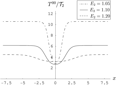
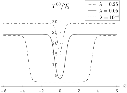
Figure 2: The energy density of nonBPS D-brane $T^{00}/{\cal T}_{2}$ with negative tension for various $E_{2}^{2}$ (equivalently $\Pi^{01}/{\cal T}_{2}$) and $\lambda$. We choose $E_{1}=0.1$ and $B=0.9$. The left figure has a fixed $\lambda=0.05$ and three $E_{2}$’s: $E_{2}=1.05$ ($\Pi^{01}/{\cal T}_{2}$=0.123) for the dot-dashed line, $E_{2}=1.1$ ($\Pi^{01}/{\cal T}_{2}$=0.133) for the solid line, and $E_{2}=1.2$ ($\Pi^{01}/{\cal T}_{2}$=0.171) for the dashed line from the above. The right figure has a fixed $E_{2}=1.02$ and three $\lambda$’s: $\lambda=0.15$ for the dot-dashed line, $\lambda=0.05$ for the solid line, and $\lambda=0.00001$ for the dashed line from the above.

According to the profiles of negative energy density, the configuration near the origin $x=0$ resembles a hole in condensed matter physics, created in the background of strong constant electromagnetic field.

(ii) exponential : For the exponential type of deformation (2.31), the unstable vacuum at $T=0$ is connected to the true vacuum at $T=\infty$. In this sense, one may call the configuration as a half tachyon kink and an anti-half tachyon kink respectively for the positive and negative sign in the exponential. It is convenient to rewrite the corresponding function $f(x)$ in (3.31) as

$$f(\mp\kappa x)=\frac{1}{1+e^{\pm 2\kappa(x-x_{0})}},\qquad\kappa x_{0}=\pm\ln(2\pi\lambda),$$ (4.10)

where $x_{0}$ may be considered as the position of the (anti-)half tachyon kink.

From the shape of $f(x)$, we see that the energy density for the half tachyon kink is monotonically increasing as shown in Fig. 3. In this sense the half tachyon kink is a phase boundary stretched along the $x^{2}$-direction. In addition the fundamental string charge density $\Pi^{02}$ (4.7) is also monotonic.

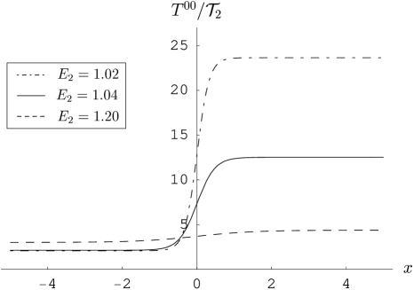
Figure 3: The energy density of tensionless half D-brane $T^{00}/{\cal T}_{2}$ for various $E_{2}^{2}$ (equivalently $\Pi^{01}/{\cal T}_{2}$). We choose $E_{1}=0.1$ and $B=0.9$, and due to translation, we can choose $\lambda=1/\sqrt{2\pi}$. The figure has three $E_{2}$’s: $E_{2}=1.02$ ($\Pi^{01}/{\cal T}_{2}$=0.115) for the dot-dashed line, $E_{2}=1.04$ ($\Pi^{01}/{\cal T}_{2}$=0.118) for the solid line, and $E_{2}=1.2$ ($\Pi^{01}/{\cal T}_{2}$=0.167) for the dashed line from the above.

A naive computation of tension of the half tachyon kink by integrating the energy density (4.5) from $x=-\infty$ to $x=+\infty$ leads to a divergence due to the contribution from the background energy proportional to $\int_{x_{0}}^{\infty}dx$. Therefore, it is reasonable to subtract it and we obtain the tension of the half tachyon kink as

$$\tilde{\cal T}_{1} =\int^{\infty}_{-\infty}dx\left[T^{00}-\frac{E_{2}^{2}B^{2}-E_{1}^{2}}{E_{2}^{2}-1}\left(\frac{\Pi^{01}}{E_{1}}\right)\right]-\int_{x_{0}}^{\infty}dx\left(-\frac{{\cal T}_{2}\sqrt{-{\cal Y}_{2}}}{E_{2}^{2}-1}\right)$$

$$=-\frac{{\cal T}_{2}\sqrt{-{\cal Y}_{2}}}{E_{2}^{2}-1}\left\{\int_{x_{0}}^{\infty}dx\left[\frac{1}{1+e^{2\kappa(x-x_{0})}}-1\right]+\int_{-\infty}^{x_{0}}dx\frac{1}{1+e^{2\kappa(x-x_{0})}}\right\}$$

$$=0.$$ (4.11)

Therefore the half tachyon kink is an object of vanishing energy and then is identified as a tensionless half brane ($\frac{1}{2}$brane) with thickness $1/2\kappa$. The profile of $\Pi^{02}(x)$ (4.7) is almost the same as the energy density (4.5). Suppose the low energy ($T=0$) configuration from $x=-\infty$ and the high energy ($T=\infty$) configuration from $x=+\infty$ are glued at $x_{0}$ with a sharp boundary. Then the formation of a smooth half tachyon kink suggests that the half phase boundary in the lower energy side gains both energy density and condensation of the fundamental string charge density, and the other half phase boundary in the high energy side loses exactly the same amount of the energy density and condensed fundamental string charge density. Note that this composite of tensionless $\frac{1}{2}$brane and fundamental strings has already been obtained as a half tachyon kink in DBI EFT, NCFT, and BSFT [9, 28, 13].

(iii) hyperbolic cosine : The hyperbolic cosine type tachyon profile in (iii) of (2.31) starts from $T=+\infty$, turns at a positive point $\lambda$, and then goes back to $T=+\infty$, which may be called a tachyon bounce (or a tachyon breather) in the classification of solitons. It could be interpreted as a composite of half tachyon kink and anti-half tachyon kink. Since the function $f(x)$ (3.32) is periodic in $\lambda$, we may assume $0\leq\lambda\leq 1/2$. The shape of the energy density is similar to that of the hyperbolic sine case as shown in Fig. 4 and we omit the details.

On integrating the localized part of the energy density, we obtain

$$\tilde{\cal T}_{1}=\frac{Q_{{\rm F}1}}{E_{2}}=\frac{\sqrt{2}{\cal T}_{2}}{\sqrt{E_{2}^{2}-1}}\ln(\sin^{2}\pi\lambda)<0.$$ (4.12)

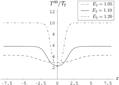
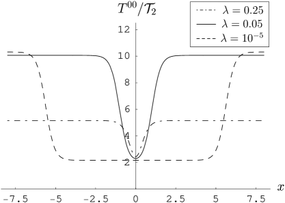
Figure 4: The energy density of tachyon bounce $T^{00}/{\cal T}_{2}$ with negative tension for various $E_{2}^{2}$ (equivalently $\Pi^{01}/{\cal T}_{2}$) and $\lambda$. We choose $E_{1}=0.1$ and $B=0.9$. The left figure has a fixed $\lambda=0.05$ and three $E_{2}$’s: $E_{2}=1.05$ ($-\Pi^{01}/{\cal T}_{2}$=0.117) for the dot-dashed line, $E_{2}=1.1$ ($-\Pi^{01}/{\cal T}_{2}$=0.127) for the solid line, and $E_{2}=1.2$ ($-\Pi^{01}/{\cal T}_{2}$=0.163) for the dashed line from the above. The right figure has a fixed $E_{2}=1.05$ and three $\lambda$’s: $\lambda=0.25$ for the dot-dashed line, $\lambda=0.05$ for the solid line, and $\lambda=0.00001$ for the dashed line from the above.

This object may be interpreted as a negative-tension brane of codimension-one, generated through de-condensing the background fundamental strings with a positive constant energy density. The hyperbolic cosine type tachyon profile also suggests an interpretation as a composite of half brane and anti-half brane. As D${\bar{\rm D}}$ is unstable, this composite of $\frac{1}{2}$brane and anti-$\frac{1}{2}$brane may also be unstable. This possible instability is classically expressed in terms of increase of the minimum value of the tachyon field in the tachyon bounce configuration. The parallel component of localized fundamental string charge (4.7) is also negative, and it means that the fundamental strings are repelled at the site of composite as shown in the right graph of Fig. 3. Therefore, the obtained object is nothing but a composite of $\frac{1}{2}$brane and anti-$\frac{1}{2}$brane accompanying de-condensation of the background fundamental strings.

Let us briefly discuss the bosonic string case. The cases of exponential tachyon profile for positive $\lambda$ (3.26) and hyperbolic cosine profile (3.27) for $0<\lambda\leq 1/2$ show qualitatively the same regular behavior as those of superstrings, however the case of hyperbolic sine always involves singularity. As mentioned previously, this can easily be understood by unbounded nature of the tachyon potential in bosonic string theory for the region of negative tachyon in (2.31).

Though we considered only the case of D1 from an unstable D2, but the extension to the higher dimensional case of D$(p-1)$ from D$p$ is straightforward. The aforementioned negative-tension branes and tensionless half brane are obtained only with a component of overcritical electric field. As we have discussed, such configurations with overcritical electric field seem to be unavoidable in the context of BCFT and may need further study in the context of string theory beyond BCFT. Recently the topic of marginal deformations is systematically dealt in the OSFT [38, 39], so will be the case of the obtained new tachyon vertices with the development of constant electromagnetic field. When the quantum radiations are taken into account including perturbative closed string modes such as gravitons, dilatons, and antisymmetric tensor fields, dynamical evolution of the negative-tension branes and tensionless half brane may become a more intriguing topic.

Finally, let us comment on the results in other approaches such as DBI EFT and NCFT with 1/cosh tachyon potential [9, 25, 28]. If we compare the physical quantities $T^{\mu\nu}(x)$ and $\Pi^{\mu\nu}(x)$ in the BCFT for superstrings with those in DBI EFT and NCFT with $1/\cosh$ tachyon potential, the BCFT results coincide exactly with the EFT results for the case of exponential type tachyon profile ((ii) of (2.31)) [9, 25, 28]. For hyperbolic sine ((i) of (2.31)) and hyperbolic cosine ((iii) of (2.31)) cases, the $x$-dependent part of physical quantities match qualitatively but do not exactly coincide with those of DBI EFT and NCFT.

5 Conclusions

In this paper, we considered a flat unstable D$p$-brane ($p\geq 2$) in the presence of a large constant electromagnetic field in the framework of BCFT. Specifically, we studied the case that the electromagnetic field satisfies the following three conditions: first, a constant electric field is turned on along the $x^{1}$ direction ($E_{1}\neq 0$); second, the determinant of the matrix $(\eta+F)$ is negative so that it lies in the physical region ($-\det(\eta+F)>0$); third, the 11-component of its cofactor is positive to the large electromagnetic field ($C^{11}>0$). For the simplest case, $p=2$, these conditions reduce to $E_{1}\neq 0$, $1-E_{1}^{2}-E_{2}^{2}+B^{2}>0$, and $|E_{2}|>1$, respectively. In the background of such electromagnetic fields, we identified exactly marginal deformations depending on the spatial coordinate $x^{1}$, which correspond to tachyon profiles of hyperbolic sine, exponential, and hyperbolic cosine types. The corresponding boundary states were constructed by utilizing T-duality approach and also by directly solving the overlap conditions in BCFT.

For these boundary states, we calculated the energy-momentum tensor and the fundamental string current density. Boundary states for the tachyon profiles of hyperbolic sine, exponential, and hyperbolic cosine correspond to nonBPS topological kink, half kink, and bounce in the effective field theories (DBI, NCFT, BSFT), respectively. In superstring theories, the first and third configurations have negative tensions and the second configuration gives tensionless half brane connecting the perturbative string vacuum and one of the true tachyon vacua.

The result obtained here in the BCFT description completes identifying all possible codimension-one static solutions on an unstable D$p$-brane in the presence of a constant electromagnetic field. Without an electromagnetic field, there exists a unique static solution of which the tachyon profile is sinusoidal with the period $2\pi$ [3, 1]. When a constant electromagnetic field is turned on, the spectrum of static solutions becomes rich; there are five types of solutions for $p\geq 2$, as summarized in the Table 1. This result coincides with that from DBI type EFT [9, 25], NCFT [28], and BSFT [13]. The detailed forms of the energy-momentum tensor and the fundamental string current density in the BCFT are qualitatively in agreement with those of the EFTs for cosine (sine), hyperbolic sine, and hyperbolic cosine types of tachyon profiles. For the linear and the exponential types, the physical quantities in the BCFT are exactly the same as those in the EFTs.

range of electromagnetic field	tachyon profile	interpretation
$C^{11}<0$, $-\det(\eta+F)>0$	cosine (sine)	array of D$(p-1)({\rm F}){\bar{\rm D}}(p-1)$(F)
$C^{11}<0$, $-\det(\eta+F)\rightarrow 0^{+}$	linear	single BPS D($p-1$)(F)
$C^{11}>0$, $-\det(\eta+F)>0$	hyperbolic sine	negative tension brane
$C^{11}>0$, $-\det(\eta+F)>0$	exponential	tensionless half brane
$C^{11}>0$, $-\det(\eta+F)>0$	hyperbolic cosine	negative tension brane

Table 1: List of all of the static solutions depending on a single spatial coordinate in the presence of constant electromagnetic field. When the spatial coordinate is $x^{1}$, the electric field along that direction should be turned on, $E_{1}\neq 0$.

Appendix A Exponential Type Tachyon Vertex Operator in BCFT for Superstrings

In $\sigma$-model approach to string theory, partition function of the worldsheet action gives the spacetime action and the couplings are interpreted as spacetime fields [40]. In relation to the static tachyon configuration, exact tachyon potential and tension of the lower-dimensional D-brane were obtained from the disk partition function in BSFT [11]. The similar procedure was adapted to the worldsheet action (2.1) with exactly marginal tachyon vertex operators. By identifying the worldsheet partition function with the spacetime action in bosonic string and superstring theory, the spacetime energy-momentum tensor without electromagnetic fields was obtained [29].

In this appendix we revisit BCFT for superstrings with the exponential type tachyon profile in (2.31) by employing the $\sigma$-model approach. The calculation in bosonic string theory was given in [41]. According to the procedure suggested by Ref. [29], we read the energy-momentum tensor and fundamental string current density of the unstable system with exponential type tachyon vertex operator by equating the spacetime action with the disk partition function of worldsheet theory.

The BCFT for superstrings is distinguished from that for bosonic string theory by introduction of worldsheet fermions and the form of worldsheet action is given in (2.19). Here we use the coordinate $z$ on the unit disk,

$$z=\frac{1+iw}{1-iw}.$$ (A.1)

From the action (2.19), we again read the worldsheet energy-momentum tensor

$$T(z)=-\partial X^{\mu}\partial X_{\mu}(z)-\frac{1}{2}\psi^{\mu}\partial\psi_{\mu}(z).$$ (A.2)

Under the deformed boundary conditions, (2.2) and (2.21), the correlation functions on the unit disk are given by

$$\langle X^{\mu}(z_{1})X^{\nu}(z_{2})\rangle_{A}= -\eta^{\mu\nu}\ln\mid z_{1}-z_{2}\mid+\eta^{\mu\nu}\ln\mid z_{1}\bar{z_{2}}-1\mid$$

$$-G^{\mu\nu}\ln\mid z_{1}\bar{z_{2}}-1\mid^{2}-\theta^{\mu\nu}\ln\left(\frac{z_{1}\bar{z_{2}}-1}{\bar{z_{1}}z_{2}-1}\right),$$ (A.3)

$$\langle\psi^{\mu}(z)\psi^{\nu}(z^{\prime})\rangle= \frac{\eta^{\mu\nu}}{z-z^{\prime}},\qquad\quad\langle{\bar{\psi}}^{\mu}({\bar{z}}){\bar{\psi}}^{\nu}({\bar{z}}^{\prime})\rangle=\frac{\eta^{\mu\nu}}{{\bar{z}}-{\bar{z}}^{\prime}},$$ (A.4)

$$\langle\psi^{\mu}(z){\bar{\psi}}^{\nu}({\bar{z}}^{\prime})\rangle= \left[\frac{1}{\eta-F}(\eta+F)\eta^{-1}\right]^{\mu\nu}\frac{1}{z-{\bar{z}}^{\prime}}.$$ (A.5)

The two-point function of $\Psi$ at the boundary is the usual one with the open string metric (2.13),

$$\langle\Psi^{\mu}(t_{1})\Psi^{\nu}(t_{2})\rangle=\frac{G^{\mu\nu}}{t_{1}-t_{2}},$$ (A.6)

where $t_{1}$ and $t_{2}$ represent the boundary coordinates on the unit disk, and the operator product expansion (OPE) for $\psi$ and $\Psi$ becomes

$$\psi^{\mu}(z)\Psi^{\nu}(t)\sim(G^{\mu\nu}-\theta^{\mu\nu})\frac{1}{z-t}.$$ (A.7)

We turn on a real tachyon field of exponential type, which is represented by the boundary interaction,

$$S_{T}=\int_{\partial\Sigma}dtd\theta\,T({\bf X}),\qquad T({\bf X})=\sqrt{2}\lambda\exp(ik_{\mu}{\bf X}^{\mu})\otimes\sigma_{1},$$ (A.8)

where we introduced the superfield ${\bf X}^{\mu}=X^{\mu}+i\sqrt{2}\theta\Psi^{\mu}$ with boundary Grassmann coordinate $\theta$ and $\sigma_{1}$ is the Chan-Paton factor in (2.22). The corresponding vertex in the zero-picture is obtained by integrating over $\theta$,

$$V_{T}=-2\lambda\,k\cdot\Psi\exp(ik_{\mu}X^{\mu})\otimes\sigma_{1}.$$ (A.9)

The marginality condition for the configurations with single spatial coordinate dependence (2.29) determines the value of $k^{\mu}$ in the tachyon vertex operator (A.9), which is the same as (2.30) for superstrings.

For later convenience, we write the two-point function of the superfield ${\bf X}^{1}$ on the boundary from (A.3) and (A.5),

$$\langle{\bf X}^{1}(z_{1},\theta_{1}){\bf X}^{1}(z_{2},\theta_{2})\rangle=-G^{11}\ln|z_{12}|^{2},$$ (A.10)

where $z_{12}=z_{1}-z_{2}-i\sqrt{z_{1}z_{2}}\theta_{1}\theta_{2}$.

From now on we compute the energy-momentum tensor and the fundamental string current density according to the procedure of Ref. [29]. The energy-momentum tensor in BCFT can be read from partition function of worldsheet theory coupled to background gravity [29],

$$S=Z_{{\rm disk}}\sim\int[dX][d\psi]e^{-S_{\rm w}-S_{T}},$$ (A.11)

where $Z_{{\rm disk}}$ is the disk partition function, and we replaced the flat metric $\eta_{\mu\nu}$ to $S_{\rm w}$ with the generic curved spacetime metric $g_{\mu\nu}$. Then we have the energy-momentum tensor in flat spacetime:

$$T_{\mu\nu}\equiv-\frac{2}{\sqrt{-g}}\left.\frac{\delta S}{\delta g^{\mu\nu}}\right|_{g_{\mu\nu}=\eta_{\mu\nu}}=K\sqrt{-\mathcal{Y}_{p}}\left[\eta_{\mu\nu}B(x)+A_{(\mu\nu)}(x)\right],$$ (A.12)

where $A_{(\mu\nu)}$ denotes the symmetric part of $A_{\mu\nu}$ and

$$B(x^{1})= -\frac{1}{\sqrt{-\mathcal{Y}_{p}}}\int[dX^{\prime}][d\psi]P\exp(-S_{0}-S_{A}-S_{T})=-\langle P\exp(-S_{T})\rangle_{A},$$ (A.13)

$$A^{\mu\nu}(x^{1})= -\frac{1}{\sqrt{-\mathcal{Y}_{p}}}\int[dX^{\prime}][d\psi]:(2\partial{X^{\prime}}^{\mu}\bar{\partial}{X^{\prime}}^{\nu}(0)+\psi^{\mu}\bar{\partial}\psi^{\nu}(0)+\bar{\psi}^{\mu}\partial\bar{\psi}^{\nu}(0)):$$

$$\quad\times P\exp(-S_{0}-S_{A}-S_{T})$$

$$= -\frac{1}{\sqrt{-\mathcal{Y}_{p}}}\left\langle:(2\partial{X^{\prime}}^{\mu}\bar{\partial}{X^{\prime}}^{\nu}(0)+\psi^{\mu}\bar{\partial}\psi^{\nu}(0)+\bar{\psi}^{\mu}\partial\bar{\psi}^{\nu}(0)):P\exp(-S_{T})\right\rangle_{A}.$$ (A.14)

Note that we split $X^{\mu}$ into the center of mass coordinate $x^{\mu}$ and fluctuation $X^{{}^{\prime}\mu}$, i.e., $X^{\mu}=x^{\mu}+X^{{}^{\prime}\mu}$, and $\langle\cdots\rangle_{A}$ denotes the vacuum expectation value in the presence of the U(1) gauge field on the unit disk with normalization

$$\langle 1\rangle_{A}=\sqrt{-\mathcal{Y}_{p}}\,.$$ (A.15)

In the calculation of $A^{\mu\nu}$ in (A.13), we follow the reference [5] and suppose that only the even part in $\sigma_{1}$ contributes to the result,

$$\left\langle\cdots P\exp(-S_{T})\right\rangle_{A}=\left\langle\cdots P\exp(-S_{T})\right\rangle_{A}\Big{|}_{\sigma_{1}-{\rm even}}.$$ (A.16)

First we calculate $B(x^{1})$. Using the two-point function (A.10), we have

$$B(x^{1})= -\sum_{n=0}^{\infty}(2\sqrt{2}\pi\lambda e^{\kappa x^{1}})^{2n}\int\prod_{i=1}^{2n}\frac{dt_{i}}{2\pi}d\theta_{i}\Theta(t_{1}-t_{2})\cdots\Theta(t_{2n-1}-t_{2n})$$

$$\hskip 119.50157pt\times\prod_{i<j}|e^{it_{i}}-e^{it_{j}}-ie^{\frac{i}{2}(t_{i}+t_{j})\theta_{i}\theta_{j}}|$$

$$= -\sum_{n=0}^{\infty}(-4\pi^{2}\lambda^{2}e^{2\kappa x^{1}})^{n}$$

$$= -f(\kappa x^{1}).$$ (A.17)

Then we compute the function $A^{\mu\nu}$. Since the second and third terms in (A.14) vanish, (A.14) becomes

$$A^{\mu\nu}(x^{1})=\frac{-2}{\sqrt{-\mathcal{Y}_{p}}}\left\langle:\partial X^{\mu}\bar{\partial}X^{\nu}(0):P\exp(-S_{T})\right\rangle.$$ (A.18)

For the calculation of $A^{\mu\nu}(x)$ in (A.18), we introduce a different normal ordering for convenience,

$${}^{\circ}_{\circ}\partial X^{\mu}(z)\bar{\partial}X^{\nu}(z^{\prime}){}^{\circ}_{\circ}=\partial X^{\mu}(z)\bar{\partial}X^{\nu}(z^{\prime})-\partial\bar{\partial}^{{}^{\prime}}\langle X^{\mu}(z)X^{\nu}(z^{\prime})\rangle_{A}.$$ (A.19)

The relationship between the ordinary normal ordering and the new ordering (A.19) is given by

$$:\partial X^{\mu}(0)\bar{\partial}X^{\nu}(0):={}^{\circ}_{\circ}\partial X^{\mu}(0)\bar{\partial}X^{\nu}(0){}^{\circ}_{\circ}+G^{\mu\nu}+\theta^{\mu\nu}-\frac{1}{2}\eta^{\mu\nu},$$ (A.20)

and this leads to

$$A^{\mu\nu}(x^{1})= \frac{-2}{\sqrt{-\mathcal{Y}_{p}}}\left\langle\left({}^{\circ}_{\circ}\partial X^{\mu}\bar{\partial}X^{\nu}(0){}^{\circ}_{\circ}-\left(\frac{1}{2}\eta^{\mu\nu}-G^{\mu\nu}-\theta^{\mu\nu}\right)\right)P\exp(-S_{T})\right\rangle$$

$$= -2\left[\frac{1}{\sqrt{-\mathcal{Y}_{p}}}\left\langle{}^{\circ}_{\circ}\partial X^{\mu}\bar{\partial}X^{\nu}(0){}^{\circ}_{\circ}P\exp(-S_{T})\right\rangle-\left(\frac{1}{2}\eta^{\mu\nu}-G^{\mu\nu}-\theta^{\mu\nu}\right)f(\kappa x^{1})\right].$$ (A.21)

The first term is calculated as follows,

$$\frac{1}{\sqrt{-\mathcal{Y}_{p}}} \left\langle{}^{\circ}_{\circ}\partial X^{\mu}\bar{\partial}X^{\nu}(0){}^{\circ}_{\circ}P\exp(-S_{T})\right\rangle$$

$$= \sum_{n=1}^{\infty}(2\sqrt{2}\pi\lambda e^{\kappa x^{1}})^{2n}\int\prod_{i=1}^{2n}\frac{dt_{i}}{2\pi}d\theta_{i}\Theta(t_{1}-t_{2})\cdots\Theta(t_{2n-1}-t_{2n})$$

$$\quad\times\kappa^{2}(G^{\mu 1}+\theta^{\mu 1})(G^{\nu 1}-\theta^{\nu 1})\left(\sum_{k,l}e^{-t_{k}-t_{l}}\right)\prod_{i<j}|e^{it_{i}}-e^{it_{j}}-ie^{\frac{i}{2}(t_{i}+t_{j})\theta_{i}\theta_{j}}|$$

$$= 2\kappa^{2}(G^{\mu 1}+\theta^{\mu 1})(G^{\nu 1}-\theta^{\nu 1})\sum_{n=1}^{\infty}(-4\pi^{2}\lambda^{2}e^{2\kappa x^{1}})^{n}$$

$$= -\frac{1}{G^{11}}(G^{\mu 1}+\theta^{\mu 1})(G^{\nu 1}-\theta^{\nu 1})[f(\kappa x^{1})-1].$$ (A.22)

Finally we obtain

$$A^{\mu\nu}=2\left\{\frac{1}{G^{11}}(G^{\mu 1}+\theta^{\mu 1})(G^{\nu 1}-\theta^{\nu 1})[f(\kappa x^{1})-1]+\left(\frac{1}{2}\eta^{\mu\nu}-G^{\mu\nu}-\theta^{\mu\nu}\right)f(\kappa x^{1})\right\}.$$ (A.23)

As in the bosonic case [41], we determine the normalization constant in (A.12) as $K={\cal T}_{p}/2$. Substituting (A.17) and (A.23) into (A.12), we get the energy-momentum tensor (4.1). Similarly we obtain the fundamental string current density (4.2) which is proportional to the antisymmetric part of $A^{\mu\nu}$ (A.23).

For the sine and cosine type profiles, the above path integral method in BCFT is not well-defined due to singularities in OPE between two vertices. To obtain meaningful results for these cases, we have to adopt appropriate regularization schemes which await further development. This situation may have some similarity to the recently-obtained exactly marginal solutions in OSFT [38]. The exponential type marginal solution is well-defined since every OPE between two vertex operators is regular, while the sine and cosine type marginal solutions encounter singular behaviors of OPE between vertex operators.

References

- [1] For a review, see A. Sen, “Tachyon dynamics in open string theory,” Int. J. Mod. Phys. A 20, 5513 (2005) [arXiv:hep-th/0410103], and references therein.
- [2] A. Sen, “SO(32) spinors of type I and other solitons on brane-antibrane pair,” JHEP 9809, 023 (1998) [arXiv:hep-th/9808141].
- [3] A. Sen, “BPS D-branes on non-supersymmetric cycles,” JHEP 9812, 021 (1998) [arXiv:hep-th/9812031].
- [4] A. Sen, “Rolling tachyon,” JHEP 0204, 048 (2002) [arXiv:hep-th/0203211].
- [5] A. Sen, “Tachyon matter,” JHEP 0207, 065 (2002) [arXiv:hep-th/0203265].
- [6] A. Sen, “Descent relations among bosonic D-branes,” Int. J. Mod. Phys. A 14, 4061 (1999) [arXiv:hep-th/9902105].
- [7] A. Sen, “Field theory of tachyon matter,” Mod. Phys. Lett. A 17, 1797 (2002) [arXiv:hep-th/0204143].
- [8] N. Lambert, H. Liu and J. Maldacena, “Closed strings from decaying D-branes,” arXiv:hep-th/0303139.
- [9] C. Kim, Y. Kim and C. O. Lee, “Tachyon kinks,” JHEP 0305, 020 (2003) [arXiv:hep-th/0304180].
- [10] P. Brax, J. Mourad and D. A. Steer, “Tachyon kinks on non BPS D-branes,” Phys. Lett. B 575, 115 (2003) [arXiv:hep-th/0304197].
- [11] A. A. Gerasimov and S. L. Shatashvili, “On exact tachyon potential in open string field theory,” JHEP 0010, 034 (2000) [arXiv:hep-th/0009103]; D. Kutasov, M. Marino and G. W. Moore, “Some exact results on tachyon condensation in string field theory,” JHEP 0010, 045 (2000) [arXiv:hep-th/0009148]; D. Kutasov, M. Marino and G. W. Moore, “Remarks on tachyon condensation in superstring field theory,” arXiv:hep-th/0010108.
- [12] S. Sugimoto and S. Terashima, “Tachyon matter in boundary string field theory,” JHEP 0207, 025 (2002) [arXiv:hep-th/0205085]; J. A. Minahan, “Rolling the tachyon in super BSFT,” JHEP 0207, 030 (2002) [arXiv:hep-th/0205098]. A. Ishida, Y. Kim and S. Kouwn, “Homogeneous rolling tachyons in boundary string field theory,” Phys. Lett. B 638, 265 (2006) [arXiv:hep-th/0601208].
- [13] C. Kim, Y. Kim, O. K. Kwon and H. U. Yee, “Tachyon kinks in boundary string field theory,” JHEP 0603, 086 (2006) [arXiv:hep-th/0601206].
- [14] A. Maloney, A. Strominger and X. Yin, “S-brane thermodynamics,” JHEP 0310, 048 (2003) [arXiv:hep-th/0302146].
- [15] D. Kutasov and V. Niarchos, “Tachyon effective actions in open string theory,” Nucl. Phys. B 666, 56 (2003) [arXiv:hep-th/0304045].
- [16] E. Witten, “Bound states of strings and p-branes,” Nucl. Phys. B 460, 335 (1996) [arXiv:hep-th/9510135].
- [17] P. Yi, “Membranes from five-branes and fundamental strings from Dp branes,” Nucl. Phys. B 550, 214 (1999) [arXiv:hep-th/9901159].
- [18] G. W. Gibbons, K. Hori and P. Yi, “String fluid from unstable D-branes,” Nucl. Phys. B 596, 136 (2001) [arXiv:hep-th/0009061].
- [19] A. Sen, “Fundamental strings in open string theory at the tachyonic vacuum,” J. Math. Phys. 42, 2844 (2001) [arXiv:hep-th/0010240].
- [20] P. Mukhopadhyay and A. Sen, “Decay of unstable D-branes with electric field,” JHEP 0211, 047 (2002) [arXiv:hep-th/0208142].
- [21] G. Gibbons, K. Hashimoto and P. Yi, “Tachyon condensates, Carrollian contraction of Lorentz group, and fundamental strings,” JHEP 0209, 061 (2002) [arXiv:hep-th/0209034].
- [22] A. Ishida and S. Uehara, “Gauge fields on tachyon matter,” Phys. Lett. B 544, 353 (2002) [arXiv:hep-th/0206102].
- [23] S. J. Rey and S. Sugimoto, “Rolling tachyon with electric and magnetic fields: T-duality approach,” Phys. Rev. D 67, 086008 (2003) [arXiv:hep-th/0301049].
- [24] C. Kim, H. B. Kim, Y. Kim and O-K. Kwon, “Electromagnetic string fluid in rolling tachyon,” JHEP 0303, 008 (2003) [arXiv:hep-th/0301076]; C. Kim, H. B. Kim, Y. Kim, O-K. Kwon and C. O. Lee, “Unstable D-branes and string cosmology,” J. Korean Phys. Soc. 45, S181 (2004) [arXiv:hep-th/0404242].
- [25] C. Kim, Y. Kim, O-K. Kwon and C. O. Lee, “Tachyon kinks on unstable Dp-branes,” JHEP 0311, 034 (2003) [arXiv:hep-th/0305092].
- [26] A. Sen, “Open and closed strings from unstable D-branes,” Phys. Rev. D 68, 106003 (2003) [arXiv:hep-th/0305011].
- [27] R. Banerjee, Y. Kim and O-K. Kwon, “Noncommutative tachyon kinks as D(p-1)-branes from unstable D p-brane,” JHEP 0501, 023 (2005) [arXiv:hep-th/0407229].
- [28] Y. Kim, O-K. Kwon and C. O. Lee, “Domain walls in noncommutative field theories,” JHEP 0501, 032 (2005) [arXiv:hep-th/0411164].
- [29] F. Larsen, A. Naqvi and S. Terashima, “Rolling tachyons and decaying branes,” JHEP 0302, 039 (2003) [arXiv:hep-th/0212248].
- [30] C. G. . Callan, I. R. Klebanov, A. W. W. Ludwig and J. M. Maldacena, “Exact solution of a boundary conformal field theory,” Nucl. Phys. B 422, 417 (1994) [arXiv:hep-th/9402113].
- [31] J. Polchinski and L. Thorlacius, “Free fermion representation of a boundary conformal field theory,” Phys. Rev. D 50, 622 (1994) [arXiv:hep-th/9404008].
- [32] A. Recknagel and V. Schomerus, “Boundary deformation theory and moduli spaces of D-branes,” Nucl. Phys. B 545, 233 (1999) [arXiv:hep-th/9811237].
- [33] N. Ishibashi, “The boundary and crosscap states in conformal field theories,” Mod. Phys. Lett. A 4, 251 (1989).
- [34] A. Abouelsaood, C. G. . Callan, C. R. Nappi and S. A. Yost, “Open strings in background gauge fields,” Nucl. Phys. B 280, 599 (1987); C. G. . Callan, C. Lovelace, C. R. Nappi and S. A. Yost, “String loop corrections to beta functions,” Nucl. Phys. B 288, 525 (1987).
- [35] P. Di Vecchia and A. Liccardo, “D branes in string theory. I,” NATO Adv. Study Inst. Ser. C. Math. Phys. Sci. 556, 1 (2000) [arXiv:hep-th/9912161]; “D-branes in string theory. II,” arXiv:hep-th/9912275.
- [36] C. G. . Callan and I. R. Klebanov, “Exact C = 1 boundary conformal field theories,” Phys. Rev. Lett. 72, 1968 (1994) [arXiv:hep-th/9311092].
- [37] O. K. Kwon and P. Yi, “String fluid, tachyon matter, and domain walls,” JHEP 0309, 003 (2003) [arXiv:hep-th/0305229].
- [38] M. Schnabl, “Comments on marginal deformations in open string field theory,” Phys. Lett. B 654, 194 (2007) [arXiv:hep-th/0701248]; M. Kiermaier, Y. Okawa, L. Rastelli and B. Zwiebach, “Analytic solutions for marginal deformations in open string field theory,” arXiv:hep-th/0701249.
- [39] T. Erler, “Marginal Solutions for the Superstring,” JHEP 0707, 050 (2007) [arXiv:0704.0930 [hep-th]]; Y. Okawa, “Analytic solutions for marginal deformations in open superstring field theory,” JHEP 0709, 084 (2007) [arXiv:0704.0936 [hep-th]]; “Real analytic solutions for marginal deformations in open superstring field theory,” JHEP 0709, 082 (2007) [arXiv:0704.3612 [hep-th]]; E. Fuchs, M. Kroyter and R. Potting, “Marginal deformations in string field theory,” JHEP 0709, 101 (2007) [arXiv:0704.2222 [hep-th]]; E. Fuchs and M. Kroyter, “Marginal deformation for the photon in superstring field theory,” JHEP 0711, 005 (2007) [arXiv:0706.0717 [hep-th]]; M. Kiermaier and Y. Okawa, “Exact marginality in open string field theory: a general framework,” arXiv:0707.4472 [hep-th]; “General marginal deformations in open superstring field theory,” arXiv:0708.3394 [hep-th].
- [40] E. S. Fradkin and A. A. Tseytlin, “Quantum string theory effective action,” Nucl. Phys. B 261 (1985) 1; C. G. . Callan, E. J. Martinec, M. J. Perry and D. Friedan, “Strings in background fields,” Nucl. Phys. B 262, 593 (1985).
- [41] A. Ishida, Y. Kim, C. Kim and O. K. Kwon, “Lower Dimensional Branes in Boundary Conformal Field Theory,” J. Korean Phys. Soc. 50, S36 (2007) [arXiv:0801.3188 [hep-th]].