Direct evidence for inversion formula in multifractal financial volatility measure

Abstract

The inversion formula for conservative multifractal measures was unveiled mathematically a decade ago, which is however not well tested in real complex systems. In this Letter, we propose to verify the inversion formula using high-frequency turbulent financial data. We construct conservative volatility measure based on minutely S&P 500 index from 1982 to 1999 and its inverse measure of exit time. Both the direct and inverse measures exhibit nice multifractal nature, whose scaling ranges are not irrelevant. Empirical investigation shows that the inversion formula holds in financial markets.

In recent years, the concept of inverse statistics has attracted much attention in turbulence Jensen (1999); Biferale et al. (1999) as well as in financial markets Simonsen et al. (2002) based on time series analysis. The direct structure function concerns with the statistical moments of a physical quantity $g$ measured over a distance $s$ such that $S_{q}(s)=\langle g_{\|}(s)^{q}\rangle$. The multifractal nature of direct structure functions has been well documented in turbulence McCauley (1990); Frisch (1996); Anselmet et al. (1984), as well as in finance Vandewalle and Ausloos (1998); Ivanova and Ausloos (1999); Calvet and Fisher (2002), which is characterized by $S_{q}(s)\sim s^{\zeta(q)}$ with a nonlinear scaling function $\zeta(q)$. In contract, the inverse structure function is related to the exit distance, where the physical quantity fluctuation exceeds a prescribed value, such that $T_{p}(g)=\langle s^{p}(g)\rangle$. One can intuitively expect that there is a power law scaling stating that $T_{p}(g)\sim g^{\phi(p)}$, where $\phi(p)$ is also a nonlinear function. Furthermore, if $s\sim g^{1/h}$, Schmitt has shown that there is an inversion formula between the two types of scaling exponents such that $\zeta(q)=-p$ and $\phi(p)=-q$ Schmitt (2005). A similar intuitive derivation for the inversion formula is given for Laplacian random walks Hastings (2002).

The power-law scaling in inverse structure function was observed in the signals of two dimensional turbulence Biferale et al. (2001, 2003), in the synthetic velocity data of the GOY shell model Jensen (1999); Roux and Jensen (2004), and in the temperature and longitudinal and transverse velocity data in grid-generated turbulence Beaulac and Mydlarski (2004). However, this scaling behavior was not observed in other three dimensional turbulent flows from different experiments Biferale et al. (1999); Pearson and van de Water (2005); Zhou et al. (2006). The inversion formula for direct and inverse structure functions is verified for synthetic turbulence data of shell models Roux and Jensen (2004) but not for wind-tunnel turbulence data, which cover a range of Reynolds numbers ${\rm{Re}}=400-1000$ Pearson and van de Water (2005).

It is argued that Xu et al. (2006), the absence of inversion formula between the scaling exponents of direct and inverse structure functions is due to the facts that the velocity fluctuation is not a conservative quantity while a strict proof of the inversion formula was given for conservational multifractal measures Mandelbrot and Riedi (1997); Riedi and Mandelbrot (1997). It is noteworthy pointing out that, the inversion formula given by Roux and Jensen is obtained based on a special case of conservative measures, although they verified the inversion formula in the direct and inverse structure functions of shell models Roux and Jensen (2004). It is thus natural that Xu et al. proposed to test the inversion formula in the energy dissipation rate (a kind of conservative measure) rather than in the structure functions and they did found sound evidence in favor of the proof Xu et al. (2006).

The inversion formula was theoretically established for both discontinuous and continuous multifractal measures by Riedi and Mandelbrot Mandelbrot and Riedi (1997); Riedi and Mandelbrot (1997). Let $\mu$ be a probability measure on $[0,1]$ whose integral function $M(a)=\mu([0,a])$ is right-continuous and nondecreasing. Since the measure is self-similar, we have $\mu=\sum_{i=0}^{n}m_{i}\mu(w_{i}^{-1}(\cdot))$, where $w_{i}$’s are the similarity maps with scale contraction ratios $r_{i}\in(0,1)$ and $\sum_{i=1}^{n}m_{i}=1$ with $m_{i}>0$. The multifractal spectrum $f(\alpha)$ of measure $\mu$ can be obtained via the Legendre transform of $\tau$, which is defined by

$$\sum_{i=1}^{n}m_{i}^{q}r_{i}^{-\tau}=1~{}.$$ (1)

The inverse measure of $\mu^{*}$ can be defined as follows,

$$\mu^{*}=M^{*}(b)=\left\{\begin{array}[]{lll}\inf\{a:M(a)>b\}&&{\rm{if}}~{}b<1\\ 1&&{\rm{if}}~{}b=1\end{array}\right.,$$ (2)

where $M^{*}(b)$ is the inverse function of $M(a)$. Since $\mu$ is self-similar, its inverse measure $\mu^{*}$ is also self-similar with ratios $r_{i}^{*}=m_{i}$ and probabilities $m_{i}^{*}=r_{i}$, whose multifractal spectrum $f^{*}(\alpha^{*})$ is the Legendre transform of $\theta$, which is defined implicitly by

$$\sum_{i=1}^{n}(m^{*}_{i})^{p}(r_{i}^{*})^{-\theta}=1~{}.$$ (3)

The inversion formula follows immediately that

$$\left\{\begin{array}[]{lll}\tau(q)&=&-p\\ \theta(p)&=&-q\end{array}\right..$$ (4)

Equivalently, we have

$$\tau(q)=-\theta^{-1}(-q)$$ (5)

or

$$\theta(p)=-\tau^{-1}(-p)~{}.$$ (6)

These two equivalent relations are testable. Following this line, the inversion formula was verified in Xu et al. (2006) with high-Reynolds turbulence data collected at the S1 ONERA wind tunnel Anselmet et al. (1984), which is however the only evidence. Due to the well documented analogues between turbulent flows and financial markets Mantegna and Stanley (2000), in this letter, we propose to test the inversion formula in financial markets using high-frequency historical data of the S&P 500 index. Our data consist of 18-year minutely prices spanning from 1 January, 1982 to 31 December, 1999 with a total of 1.7 million data points. The minutely return $r(t)$ is calculated as follows,

$$r(t)=\ln[I(t)/I(t-1)]~{},$$ (7)

where $\{I(t):t=1,\cdots,T\}$ is the time series of minutely S&P 500 index.

We first construct the direct volatility measure and investigate its multifractal nature. The absolute return is utilized as a proxy for volatility such that $v(t)=|r(t)|$. According to the partition function method for multifractal analysis, the series is firstly covered by $N$ boxes with identical size $s=T/N$. The sizes of the boxes are chosen such that the number of boxes of each size is an integer to cover the whole time series. On each box, we construct the direct measure as

$$\mu_{n}(s)=\frac{1}{V}\sum_{t=(n-1)s+1}^{ns}v(t),$$ (8)

where $V=\sum_{t=1}^{T}v(t)$ and $n=1,\cdots,N$. By construction, this volatility measure $\mu$ is conservative. The presence of multifractality in $\mu$ has been confirmed based on the multiplier method utilizing the same data set of the minutely S&P 500 index Jiang and Zhou (2007). Alternatively, the volatility measure $\mu$ of Chinese stocks and indexes exhibits multifractal behavior based on the partition function approach Jiang and Zhou (2008).

For order $q$, the direct partition function $\chi_{q}(s)$ can be estimated using

$$\chi_{q}(s)=\sum_{n=1}^{N}[\mu_{n}(s)]^{q}~{}.$$ (9)

When $\mu\ll 1$ and $q\gg 1$, the estimation of the partition function $\chi$ will be very difficult since the value is so small that it is “out of the memory”. To overcome this problem, we can calculate the logarithm of the partition function $\ln\chi_{q}(s)$ rather than the partition function itself. A simple manipulation results in the following formula

$$\ln\chi_{q}(s)=\ln\sum_{n=1}^{N}\left[\frac{\mu_{n}(s)}{\mu_{\max}}\right]^{q}+q\ln\mu_{\max}~{},$$ (10)

where $\mu_{\max}=\max\{\mu_{n}:n=1,\cdots,N\}$. This trick applies for the calculation of inverse partition functions as well.

Figure 1 plots $[\chi_{q}(s)]^{1/q-1}$ as a function of box size $s$ for different orders. Sound power laws are observed for each partition function such that

$$\chi_{q}(s)\sim s^{\tau(q)}~{},$$ (11)

in which the scaling range spans about three orders of magnitude. The scaling exponent $\tau(q)$ can be estimated through a power-law fit to the data in the scaling range. We will see that $\tau(q)$ is a nonlinear function, confirming the presence of multifractality in the direct volatility measure.

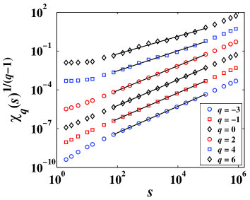
Figure 1: (color online.) Dependence of $\chi_{q}(s)^{1/q-1}$ as a function of box size $s$ for $q=-3$, $q=-1$, $q=0$, $q=4$, and $q=6$. The curves have been translated vertically by a factor of 0.001, 0.01, 0.1, 10, and 100 in turn for better visibility. The solid lines are power-law fits in the scaling range.

We now investigate the scaling behavior of inverse partition function of exit times. For each threshold $\Delta{v}$, a sequence of exit times $s_{j}(\Delta v)$ can be determined successively from $j=1$ to $j=J$ by

$$\sum_{k=1}^{j}s_{k}=\inf\left\{t:\int_{0}^{t}\nu(t)dt\geqslant j\Delta v\right\}~{},$$ (12)

where $\nu(t)=v(t)$ for $t\in[t,t+1)$. The inverse measure is defined as the normalized exit time

$$\mu^{*}_{j}(\Delta{v})=s_{j}/T~{},$$ (13)

and the inverse partition function can be determined as follows

$$\chi_{p}^{*}(\Delta{v})=\sum_{j=1}^{J}\left[\mu^{*}_{j}(\Delta{v})\right]^{p}~{},$$ (14)

where

$$J=\left[\frac{1}{\Delta{v}}\int_{0}^{T}\nu(t)dt\right]~{}.$$ (15)

Figure 2 shows the dependence of $\chi^{*}_{p}(\Delta v)^{1/(p-1)}$ on the threshold values $\Delta{v}$ for different values of $p$. Power-law scaling can be observed

$$\chi_{p}^{*}(s)\sim\Delta v^{\theta(p)}~{}.$$ (16)

where the scaling range covers about three orders of magnitude. The straight lines are the best fits to the data in the scaling range, whose slopes correspond to the exponents $\theta(p)/(p-1)$. We note that the two scaling ranges $(s_{1},s_{2})$ and $(\Delta{v}_{1},\Delta{v}_{2})$ for direct and inverse partition functions are related by

$$\Delta{v}=s\times{v}_{\rm{mean}}~{},$$ (17)

where $v_{\rm{mean}}=2.69\times 10^{-4}$. Specifically, we find that $\Delta{v}_{1}\approx{s_{1}}\times{v}_{\rm{mean}}$ and $\Delta{v}_{2}\approx{s_{2}}\times{v}_{\rm{mean}}$. This puts forward sound evidence upon the determination of the scaling laws.

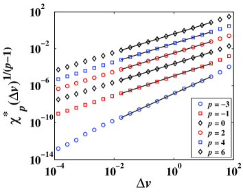
Figure 2: (color online.) Dependence of $\chi^{*}_{p}(\Delta v)^{1/p-1}$ on the thresholds $\Delta v$. The same translated processes are also performed on the data points of $p=-3$, $p=-1$, $p=0$, $p=4$, and $p=6$. The solid lines are the best fits to the data.

A subtle issue concerning negative moments arises, which is related to the probability density functions (PDFs) of volatility and exit time respectively. The volatility of S&P 500 index is log-normally distributed in the center followed by a power-law tail for large volatilities while the right tail seems truncated Cizeau et al. (1997); Liu et al. (1999). In addition, due to the construction of the volatility measure, $\mu(s)>0$ for large $s$ in the scaling range shown in Fig. 1. Therefore, negative moments can be estimated numerically. Taking into account the statistical significance of the estimation of partition functions L’vov et al. (1998); Zhou et al. (2006), we focus on $q\in[-4,8]$.

The PDFs of exit time defined in this letter have not been investigated before. Let us denote by $f(s)$ the PDF of exit times for a fixed threshold $\Delta{v}$. For comparison, we normalize the exit time by their standard deviation $\sigma(\Delta v)$ for each given $\Delta v$. Then the PDF of the normalized exit times $x=s/\sigma$ can be determined by

$$\rho(x)=\sigma f(x\sigma)~{}.$$ (18)

Figure 3 shows the empirical PDFs $\sigma f(x\sigma)$ of the normalized exit times $x=s/\sigma$ for different thresholds $\Delta{v}$. The PDFs at different thresholds cannot be superposed by the simple normalization procedure. As sketched in Fig. 3(a), the PDFs are strongly asymmetric and not log-normal, which differs remarkably from the situation of energy dissipation in three-dimensional fully developed turbulence showing roughly log-normal distribution Xu et al. (2006). More interestingly, the probability density functions show plateaus on the left tails, which ensures the existence of any negative moments. Figure 3(b) shows that the right tail relaxes exponentially for small thresholds or faster for large thresholds. This relaxation behavior is different from those exit times extracted from financial return series exhibiting a power-law tail Simonsen et al. (2002); Jensen et al. (2004, 2003a, 2003b); Zhou and Yuan (2005); Simonsen et al. (2007),

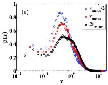
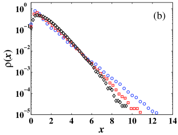
Figure 3: (color online.) Empirical probability density function $\rho(x)$ of the normalized exit time $x=s/\sigma$ for different thresholds $\Delta v=v_{\rm{mean}}/2$ ($\circ$), $v_{\rm{mean}}$ ($\Box$), and $2v_{\rm{mean}}$ ($\diamond$).

The power-law exponents $\tau(q)$ for direct partition functions are plotted as open circles in Fig. 4, while the exponents $\theta(q)$ are illustrated as triangles. Both $\tau(q)$ and $\theta(p)$ are nonlinear, indicating that the time series of volatility and exit time possess multifractal properties. The function $-\theta^{-1}(-q)$ is determined numerically from the $\theta(p)$ curve, which is plotted in Fig. 4 as a dashed line. We can find that the values of $-\theta^{-1}(-q)$ are in excellent agreement with the values of $\tau(p)$, which provides strong evidence supporting the inversion formula in Eq. (5). Similarly, the $-\tau^{-1}(-p)$ curve numerically obtained from the $\tau(p)$ function is depicted as a solid line, which coincides remarkably with the $\theta(q)$ curve. In other words, the inversion formula Eq. (6) also holds as expected. We note that the differences between the comparing curves are well within the error bars.

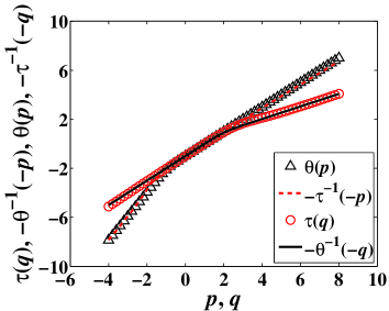
Figure 4: Testing the inversion formula in financial volatility.

In summary, we have attempted to test the inversion formula for conservative multifractal measures using high-frequency volatility data of the S&P 500 index. We have performed multifractal analysis on both volatility and exit time series based on the partition function method. Our investigation confirms that both direct and inverse partition functions exhibit nice multifractal properties. The two scaling ranges are consistent with each other. Furthermore, we found that the function $-\tau^{-1}(-p)$ extracted numerically from $\tau(q)$ overlaps with the $\theta(p)$ curve and the function $-\theta^{-1}(-q)$ determined from the $\theta(p)$ curve collapses on the $\tau(q)$ curve, which verifies the inversion formula. We also investigated for the first time the empirical distributions of exit time of financial volatility at different thresholds. The PDFs of exit time are nontrivial, which are neither log-normal nor power laws observed in other systems.