Capacity of Sparse Wideband Channels with
Partial Channel Feedback

Abstract

This paper studies the ergodic capacity of wideband multipath channels with limited feedback. Our work builds on recent results that have established the possibility of significant capacity gains in the wideband$/$low-${\sf{SNR}}$ regime when there is perfect channel state information (CSI) at the transmitter. Furthermore, the perfect CSI benchmark gain can be obtained with the feedback of just one bit per channel coefficient. However, the input signals used in these methods are peaky, that is, they have a large peak-to-average power ratios. Signal peakiness is related to channel coherence and many recent measurement campaigns show that, in contrast to previous assumptions, wideband channels exhibit a sparse multipath structure that naturally leads to coherence in time and frequency. In this work, we first show that even an instantaneous power constraint is sufficient to achieve the benchmark gain when perfect CSI is available at the receiver. In the more realistic non-coherent setting, we study the performance of a training-based signaling scheme. We show that multipath sparsity can be leveraged to achieve the benchmark gain under both average as well as instantaneous power constraints as long as the channel coherence scales at a sufficiently fast rate with signal space dimensions. We also present rules of thumb on choosing signaling parameters as a function of the channel parameters so that the full benefits of sparsity can be realized.

I Introduction

Recent research on the fundamental limits of wideband$/$low-${\sf{SNR}}$ communications has focused on the non-coherent regime where the impact of channel state information (CSI) on the achievable rates is critical. From a capacity perspective, spreading signals has been shown to be sub-optimal [1] and peaky or flash signaling schemes are necessary [2, 3] to achieve the non-coherent wideband capacity. Recent work by Zheng et al. [4] has emphasized the crucial role of channel coherence in the low-${\sf{SNR}}$ regime and the importance of implicit$/$explicit channel learning schemes that can bridge the gap between the coherent and the non-coherent extremes. However, these results have been derived based on an implicit assumption of rich multipath where the number of independent degrees of freedom (DoF) in the delay domain scale linearly with bandwidth.

Recent measurement campaigns in the case of ultrawideband systems show that the number of independent DoF do not scale linearly with bandwidth [5, 6, 7, 8, 9, 10, 11]. In fact, the physical layer channel model proposed by the IEEE 802.15 working group for ultrawideband communication systems exhibits sparsity in the delay domain (see for example, the measurement data in [12, p. 15]). Motivated by these works, we introduced the notion of multipath sparsity in [13] as a source of channel coherence and proposed a channel modeling framework to capture the impact of sparsity in delay and Doppler on achievable rates. The analysis in [13] shows that multipath sparsity can help in reducing$/$eliminating the need for peaky signaling in achieving wideband capacity.

In this work, we build on the results in [13] and study the impact of channel state feedback on achievable rates in sparse wideband channels. Although earlier works (for example [14, 15, 16] and references therein) have explored capacity with transmitter CSI, it is only recently [2, 17, 18] that the impact of feedback in the low-${\sf{SNR}}$, non-coherent regime has received attention. In particular, in the low-${\sf{SNR}}$ regime, it is shown in [17, 2] that with an average power constraint, the capacity gain with perfect transmitter and receiver CSI over the case when there is only perfect receiver CSI is $\log\left(\frac{1}{{\sf{SNR}}}\right)$. More interestingly, it is shown that a limited feedback scheme where only one bit per independent DoF is available at the transmitter can also achieve a gain of $\log\left(\frac{1}{{\sf{SNR}}}\right)$ [17, 2]. However, for both the optimal waterfilling scheme [19, 14] as well as the one bit limited feedback scheme, the input signal tends to be peaky (or bursty) in time, leading to a high peak-to-average power ratio, and difficulties from an implementation standpoint. The need to reliably estimate the channel at the receiver leads to the use of peaky training followed by communication in [17]. Similar results have also been reported in [18] where the authors study the optimization of the training length, average training power and spreading bandwidth in a wideband setting.

The focus of this work is on leveraging multipath sparsity to overcome or reduce the need for peaky signaling schemes. We work towards this goal by providing a concise description of the sparse channel model [13] in Sec. II. We then study the performance in the case where the receiver has perfect CSI and the transmitter has one bit (per independent DoF) in Sec. III. In contrast to [2, 17, 18] which study the performance only under an average (or long-term) power constraint, we also consider an instantaneous (or short-term) power constraint. We restrict our attention to causal signaling schemes that can be realized in practice. We show that an optimal threshold of the form ${\sf h_{t}}=\lambda\log\left(\frac{1}{{\sf{SNR}}}\right)$ for any $\lambda\in(0,1)$ provides a measure of achievable rate which behaves as $\left(1+{\sf h_{t}}\right){\sf{SNR}}$ in the wideband limit. Thus when $\lambda$ approaches $1$, we achieve the perfect transmitter CSI capacity which is the benchmark for all limited feedback schemes. We derive a sufficient condition under which this benchmark can be approached even with an instantaneous power constraint. A key parameter that determines this condition is ${\mathbf{E}}\left[{\sf D}_{\sf eff}\right]$, the average number of active independent channel dimensions, the number of independent channel coefficients that exceed the threshold in the power allocation scheme. In particular, with an instantaneous power constraint, the benchmark capacity gain is achieved when ${\mathbf{E}}\left[{\sf D}_{\sf eff}\right]-{\sf h_{t}}\rightarrow\infty$ as ${\sf{SNR}}\rightarrow 0$. We discuss the feasibility of the above condition when the channel is rich as well as sparse.

In Sec. IV, the focus is on the case where the receiver has no CSI a priori and a training-based signaling scheme is employed. Along the same lines as in [17, 18], we study the rates achievable with this scheme, albeit for sparse channels. With an average power constraint, it is shown that as long as the channel coherence dimension $\mathnormal{N_{c}}$ scales with ${\sf{SNR}}$ as $\mathnormal{N_{c}}=\frac{1}{{\sf{SNR}}^{\mu}}$ for some $\mu>1$, the rate achievable with the training scheme converges to the capacity with perfect transmitter CSI, the performance benchmark, in the wideband limit. Furthermore, this condition is achievable only when the channel is sparse and we provide guidelines on choosing the signal space parameters (signaling$/$packet duration, bandwidth and transmit power) such that $\mu>1$ is realized. The critical role of channel sparsity is further revealed when we impose an instantaneous power constraint. In contrast to peaky signaling that violates the finiteness constraint on the peak-to-average power, channel sparsity is necessary to realize the conditions required to approach the performance gain with an instantaneous power constraint: $\mu>1$ and ${\mathbf{E}}\left[{\sf D}_{\sf eff}\right]-{\sf h_{t}}\rightarrow\infty$. We summarize the paper in Sec. V by highlighting our contributions and placing them in the context of [2, 17, 18].

II System Model

In this section, we elucidate the model developed in [13] for sparse multipath channels. Our results are based on an orthogonal short-time Fourier (STF) signaling framework [20, 21] that naturally relates multipath sparsity in delay-Doppler to coherence in time and frequency.

II-A Sparse Multipath Channel Modeling

A discrete, physical multipath channel can be modeled as

$$y(t) = \int_{0}^{T_{m}}\!\!\!\int_{-\frac{W_{d}}{2}}^{\frac{W_{d}}{2}}h(\tau,\nu)x(t-\tau)e^{j2\pi\nu t}\,{\mathrm{d}}\nu\,{\mathrm{d}}\tau+w(t)$$ (1)

$$h(\tau,\nu) = \sum_{n}\beta_{n}\delta(\tau-\tau_{n})\delta(\nu-\nu_{n}),{\hskip 14.45377pt}y(t)=\sum_{n}\beta_{n}x(t-\tau_{n})e^{j2\pi\nu_{n}t}+w(t)$$ (2)

where $h(\tau,\nu)$ is the delay-Doppler spreading function of the channel, $\beta_{n}$, $\tau_{n}\in[0,T_{m}]$ and $\nu_{n}\in[-W_{d}/2,W_{d}/2]$ denote the complex path gain, delay and Doppler shift associated with the $n$-th path. $T_{m}$ and $W_{d}$ denote the delay and the Doppler spreads, respectively. The quantities $x(t),y(t)$ and $w(t)$ denote the transmitted, received and additive white Gaussian noise waveforms, respectively. Throughout this paper, we assume an underspread channel where $T_{m}W_{d}\ll 1$.

We use a virtual representation [22, 23] of the physical model in (2) that captures the channel characteristics in terms of resolvable paths and greatly facilitates system analysis from a communication-theoretic perspective. The virtual representation uniformly samples the multipath in delay and Doppler at a resolution commensurate with signaling bandwidth $W$ and signaling duration $T$, respectively. Thus, we have

$$y(t) = \sum_{\ell=0}^{L}\sum_{m=-M}^{M}h_{\ell,m}x(t-\ell/W)e^{j2\pi mt/T}+w(t)$$ (3)

$$h_{\ell,m} \approx \sum_{n\in S_{\tau,\ell}\hskip 1.4457pt\cap\hskip 1.4457ptS_{\nu,m}}\beta_{n}$$ (4)

where $L=\lceil T_{m}W\rceil$ and $M=\lceil TW_{d}/2\rceil$. The sampled representation (3) is linear and is characterized by the virtual delay-Doppler channel coefficients $\{h_{\ell,m}\}$ in (4). Each $h_{\ell,m}$ consists of the sum of gains of all paths whose delay and Doppler shifts lie within the $(\ell,m)$-th delay-Doppler resolution bin $S_{\tau,\ell}\cap S_{\nu,m}$ of size $\Delta\tau\times\Delta\nu$, $\Delta\tau=\frac{1}{W},\Delta\nu=\frac{1}{T}$ as illustrated in Fig. 1(a). Distinct $h_{\ell,m}$’s correspond to approximately disjoint subsets of paths and are hence approximately statistically independent. In this work, we assume that the channel coefficients $\{h_{\ell,m}\}$ are perfectly independent. We also assume Rayleigh fading in which $\{h_{\ell,m}\}$ are zero-mean Gaussian random variables.

Let $D$ denote the number of non-zero channel coefficients that reflects the (dominant) statistically independent DoF in the channel and also signifies the delay-Doppler diversity afforded by the channel [22]. We decompose $D$ as $D=D_{T}D_{W}$ where $D_{T}$ denotes the Doppler$/$time diversity and $D_{W}$ denotes the frequency$/$delay diversity. The channel DoF or delay-Doppler diversity is bounded as

$$D = D_{T}D_{W}\hskip 1.4457pt\leq\hskip 1.4457ptD_{\max}\triangleq D_{T,\hskip 1.4457pt\max}D_{W,\hskip 1.4457pt\max}$$ (5)

$$D_{T,\hskip 1.4457pt\max} = \left\lceil TW_{d}\right\rceil\ ,\ D_{W,\hskip 1.4457pt\max}=\left\lceil T_{m}W\right\rceil$$ (6)

where $D_{T,\hskip 1.4457pt\max}$ denotes the maximum Doppler diversity and $D_{W,\hskip 1.4457pt\max}$ denotes the maximum delay diversity. Note that $D_{T,\hskip 1.4457pt\max}$ and $D_{W,\hskip 1.4457pt\max}$ increase linearly with $T$ and $W$, respectively, and thus represent a rich multipath environment in which each resolution bin in Fig. 1(a) corresponds to a dominant channel coefficient.

However, there is growing experimental evidence [5, 6, 7, 8, 9, 10, 11] that the dominant channel coefficients get sparser in delay as the bandwidth increases. Furthermore, we are also interested in modeling scenarios with Doppler effects, due to motion. In such cases, as we consider large bandwidths and$/$or long signaling durations, the resolution of paths in both delay and Doppler domains gets finer, leading to the scenario in Fig. 1(a) where the delay-Doppler resolution bins are sparsely populated with paths, i.e. $D\ll D_{\max}$.

In this work, we model multipath sparsity by a sub-linear scaling of $D_{T}$ and $D_{W}$ with $T$ and $W$, respectively:

$$D_{W}\sim g_{1}(W)\ ,\ D_{T}\sim g_{2}(T)$$ (7)

where $g_{1}$ and $g_{2}$ are arbitrary sub-linear functions. As a concrete example, we will focus on a power-law scaling for the rest of this paper:

$$D_{T}=\left(TW_{d}\right)^{\delta_{1}},\hskip 3.61371pt\hskip 3.61371pt\hskip 3.61371ptD_{W}=\left(WT_{m}\right)^{\delta_{2}}$$ (8)

for some $\delta_{1},\delta_{2}\in(0,1)$. But the results derived here hold true for any general sub-linear scaling law. Note that (6) and (7) imply that in sparse multipath, the total number of delay-Doppler DoF, $D=D_{T}D_{W}$, scales sub-linearly with the signal space dimension $N=TW$.

Remark 1

With perfect CSI at the receiver, the parameter $D$ denotes the delay-Doppler diversity afforded by the channel, whereas with no CSI, it reflects the level of channel uncertainty; the number of channel parameters that need to be learned at the receiver for coherent processing.

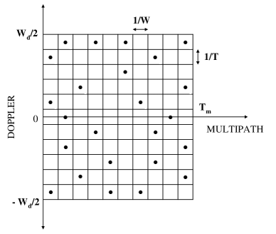
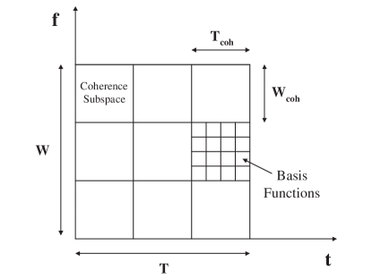
(a)	(b)

Figure 1: (a) Delay-doppler sampling commensurate with signaling bandwidth and duration. (b) Time-frequency coherence subspaces in STF signaling.

II-B Orthogonal Short-Time Fourier Signaling

We consider signaling using an orthonormal short-time Fourier (STF) basis [20, 21] that is a natural generalization of orthogonal frequency-division multiplexing (OFDM) for time-varying channels. An orthogonal STF basis $\{\phi_{\ell m}(t)\}$ for the signal space is generated from a fixed prototype waveform $g(t)$ via time and frequency shifts: $\phi_{\ell m}(t)=g(t-\ell T_{o})e^{j2\pi W_{o}t}$, where $T_{o}W_{o}=1$, $\ell=0,\cdots,N_{T}-1$, $m=0,\cdots,N_{W}-1$ and $N=N_{T}N_{W}=TW$ with $N_{T}=T/T_{o},N_{W}=W/W_{o}$. The transmitted signal can be represented as

$$x(t)=\sum\limits_{\ell=0}^{N_{T}-1}\sum\limits_{m=0}^{N_{W}-1}x_{\ell m}\phi_{\ell m}(t)\hskip 3.61371pt\hskip 3.61371pt\,\ \hskip 3.61371pt0\leq t\leq T$$ (9)

where $\{x_{\ell m}\}$ denote the $N$ transmitted symbols that are modulated onto the STF basis waveforms. The received signal is projected onto the STF basis waveforms to yield

$$y_{\ell m}=\langle y,\phi_{\ell m}\rangle=\sum\limits_{\ell^{{}^{\prime}},m^{{}^{\prime}}}h_{\ell m,\ell^{{}^{\prime}}m^{{}^{\prime}}}\;\ x_{\ell^{{}^{\prime}}m^{{}^{\prime}}}+w_{\ell m}.$$ (10)

We can represent the system using an $N$-dimensional matrix equation [20, 21]

$${\mathbf{y}}=\hskip 3.61371pt{\mathbf{H}}{\mathbf{x}}+{\mathbf{w}}$$ (11)

where ${\mathbf{w}}$ is the additive noise vector whose entries are i.i.d. ${\cal CN}(0,1)$. The $N\times N$ matrix $\mathbf{H}$ consists of the channel coefficients $\{h_{\ell m,\ell^{{}^{\prime}}m^{{}^{\prime}}}\}$ in (10). We assume that the input symbols that form the transmit codeword ${\mathbf{x}}$ satisfy an average power constraint

$$\frac{1}{T}\cdot{\mathbf{E}}\left[\|{\mathbf{x}}\|^{2}\right]\leq P.$$ (12)

Since there are $N=TW$ symbols per codeword, we define the parameter ${\sf{SNR}}$ (transmit energy per modulated symbol) for a given average transmit power $P$ as ${\sf{SNR}}=\frac{TP}{TW}=\frac{P}{W}$. In this work, the focus is on the wideband regime where ${\sf{SNR}}\rightarrow 0$ as $W\rightarrow\infty$ for a fixed $P$.

For sufficiently underspread channels, the parameters $T_{o}$ and $W_{o}$ can be matched to $T_{m}$ and $W_{d}$ so that the STF basis waveforms serve as approximate eigenfunctions of the channel [21, 20]; that is, (10) simplifies to $y_{\ell m}\approx h_{\ell m}x_{\ell m}+w_{\ell m}$. Thus the channel matrix $\mathbf{H}$ is approximately diagonal. In this work, we assume that $\mathbf{H}$ is exactly diagonal; that is,

$${\mathbf{H}}={\mathrm{diag}}\Big{[}\underbrace{{h}_{11}\cdots{h}_{1\mathnormal{N_{c}}}}_{{\mathrm{Subspace}}\hskip 3.61371pt1},\hskip 3.61371pt\underbrace{{h}_{21}\cdots{h}_{2\mathnormal{N_{c}}}}_{{\mathrm{Subspace}}\hskip 3.61371pt2}\hskip 3.61371pt\cdots\hskip 3.61371pt\underbrace{{h}_{D1}\cdots{h}_{D\mathnormal{N_{c}}}}_{{\mathrm{Subspace}}\hskip 3.61371ptD}\Big{]}.$$ (13)

The diagonal entries of $\mathbf{H}$ in (13) admit an intuitive block fading interpretation in terms of time-frequency coherence subspaces [20] illustrated in Fig. 1(b). The signal space is partitioned as $N=TW=\mathnormal{N_{c}}D$ where $D$ represents the number of statistically independent time-frequency coherence subspaces, reflecting the DoF in the channel, and $\mathnormal{N_{c}}$ represents the dimension of each coherence subspace, which we refer to as the coherence dimension. In the block fading model in (13), the channel coefficients over the $i$-th coherence subspace $h_{i1},\cdots,h_{i\mathnormal{N_{c}}}$ are assumed to be identical (denoted by $h_{i}$), whereas the coefficients across different coherence subspaces are independent and identically distributed. Thus, the channel is characterized by the $D$ distinct STF channel coefficients, $\{h_{i}\}$, that are i.i.d. zero-mean Gaussian random variables (Rayleigh fading) with (normalized) variance equal to ${\mathbf{E}}[|h_{i}|^{2}]=\sum_{n}{\mathbf{E}}[|\beta_{n}|^{2}]=1$ [20].

Using the DoF scaling for sparse channels in (7), the scaling behavior for the coherence dimension can be computed as

$$\mathnormal{W_{coh}} = \frac{W}{D_{W}}\sim f_{1}(W),\hskip 3.61371pt\hskip 3.61371pt\hskip 3.61371pt\mathnormal{T_{coh}}=\frac{T}{D_{T}}\sim f_{2}(T)$$ (14)

$$\mathnormal{N_{c}} = \mathnormal{W_{coh}}\mathnormal{T_{coh}}\sim f_{1}(W)f_{2}(T)$$ (15)

where $\mathnormal{T_{coh}}$ is the coherence time and $\mathnormal{W_{coh}}$ is the coherence bandwidth of the channel, as illustrated in Fig. 1(b). As a consequence of the sub-linearity of $g_{1}$ and $g_{2}$ in (7), $f_{1}$ and $f_{2}$ are also sub-linear. In particular, corresponding to the power-law scaling in (8), we obtain

$$\mathnormal{T_{coh}}=\frac{T^{1-\delta_{1}}}{W_{d}^{\delta_{1}}},\hskip 3.61371pt\hskip 3.61371pt\hskip 3.61371pt\mathnormal{W_{coh}}=\frac{W^{1-\delta_{2}}}{T_{m}^{\delta_{2}}}.$$ (16)

Remark 2

Note that when the channel is sparse, both $\mathnormal{N_{c}}$ and $D$ increase sub-linearly with $N$, whereas when the channel is rich, $D$ scales linearly with $N$, while $\mathnormal{N_{c}}$ is fixed.

In this work, the focus is on computing achievable rates in the non-coherent setting with feedback and as we will see in Sec. III and IV, the rates turn out to be a function only of the parameters $\mathnormal{N_{c}}$ and ${\sf{SNR}}$. Thus, in order to analyze the low-${\sf{SNR}}$ asymptotics, the following relation between $\mathnormal{N_{c}}$ and ${\sf{SNR}}$ $(=P/W)$ plays a key role:

$$\mathnormal{N_{c}}=\frac{1}{{\sf{SNR}}^{\mu}}\hskip 3.61371pt,\hskip 3.61371pt\hskip 3.61371pt\hskip 3.61371pt\mu>0$$ (17)

where the parameter $\mu$ reflects the level of channel coherence. We will revisit (17) and discuss its achievability and implications in Sec. IV.

III Achievable Rates with Perfect Receiver CSI and Limited Channel State Feedback

In this section, we study the scenario when there is perfect CSI at the receiver. We assume throughout this paper that both the transmitter and the receiver have statistical CSI - knowledge of $T_{m}$, $W_{d}$, $g_{1}$, $g_{2}$, $f_{1}$ and $f_{2}$ so that the scaling in $D$ and $\mathnormal{N_{c}}$ are known. On one extreme, with perfect receiver CSI and no transmitter CSI (no feedback), the coherent capacity per dimension (in nats/s/Hz) equals

$$C_{{\sf coh},0}({\sf{SNR}})=\sup\limits_{{\mathbf{Q}}\hskip 0.72229pt:\hskip 0.72229pt{\mathrm{Tr}}({\mathbf{Q}})\hskip 1.4457pt\leq\hskip 1.4457ptTP}\frac{{{\mathbf{E}}}\left[\log\det\left({\mathbf{I}}_{\mathnormal{N_{c}}D}+{\mathbf{H}}{\mathbf{Q}}{\mathbf{H}}^{H}\right)\right]}{\mathnormal{N_{c}}D}.$$ (18)

The optimization is over the set of $\mathnormal{N_{c}}D$-dimensional positive definite input covariance matrices $\mathbf{Q}={\mathbf{E}}\left[{\mathbf{x}}{\mathbf{x}}^{H}\right]$ satisfying the average power constraint in (12). Due to the diagonal nature of $\mathbf{H}$ in (13), the optimal $\mathbf{Q}$ is also diagonal. Furthermore, with no transmitter CSI, the uniform power allocation $\mathbf{Q}=\frac{TP}{\mathnormal{N_{c}}D}\hskip 1.4457pt{\mathbf{I}}_{\mathnormal{N_{c}}D}={\sf{SNR}}\cdot{\mathbf{I}}_{\mathnormal{N_{c}}D}$ achieves this optimum. The corresponding capacity in the limit of low-${\sf{SNR}}$ is [2, 4]

$$C_{{\sf coh},0}({\sf{SNR}})\approx{\sf{SNR}}-{\sf{SNR}}^{2}.$$ (19)

On the other extreme is the case of perfect receiver and transmitter CSI, where the receiver instantaneously feeds back all the channel coefficients, $\{h_{i}\}_{i=1}^{D}$, corresponding to the $D$ independent coherence subspaces to the transmitter. The optimum transmitter power allocation in this case is waterfilling [19, 14] over the different coherence subspaces. In the low-${\sf{SNR}}$ extreme, it is shown in [2, 17] that the capacity with perfect transmitter CSI scales as $\log\left(\frac{1}{{\sf{SNR}}}\right){\sf{SNR}}$. That is, the capacity gain (compared with the receiver CSI only case) is directly proportional to the waterfilling threshold, $h_{w}\sim\log\left(\frac{1}{{\sf{SNR}}}\right)$, and this gain serves as a benchmark for all limited feedback schemes. More interestingly, it is shown in [2, 17] that this maximum capacity gain can be achieved with just one bit of feedback per channel coefficient.

In the case of limited feedback, both the transmitter and the receiver have a priori knowledge of a common threshold denoted by ${\sf h_{t}}$. The receiver compares the channel strength ($|h_{i}|^{2},\hskip 3.61371pti=1,2,\cdots,D$) in each coherence subspace with ${\sf h_{t}}$, and feeds back

$$b_{i}=\begin{cases}1\hskip 3.61371pt\hskip 3.61371pt{\rm if}\hskip 3.61371pt\hskip 3.61371pt|h_{i}|^{2}\geq{\sf h_{t}}\\ 0\hskip 3.61371pt\hskip 3.61371pt{\rm if}\hskip 3.61371pt\hskip 3.61371pt|h_{i}|^{2}<{\sf h_{t}}.\end{cases}$$ (20)

At the transmitter, power allocation is uniform across the coherence subspaces for which $b_{i}=1$ and no power is allocated to those subspaces for which $b_{i}=0$. The input power allocation is conditioned on the partial CSI available at the transmitter (denoted by ${\sf CSI}$), which is $\{b_{i}\}_{i=1}^{D}$. This power allocation, which we still denote by $\mathbf{Q}$ with an abuse of notation, takes the form

$$\mathbf{Q}({\sf CSI}) = {\mathrm{diag}}\left({\mathbf{E}}[|x_{1}|^{2}|{\sf CSI}],{\mathbf{E}}[|x_{2}|^{2}|{\sf CSI}],\cdots,{\mathbf{E}}[|x_{N}|^{2}|{\sf CSI}]\right)$$ (21)

$$= {\mathrm{diag}}\big{(}\underbrace{q_{1},\cdots,q_{1}}_{\mathnormal{N_{c}}}\hskip 1.4457pt,\hskip 1.4457pt\underbrace{q_{2},\cdots,q_{2}}_{\mathnormal{N_{c}}}\hskip 1.4457pt,\cdots,\hskip 1.4457pt\underbrace{q_{D},\cdots,q_{D}}_{\mathnormal{N_{c}}}\big{)}$$ (22)

$$q_{i} = \mathnormal{P_{0}}\cdot\chi(|h_{i}|^{2}\geq{\sf h_{t}}).$$ (23)

The choice of $\mathnormal{P_{0}}$ depends on the type of power constraint and also on the nature of feedback. To explore this further, let ${\sf D}_{\sf eff}$ denote the number of active subspaces, those which exceed the threshold ${\sf h_{t}}$. We have

$${\sf D}_{\sf eff}=\sum\limits_{i=1}^{D}\chi(|h_{i}|^{2}\geq{\sf h_{t}})$$ (24)

$${\mathbf{E}}\left[{\sf D}_{\sf eff}\right]\stackrel{{\scriptstyle(a)}}{{=}}D{\mathbf{E}}\left[\chi(|h|^{2}\geq{\sf h_{t}})\right]\stackrel{{\scriptstyle(b)}}{{=}}De^{-{\sf h_{t}}}$$ (25)

where (a) is due to the fact that $\{h_{i}\}_{i=1}^{D}$ are i.i.d. and (b) is due to the fact that for a standard Gaussian, ${\mathbf{E}}\left[\chi(|h_{i}|^{2}\geq{\sf h_{t}})\right]={\mathrm{Pr}}\left(|h_{i}|^{2}\geq{\sf h_{t}}\right)=e^{-{\sf h_{t}}}$.

If we assume knowledge of $\{b_{i}\}_{i=1}^{D}$ at the beginning of each codeword, albeit non-causally, at the transmitter, then we can uniformly divide power among the active subspaces. That is

$$\mathnormal{P_{0,\sf nc}}=\frac{TP}{\mathnormal{N_{c}}{\sf D}_{\sf eff}}.$$ (26)

The rate achievable with this power allocation, denoted by $C_{{\sf coh},1,{\sf LT}}({\sf{SNR}})$, is

$$C_{{\sf coh},1,{\sf LT}}({\sf{SNR}})=\max\limits_{{\sf h_{t}}}\frac{1}{D}\sum_{i=1}^{D}{\mathbf{E}}\left[\log\left(1+\frac{TP}{\mathnormal{N_{c}}{\sf D}_{\sf eff}}\cdot\left|h_{i}\right|^{2}\right)\chi\left(|h_{i}|^{2}\geq{\sf h_{t}}\right)\right].$$ (27)

The power allocation in (26) satisfies the power constraint instantaneously as well as on average. To see this, note that

$$P_{{\sf inst},{\sf nc}}=\frac{\mathnormal{N_{c}}}{T}\sum\limits_{i=1}^{D}q_{i}=\frac{\mathnormal{N_{c}}}{T}\sum\limits_{i=1}^{D}\frac{TP}{\mathnormal{N_{c}}{\sf D}_{\sf eff}}\chi\left(|h_{i}|^{2}\geq{\sf h_{t}}\right)=P$$ (28)

and clearly ${\mathbf{E}}\left[P_{{\sf inst},{\sf nc}}\right]=P$ as well. The non-causality of the scheme is more relevant in the scenario when the receiver estimates the channel coefficients $\{h_{i}\}_{i=1}^{D}$ and feeds back $\{b_{i}\}_{i=1}^{D}$ based on these estimates. This motivates us to instead consider a causal power allocation scheme, one in which for all $i=1,\cdots,D$, $q_{i}$ in (23) depends on $b_{i}$ only through the indicator function and $\mathnormal{P_{0}}$ is independent of $\{b_{i}\}_{i=1}^{D}$. From (23), we have

$${\mathbf{E}}\left[\|{\mathbf{x}}\|^{2}\right]=\mathnormal{N_{c}}\sum\limits_{i=1}^{D}{\mathbf{E}}\left[q_{i}\right]=\mathnormal{N_{c}}\sum\limits_{i=1}^{D}\mathnormal{P_{0}}\cdot{\mathbf{E}}\left[\chi(|h_{i}|^{2}\geq{\sf h_{t}})\right]=\mathnormal{N_{c}}\mathnormal{P_{0}}{\mathbf{E}}\left[{\sf D}_{\sf eff}\right].$$ (29)

Thus to satisfy ${\mathbf{E}}\left[\|{\mathbf{x}}\|^{2}\right]\leq TP$, the power allocation for the causal scheme is given by

$$\mathnormal{P_{0,\sf c}}=\frac{TP}{\mathnormal{N_{c}}{\mathbf{E}}\left[{\sf D}_{\sf eff}\right]}=\frac{TP}{\mathnormal{N_{c}}De^{-{\sf h_{t}}}}$$ (30)

and the corresponding rate, $\widehat{C}_{{\sf coh},1,{\sf LT}}({\sf{SNR}})$, is given by

$$\widehat{C}_{{\sf coh},1,{\sf LT}}({\sf{SNR}})=\max\limits_{{\sf h_{t}}}\frac{1}{D}\sum_{i=1}^{D}{\mathbf{E}}\left[\log\left(1+\frac{TP}{\mathnormal{N_{c}}De^{-{\sf h_{t}}}}|h_{i}|^{2}\right)\chi(\left|h_{i}\right|^{2}\geq{\sf h_{t}})\right].$$ (31)

The causal power allocation policy in (30) satisfies the average power constraint but can have a large instantaneous power. This is because

$$P_{{\sf inst},{\sf c}}=\frac{\mathnormal{N_{c}}}{T}\sum\limits_{i=1}^{D}\frac{TP}{\mathnormal{N_{c}}De^{-{\sf h_{t}}}}\chi\left(|h_{i}|^{2}\geq{\sf h_{t}}\right)=\left(\frac{{\sf D}_{\sf eff}}{De^{-{\sf h_{t}}}}\right)P.$$ (32)

Thus ${\mathbf{E}}\left[P_{{\sf inst},{\sf c}}\right]=P$, but unlike (28), $P_{{\sf inst},{\sf c}}\in[0,\infty)$ depending on the choice of ${\sf h_{t}}$. We will address this issue in Sec. III-B, but first, we study the average power constraint case more carefully.

III-A Achievable Rates under Average Power Constraint

The following theorem establishes that a threshold of the form ${\sf h_{t}}\sim\lambda\log\left(\frac{1}{{\sf{SNR}}}\right)$ for some $\lambda\in(0,1)$ provides the solution to (31).

Theorem 1

Given any $\lambda\in(0,1)$, a causal on-off signaling scheme under an average power constraint achieves $\widehat{C}_{\sf LB}\leq\widehat{C}_{{\sf coh},1,{\sf LT}}({\sf{SNR}})\leq\widehat{C}_{\sf UB}$ with an optimal threshold of the form:

$$\lim\limits_{{\sf{SNR}}\rightarrow 0}\frac{{\sf h_{t}}}{\lambda\log\left(\frac{1}{{\sf{SNR}}}\right)}=1$$ (33)

where

$$\widehat{C}_{\sf UB} = {\sf{SNR}}^{\lambda}\cdot\left[\log\left(\textstyle{1+\lambda{\sf{SNR}}^{1-\lambda}\log\left(\frac{1}{{\sf{SNR}}}\right)}\right)+\log\left(\textstyle{1+\frac{{\sf{SNR}}^{1-\lambda}}{1+\lambda{\sf{SNR}}^{1-\lambda}\log\left(\frac{1}{{\sf{SNR}}}\right)}}\right)\right]$$ (34)

$$\widehat{C}_{\sf LB} = {\sf{SNR}}^{\lambda}\cdot\left[\log\left(\textstyle{1+\lambda{\sf{SNR}}^{1-\lambda}\log\left(\frac{1}{{\sf{SNR}}}\right)}\right)+\frac{1}{2}\log\left(\textstyle{1+\frac{2{\sf{SNR}}^{1-\lambda}}{1+\lambda{\sf{SNR}}^{1-\lambda}\log\left(\frac{1}{{\sf{SNR}}}\right)}}\right)\right].$$ (35)

Proof:

Starting from (31), we have

$$\widehat{C}_{{\sf coh},1,{\sf LT}}({\sf{SNR}}) = \max\limits_{{\sf h_{t}}}\frac{1}{D}\sum_{i=1}^{D}{\mathbf{E}}\left[\log\left(1+\frac{TP}{\mathnormal{N_{c}}De^{-{\sf h_{t}}}}|h_{i}|^{2}\right)\chi(\left|h_{i}\right|^{2}\geq{\sf h_{t}})\right]$$ (36)

$$\stackrel{{\scriptstyle(a)}}{{=}} {\mathbf{E}}\left[\log\left(1+{\sf{SNR}}\hskip 1.4457pte^{{\sf h_{t}}}\hskip 1.4457pt|h|^{2}\right)\hskip 1.4457pt\chi(\left|h\right|^{2}\geq{\sf h_{t}})\right]$$ (37)

where (a) follows from the fact that $\{h_{i}\}$ are i.i.d. ${\cal CN}(0,1)$ and $h$ is a generic i.i.d. ${\cal CN}(0,1)$ random variable. The expectation in (37) can be computed using [24, 4.337(1), p. 574]. With $\alpha\triangleq\frac{1+{\sf{SNR}}\hskip 1.4457pt{\sf h_{t}}\hskip 1.4457pte^{{\sf h_{t}}}}{{\sf{SNR}}\hskip 1.4457pte^{{\sf h_{t}}}}$, we have

$$\widehat{C}_{{\sf coh},1,{\sf LT}}({\sf{SNR}}) = e^{-{\sf h_{t}}}\cdot\left[\textstyle{\log\left(1+{\sf{SNR}}\hskip 1.4457pt{\sf h_{t}}\hskip 1.4457pte^{{\sf h_{t}}}\right)}+\exp\left(\alpha\right)\int_{\alpha}^{\infty}\frac{e^{-t}}{t}\hskip 1.4457pt{\mathrm{d}}t\right]$$ (38)

$$= e^{-{\sf h_{t}}}\cdot\left[\textstyle{\log\left(1+{\sf{SNR}}\hskip 1.4457pt{\sf h_{t}}\hskip 1.4457pte^{{\sf h_{t}}}\right)}+\nu_{\alpha}\right]$$ (39)

where $\nu_{\alpha}\triangleq\exp\left(\alpha\right)\int_{\alpha}^{\infty}\frac{e^{-t}}{t}\hskip 1.4457pt{\mathrm{d}}t.$ As $\alpha\rightarrow\infty$, the following bounds hold for $\nu_{\alpha}$ [25, 5.1.20, p. 229]:

$$\frac{1}{2}\log\left(1+\frac{2}{\alpha}\right)\leq\nu_{\alpha}\leq\log\left(1+\frac{1}{\alpha}\right).$$ (40)

It can be checked that the choice of ${\sf h_{t}}$ maximizing (39) is obtained by setting its derivative to zero and satisfies

$$\Delta\triangleq 1-\log\left(1+{\sf{SNR}}\hskip 1.4457pt{\sf h_{t}}e^{{\sf h_{t}}}\right)-\frac{1}{{\sf{SNR}}e^{{\sf h_{t}}}}\cdot\nu_{\alpha}=0.$$ (41)

Now, if ${\sf h_{t}}$ is such that $\lim\limits_{{\sf{SNR}}\rightarrow 0}\frac{{\sf h_{t}}}{\lambda\log\left(\frac{1}{{\sf{SNR}}}\right)}=1$ for some $\lambda\in(0,1)$, then as ${\sf{SNR}}\rightarrow 0$, we have ${\sf{SNR}}\hskip 1.4457pt{\sf h_{t}}\hskip 1.4457pte^{{\sf h_{t}}}\rightarrow 0$ and $\alpha\rightarrow\infty$. Thus using (40), we can approximate $\nu_{\alpha}$ as $\nu_{\alpha}\approx\frac{1}{\alpha}$. With this approximation in (41), we have $\frac{1}{{\sf{SNR}}e^{{\sf h_{t}}}}\cdot\nu_{\alpha}\approx\frac{1}{1+{\sf{SNR}}{\sf h_{t}}e^{{\sf h_{t}}}}\rightarrow 1$. Using the choice of ${\sf h_{t}}$ as in (33), it follows that as ${\sf{SNR}}\rightarrow 0$, $\Delta\rightarrow 0$. Substituting this choice of ${\sf h_{t}}$ in (39) and using the upper and lower bounds on $\nu_{\alpha}$ in (40), we obtain the bounds in (34) and (35). ∎

It can also be shown that the rate achievable with the causal scheme is asymptotically (in low-${\sf{SNR}}$) the same as the non-causal capacity in (27). That is, $\widehat{C}_{{\sf coh},1,{\sf LT}}({\sf{SNR}})$ is a tight bound to $C_{{\sf coh},1,{\sf LT}}({\sf{SNR}})$ and for all $\lambda\in(0,1)$, we have

$$\lim_{{\sf{SNR}}\rightarrow 0}\frac{\big{|}C_{{\sf coh},1,{\sf LT}}({\sf{SNR}})-\widehat{C}_{{\sf coh},1,{\sf LT}}({\sf{SNR}})\big{|}}{C_{{\sf coh},1,{\sf LT}}({\sf{SNR}})} = 0.$$ (42)

The proof of the above statement can be found in Appendix -A.

Corollary 1

The capacity gain for the $D$-bit channel state feedback, causal power allocation scheme over the capacity with only receiver CSI in (19) is

$$\lim_{{\sf{SNR}}\rightarrow 0}\frac{\widehat{C}_{{\sf coh},1,{\sf LT}}({\sf{SNR}})}{C_{{\sf coh},0}({\sf{SNR}})}=(1+{\sf h_{t}})=1+\lambda\log\left(\frac{1}{{\sf{SNR}}}\right).$$ (43)

Proof:

A Taylor series expansion of the upper and lower bounds in (34) and (35) shows that they are equal up to first-order. This common term is such that

$$\widehat{C}_{{\sf coh},1,{\sf LT}}({\sf{SNR}})={\sf{SNR}}\hskip 1.4457pt\left(1+\lambda\log\left(\frac{1}{{\sf{SNR}}}\right)\right)=(1+{\sf h_{t}}){\sf{SNR}}.$$ (44)

On the other hand, with CSI at the receiver alone, we have from (19), $\frac{C_{{\sf coh},0}({\sf{SNR}})}{{\sf{SNR}}}=\left(1+{\rm o}(1)\right)$. Thus the desired result follows. ∎

Remark 3

The capacity gain due to feedback is directly proportional to ${\sf h_{t}}$ and the highest gain is obtained by choosing $\lambda\rightarrow 1$, and equals the benchmark where perfect CSI is available at both the ends [17]. Statements analogous to those in Theorem 1 and Corollary 1 are well-known from prior work; see [2, 17, 18] for details.

We now revert our attention back to the instantaneous transmit power case described in (32). Note that as $D\rightarrow\infty$, $P_{{\sf inst},{\sf c}}\rightarrow P$ as a consequence of the law of large numbers. However, for any finite $D$, $P_{{\sf inst},{\sf c}}$ may be much larger than $P$. This is a serious issue in practical systems that typically operate with peak power limitations. Thus it is important to analyze the impact of constraints on the instantaneous power in (32), as discussed next.

III-B Achievable Rates under Instantaneous Power Constraint

In addition to the average power constraint, let us impose a constraint on the instantaneous transmit power of the form

$$P_{{\sf inst},{\sf c}}\stackrel{{\scriptstyle a.s.}}{{\leq}}AP$$ (45)

where $A>1$ is finite. With this short-term constraint, we now compute the rate, $\widehat{C}_{{\sf coh},1,{\sf ST}}({\sf{SNR}})$, achievable with the causal signaling scheme. We are particularly interested in exploring conditions under which $\widehat{C}_{{\sf coh},1,{\sf ST}}({\sf{SNR}})\approx\widehat{C}_{{\sf coh},1,{\sf LT}}({\sf{SNR}})$. To this end, we employ the following power allocation

$$\mathbf{Q} = {\mathrm{diag}}\big{(}\underbrace{q_{1},\cdots,q_{1}}_{\mathnormal{N_{c}}}\hskip 1.4457pt,\hskip 1.4457pt\underbrace{q_{2},\cdots,q_{2}}_{\mathnormal{N_{c}}}\hskip 1.4457pt,\cdots,\hskip 1.4457pt\underbrace{q_{D},\cdots,q_{D}}_{\mathnormal{N_{c}}}\big{)}$$ (46)

$$q_{i} = \mathnormal{P_{0,\sf c}}\>\chi(|h_{i}|^{2}\geq{\sf h_{t}})\>\chi\left(\textstyle{\sum\limits_{j=1}^{i}\chi(|h_{j}|^{2}\geq{\sf h_{t}})\leq ADe^{-{\sf h_{t}}}}\right).$$ (47)

The second indicator function in (47) checks for the constraint in (45) causally, during each time-frequency coherence slot, and allocates power only if this constraint is met. Note that the choice of $q_{i}$ in (47) meets the average power constraint with an inequality and hence, $q_{i}$ can be enhanced further. On the other hand, the right-hand side of the argument within the second indicator function has to be reduced by the factor $\frac{T_{i}}{T}$ where $T_{i}$ corresponds to the time duration over which the $i$ coherence subspaces under consideration are encountered. We will not bother with these secondary issues in the ensuing analysis. We then have

$$\begin{split}\widehat{C}_{{\sf coh},1,{\sf ST}}({\sf{SNR}})\\ &{}=\frac{1}{D}\hskip 1.4457pt{\mathbf{E}}\left[\sum_{i=1}^{D}\log\left(1+\frac{TP}{\mathnormal{N_{c}}}|h_{i}|^{2}\frac{\chi(|h_{i}|^{2}\geq{\sf h_{t}})}{De^{-{\sf h_{t}}}}\chi\left(\sum_{j=1}^{i}\chi(|h_{j}|^{2}\geq{\sf h_{t}})\leq ADe^{-{\sf h_{t}}}\right)\right)\right]\\ &{}=\frac{1}{D}\sum_{i=1}^{D}{\mathbf{E}}\left[\log\left(1+{\sf{SNR}}\cdot e^{{\sf h_{t}}}\cdot|h_{i}|^{2}\chi(|h_{i}|^{2}\geq{\sf h_{t}})\right)\chi\left(\sum_{j=1}^{i}\chi(|h_{j}|^{2}\geq{\sf h_{t}})\leq ADe^{-{\sf h_{t}}}\right)\right]\\ &{}=\frac{1}{D}\hskip 1.4457pt\sum_{i=1}^{D}{\mathrm{Pr}}\left(\sum_{j=1}^{i}\chi(|h_{j}|^{2}\geq{\sf h_{t}})\leq ADe^{-{\sf h_{t}}}\right)\cdot{\mathbf{E}}\left[\log\left(1+{\sf{SNR}}\cdot e^{{\sf h_{t}}}\cdot|h_{i}|^{2}\chi(|h_{i}|^{2}\geq{\sf h_{t}})\right)\right]\\ &{}\stackrel{{\scriptstyle(a)}}{{=}}{\mathbf{E}}\left[\log\left(1+{\sf{SNR}}\cdot e^{{\sf h_{t}}}\cdot|h|^{2}\chi(|h|^{2}\geq{\sf h_{t}})\right)\right]\cdot\frac{\sum_{i=1}^{D}{\mathrm{Pr}}\left(\sum_{j=1}^{i}\chi(|h_{j}|^{2}\geq{\sf h_{t}})\leq ADe^{-{\sf h_{t}}}\right)}{D}\\ &{}=\widehat{C}_{{\sf coh},1,{\sf LT}}({\sf{SNR}})\cdot\frac{\sum_{i=1}^{D}p_{i}}{D}\end{split}$$

where $\widehat{C}_{{\sf coh},1,{\sf LT}}({\sf{SNR}})$ is the rate achievable with only an average power constraint, and (a) follows from the fact that $\{h_{i}\}$ are i.i.d. and

$$p_{i}\triangleq{\mathrm{Pr}}\left(\sum_{j=1}^{i}\chi(|h_{j}|^{2}\geq{\sf h_{t}})\leq ADe^{-{\sf h_{t}}}\right).$$ (48)

Thus, characterizing $\widehat{C}_{{\sf coh},1,{\sf ST}}({\sf{SNR}})$ is equivalent to computing $p_{i}$. In particular, under what condition does $\frac{\sum_{i=1}^{D}p_{i}}{D}\rightarrow 1$? This is discussed in the following proposition.

Proposition 1

With ${\sf h_{t}}\sim\lambda\log\left(\frac{1}{{\sf{SNR}}}\right)$ as in (33), we have $\frac{\sum_{i=1}^{D}p_{i}}{D}\geq L$ where

$$L\approx 1-\textstyle{\frac{4}{{\sf{SNR}}^{\lambda}\left(1+{\sf{SNR}}^{\lambda}/4\right)^{\frac{AD}{2}-1}}-\frac{D(1-A/2)}{\left(1+{\sf{SNR}}^{\lambda}/4\right)^{D(A-1)^{2}}}}$$ (49)

if $1<A<2$, and if $A>2$, we have

$$L\approx 1-\frac{4}{\textstyle{{\sf{SNR}}^{\lambda}}\left(1+\textstyle{{\sf{SNR}}^{\lambda}/4}\right)^{D(A-1)}}.$$ (50)

In particular, if

$${\mathbf{E}}\left[{\sf D}_{\sf eff}\right]-{\sf h_{t}}=D\hskip 1.4457pte^{-{\sf h_{t}}}-{\sf h_{t}}\sim D{\sf{SNR}}^{\lambda}+\lambda\log({\sf{SNR}})\rightarrow\infty\hskip 3.61371pt{\rm as}\hskip 3.61371pt{\sf{SNR}}\rightarrow 0,$$ (51)

then $L\rightarrow 1$ for all $A>1$ and $\widehat{C}_{{\sf coh},1,{\sf ST}}({\sf{SNR}})\rightarrow\widehat{C}_{{\sf coh},1,{\sf LT}}({\sf{SNR}})$ .

Proof:

See Appendix -B. ∎

III-C Discussion: Rich vs. Sparse Multipath

The result of Theorem 1 implies that the rate achievable with the $D$-bit channel state feedback scheme approaches the benchmark, the perfect transmitter CSI capacity when $\lambda\rightarrow 1$. Furthermore, this benchmark can be attained in the wideband limit, even when there is an instantaneous power constraint. As described in Prop. 1, ${\mathbf{E}}\left[{\sf D}_{\sf eff}\right]-{\sf h_{t}}\rightarrow\infty$ provides a sufficient condition. We now discuss the feasibility of satisfying these conditions when the channel is rich and when it is sparse. The behavior of ${\mathbf{E}}\left[{\sf D}_{\sf eff}\right]$ provides key insights in this regard.

A1) Rich multipath: For a rich channel, from (6) we note that $D$ scales linearly with $T$ and $W$. For a fixed $T$, $D\sim{\sf{SNR}}^{-1}$ (since ${\sf{SNR}}=\frac{P}{W}$). That is, ${\mathbf{E}}\left[{\sf D}_{\sf eff}\right]-{\sf h_{t}}=D\>{\sf{SNR}}^{\lambda}+\lambda\log({\sf{SNR}})\rightarrow\infty$ for $0<\lambda<1$. We can thus conclude that for rich multipath the perfect CSI benchmark is attained trivially with both average and instantaneous power constraints.

A2) Sparse multipath: From the power-law scaling in (8), ignoring the constant factors, we have $D\sim T^{\delta_{1}}W^{\delta_{2}}$ and therefore

$${\mathbf{E}}\left[{\sf D}_{\sf eff}\right]-{\sf h_{t}}\sim T^{\delta_{1}}{\sf{SNR}}^{\lambda-\delta_{2}}+\lambda\log({\sf{SNR}}).$$ (52)

For a fixed $T$, as ${\sf{SNR}}\rightarrow 0$, we have

$${\mathbf{E}}\left[{\sf D}_{\sf eff}\right]-{\sf h_{t}}\rightarrow\begin{cases}\infty&{\rm if}\hskip 3.61371pt0<\lambda<\delta_{2}\\ -\infty&1>{\rm if}\hskip 3.61371pt\lambda\geq\delta_{2}.\end{cases}$$ (53)

While we can approach the benchmark capacity with an average power constraint, (53) suggests a cap on $\lambda$, the highest achievable gain with an instantaneous power constraint.

III-D Capacity Optimal Packet Configurations

From (53), we see that the perfect CSI gain is not always achievable when there is an instantaneous power constraint. However, we note that (53) is derived assuming a fixed choice of $T$, while we know that sparsity in Doppler facilitates any desired scaling in the DoF with increasing $T$. Leveraging both delay and Doppler sparsities, we propose the following solution to get around the restriction in A2. Instead of signaling with a fixed duration $T$, let us suppose that we maintain a scaling relationship for $T$ as a function of $W$. For example, let $T\sim W^{\rho}$ for some $\rho>0$. Consequently, $D\sim T^{\delta_{1}}W^{\delta_{2}}\sim W^{\delta_{2}+\rho\delta_{1}}$ and we have

$${\mathbf{E}}\left[{\sf D}_{\sf eff}\right]-{\sf h_{t}}\sim{\sf{SNR}}^{\lambda-\delta_{2}-\rho\delta_{1}}+\lambda\log({\sf{SNR}}).$$ (54)

Thus in the limit as ${\sf{SNR}}\rightarrow 0$, the asymptotic behavior of ${\mathbf{E}}\left[{\sf D}_{\sf eff}\right]-{\sf h_{t}}$ is given by

$${\mathbf{E}}\left[{\sf D}_{\sf eff}\right]-{\sf h_{t}}\rightarrow\begin{cases}\infty&{\rm if}\hskip 3.61371pt0<\lambda<\delta_{2}+\rho\delta_{1}\\ -\infty&1>{\rm if}\hskip 3.61371pt\lambda\geq\delta_{2}+\rho\delta_{1}.\end{cases}$$ (55)

Note that in (55), we have

$$\delta_{2}+\rho\delta_{1}\geq 1\>\Longleftrightarrow\>\rho\geq\frac{1-\delta_{2}}{\delta_{1}}$$ (56)

which consequently leads to the desired result that ${\mathbf{E}}\left[{\sf D}_{\sf eff}\right]-{\sf h_{t}}\rightarrow\infty$ for all $\lambda\in(0,1)$. Thus the benchmark gain is achievable even under an instantaneous power constraint.

To further illustrate this idea, we present an example when channel sparsity follows the power-law scaling in (8). For simplicity, let us assume that $\delta_{1}=\delta_{2}=\delta$. From (56), we require $T\sim W^{\rho}$ with $\rho\geq\frac{1-\delta}{\delta}$ to achieve the benchmark performance. With $N=TW$, the capacity optimal $(T,W)$ packet configuration is then given by

$$T\sim N^{\frac{\rho}{1+\rho}},\hskip 3.61371pt\hskip 3.61371pt\hskip 3.61371pt\hskip 3.61371ptW\sim N^{\frac{1}{1+\rho}}.$$ (57)

Fig. 2 illustrates the optimal packet configuration relationship for a rich multipath channel $(\delta\rightarrow 1)$, for a medium sparse channel $(\delta=0.5)$ and for a very sparse channel $(\delta\rightarrow 0)$. They show that in sparse multipath channels, the perfect CSI capacity gain is achievable with limited feedback under both average and instantaneous constraints on the transmission power by appropriate signaling strategies. These guidelines can be easily extended to generic sub-linear scaling laws.

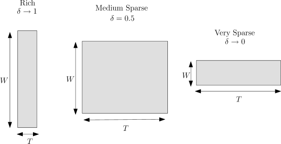
Figure 2: Optimal packet configurations with perfect receiver CSI and limited feedback as a function of richness of the channel. Three cases are illustrated here: Rich multipath $(\delta\rightarrow 1)$, medium sparsity $(\delta=0.5)$ and very high sparsity $(\delta\rightarrow 0)$.

IV Achievable Rates with Channel Estimation at the Receiver

In contrast to the perfect receiver CSI case, we now consider the more realistic case where no CSI is available a priori. We first consider only an average power constraint and show that the first-order term of the benchmark capacity can be achieved if the channel is sparse and the channel coherence dimension, $\mathnormal{N_{c}}$, scales with ${\sf{SNR}}$ at an appropriate rate, allowing the receiver to learn the channel reliably. We also show that this is infeasible when the channel is rich, due to poor channel estimation.

More specifically, the focus is here on a training-based signaling scheme where the transmitted signals include training symbols to enable channel estimation and coherent detection. The restriction to training schemes is motivated by their easy realizability. The total energy available for training and communication is $PT$, of which a fraction $\eta$ is used for training and the remaining fraction $(1-\eta)$ is used in communication. With the block fading model, this means that one signal space dimension in each coherence subspace is used for training and the remaining $\left(\mathnormal{N_{c}}-1\right)$ are used in communication. This is pictorially illustrated in Fig. 3. We consider minimum mean-squared error (MMSE) channel estimation and the reader is referred to [13, Sec. IIc] for more details on the training scheme.

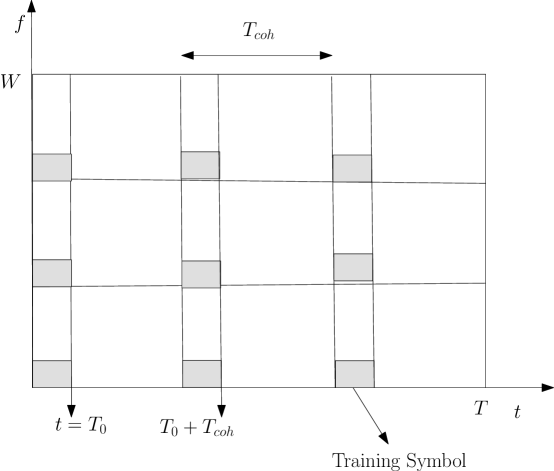
Figure 3: Training-based signaling scheme in the STF domain. The $D$ estimated channel coefficients determine the $D$ feedback bits for the communication scheme with limited feedback.

IV-A Achievable Rates under Average Power Constraint

Let $\widehat{C}_{{\sf train},1,{\sf LT}}({\sf{SNR}})$ denote the average mutual information achievable (per-dimension) with the causal training scheme under the average power constraint. We proceed along the same lines as the no feedback case [13, Lemma 1] to characterize $\widehat{C}_{{\sf train},1,{\sf LT}}({\sf{SNR}})$. Let $\mathbf{H}$ be the actual channel, $\widehat{\mathbf{H}}$ be the estimated channel and ${\bf\Delta}=\mathbf{H}-\widehat{\mathbf{H}}$ denote the estimation error matrix. We begin with the following well-known lower-bound [26] to $\widehat{C}_{{\sf train},1,{\sf LT}}({\sf{SNR}})$:

$$\widehat{C}_{{\sf train},1,{\sf LT}}({\sf{SNR}})\geq\sup_{\mathbf{Q}}\frac{{{\mathbf{E}}}\left[\textstyle{\log\det\textstyle{\big{(}{\mathbf{I}}_{(\mathnormal{N_{c}}-1)D}+\widehat{\mathbf{H}}{\mathbf{Q}}\widehat{\mathbf{H}}^{H}\left({\mathbf{I}}+\Sigma_{{\mathbf{\Delta}}{\mathbf{x}}}\right)^{-1}\big{)}}}\right]}{\mathnormal{N_{c}}D}$$ (58)

where the supremum is over $\{\mathbf{Q}:\hskip 1.4457pt{\rm Tr}(\mathbf{Q})\hskip 1.4457pt\leq\hskip 1.4457pt(1-\eta)TP\}$. The optimal $\mathbf{Q}$ is again diagonal and analogous to (23), equals

$$\mathbf{Q} = {\mathrm{diag}}\big{(}\underbrace{q_{1},\cdots,q_{1}}_{\mathnormal{N_{c}}-1}\hskip 1.4457pt,\hskip 1.4457pt\underbrace{q_{2},\cdots,q_{2}}_{\mathnormal{N_{c}}-1}\hskip 1.4457pt,\cdots,\hskip 1.4457pt\underbrace{q_{D},\cdots,q_{D}}_{\mathnormal{N_{c}}-1}\big{)}$$ (59)

$$q_{i} = \frac{(1-\eta)TP}{(\mathnormal{N_{c}}-1)D}\cdot\frac{\chi\left(|\widehat{h}_{i}|^{2}\geq{\sf h^{train}_{t}}\right)}{{\mathbf{E}}\left[\chi\left(|\widehat{h}|^{2}\geq{\sf h^{train}_{t}}\right)\right]}$$ (60)

where ${\sf h^{train}_{t}}$ is the threshold in the training case. The following theorem describes conditions under which the rates achievable with the training scheme converge to those in the coherent case.

Theorem 2

If $\mathnormal{N_{c}}=\frac{1}{{\sf{SNR}}^{\mu}}$ for some $\mu>1$, then

$$\lim_{{\sf{SNR}}\rightarrow 0}\frac{\widehat{C}_{{\sf train},1,{\sf LT}}({\sf{SNR}})}{\widehat{C}_{{\sf coh},1,{\sf LT}}({\sf{SNR}})}=1.$$ (61)

Proof:

Using the choice of $\mathbf{Q}$ from (60) in (58) and proceeding along the lines of (III-B), we obtain

$$\widehat{C}_{{\sf train},1,{\sf LT}}\left({\sf h^{train}_{t}},\eta,\mathnormal{N_{c}},{\sf{SNR}}\right) = \kappa_{1}\cdot\bigg{[}\log\left(1+\frac{(1-\eta)(1+\eta\mathnormal{N_{c}}{\sf{SNR}}){\sf h^{train}_{t}}{\sf{SNR}}}{(1-\eta){\sf{SNR}}+\kappa_{1}\kappa_{2}}\right)$$ (62)

$${\hskip 18.06749pt}+\nu_{\frac{(1-\eta)(1+\eta\mathnormal{N_{c}}{\sf{SNR}}){\sf h^{train}_{t}}{\sf{SNR}}+(1-\eta){\sf{SNR}}+\kappa_{1}\kappa_{2}}{\eta(1-\eta)\mathnormal{N_{c}}{\sf{SNR}}^{2}}}\bigg{]},$$

$$\kappa_{1} = e^{-\frac{{\sf h^{train}_{t}}(1+\eta\mathnormal{N_{c}}{\sf{SNR}})}{\eta\mathnormal{N_{c}}{\sf{SNR}}}},\>\>\kappa_{2}=\eta(\mathnormal{N_{c}}-1){\sf{SNR}}+\left(1-\frac{1}{\mathnormal{N_{c}}}\right)$$ (63)

where $\nu_{\bullet}$ is as defined following (39). The tightest lower bound to (62) is obtained by maximizing $\widehat{C}_{{\sf train},1,{\sf LT}}\left({\sf h^{train}_{t}},\eta,\mathnormal{N_{c}},{\sf{SNR}}\right)$ over $\eta$, the fraction of energy spent on training, and over ${\sf h^{train}_{t}}$:

$${C}^{*}_{{\sf train},1,{\sf LT}} = \max\limits_{{\sf h^{train}_{t}}}\left[\max\limits_{\eta}\widehat{C}_{{\sf train},1}\left({\sf h^{train}_{t}},\eta,\mathnormal{N_{c}},{\sf{SNR}}\right)\right].$$ (64)

Performing the optimization in (64) seems difficult. Motivated by our study in Sec. III, we now assume a specific form for the threshold: ${\sf h^{train}_{t}}=\epsilon\log\left(\frac{1}{{\sf{SNR}}}\right)$. It is shown in Appendix -C that with this choice of ${\sf h^{train}_{t}}$, the optimal choice for $\eta$ and $\mathnormal{N_{c}}$ can be obtained in closed form and the desired result in (61) is established.

Alternatively, we demonstrate a sub-optimal, but simpler approach that suffices to obtain (61). This approach uses the choice of $\eta$ that optimizes the average mutual information in the no feedback case [13, Lemma 2]. This choice, denoted by $\eta^{*}$, is given as

$$\eta^{*} = \textstyle{\frac{\mathnormal{N_{c}}{\sf{SNR}}+\mathnormal{N_{c}}-1}{(\mathnormal{N_{c}}-2)\mathnormal{N_{c}}{\sf{SNR}}}\cdot\left[\sqrt{1+\frac{\mathnormal{N_{c}}{\sf{SNR}}(\mathnormal{N_{c}}-2)}{\mathnormal{N_{c}}{\sf{SNR}}+\mathnormal{N_{c}}-1}}-1\right]}.$$ (65)

Let ${\sf h^{train,\hskip 1.4457pt\star}_{t}}=\frac{\eta^{*}\mathnormal{N_{c}}{\sf{SNR}}}{1+\eta^{*}\mathnormal{N_{c}}{\sf{SNR}}}{\sf h_{t}}$ where ${\sf h_{t}}\sim\lambda\log\left(\frac{1}{{\sf{SNR}}}\right)$, $\kappa_{1}^{\star}=\kappa_{1}|_{\eta^{*},\hskip 1.4457pt{\sf h^{train,\hskip 1.4457pt\star}_{t}}}$ and $\kappa_{2}^{\star}=\kappa_{2}|_{\eta^{*}}$. If we define,

$$A_{1} = \textstyle{\frac{(1-\eta^{*})(1+\eta^{*}\mathnormal{N_{c}}{\sf{SNR}})\hskip 1.4457pt{\sf h^{train,\hskip 1.4457pt\star}_{t}}{\sf{SNR}}}{(1-\eta^{*}){\sf{SNR}}+\kappa_{1}^{\star}\kappa_{2}^{\star}}},$$ (66)

$$A_{2} = \textstyle{\frac{(1-\eta^{*})(1+\eta^{*}\mathnormal{N_{c}}{\sf{SNR}})\hskip 1.4457pt{\sf h^{train,\hskip 1.4457pt\star}_{t}}{\sf{SNR}}+(1-\eta^{*}){\sf{SNR}}+\kappa_{1}^{\star}\kappa_{2}^{\star}}{\eta^{*}(1-\eta^{*})\mathnormal{N_{c}}{\sf{SNR}}^{2}}},$$ (67)

it is cumbersome, but straightforward to show that

$$\lim\limits_{{\sf{SNR}}\rightarrow 0}A_{1}=0\hskip 3.61371pt\hskip 3.61371pt{\rm and}\hskip 3.61371pt\hskip 3.61371pt\lim\limits_{{\sf{SNR}}\rightarrow 0}\frac{1}{A_{2}}=0$$ (68)

for any $\mu>0$. From (62), we then have

$$\max\limits_{{\sf h^{train}_{t}},\eta}\widehat{C}_{{\sf train},1,{\sf LT}}({\sf h^{train}_{t}},\eta,\mathnormal{N_{c}},{\sf{SNR}}) \geq \widehat{C}_{{\sf train},1,{\sf LT}}({\sf h^{train,\hskip 1.4457pt\star}_{t}},\eta^{*},\mathnormal{N_{c}},{\sf{SNR}})$$ (69)

$$= \kappa_{1}\cdot\left[\log\left(1+A_{1}\right)+\nu_{A_{2}}\right]$$ (70)

$$\stackrel{{\scriptstyle(a)}}{{\geq}} \kappa_{1}\cdot\left[\log\left(1+A_{1}\right)+\frac{1}{2}\log\left(1+\frac{2}{A_{2}}\right)\right]$$ (71)

$$\stackrel{{\scriptstyle(b)}}{{\approx}} \kappa_{1}\cdot\left[A_{1}+\frac{1}{A_{2}}\right]$$ (72)

where (a) follows from (40) and (b) is the low-${\sf{SNR}}$ approximation to (71). Substituting for ${\sf h^{train,\hskip 1.4457pt\star}_{t}}$ and simplifying we can reduce the lower bound in (72) to

$$\widehat{C}_{{\sf train},1,{\sf LT}}({\sf{SNR}})\geq(1-\eta^{*})\left(\frac{\mathnormal{N_{c}}}{\mathnormal{N_{c}}-1}\right)\left(\frac{\eta^{*}\mathnormal{N_{c}}{\sf{SNR}}}{1+\eta^{*}\mathnormal{N_{c}}{\sf{SNR}}}\right)\left[1+{\sf h_{t}}\right]{\sf{SNR}}.$$ (73)

Substituting for $\eta^{*}$ from (65) and $\mathnormal{N_{c}}=\frac{1}{{\sf{SNR}}^{\mu}}$, it can be checked that when $\mu>1$ the leading term is $\left[1+{\sf h_{t}}\right]{\sf{SNR}}$ which equals the first-order term of the coherent capacity as described by Corollary 1. On the other hand when $\mu<1$, the leading term takes the form ${\mathcal{O}}\left({\sf{SNR}}^{\frac{3-\mu}{2}}\right)$ and hence, $\mu>1$ is necessary. ∎

Having established the result with an average power constraint, let us consider the instantaneous power constraint case.

IV-B Achievable Rates under Instantaneous Power Constraint

We impose a constraint as in (45) for the communication phase of the training scheme. With the same power allocation scheme as in (47) (Sec. III-B), we obtain

$$\widehat{C}_{{\sf train},1,{\sf ST}}({\sf{SNR}}) = \left(1-\frac{1}{\mathnormal{N_{c}}}\right)\frac{1}{D}\hskip 1.4457pt\sum_{i=1}^{D}{\mathbf{E}}\left[\log\left(1+\frac{|\widehat{h}_{i}|^{2}q_{i}(1+E_{tr})}{1+q_{i}+E_{tr}}{\hskip 7.22743pt}\times\right.\right.$$ (74)

$$\left.\left.\chi\left(\sum_{j=1}^{i}\chi(|\widehat{h}_{j}|^{2}\geq{\sf h^{train}_{t}})\leq\frac{ADe^{-\frac{{\sf h^{train}_{t}}(1+\eta\mathnormal{N_{c}}{\sf{SNR}})}{\eta\mathnormal{N_{c}}{\sf{SNR}}}}}{(1-\eta)}\right)\right)\right]$$

$$= \widehat{C}_{{\sf train},1,{\sf LT}}({\sf{SNR}})\cdot\frac{\sum_{i=1}^{D}p^{{\sf train}}_{i}}{D}$$ (75)

where $E_{tr}=\eta\mathnormal{N_{c}}\hskip 1.4457pt{\sf{SNR}}$ and $p^{{\sf train}}_{i}={\mathrm{Pr}}\left(\sum\limits_{j=1}^{i}\chi(|\widehat{h}_{j}|^{2}\geq{\sf h^{train}_{t}})\leq\frac{ADe^{-\frac{{\sf h^{train}_{t}}(1+\eta\mathnormal{N_{c}}{\sf{SNR}})}{\eta\mathnormal{N_{c}}{\sf{SNR}}}}}{(1-\eta)}\right)$. Understanding when $\frac{\sum_{i=1}^{D}p^{{\sf train}}_{i}}{D}\rightarrow 1$ is similar to the case studied in Sec. III-B. Taking recourse to the analysis of Prop. 1 by using a threshold of the form ${\sf h^{train,\hskip 1.4457pt\star}_{t}}=\frac{\eta^{*}\mathnormal{N_{c}}{\sf{SNR}}}{1+\eta^{*}\mathnormal{N_{c}}{\sf{SNR}}}{\sf h_{t}}$ where $\eta^{*}$ is as in (65) and ${\sf h_{t}}\sim\lambda\log\left(\frac{1}{{\sf{SNR}}}\right)$, it can be shown that the $\frac{\sum_{i=1}^{D}p^{{\sf train}}_{i}}{D}$ is lower bounded by the same expression as in (49) and (50) with $A$ replaced by $\frac{A}{1-\eta^{*}}$. After some simplifications, we can conclude that if $\frac{{\mathbf{E}}\left[{\sf D}_{\sf eff}\right]}{1-\eta^{*}}-{\sf h_{t}}\rightarrow\infty$, then $\widehat{C}_{{\sf train},1,{\sf ST}}({\sf{SNR}})\rightarrow\widehat{C}_{{\sf train},1,{\sf LT}}({\sf{SNR}})$. Note that the condition in the perfect CSI case is more stringent than in the training setting. That is, if the channel is such that ${\mathbf{E}}\left[{\sf D}_{\sf eff}\right]-{\sf h_{t}}\rightarrow\infty$, then it automatically ensures that $\frac{{\mathbf{E}}\left[{\sf D}_{\sf eff}\right]}{1-\eta^{*}}-{\sf h_{t}}\rightarrow\infty$.

IV-C Discussion

The analysis in Sec. IV-A and IV-B reveals that the following conditions are critical:

1. The channel coherence dimension, $\mathnormal{N_{c}}$, scales with ${\sf{SNR}}$ according to $\mathnormal{N_{c}}\sim\frac{1}{{\sf{SNR}}^{\mu}}$, $\mu>1$, and

2. The independent degrees of freedom (DoF), $D$, in the channel scales with ${\sf{SNR}}$ such that $\frac{{\mathbf{E}}\left[{\sf D}_{\sf eff}\right]}{1-\eta^{*}}-{\sf h_{t}}=\frac{D\hskip 1.4457pte^{{\sf h_{t}}}}{1-\eta^{*}}-{\sf h_{t}}\rightarrow\infty$ as ${\sf{SNR}}\rightarrow 0$.

With only an average power constraint, C1 is necessary and sufficient so that $\widehat{C}_{{\sf train},1,{\sf LT}}({\sf{SNR}})\rightarrow\widehat{C}_{{\sf coh},1,{\sf LT}}({\sf{SNR}})$. In particular, with $\lambda\rightarrow 1$, we approach the perfect CSI benchmark. When there is an instantaneous power constraint, we need to satisfy both C1 and C2 so that the benchmark can be attained.

We now study the implications of these conditions. Note that C1 predicates a certain minimum channel coherence level to ensure the fidelity of the training performance. That is, the larger the value of $\mu$ and hence, $\mathnormal{N_{c}}$, the more easier it is to meet the benchmark. On the other hand, C2 describes the required growth rate in the DoF, $D$, so that ${\mathbf{E}}\left[{\sf D}_{\sf eff}\right]-{\sf h_{t}}\rightarrow\infty$ and the instantaneous power constraint is satisfied without any rate loss. That is, the larger the value of $D$, the more easier it is to meet the benchmark. It is clear that the two conditions are somewhat conflicting in nature since for a richer channel, it is easier to increase $D$ but more difficult to increase $\mathnormal{N_{c}}$, while for a sparser channel, it is the reverse. Therefore a natural question is if they can be satisfied simultaneously.

To understand this, we first study the achievability of C1. What are the conditions on the channel parameters ($T_{m}$, $W_{d}$, $\delta_{1}$ and $\delta_{2}$) and how do they interact with the signal space parameters ($T$, $W$ and $P$) so that $\mu>1$ is feasible? As we discuss next, by leveraging delay and Doppler sparsities and using peaky signaling (when necessary), $\mu>1$ is achievable.

B1) Rich multipath: When the channel is rich in both delay and Doppler, $\mathnormal{N_{c}}=\frac{1}{T_{m}W_{d}}$ is fixed and does not scale with ${\sf{SNR}}$. Thus we can never maintain the scaling relationship in $\mathnormal{N_{c}}$ as in Theorem 2 and C1 can never be satisfied. Therefore, we cannot attain the benchmark even under an average power constraint.

B2) Doppler sparsity only: In this case $\mathnormal{W_{coh}}=\frac{1}{T_{m}}$ is fixed and the scaling in $\mathnormal{N_{c}}$ is only through $\mathnormal{T_{coh}}\sim f_{2}(T)$ (see (15)). Therefore, by scaling $T$ with $W$ according to $T\sim f_{2}^{-1}\left(W^{\mu}\right)$ and choosing $\mu>1$, we have $\mathnormal{N_{c}}\sim\mathnormal{T_{coh}}\sim f_{2}\left(f_{2}^{-1}(W^{\mu})\right)\sim\frac{1}{{\sf{SNR}}^{\mu}}$. For the power-law scaling in (16), we obtain

$$T\sim W^{\frac{\mu}{1-\delta_{1}}}.$$ (76)

Note that as $\delta_{1}$ increases and the channel gets more richer, $T$ increases monotonically in (76).

B3) Delay sparsity only: In this case, $\mathnormal{T_{coh}}=\frac{1}{W_{d}}$ and $\mathnormal{N_{c}}=\mathnormal{W_{coh}}\mathnormal{T_{coh}}$ scales with ${\sf{SNR}}$ only through $\mathnormal{W_{coh}}\sim f_{1}\left(\frac{1}{{\sf{SNR}}}\right)$. Therefore, for any sub-linear function $f_{1}(\cdot)$, we cannot satisfy $\mu>1$. A possible solution to overcome this difficulty is to use peaky signaling where training and communication are performed only on a subset of the $D$ coherence subspaces. Modeling peakiness as in [4, 13] and defining $\zeta={\sf{SNR}}^{\gamma},\hskip 3.61371pt\gamma>0$ as the fraction of $D$ over which signaling is performed, it can be shown that [13, Lemma 3] the condition for asymptotic coherence gets relaxed to $\mathnormal{N_{c}}=\frac{1}{{\sf{SNR}}^{\mu_{{\mathrm{peaky}}}}}$ from the original $\mathnormal{N_{c}}=\frac{1}{{\sf{SNR}}^{\mu}}$ where $\mu_{{\mathrm{peaky}}}=\mu+\gamma$. We require $\mu_{{\mathrm{peaky}}}>1$ which is the same as $\mu>1-\gamma$. For the power-law scaling in (16), we have $\mathnormal{N_{c}}\sim f_{1}(W)\sim W^{1-\delta_{2}}\sim\frac{1}{{\sf{SNR}}^{1-\delta_{2}}}$. Thus, if the peakiness coefficient $\gamma$ satisfies $\gamma>\delta_{2}$, we can satisfy the desired condition.

B4) Delay and Doppler sparsity: Using (15), we have $\mathnormal{W_{coh}}\sim f_{1}(W)$ and $\mathnormal{T_{coh}}\sim f_{2}(T)$. Therefore, if we scale $T$ with $W$ according to

$$T\sim f_{3}(W)\hskip 3.61371pt\hskip 3.61371pt\hskip 3.61371pt\text{with}\hskip 3.61371pt\hskip 3.61371pt\hskip 3.61371ptf_{3}(x)=f_{2}^{-1}\left(\frac{x^{\mu}}{f_{1}(x)}\right),$$ (77)

we have $\mathnormal{N_{c}}=\mathnormal{W_{coh}}\mathnormal{T_{coh}}\sim f_{1}(W)f_{2}(f_{3}(W))=f_{1}(W)f_{2}\left(f_{2}^{-1}\left(\frac{W^{\mu}}{f_{1}(W)}\right)\right)\sim\frac{1}{{\sf{SNR}}^{\mu}}$. Thus with $\mu>1$ in (77), we attain the desired scaling of $\mathnormal{N_{c}}$ with ${\sf{SNR}}$. For the power-law scaling in (16), the desired scaling in $\mathnormal{N_{c}}$ can be obtained by choosing $T$, $W$ and $P$ according to the following canonical relationship that is obtained using (16) in (77)

$$T=\frac{\left(T_{m}^{\delta_{2}}W_{d}^{\delta_{1}}\right)^{\frac{1}{1-\delta_{1}}}W^{\frac{\mu-1+\delta_{2}}{1-\delta_{1}}}}{P^{\frac{\mu}{1-\delta_{1}}}}.$$ (78)

From the above discussion, it is clear that channel sparsity is necessary and in addition we also require a specific scaling relationship between $T$ and $W$ as defined in (78). But this is necessary for achieving the benchmark capacity with an average power constraint (satisfying C1). We now study how this scaling law impacts the scaling of $D$ with ${\sf{SNR}}$, as in the instantaneous power case. This is critical in determining the achievability of C2, which we discuss next. We recall that by definition

$$D=\frac{TW}{\mathnormal{N_{c}}}=TW\>{\sf{SNR}}^{\mu}.$$ (79)

Using (78) in (79) and simplifying, we obtain the induced scaling behavior on $D$ with ${\sf{SNR}}$ as

$$D\sim{\sf{SNR}}^{\frac{\delta_{1}\left(1-\mu\right)-\delta_{2}}{1-\delta_{1}}}.$$ (80)

Therefore, we have ${\mathbf{E}}\left[{\sf D}_{\sf eff}\right]-{\sf h_{t}}={\sf{SNR}}^{\lambda+\frac{\delta_{1}\left(1-\mu\right)-\delta_{2}}{1-\delta_{1}}}+\lambda\log({\sf{SNR}})$ and consequently

$${\mathbf{E}}\left[{\sf D}_{\sf eff}\right]-{\sf h_{t}}\rightarrow\begin{cases}\infty&{\rm if}\hskip 3.61371pt0<\lambda<\frac{\delta_{2}+\left(\mu-1\right)\delta_{1}}{1-\delta_{1}}\\ -\infty&{\rm if}\hskip 3.61371pt1>\lambda\geq\frac{\delta_{2}+\left(\mu-1\right)\delta_{1}}{1-\delta_{1}}.\end{cases}$$ (81)

It is easily seen that

$$\frac{\delta_{2}+\left(\mu-1\right)\delta_{1}}{1-\delta_{1}}>1\Longleftrightarrow\mu>\frac{1-\delta_{2}}{\delta_{1}}$$ (82)

which yields ${\mathbf{E}}\left[{\sf D}_{\sf eff}\right]-{\sf h_{t}}\rightarrow\infty$ for all $\lambda\in(0,1)$, and C2 is satisfied as desired. The special cases of delay sparsity only and Doppler sparsity only (as in B2 and B3) are simple extensions and follow naturally.

To summarize,

$$\mu>1 \Longrightarrow$$ C1 is achievable (83)

$$\mu>\frac{1-\delta_{2}}{\delta_{1}} \Longrightarrow \textbf{C2 is achievable}.$$ (84)

Therefore,

$$\mu>\max\left(1,\frac{1-\delta_{2}}{\delta_{1}}\right)\Longrightarrow\textbf{C1 and C2 are achievable}.$$ (85)

We now elucidate the optimal packet configurations for different levels of channel sparsity. Analogous to the discussion in Sec. III-D, we focus on the power-law scaling and illustrate rules of thumb for choosing $T$ and $W$ for a given $N=TW$. Assuming symmetrical sparsity $(\delta_{1}=\delta_{2}=\delta)$, we note the following two cases:

$$\textbf{Case 1:}\>\>\frac{1-\delta}{\delta}>1\Longleftrightarrow\delta<0.5,\hskip 3.61371pt\hskip 3.61371pt\hskip 3.61371ptT\sim W^{\rho},\hskip 3.61371pt\rho>\frac{1-\delta}{\delta}$$ (86)

$$\textbf{Case 2:}\>\>\frac{1-\delta}{\delta}<1\Longleftrightarrow\delta>0.5,\hskip 3.61371pt\hskip 3.61371pt\hskip 3.61371ptT\sim W^{\rho},\hskip 3.61371pt\rho>\frac{\delta}{1-\delta}.$$ (87)

The corresponding packet configurations are shown in Fig. 4 for $\delta\rightarrow 0$, $\delta=0.5$ and $\delta\rightarrow 1$. It is observed that the slowest scaling in $T$ with $W$ is obtained for $\delta=0.5$ when the DoF follow a square-root scaling law with signal space dimension. On either extreme of this square-root law, the required scaling in $T$ with $W$ only gets worse. This conclusion is expected and is consistent with the contradictory requirements presented by C1 and C2. When $\delta<0.5$, the channel conditions are more favorable towards scaling $\mathnormal{N_{c}}$ as a function of ${\sf{SNR}}$ (specified by C1). However, the required scaling of $D$ with ${\sf{SNR}}$ (specified by C2) is non-trivial and ultimately dominates the required scaling of $T$ with $W$. On the other hand, when $\delta>0.5$, the relatively less sparse channel conditions are favorably disposed towards the scaling of $D$ as a function of ${\sf{SNR}}$, but this is at the cost of scaling in $\mathnormal{N_{c}}$. For the case of asymmetrically sparse channels, it can be shown that this desirable condition (slowest scaling of $T$ with $W$) generalizes to $\delta_{1}+\delta_{2}=1$.

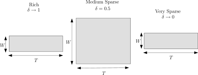
Figure 4: Optimal packet configurations in the non-coherent scenario with limited feedback. Three cases illustrated here are rich multipath $(\delta\rightarrow 1)$, medium sparsity $(\delta=0.5)$ and very high sparsity $(\delta\rightarrow 0)$.

V Concluding Remarks

In this paper, we studied the achievable rates of sparse multipath channels with limited feedback. The focus of our analysis is in the wideband$/$low-${\sf{SNR}}$ regime. Our investigation includes constraining both the average and the instantaneous transmit powers. We first analyzed the case when the receiver has perfect CSI and when one bit (per channel coefficient) of this CSI is known perfectly at the transmitter. We established conditions under which the rates achievable with this scheme approach the capacity with perfect receiver and transmitter CSI. For sparse channels, these conditions translate to certain optimal packet configurations for signaling. When the receiver has no CSI a priori, we studied the performance of a training scheme. It is shown that with only an average power constraint, channel sparsity is necessary to attain the coherent performance. With an instataneous power constraint, we established conditions on optimal packet configurations in order to approach the benchmark capacity gain asymptotically as ${\sf{SNR}}\rightarrow 0$.

TABLE I: Conditions necessary to achieve the perfect CSI benchmark of $\log\left(\frac{1}{{\sf{SNR}}}\right){\sf{SNR}}$.

CSI	CSI	Power	Necessary	Signaling
Rx.	Tx.	Const.	Conditions	Parameters
Perf.	Perf.	-	$h_{w}\sim\log\left(\frac{1}{{\sf{SNR}}}\right)$	Waterfilling; see [2, 17]
Perf.	$1$ bit	Avg.	${\sf h_{t}}=\lambda\log\left(\frac{1}{{\sf{SNR}}}\right),\hskip 3.61371pt\lambda\rightarrow 1$	No constraints on richness or $T$, $W$;
				see [2, 17, 18]
Perf.	$1$ bit	Inst.	${\sf h_{t}}=\lambda\log\left(\frac{1}{{\sf{SNR}}}\right)$	Rich channel: no constraint on $T$ or $W$,
			for $\lambda<1$, and	Sparse ($T$ fixed): $\lambda<\delta_{2}$ limits rates,
			${\mathbf{E}}\left[{\sf D}_{\sf eff}\right]-{\sf h_{t}}\rightarrow\infty$	Sparse (general): $T\sim W^{\rho}$,   $\rho\geq\frac{1-\delta_{2}}{\delta_{1}}$
Train.	$1$ bit	Avg.	$\mathnormal{N_{c}}\sim\frac{1}{{\sf{SNR}}^{\mu}},\hskip 3.61371pt\mu>1$	Rich channel: Impossible,
				Sparsity (Doppler): Non-peaky
				scheme with $T\sim W^{\frac{\mu}{1-\delta_{1}}}$,
				Sparsity (delay): Peaky scheme with
				peakiness coefficient $\gamma>\delta_{2}$,
				Sparsity (both): Non-peaky scheme;
				see (77) and (78)
Train.	$1$ bit	Inst.	$\mathnormal{N_{c}}\sim\frac{1}{{\sf{SNR}}^{\mu}},\hskip 3.61371pt\mu>1$	Rich channel: Impossible,
			and $\frac{{\mathbf{E}}\left[{\sf D}_{\sf eff}\right]}{1-\eta^{*}}-{\sf h_{t}}\rightarrow\infty$	Sparse (both): $\mu>\frac{1-\delta_{2}}{\delta_{1}}$ for no rate
				loss, else $\lambda<\frac{\delta_{2}+(\mu-1)\delta_{1}}{1-\delta_{1}}$

We contrast the results of this work with recent observations in [17, 18]. The focus in [17, 18] is on training schemes and on scenarios where $\mathnormal{T_{coh}}$ increases as ${\sf{SNR}}$ decreases, although there is no mention of how such a scaling law can be realized in practice. In particular, the authors show that capacity scales as $\log\left(\mathnormal{T_{coh}}\right){\sf{SNR}}$ if $\log(\mathnormal{T_{coh}})\preceq\log\left(\frac{1}{{\sf{SNR}}}\right)$ and equals the coherent capacity, $\log\left(\frac{1}{{\sf{SNR}}}\right){\sf{SNR}}$, when $\log(\mathnormal{T_{coh}})\succeq\log\left(\frac{1}{{\sf{SNR}}}\right)$. On the other hand, we have shown that when the channel is sparse, channel coherence scales naturally with $T$ and $W$ and the benchmark gain, $\log\left(\frac{1}{{\sf{SNR}}}\right)$, can always be achieved by appropriately choosing $T$ and $W$. Furthermore, while [17, 18] considered only an average power constraint, we have established achievability under both average and instantaneous power constraints. Also, peaky training schemes are necessary in the framework of [17] to achieve perfect training performance. Such schemes would violate any finite instantaneous power constraint. Our findings here reveal that channel sparsity is a degree of freedom that can be exploited to obtain near-coherent performance with non-peaky training schemes. Table I provides a short summary of our contributions and places them in the context of [2, 17, 18].

Finally, we note that the results obtained here closely parallel our earlier work [13] where we studied the achievable rates with training and no feedback. We showed that when $\mathnormal{N_{c}}=\frac{1}{{\sf{SNR}}^{\mu}}$ with $\mu>1$, the channel is asymptotically coherent; channel estimation performance is near-perfect at a vanishing energy cost. Analogous to [13], we have shown here that under the assumption of an error-free $D$-bit feedback link, the rate achievable with the training scheme converges to the perfect CSI benchmark. Furthermore, the cost of feedback, measured in terms of the number of feedback bits per dimension $(D/N)$ converges asymptotically to zero in a sparse channel.

-A Tightness of $\widehat{C}_{{\sf coh},1,{\sf LT}}({\sf{SNR}})$ to $C_{{\sf coh},1,{\sf LT}}({\sf{SNR}})$ as ${\sf{SNR}}\rightarrow 0$

Let $\chi_{i}$ denote the random variable $\chi(|h_{i}|^{2}\geq{\sf h_{t}})$. Defining $\gamma\triangleq\frac{\left|C_{{\sf coh},1,{\sf LT}}({\sf{SNR}})-\widehat{C}_{{\sf coh},1,{\sf LT}}({\sf{SNR}})\right|}{C_{{\sf coh},1,{\sf LT}}({\sf{SNR}})}$, we have

$$\gamma = \frac{1}{D}\left|\sum_{i=1}^{D}{\mathbf{E}}\left[\log\left(1+\frac{\frac{TP|h_{i}|^{2}\chi_{i}(De^{-{\sf h_{t}}}-\sum_{i}\chi_{i})}{\sum_{i}\chi_{i}N_{c}De^{-{\sf h_{t}}}}}{1+\frac{TP|h_{i}|^{2}\chi_{i}}{N_{c}De^{-{\sf h_{t}}}}}\right)\right]\right|$$ (88)

$$\leq \frac{1}{D}\sum_{i=1}^{D}{\mathbf{E}}\left|\log\left(1+\frac{\frac{TP|h_{i}|^{2}\chi_{i}(De^{-{\sf h_{t}}}-\sum_{i}\chi_{i})}{\sum_{i}\chi_{i}N_{c}De^{-{\sf h_{t}}}}}{1+\frac{TP|h_{i}|^{2}\chi_{i}}{N_{c}De^{-{\sf h_{t}}}}}\right)\right|$$ (89)

$$\stackrel{{\scriptstyle(a)}}{{\leq}} \frac{1}{D}\sum_{i=1}^{D}{\mathbf{E}}\left|\frac{\frac{TP|h_{i}|^{2}\chi_{i}(De^{-{\sf h_{t}}}-\sum_{i}\chi_{i})}{\sum_{i}\chi_{i}N_{c}De^{-{\sf h_{t}}}}}{1+\frac{TP|h_{i}|^{2}\chi_{i}}{N_{c}De^{-{\sf h_{t}}}}}\right|$$ (90)

$$= \frac{TP}{N_{c}D^{2}e^{-{\sf h_{t}}}}\sum_{i=1}^{D}{\mathbf{E}}\left[\frac{|h_{i}|^{2}\chi_{i}\left|De^{-{\sf h_{t}}}-\sum_{i}\chi_{i}\right|}{\sum_{i}\chi_{i}\left(1+\frac{TP|h_{i}|^{2}\chi_{i}}{N_{c}De^{-{\sf h_{t}}}}\right)}\right]$$ (91)

$$\stackrel{{\scriptstyle(b)}}{{=}} \frac{TP}{N_{c}De^{-{\sf h_{t}}}}{\mathbf{E}}\left[\frac{|h_{1}|^{2}\chi_{1}\left|De^{-{\sf h_{t}}}-\sum_{i}\chi_{i}\right|}{\sum_{i}\chi_{i}\left(1+\frac{TP|h_{1}|^{2}\chi_{1}}{N_{c}De^{-{\sf h_{t}}}}\right)}\right]\triangleq\gamma_{0}$$ (92)

where (a) follows from the log-inequality and (b) from the fact that $\{h_{i}\}$ are i.i.d. Conditioning on $\chi_{1}$, we now have

$$\gamma_{0} = \frac{TP}{N_{c}De^{-{\sf h_{t}}}}{\mathbf{E}}[\chi_{1}]\hskip 1.4457pt{\mathbf{E}}_{h_{1},\{\chi_{j},j>1\}}\left[\frac{|h_{1}|^{2}\left|De^{-{\sf h_{t}}}-(1+\sum_{j>1}\chi_{j})\right|}{(1+\sum_{j>1}\chi_{j})\left(1+\frac{TP|h_{1}|^{2}}{N_{c}De^{-{\sf h_{t}}}}\right)}\right]$$ (93)

$$= {\sf{SNR}}\cdot{\mathbf{E}}_{h_{1},\{\chi_{j},j>1\}}\left[\frac{|h_{1}|^{2}\left|De^{-{\sf h_{t}}}-(1+\sum_{j>1}\chi_{j})\right|}{(1+\sum_{j>1}\chi_{j})\left(1+\frac{TP|h_{1}|^{2}}{N_{c}De^{-{\sf h_{t}}}}\right)}\right]$$ (94)

$$\stackrel{{\scriptstyle(a)}}{{=}} {\sf{SNR}}\cdot{\mathbf{E}}_{h_{1}}\left[\frac{|h_{1}|^{2}}{1+\frac{TP|h_{1}|^{2}}{N_{c}De^{-{\sf h_{t}}}}}\right]\cdot{\mathbf{E}}_{\{\chi_{j},j>1\}}\left[\frac{\left|De^{-{\sf h_{t}}}-(1+\sum_{j>1}\chi_{j})\right|}{(1+\sum_{j>1}\chi_{j})}\right]$$ (95)

$$\leq {\sf{SNR}}\cdot{\mathbf{E}}[|h_{1}|^{2}]\cdot{\mathbf{E}}_{\{\chi_{j},j>1\}}\left[\frac{\left|De^{-{\sf h_{t}}}-(1+\sum_{j>1}\chi_{j})\right|}{(1+\sum_{j>1}\chi_{j})}\right]\triangleq\gamma_{1}$$ (96)

where (a) follows from the fact that $h_{1}$ and $\{\chi_{j},j>1\}$ are independent.

To show the closeness of $\widehat{C}_{{\sf coh},1,{\sf LT}}({\sf{SNR}})$ to $C_{{\sf coh},1,{\sf LT}}({\sf{SNR}})$, we now produce an upper bound for $\gamma_{1}$ that tends to $0$ as ${\sf{SNR}}\rightarrow 0$. Our goal is to show that given any choice of $D$, $\frac{\gamma_{1}}{{\sf{SNR}}}$ is bounded. Consider

$${\mathbf{E}}_{\{\chi_{j},j>1\}}\left[\frac{\left|De^{-{\sf h_{t}}}-(1+\sum_{j>1}\chi_{j})\right|}{(1+\sum_{j>1}\chi_{j})}\right] = {\mathbf{E}}_{\{\chi_{j},j>1\}}\left[\left|\frac{De^{-{\sf h_{t}}}}{(1+\sum_{j>1}\chi_{j})}-1\right|\right]$$

$$\stackrel{{\scriptstyle(a)}}{{\leq}} \underbrace{\sqrt{{\mathbf{E}}_{\chi_{j}}\left[\left(\frac{De^{-{\sf h_{t}}}}{(1+\sum_{j>1}\chi_{j})}\right)^{2}+1-2\frac{De^{-{\sf h_{t}}}}{(1+\sum_{j>1}\chi_{j})}\right]}}_{\triangleq\gamma_{2}}$$

where (a) is a consequence of Cauchy-Schwarz inequality. Let ${\sf E}$ denote $e^{-{\sf h_{t}}}$. We then have

$$\gamma_{2}\stackrel{{\scriptstyle(b)}}{{\leq}}\sqrt{1+D^{2}{\sf E}^{2}\cdot{\mathbf{E}}_{\chi_{j}}\left[\frac{1}{(1+\sum_{j>1}\chi_{j})^{2}}\right]-\frac{2D{\sf E}}{1+(D-1){\sf E}}}$$ (97)

where in (b) we have used the fact that ${\mathbf{E}}\left[\frac{1}{{\bf X}}\right]\geq\frac{1}{{\mathbf{E}}[{\bf X}]}$ for a positive random variable ${\bf X}$. We now estimate $\alpha\triangleq{\mathbf{E}}_{\chi_{j}}\left[\frac{1}{(1+\sum_{j>1}\chi_{j})^{2}}\right]$. It is easy to check that

$$\alpha=\sum_{i=0}^{D-1}{D-1\choose i}\frac{{\sf E}^{i}(1-{\sf E})^{D-1-i}}{(i+1)^{2}}.$$ (98)

Noting that

$$(1+y)^{D-1}=\sum_{i=0}^{D-1}{D-1\choose i}\hskip 3.61371pty^{i}$$ (99)

and integrating twice both sides of (99) with respect to $y$, we have

$$\frac{(1+y)^{D+1}}{D(D+1)}=\sum_{i=0}^{D-1}{D-1\choose i}\hskip 3.61371pt\frac{y^{i+2}}{(i+1)(i+2)}.$$ (100)

Using $y=\frac{{\sf E}}{1-{\sf E}}$ in (100), we have

$$\frac{1}{D(D+1){\sf E}^{2}}=\sum_{i=0}^{D-1}{D-1\choose i}\frac{{\sf E}^{i}(1-{\sf E})^{D-1-i}}{(i+1)(i+2)}.$$ (101)

Observe that $\frac{1}{(i+1)^{2}}\leq\frac{2}{(i+1)(i+2)}$ for all $i\geq 0$ and an upper bound for $\gamma_{2}$ is

$$\gamma_{2}\leq\sqrt{1+\frac{2D^{2}{\sf E}^{2}}{D(D+1){\sf E}^{2}}-\frac{2D{\sf E}}{1+(D-1){\sf E}}}=\sqrt{\frac{D^{2}{\sf E}-4D{\sf E}+3D-{\sf E}+1}{(D+1)(D{\sf E}-{\sf E}+1)}}$$ (102)

which is bounded for any choice of $D$. (In fact, the upper bound converges to $1$ as $D\rightarrow\infty$). Note that the bound in (102) is loose and one might expect that $\frac{\gamma_{1}}{{\sf{SNR}}}\rightarrow 0$ as $D\rightarrow\infty$ as a consequence of the law of large numbers. However, for our purpose, the proposed loose upper bound in (102) is sufficient.

-B Proof of Proposition 1

To compute $p_{i}\triangleq{\mathrm{Pr}}\left(\sum_{j=1}^{i}\chi(|h_{j}|^{2}\geq{\sf h_{t}})\leq ADe^{-{\sf h_{t}}}\right)$, we need the following result [27, Theorem 2.8, p. 57] on the tail probability of a sum of independent random variables.

Lemma 1

Let ${\bf X}_{i},i=1,\cdots,n$ be independent random variables with ${\mathbf{E}}[{\bf X}_{i}]=0$ and ${\mathbf{E}}[{\bf X}_{i}^{2}]=\sigma_{i}^{2}$. Define $B_{n}=\sum_{i=1}^{n}\sigma_{i}^{2}$. If there exists a positive constant $H$ such that

$${\mathbf{E}}[{\bf X}_{i}^{m}]\leq\frac{1}{2}m!\sigma_{i}^{2}H^{m-2}$$ (103)

for all $i$ and $x\geq\frac{B_{n}}{H}$, then we have ${\mathrm{Pr}}\big{(}\sum_{i=1}^{n}{\bf X}_{i}>x\big{)}\leq\exp\big{(}-\frac{x}{4H}\big{)}$. If $x\leq\frac{B_{n}}{H}$, then we have ${\mathrm{Pr}}\big{(}\sum_{i=1}^{n}{\bf X}_{i}>x\big{)}\leq\exp\big{(}-\frac{x^{2}}{4B_{n}}\big{)}$.

To apply Lemma 1, we set $n=i$ and ${\bf X}_{j}=\chi(|h_{j}|^{2}\geq{\sf h_{t}})-{\mathbf{E}}\left[\chi(|h_{j}|^{2}\geq{\sf h_{t}})\right]=\chi(|h_{j}|^{2}\geq{\sf h_{t}})-e^{-{\sf h_{t}}}=\chi_{j}-{\sf E}$ for $j=1,\cdots,i$. Then, a simple computation of the higher moments of ${\bf X}_{j}$ implies that ${\mathbf{E}}[{\bf X}_{j}^{2}]=\sigma_{j}^{2}={\sf E}(1-{\sf E})$, $B_{i}=i{\sf E}(1-{\sf E})$, ${\mathbf{E}}[{\bf X}_{j}^{m}]={\sf E}(1-{\sf E})\cdot((1-{\sf E})^{m-1}+(-1)^{m}{\sf E}^{m-1})$. It can be checked that $H=(1-{\sf E})$ is sufficient to satisfy the conditions of Lemma 1. With this setting, we have

$${\mathrm{Pr}}\left(\sum_{j=1}^{i}\chi(|h_{j}|^{2}\geq{\sf h_{t}})-i{\sf E}>(AD-i){\sf E}\right)\leq\left\{\begin{array}[]{cc}\exp\left(-\frac{(AD-i){\sf E}}{4(1-{\sf E})}\right)&{\rm if}\hskip 3.61371pti\leq\lfloor\frac{AD}{2}\rfloor,\\ \exp\left(-\frac{(AD-i)^{2}{\sf E}}{4i(1-{\sf E})}\right)&{\rm if}\hskip 3.61371pti\geq\lfloor\frac{AD}{2}\rfloor+1.\end{array}\right.$$ (106)

If $1<A<2$, with $\kappa=\frac{{\sf E}}{4(1-{\sf E})}$ using (106), the following lower bound, $L$, holds for $\frac{\sum_{i=1}^{D}p_{i}}{D}$:

$$L = 1-\left[e^{-AD\kappa}\sum_{i\leq\lfloor\frac{AD}{2}\rfloor}e^{i\kappa}+\sum_{i\geq\lfloor\frac{AD}{2}\rfloor+1}e^{-\frac{(AD-i)^{2}\kappa}{i}}\right]$$ (107)

$$\stackrel{{\scriptstyle(a)}}{{=}} 1-\left[\frac{e^{-\kappa(AD-1)}\cdot(e^{\kappa\lfloor\frac{AD}{2}\rfloor}-1)}{e^{\kappa}-1}+\left(D-\left\lfloor\frac{AD}{2}\right\rfloor\right)e^{-(A-1)^{2}D\kappa}\right]$$ (108)

$$\geq 1-\left[\frac{1}{e^{\kappa}-1}\cdot e^{-\kappa\left(\frac{AD}{2}-1\right)}+\left(1+D(1-A/2)\right)e^{-(A-1)^{2}D\kappa}\right]$$ (109)

where (a) follows by first using $\frac{(AD-i)^{2}}{i}\geq(A-1)^{2}D$ for all $1\leq i\leq D$ and then upon further simplification using the sum of a geometric series.

If $A\geq 2$, we have the following lower bound to $\frac{\sum_{i=1}^{D}p_{i}}{D}$:

$$L=1-\exp(-AD\kappa)\sum_{1\leq i\leq D}e^{i\kappa}\approx 1-e^{-\kappa\left(D(A-1)-1\right)}\cdot\frac{1}{e^{\kappa}-1}.$$ (110)

With ${\sf h_{t}}=\lambda\log\left(\frac{1}{{\sf{SNR}}}\right)$ as in (33), the dominant term of ${\sf E}$ is ${\sf{SNR}}^{\lambda}$ and hence in $\kappa$ is $\frac{{\sf{SNR}}^{\lambda}}{4}$. With this choice of ${\sf h_{t}}$ in (109) and (110) and simplifying, we obtain the desired bounds in (49) and (50). It is also straightforward to check that when $D$ satisfies $D\hskip 1.4457pt{\sf{SNR}}^{\lambda}+\lambda\log({\sf{SNR}})\rightarrow\infty$ as ${\sf{SNR}}\rightarrow 0$, $L\rightarrow 1$ in both the cases.

-C Completing the Proof of Theorem 2

The choice of ${\sf h_{t}}$ we study is ${\sf h_{t}}=\epsilon\log\left(\frac{1}{{\sf{SNR}}}\right)$ for some $\epsilon>0$. First, with this fixed choice of ${\sf h_{t}}$, note that maximizing $\widehat{C}_{{\sf train},1,{\sf LT}}\left(\eta,\mathnormal{N_{c}},{\sf{SNR}}\right)$ is equivalent to setting its derivative (with respect to $\eta$) to zero. Then, it is straightforward to check that the derivative is

$$\underbrace{\frac{\nu_{\beta}{\sf h_{t}}}{\eta}}_{{\sf I}}+\underbrace{\frac{{\sf h_{t}}}{\eta}\log_{e}\left(1+\frac{(1-\eta)(1+\eta\mathnormal{N_{c}}{\sf{SNR}}){\sf h_{t}}{\sf{SNR}}}{(1-\eta){\sf{SNR}}+\kappa_{1}\kappa_{2}}\right)}_{{\sf II}}$$ (111)

$$+ \underbrace{\frac{\left(\nu_{\beta}-\frac{1}{\beta}\right)}{{\sf{SNR}}\eta}\left[\kappa_{1}\left(1-\frac{1}{\mathnormal{N_{c}}}\right)\left(\frac{\mathnormal{N_{c}}\eta^{2}{\sf{SNR}}+2\eta-1}{(1-\eta)^{2}}+\frac{{\sf h_{t}}(1+\eta\mathnormal{N_{c}}{\sf{SNR}})}{\eta\mathnormal{N_{c}}{\sf{SNR}}(1-\eta)}\right)-{\sf{SNR}}({\sf h_{t}}+1)\right]}_{{\sf III}}$$

$$+ \underbrace{\frac{{\sf h_{t}}{\sf{SNR}}^{2}\mathnormal{N_{c}}\eta}{(1-\eta){\sf{SNR}}+\kappa_{1}\kappa_{2}}\cdot\frac{\mathnormal{N_{c}}{\sf{SNR}}^{2}(1-\eta)^{2}-\kappa_{1}\kappa_{2}(1+\eta{\sf{SNR}}\mathnormal{N_{c}})\left(1+\frac{{\sf h_{t}}(1-\eta)}{\mathnormal{N_{c}}\eta^{2}{\sf{SNR}}}\right)}{(1-\eta){\sf{SNR}}+\kappa_{1}\kappa_{2}+(1-\eta)(1+\eta\mathnormal{N_{c}}{\sf{SNR}}){\sf h_{t}}{\sf{SNR}}}}_{{\sf IV}}.$$

For simplicity, we will denote the four terms in (111) by I, II, III and IV. We will further assume that $\eta={\sf{SNR}}^{x},x\geq 0$ and $\mathnormal{N_{c}}=\frac{1}{{\sf{SNR}}^{y}},y>0$. For a given choice of $\epsilon$, our goal is to determine the relationship between $x$ and $y$ such that the derivative in (111) can be zero. We consider three cases: i) $y>1+x$, ii) $y<1+x$ and iii) $y=1+x$.

Case i: First, note that $\eta\mathnormal{N_{c}}{\sf{SNR}}={\sf{SNR}}^{-z}$ for some $z>0$. The dominant terms of $\beta$ can be seen to be $\frac{1}{{\sf{SNR}}^{1-\epsilon}}+\epsilon\log\left(\frac{1}{{\sf{SNR}}}\right)$ and thus, up to first order $\beta=\frac{1}{{\sf{SNR}}^{1-\epsilon}}$. Similarly, $(1-\eta){\sf{SNR}}+\kappa_{1}\kappa_{2}$ up to first order equals ${\sf{SNR}}^{\epsilon-z}$. Note from [25, 5.1.20, p. 229] that $\nu_{\beta}={\mathcal{O}}\left(\frac{1}{\beta}\right)$ if $\beta\rightarrow\infty$ and hence I is $\epsilon\log\left(\frac{1}{{\sf{SNR}}}\right)\frac{1}{{\sf{SNR}}^{\epsilon+x-1}}$. It can also be checked that II is $\left(\epsilon\log\left(\frac{1}{{\sf{SNR}}}\right)\right)^{2}\frac{1}{{\sf{SNR}}^{\epsilon+x-1}}$, $\nu_{\beta}-\frac{1}{\beta}={\mathcal{O}}\left(\frac{1}{\beta^{2}}\right)$ and hence III is $\epsilon\log\left(\frac{1}{{\sf{SNR}}}\right)\frac{1}{{\sf{SNR}}^{\epsilon+x-1}}$ as long as $y<1+2x$. Under the same assumption, $y<1+2x$, IV is $-\left(\epsilon\log\left(\frac{1}{{\sf{SNR}}}\right)\right)^{2}\frac{1}{{\sf{SNR}}^{\epsilon+x-1}}$. Thus, by playing with constants the derivative can be set to zero in this case. If $y\geq 1+2x$, I and II remain unchanged, but III is ${\sf{SNR}}^{2+x-y-\epsilon}$ and IV is $-\epsilon\log\left(\frac{1}{{\sf{SNR}}}\right){\sf{SNR}}^{2+x-y-\epsilon}$. By comparing the coefficients, we see that the only way the derivative can be zero is if $y=1+2x$.

Case ii: In this case, the first order terms show the following behavior. With $w=1+x-y>0$, I is ${\sf{SNR}}^{w-x}$, II is $\epsilon\log\left(\frac{1}{{\sf{SNR}}}\right)\log\log\left(\frac{1}{{\sf{SNR}}}\right)\frac{1}{{\sf{SNR}}^{x}}$, III is $-{\sf{SNR}}^{2w-x}\frac{1}{\epsilon\log\left(\frac{1}{{\sf{SNR}}}\right)}$, and IV is ${\sf{SNR}}^{2-2y+x}$. It can be seen that the derivative can never be zero and hence this case is ruled out.

Case iii: In this case, based on a similar analysis, we see that the derivative can again be set to zero.

Therefore, if $\epsilon\in(0,1)$, $x\geq 0$ and $1+x<y\leq 1+2x$, we have

$$\widehat{C}_{{\sf train},1,{\sf LT}}({\sf{SNR}})\geq{\sf{SNR}}^{\epsilon}\log\left(1+\frac{\epsilon\log\left(\frac{1}{{\sf{SNR}}}\right){\sf{SNR}}^{1-\epsilon}(1-{\sf{SNR}}^{x})}{1-{\sf{SNR}}^{y}}\right)+{\sf{SNR}}.$$ (112)

Thus, $\widehat{C}_{{\sf train},1,{\sf LT}}({\sf{SNR}})$ is up to first order the same as $\widehat{C}_{{\sf coh},1,{\sf LT}}({\sf{SNR}})$ and $C_{{\sf coh},1,{\sf LT}}({\sf{SNR}})$. If $y=1+x$ and $\eta\mathnormal{N_{c}}{\sf{SNR}}=a$ for some choice of $a$ (positive, finite and independent of ${\sf{SNR}}$), we need $a>\frac{\epsilon}{1-\epsilon}$ and we have

$$\widehat{C}_{{\sf train},1,{\sf LT}}({\sf{SNR}})\geq{\sf{SNR}}^{\frac{\epsilon(1+a)}{a}}\log\left(1+\epsilon{\sf{SNR}}^{1-\frac{\epsilon(1+a)}{a}}\log\left(\frac{1}{{\sf{SNR}}}\right)\right)+\frac{a}{1+a}\cdot{\sf{SNR}}.$$ (113)

If $y<1+x$, the training scheme is strictly sub-optimal (in the limit of ${\sf{SNR}}$) from an ergodic capacity point-of-view. Putting things together, we obtain the desired condition, $\mu>1$.

References

- [1] M. Medard and R. G. Gallager, “Bandwidth Scaling for Fading Multipath Channels,” IEEE Trans. Inform. Theory, vol. 48, no. 4, pp. 840–852, Apr. 2002.
- [2] S. Verdú, “Spectral Efficiency in the Wideband Regime,” IEEE Trans. Inform. Theory, vol. 48, no. 6, pp. 1319–1343, June 2002.
- [3] Í. E. Telatar and D. N. C. Tse, “Capacity and Mutual Information of Wideband Multipath Fading Channels,” IEEE Trans. Inform. Theory, vol. 46, no. 4, pp. 1384–1400, July 2000.
- [4] L. Zheng, D. N. C. Tse, and M. Medard, “Channel Coherence in the Low-SNR Regime,” IEEE Trans. Inform. Theory, vol. 53, no. 3, pp. 976–997, Mar. 2007.
- [5] A. F. Molisch, “Ultrawideband Propagation Channels - Theory, Measurement and Modeling,” IEEE Trans. Veh. Tech., vol. 54, no. 5, pp. 1528–1545, Sept. 2005.
- [6] R. Saadane, D. Aboutajdine, A. M. Hayar, and R. Knopp, “On the Estimation of the Degrees of Freedom of Indoor UWB Channel,” Proc. IEEE 2005 Spring Veh. Tech. Conf., vol. 5, pp. 3147–3151, May 2005.
- [7] C. C. Chong, Y. Kim, and S. S. Lee, “A Modified S-V Clustering Channel Model for the UWB Indoor Residential Environment,” Proc. IEEE 2005 Spring Veh. Tech. Conf., vol. 1, pp. 58–62, May 2005.
- [8] J. Tsao, D. Porrat, and D. N. C. Tse, “Prediction and Modeling for the Time-Evolving Ultra-Wideband Channel,” IEEE Journ. Selected Topics in Sig. Proc., vol. 1, no. 3, pp. 340–356, Oct. 2007.
- [9] J. Karedal, S. Wyne, P. Almers, F. Tufvesson, and A. F. Molisch, “Statistical Analysis of the UWB Channel in an Industrial Environment,” Proc. IEEE 2004 Fall Veh. Tech. Conf., vol. 1, pp. 81–85, Sept. 2004.
- [10] A. F. Molisch et al., “A Comprehensive Standardized Model for Ultrawideband Propagation Channels,” IEEE Trans. Antennas Propagat., vol. 54, no. 11, pp. 3151–3166, Nov. 2006.
- [11] C. C. Chong and S. K. Yong, “A Generic Statistical-Based UWB Channel Model for High-Rise Apartments,” IEEE Trans. Antennas Propagat., vol. 53, no. 8, pp. 2389–2399, Aug. 2005.
- [12] J. Foerster et al., “Channel Modeling Sub-committee Report Final,” IEEE Document IEEE P802.15-02/490r1-SG3a, 2003.
- [13] V. Raghavan, G. Hariharan, and A. M. Sayeed, “Capacity of Sparse Multipath Channels in the Ultra-Wideband Regime,” IEEE Journ. Selected Topics in Sig. Proc., vol. 1, no. 3, pp. 357–371, Oct. 2007.
- [14] A. Goldsmith and P. Varaiya, “Capacity of Fading Channels with Channel Side Information,” IEEE Trans. Inform. Theory, vol. 43, no. 6, pp. 1986–1992, Nov. 1997.
- [15] G. Caire, G. Taricco, and E. Biglieri, “Optimum Power Control Over Fading Channels,” IEEE Trans. Inform. Theory, vol. 45, no. 5, pp. 1468–1489, July 1999.
- [16] E. Biglieri, J. Proakis, and S. Shamai (Shitz), “Fading Channels: Information-Theoretic and Communications Aspects,” IEEE Trans. Inform. Theory, vol. 44, no. 6, pp. 2619–2692, Oct. 1998.
- [17] S. Borade and L. Zheng, “Wideband Fading Channels with Feedback,” Proc. Allerton Conf. Commun. Cont. and Comp., Sept. 2004, Available: [Online]. http://web.mit.edu/lizhong/www.
- [18] M. Agarwal and M. Honig, “Wideband Channel Capacity with Training and Partial Feedback,” Proc. Allerton Conf. Commun. Cont. and Comp., Sept. 2005, Available: [Online]. http://www.ece.northwestern.edu/mh.
- [19] R. G. Gallager, Information Theory and Reliable Communication, John Wiley & Sons Inc., 1968.
- [20] K. Liu, T. Kadous, and A. M. Sayeed, “Orthogonal Time-Frequency Signaling over Doubly Dispersive Channels,” IEEE Trans. Inform. Theory, vol. 50, no. 11, pp. 2583–2603, Nov. 2004.
- [21] W. Kozek, Adaptation of Weyl–Heisenberg Frames to Underspread Environments, in Gabor Analysis and Algorithm: Theory and Applications, H. G. Feichtinger and T. Strohmer, Eds. Boston, MA, Birkhäuser, pp. 323-352, 1997.
- [22] A. M. Sayeed and B. Aazhang, “Joint Multipath-Doppler Diversity in Mobile Wireless Communications,” IEEE Trans. Commun., vol. 47, no. 1, pp. 123–132, Jan. 1999.
- [23] A. M. Sayeed and V. V. Veeravalli, “Essential Degrees of Freedom in Space-Time Fading Channels,” Proc. 13th IEEE Intern. Symp. Pers. Indoor, Mobile Radio Commun., vol. 4, pp. 1512–1516, Sept. 2002.
- [24] I. S. Gradshteyn and I. M. Ryzhik, Table of Integrals, Series, and Products, Academic Press, NY, 4th edition, 1980.
- [25] M. Abramowitz and I. A. Stegun, Handbook of Mathematical Functions with Formulas, Graphs and Mathematical Tables, National Bureau of Standards, USA, 10th edition, 1972.
- [26] M. Medard, “The Effect Upon Channel Capacity in Wireless Communications of Perfect and Imperfect Knowledge of the Channel,” IEEE Trans. Inform. Theory, vol. 46, no. 3, pp. 935–946, May 2000.
- [27] V. V. Petrov, Limit Theorems of Probability Theory: Sequences of Independent Random Variables, Springer, Berlin, 1975.