Quantized Multimode Precoding in Spatially
Correlated Multi-Antenna Channels

Abstract

Multimode precoding, where the number of independent data-streams is adapted optimally, can be used to maximize the achievable throughput in multi-antenna communication systems. Motivated by standardization efforts embraced by the industry, the focus of this work is on systematic precoder design with realistic assumptions on the spatial correlation, channel state information (CSI) at the transmitter and the receiver, and implementation complexity. For spatial correlation of the channel matrix, we assume a general channel model, based on physical principles, that has been verified by many recent measurement campaigns. We also assume a coherent receiver and knowledge of the spatial statistics at the transmitter along with the presence of an ideal, low-rate feedback link from the receiver to the transmitter. The reverse link is used for codebook-index feedback and the goal of this work is to construct precoder codebooks, adaptable in response to the statistical information, such that the achievable throughput is significantly enhanced over that of a fixed, non-adaptive, i.i.d. codebook design. We illustrate how a codebook of semiunitary precoder matrices localized around some fixed center on the Grassmann manifold can be skewed in response to the spatial correlation via low-complexity maps that can rotate and scale submanifolds on the Grassmann manifold. The skewed codebook in combination with a low-complexity statistical power allocation scheme is then shown to bridge the gap in performance between a perfect CSI benchmark and an i.i.d. codebook design.

I Introduction

Research over the last decade has firmly established the utility of multiple antennas at the transmitter and the receiver in providing a mechanism to increase the reliability of signal reception [1], or the rate of information transfer [2], or a combination of the two. The focus of this work is on maximizing the achievable rate under certain communication models that are motivated by wireless systems in practice. In particular, we assume a limited (or quantized) feedback model [3] with perfect channel state information (CSI) at the receiver, perfect statistical knowledge of the channel at the transmitter, and a low-rate feedback link from the receiver to the transmitter. In this setting, the fundamental problem is to determine the optimal signaling$/$feedback scheme that maximizes the average mutual information given a statistical description of the channel, signal-to-noise ratio (${\sf{SNR}}$), the number of antennas, and the quality of limited feedback.

A low-complexity approach to solving this problem is to first determine the rank of the optimal precoder as a function of the statistics, ${\sf{SNR}}$, and the quality of feedback. The design of the optimal scheme is then, in principle, essentially the same as that of a fixed rank limited feedback precoder whose rank is adapted optimally. Motivated by this line of reasoning, the main theme of this work is the construction of a systematic, yet low-complexity, limited feedback precoding scheme (of a fixed rank) that results in significantly improved performance over an open-loop scheme. Towards this goal, we consider a simple block fading$/$narrowband setup where spatial correlation is modeled by a mathematically tractable channel decomposition [4, 5, 6], and includes as special cases the well-studied i.i.d. model [2], the separable correlation model [7], and the virtual representation framework [8, 9]. Furthermore, we also assume that the power-constrained input signals come from some discrete constellation set whereas the decoder is assumed to have a simple, linear architecture like the minimum mean-squared error (${\sf MMSE}$) receiver.

While precoding has been studied extensively under the i.i.d. model [10, 11, 12, 13, 14, 15, 16, 17, 18], considerable theoretical gaps exist in the limited feedback setting. The extreme case of limited feedback beamforming has been studied in the i.i.d. setting where the isotropicity of the dominant right singular vector of the channel can be leveraged to uniformly quantize the space of unit-normed beamforming vectors, a problem well-studied in mathematics literature as the Grassmannian line packing (GLP) problem [19, 20]. Alternate constructions based on Vector Quantization (VQ)$/$Random Vector Quantization (RVQ) are also possible [21, 22]. Spatial correlation, however, skews the isotropicity of the right singular vector, and hence poses a fundamentally more challenging problem. While VQ codebooks can be constructed for the correlated channel case, the construction suffers from high computational complexity and the codebook has to be reconstructed from scratch every time the statistics change, thus rendering VQ-type solutions impractical. Recently, beamforming codebooks that can be easily adapted to statistical variation (with low-complexity transformations) have been proposed [23, 24, 25]. The other extreme, limited feedback spatial multiplexing, has also been studied [26, 27].

In the intermediate setting of ${\sf rank}$-$M$ precoding, under the i.i.d. assumption, the isotropicity property of the dominant right singular vector of the channel extends to the subspace spanned by the $M$-dominant right singular vectors thereby allowing a Grassmannian subspace packing solution [28]. In the correlated case, the fundamental challenge on how to non-uniformly quantize the space of $M$-dominant right singular vectors remains the same as in the beamforming case. However, unlike the beamforming case, it is not even clear how a codebook designed for i.i.d. channels can be skewed in response to the correlation. In fact, using an i.i.d. codebook design in a correlated channel can lead to a dramatic degradation in performance (see Figs. 3 and 4).

Our main goal here is to construct a systematic semiunitary precoder codebook that is tailored to the spatial correlation, and is easily adaptable in response to a change in statistics. The heuristic behind our construction comes from our previous study of the asymptotic performance of the statistical precoder [29]. We showed in [29] that the performance of the statistical precoder is closest to the optimal precoder when the number of dominant transmit eigenvalues is equal to the rank of the precoder, these dominant eigenvalues are well-conditioned, and the receive covariance matrix is also well-conditioned. A channel satisfying the above conditioning properties is said to be matched to the communication scheme. Thus, while limited (or even perfect) feedback can only lead to marginal performance improvement in matched channels, in the case of mismatched channels where the relative gap in performance between the statistical and the optimal precoders is usually large, the potential benefits of limited feedback are more significant.

This study [29] suggests that spatial correlation orients the directivity of the $M$-dominant right singular vectors of the channel towards the statistically dominant subspaces and hence, a non-uniform quantization of the local neighborhood around the statistically dominant subspaces is necessary. The realizability of such a non-uniform quantization with low-complexity, as well as its adaptability, are eased by mathematical maps that can rotate a root codeset (or a submanifold) centered at some arbitrary location on the Grassmann manifold ${\cal G}(N_{t},\hskip 1.4457ptM)$ towards an arbitrary center and scale it arbitrarily.

Our design includes a statistical component of dominant $M$-dimensional subspaces of the transmit covariance matrix, a component corresponding to local quantization around the statistical component, and an RVQ component which can be constructed with low-complexity. In this context, our construction mirrors and generalizes our recent work in the beamforming case [25]. By combining a semiunitary codebook (of a small enough cardinality) with a low-complexity power allocation scheme that is related to statistical waterfilling, we show via numerical studies that significant performance gains can be achieved and the gap to the perfect CSI scheme can be bridged considerably.

Organization: The system setup is introduced in Section II. In Section III, we introduce the notion of mismatched channels where limited feedback precoding results in significant performance improvement. In Section IV, limited feedback codebooks that enhance performance are proposed and in Section V, mathematical maps are constructed to realize these designs with low-complexity. Numerical studies are provided in Section VI with a discussion of our results and conclusions in Section VII.

Notation: The $M$-dimensional identity matrix is denoted by ${{\mathbf{I}}}_{M}$. We use ${\mathbf{X}}(i,j)$ and ${\mathbf{X}}(i)$ to denote the $i,j$-th and $i$-th diagonal entries of a matrix ${\mathbf{X}}$. In more complicated settings (e.g., when the matrix ${\mathbf{X}}$ is represented as a product or sum of many matrices), we use ${\mathbf{X}}_{i,j}$ to denote the $i,j$-th entry. The complex conjugate, conjugate transpose, regular transpose and inverse operations are denoted by $(\cdot)^{\star}$, $(\cdot)^{H}$, $(\cdot)^{T}$ and $(\cdot)^{-1}$ while ${\mathit{E}}[\cdot]$, ${\mathrm{Tr}}(\cdot)$ and $\det(\cdot)$ stand for the expectation, the trace and the determinant operators, respectively. The $t$-dimensional complex vector space is denoted by ${\mathbb{C}}^{t}$. We use the ordering $\lambda_{1}({\mathbf{X}})\geq\cdots\geq\lambda_{n}({\mathbf{X}})$ for the eigenvalues of an $n\times n$-dimensional Hermitian matrix ${\mathbf{X}}$. The notations $\lambda_{\max}({\mathbf{X}})$ and $\lambda_{\min}({\mathbf{X}})$ also stand for $\lambda_{1}({\mathbf{X}})$ and $\lambda_{n}({\mathbf{X}})$, respectively.

II System Setup

We consider a communication model with $N_{t}$ transmit and $N_{r}$ receive antennas where $M$ ($1\leq M\leq\min(N_{t},N_{r})$) independent data-streams are used in signaling. That is, the $M$-dimensional input vector ${\bf s}$ is precoded into an $N_{t}$-dimensional vector via the $N_{t}\times M$ precoding matrix ${\bf F}$ and transmitted over the channel. The discrete-time baseband signal model used is

$${\mathbf{y}}={\bf H}\hskip 1.4457pt{\bf F}\hskip 1.4457pt{\bf s}+{\bf n}$$ (1)

where ${\mathbf{y}}$ is the $N_{r}$-dimensional received vector, ${\bf H}$ is the $N_{r}\times N_{t}$ channel matrix, and ${\bf n}$ is the $N_{r}$-dimensional zero mean, unit variance additive white Gaussian noise.

II-A Channel Model

We assume a block fading, narrowband model for the correlation of the channel in time and frequency. The main emphasis in this work is on channel correlation in the spatial (antennas) domain. The spatial statistics of ${\mathbf{H}}$ depend on the operating frequency, physical propagation environment which controls the angular spreading function and the path distribution, antenna geometry (arrangement and spacing) etc. It is well-known that Rayleigh fading (zero mean complex Gaussian) is an accurate model for ${\mathbf{H}}$ in a non line-of-sight setting, and hence the complete spatial statistics are described by the second-order moments.

The most general, mathematically tractable spatial correlation model is a canonical decomposition of the channel along the transmit and the receive covariance bases [4, 5, 6]. In the canonical model, we assume that the auto- and the cross-correlation matrices on both the transmitter and the receiver sides have the same eigen-bases, and therefore we can decompose ${\bf H}$ as

$${\mathbf{H}}={\mathbf{U}}_{r}\hskip 1.4457pt{\mathbf{H}}_{{\sf{ind}}}\hskip 1.4457pt{\mathbf{U}}_{t}^{\sl H}$$ (2)

where ${\mathbf{H}}_{{\sf{ind}}}$ has independent, but not necessarily identically distributed entries, and ${\mathbf{U}}_{t}$ and ${\mathbf{U}}_{r}$ are unitary matrices. The transmit and the receive covariance matrices are given by

$${\mathbf{\Sigma}}_{t}={\mathit{E}}\left[{\mathbf{H}}^{H}{\mathbf{H}}\right] = {\mathbf{U}}_{t}\hskip 1.4457pt{\mathit{E}}\left[{\mathbf{H}}_{{\sf{ind}}}^{H}{\mathbf{H}}_{{\sf{ind}}}\right]\hskip 1.4457pt{\mathbf{U}}_{t}^{\sl H}={\mathbf{U}}_{t}{\mathbf{\Lambda}}_{t}{\mathbf{U}}_{t}^{\sl H}$$

$${\mathbf{\Sigma}}_{r}={\mathit{E}}\left[{\mathbf{H}}{\mathbf{H}}^{H}\right] = {\mathbf{U}}_{r}\hskip 1.4457pt{\mathit{E}}\left[{\mathbf{H}}_{{\sf{ind}}}{\mathbf{H}}_{{\sf{ind}}}^{H}\right]\hskip 1.4457pt{\mathbf{U}}_{r}^{\sl H}={\mathbf{U}}_{r}\hskip 1.4457pt{\mathbf{\Lambda}}_{r}\hskip 1.4457pt{\mathbf{U}}_{r}^{\sl H}$$ (3)

where ${\mathbf{\Lambda}}_{t}={\mathit{E}}\left[{\mathbf{H}}_{{\sf{ind}}}^{H}{\mathbf{H}}_{{\sf{ind}}}\right]$ and ${\mathbf{\Lambda}}_{r}={\mathit{E}}\left[{\mathbf{H}}_{{\sf{ind}}}{\mathbf{H}}_{{\sf{ind}}}^{H}\right]$ are diagonal. Under certain special cases, the model in (2) reduces to some well-known spatial correlation models [4]:

• The case of ideal channel modeling assumes that the entries of ${\mathbf{H}}_{{\sf{ind}}}$ are i.i.d. standard complex Gaussian random variables [2]. The i.i.d. model corresponds to an extreme where the channel is characterized by a single independent parameter, the common variance.

• When ${\mathbf{H}}_{{\sf{ind}}}$ is assumed to have the form $\frac{1}{\sqrt{\rho_{c}}}\cdot{\mathbf{\Lambda}}_{r}^{1/2}\hskip 1.4457pt{\mathbf{H}}_{{\sf{iid}}}\hskip 1.4457pt{\mathbf{\Lambda}}_{t}^{1/2}$ with ${\mathbf{H}}_{{\sf{iid}}}$ an i.i.d. channel matrix and the channel power $\rho_{c}={\mathrm{Tr}}({\mathbf{\Lambda}}_{t})={\mathrm{Tr}}({\mathbf{\Lambda}}_{r})$, the canonical model reduces to the often-studied normalized separable correlation framework where the correlation of channel entries is in the form of a Kronecker product of the transmit and the receive covariance matrices [7]. The separable model is described by no more than $N_{t}+N_{r}$ independent parameters corresponding to the eigenvalues $\{{\mathbf{\Lambda}}_{t}(i)\}$ and $\{{\mathbf{\Lambda}}_{r}(i)\}$.

• When uniform linear arrays (ULAs) of antennas are used at the transmitter and the receiver, ${\mathbf{U}}_{t}$ and ${\mathbf{U}}_{r}$ are well-approximated by discrete Fourier transform (DFT) matrices and the canonical model reduces to the virtual representation framework [8, 9, 30]. In contrast to the general model in (2), the virtual representation offers many attractive properties: a) The matrices ${\mathbf{U}}_{t}$ and ${\mathbf{U}}_{r}$ are fixed and independent of the underlying scattering environment and the spatial eigenfunctions are beams in the virtual directions. Thus, the virtual representation is physically more intuitive than the general model in (2), b) It is only necessary that the entries of ${\mathbf{H}}_{{\sf{ind}}}$ be independent, but not necessarily Gaussian, a criterion important as antenna dimensions increase, and c) The case of specular (or line-of-sight) scattering can be easily incorporated with the virtual representation framework [30]. In contrast to the separable model, the virtual representation can support up to $N_{t}N_{r}$ independent parameters corresponding to the variances of $\{{\mathbf{H}}_{{\sf{ind}}}(i,j)\}$.

While performance analysis is tractable in the i.i.d. case, it is unrealistic for applications where large antenna spacings or a rich scattering environment are not possible. Even though the separable model may be an accurate fit under certain channel conditions [31], deficiencies acquired by the separability property result in misleading estimates of system performance [32, 33, 4]. The readers are referred to [32, 5, 34] for more details on how the canonical$/$virtual models fit measured data better.

II-B Channel State Information

If the fading is sufficiently slow, perfect CSI at the receiver is a reasonable assumption for practical communication architectures that use a “training followed by signaling” model. Even in scenarios where this may not be true (e.g., a highly mobile setting), the performance with imperfect CSI at the receiver can be approximated reasonably accurately by the perfect CSI case along with an ${\sf{SNR}}$-offset corresponding to channel estimation. Thus in this work, we will assume a perfect CSI (coherent) receiver architecture. However, obtaining perfect CSI at the transmitter is usually difficult due to the high cost associated with channel feedback$/$reverse-link training.

On the other hand, the statistics of the fading process change over much longer time-scales and can be learned reliably at both the ends. In addition, recent technological advances have enabled the possibility of a few bits of quantized channel information to be fed back from the receiver to the transmitter at regular intervals. The most common form of quantized channel information is via a limited feedback codebook ${\cal C}$ of $2^{B}$ codewords known at both the ends. In this setup, the receiver estimates the channel at the start of a coherence block and computes the index of the optimal codeword from the codebook ${\cal C}$ for that realization of the channel according to some optimality criterion. It then feeds back the index of the optimal codeword with $B$ bits over the limited feedback link which is assumed to have negligible delay and essentially no errors (since $B$ is usually small). The transmitter exploits this information to convey useful data over the remaining symbols in the coherence block.

II-C Transceiver Architecture

The transmitted vector ${\bf F}{\bf s}$ (see (1)) has a power constraint $\rho$. Assuming that the input symbols ${\bf s}(k)$ have equal energy $\frac{\rho}{M}$, the precoder matrix satisfies ${\mathrm{Tr}}({\bf F}^{H}{\bf F})\leq M$. Non-linear maximum likelihood (ML) decoding of the transmitted data symbols using knowledge of ${\bf H}$ at the receiver is optimal. However, ML decoding suffers from exponential complexity, in both antenna dimensions and coherence length. Thus in practice, a simple linear receiver architecture like the ${\sf{MMSE}}$ receiver is preferred. With this receiver, the symbol corresponding to the $k$-th data-stream is recovered by projecting the received signal ${\bf y}$ on to the $N_{r}\times 1$ vector

$${\bf g}_{k} = \sqrt{\frac{\rho}{M}}\left(\frac{\rho}{M}{\mathbf{H}}{\bf F}{\bf F}^{H}{\bf H}^{H}+{\bf I}_{N_{r}}\right)^{-1}{\bf H}{\bf f}_{k}$$ (4)

where ${\bf f}_{k}$ is the $k$-th column of ${\bf F}$. That is, the recovered symbol is $\widehat{{\bf s}}(k)=\sqrt{\frac{\rho}{M}}\hskip 1.4457pt{\bf g}_{k}^{H}{\bf y}$. The signal-to-interference-noise ratio (${\sf{SINR}}$) at the output of the linear filter ${\bf g}_{k}$ is

$${\sf{SINR}}_{k}=\frac{\frac{\rho}{M}|{\bf g}_{k}^{H}{\bf H}{\bf f}_{k}|^{2}}{{\bf g}_{k}^{H}\left(\frac{\rho}{M}\sum_{i\neq k}{\bf H}{\bf f}_{i}{\bf f}_{i}^{H}{\bf H}^{H}+{\bf I}_{N_{r}}\right){\bf g}_{k}}=\frac{1}{\left({{\mathbf{I}}}_{M}+\frac{\rho}{M}{\bf F}^{\sl H}{\bf H}^{\sl H}{\bf H}{\bf F}\right)^{-1}_{k,k}}-1$$ (5)

where the second equality follows from the Matrix Inversion Lemma.

The outputs $\widehat{{\bf s}}(k)$ are passed to the decoder and we assume separate encoders$/$decoders for each data-stream, as well as independent interleavers and de-interleavers, which reduces the correlation among the interference terms at the outputs of the receiver filters. The performance measure is the mutual information between ${\bf s}$ and $\widehat{{\bf s}}$. Assuming that the interference plus noise at the output of the linear filter has a Gaussian distribution, which is true with Gaussian inputs and is a good approximation in the non-Gaussian setting when $\{M,N_{t},N_{r}\}$ are large, the mutual information is given by

$$I({\bf s};\widehat{{\bf s}})=\sum_{k=1}^{M}\log_{2}\left(1+{\sf{SINR}}_{k}\right)=-\sum_{k=1}^{M}\log_{2}\left(\left({{\mathbf{I}}}_{M}+\frac{\rho}{M}{\bf F}^{\sl H}{\bf H}^{\sl H}{\bf H}{\bf F}\right)^{-1}_{k,k}\right).$$ (6)

When perfect CSI is available at the transmitter and no constraints are imposed on the structure of the precoder, the optimal precoder ${\bf F}_{{\sf{perf}}}$ is channel diagonalizing and is of the form ${\bf F}_{{\sf{perf}}}=\widetilde{{\bf V}}_{{\bf H}}{\bf\Lambda}_{\sf wf}^{1/2}$ where ${\bf V}_{{\mathbf{H}}}{\bf\Lambda}_{{\mathbf{H}}}{\bf V}_{{\mathbf{H}}}^{H}$ is an eigen-decomposition of ${\mathbf{H}}^{H}{\mathbf{H}}$ with the eigenvalues arranged in non-increasing order, $\widetilde{{\bf V}}_{{\mathbf{H}}}$ is the $N_{t}\times M$ principal submatrix of ${\bf V}_{{\mathbf{H}}}$, and ${\mathbf{\Lambda}}_{{\sf wf}}$ is an $M\times M$ matrix with non-negative entries only along the leading diagonal and these entries are obtained by waterfilling. In this setting, the mutual information is given by

$$I_{{\sf{perf}}}({\bf s};\widehat{{\bf s}})=\sum_{k=1}^{M}\log_{2}\left(1+\frac{\rho}{M}{\bf\Lambda}_{{\mathbf{H}}}(k){\bf\Lambda}_{\sf wf}(k)\right).$$ (7)

The optimality of ${\bf F}_{{\sf{perf}}}$ with other choices of objective functions is also known; see [10, 11, 12, 13, 14, 15, 16, 17, 18].

II-D Limited Feedback Framework

The focus of this work is on understanding the implications of partial CSI at the transmitter on the performance of the precoding scheme. In particular, there exists a codebook of the form ${\cal C}=\{{\bf F}_{i},i=1,\cdots,2^{B}\}$ where ${\bf F}_{i}$ is an $N_{t}\times M$ precoder matrix with ${\mathrm{Tr}}({\bf F}_{i}^{H}{\bf F}_{i})\leq M$. The most general structure for ${\bf F}_{i}$ is ${\bf F}_{i}={\bf V}_{i}{\bf\Lambda}_{i}^{1/2}$ where ${\bf V}_{i}$ is an $N_{t}\times M$ semiunitary matrix and ${\bf\Lambda}_{i}$ is an $M\times M$ non-negative definite, diagonal power allocation matrix. While the structure of the optimal limited feedback codebook of $B$ bits could involve allocating some fraction of $B$ to the power allocation component of ${\bf F}_{i}$, numerical studies indicate that the degradation in performance is minimal when ${\bf\Lambda}_{i}$ is chosen to be fixed (say, ${\bf\Lambda}_{{\sf{stat}}}$ with ${\mathrm{Tr}}({\bf\Lambda}_{{\sf{stat}}})\leq M$), but designed appropriately, as a function of ${\sf{SNR}}$ if necessary, so that it can be easily adapted to statistical variations without recourse to Monte Carlo methods.

Motivated by this heuristic, in this work, all the $B$ bits in limited feedback are allocated to quantize the eigenspace of the channel. That is, the codebook is ${\cal C}=\{{\bf V}_{i}:{\bf V}_{i}^{H}{\bf V}_{i}={\bf I}_{M}\}$ and the index of the codeword that is fed back is

$$j^{\star}=\arg\max_{j}\left\{-\sum_{k=1}^{M}\log_{2}\left(\left({\mathbf{I}}_{M}+\frac{\rho}{M}{\bf\Lambda}_{{\sf{stat}}}^{1/2}{\bf V}_{i}^{H}{\bf V}_{{\mathbf{H}}}{\bf\Lambda}_{{\mathbf{H}}}{\bf V}_{{\mathbf{H}}}^{H}{\bf V}_{i}{\bf\Lambda}_{{\sf{stat}}}^{1/2}\right)^{-1}_{k,k}\right)\right\}.$$ (8)

Although computing $j^{\star}$ is straightforward, the design of an optimal codebook to maximize $I({\bf s};\widehat{{\bf s}})$ seems difficult. Here, we adopt a suboptimal strategy where the goal is to maximize the average projection of the best codeword from ${\cal C}$ onto $\widetilde{{\bf V}}_{{\mathbf{H}}}$. Towards the precise mathematical formulation of this problem, we need a metric to define distance between two semiunitary matrices.

II-E Distance Metrics and Spherical Caps on the Grassmann Manifold

We now recall some well-known facts about the Grassmann manifold. The unit sphere in ${\mathbb{C}}^{N_{t}}$, also known as the uni-dimensional complex Stiefel manifold ${\mathrm{St}}(N_{t},1)$, is defined as ${\mathrm{St}}(N_{t},1)=\left\{{\bf x}\in{\mathbb{C}}^{N_{t}}:\|{\bf x}\|=1\right\}$. The invariance of any vector ${\bf x}$ to transformations of the form ${\bf x}\mapsto e^{j\phi}{\bf x}$ in the above definition is incorporated by considering vectors modulo the above map. The partitioning of ${\mathrm{St}}(N_{t},1)$ by this equivalence map results in the uni-dimensional Grassmann manifold ${\cal{G}}(N_{t},1)$. In short, the Grassmann manifold corresponds to a linear subspace in an Euclidean space. Similarly, the class of $N_{t}\times M$ semiunitary matrices forms the $M$-dimensional complex Stiefel manifold ${\mathrm{St}}(N_{t},M)$ and points on the $M$-dimensional complex Grassmann manifold ${\cal{G}}(N_{t},M)$ are identified modulo the $M$-dimensional unitary space.

A literature survey of packings on ${\cal{G}}(N_{t},1)$ [35, 36, 37] shows that many distance metrics are equivalent to the dot product metric which is the most natural metric from an engineering perspective. The dot product metric is defined as $d\left({\bf x}_{1},{\bf x}_{2}\right)=\sqrt{1-|{\bf x}_{1}^{\sl H}{\bf x}_{2}|^{2}}$. Using this distance metric, for any $\gamma<1$, we can define a spherical cap with center ${\bf o}$ and radius $\gamma$ (as a submanifold on ${\cal{G}}(N_{t},1)$) as the open set ${\mathbb{O}}({\bf o},\gamma)=\left\{{\bf x}\in{\cal{G}}(N_{t},1):d\left({\bf x},{\bf o}\right)<\gamma\right\}.$ A spherical cap on ${\cal{G}}(N_{t},1)$ induces a spherical cap on ${\mathrm{St}}(N_{t},1)$ via the equivalence partitioning generated by the map ${\bf x}\mapsto e^{j\phi}{\bf x}$.

In the more general $M>1$ case, there is no unique distance metric extension. While various well-defined distance metrics can be pursued, we will focus on the projection $2$-norm distance metric [36]. Here, the distance between two $N_{t}\times M$ semiunitary matrices ${\bf{V}}_{1}$ and ${\bf{V}}_{2}$ is defined as

$$d_{{\mathrm{proj}},\hskip 1.4457pt2}({\bf{V}}_{1},{\bf{V}}_{2})=\lambda_{\max}\left({\bf{V}}_{1}{\bf{V}}_{1}^{H}-{\bf{V}}_{2}{\bf{V}}_{2}^{H}\right).$$ (9)

A particular choice of the distance metric is not extremely critical in precoder optimization since codebooks designed with different choices of distance metrics result in near-identical performance [28, 29]. In addition to this fact, the following lemma shows that the projection $2$-norm metric is attractive by being a natural generalization of the dot product metric.

Lemma 1

In the $M=1$ case, the projection $2$-norm metric reduces to the standard dot product metric.

Proof:

Let ${\bf v}_{1}$ and ${\bf v}_{2}$ be two unit-normed $N_{t}\times 1$ vectors. Then, the projection $2$-norm distance between ${\bf v}_{1}$ and ${\bf v}_{2}$ is defined as $d_{{\mathrm{proj}},\hskip 1.4457pt2}({\bf v}_{1},{\bf v}_{2})=\lambda_{\max}\left({\bf v}_{1}{\bf v}_{1}^{H}-{\bf v}_{2}{\bf v}_{2}^{H}\right)$. We can write the matrix within the $\lambda_{\max}(\cdot)$ operation as $\left[{\bf v}_{1}{\hskip 4.33601pt}{\bf v}_{2}\right]\left[{\bf v}_{1}{\hskip 4.33601pt}-{\bf v}_{2}\right]^{H}$. Since the non-trivial eigenvalues of a matrix product ${\bf AB}$ are the same as those of ${\bf BA}$, we need the largest eigenvalue of

$${\bf X}=\left[\begin{array}[]{l}{\bf v}_{1}^{H}\\ -{\bf v}_{2}^{H}\end{array}\right]\left[\begin{array}[]{cc}{\bf v}_{1}&{\bf v}_{2}\end{array}\right]=\left[\begin{array}[]{cc}1&{\bf v}_{1}^{H}{\bf v}_{2}\\ -{\bf v}_{2}^{H}{\bf v}_{1}&-1\end{array}\right].$$ (15)

Expanding the characteristic equation of ${\bf X}$, $\det({\bf X}-\lambda{\bf I}_{2})=0$, we have $\lambda^{2}=1-|{\bf v}_{1}^{H}{\bf v}_{2}|^{2}$. Using the positive root for $\lambda_{\max}$, the lemma follows immediately. ∎

Proposition 1

We now state some properties of the projection $2$-norm metric:
1) $0\leq d_{{\mathrm{proj}},\hskip 1.4457pt2}({\bf{V}}_{1},{\bf{V}}_{2})\leq 1$,
2) More precisely, $d_{{\mathrm{proj}},\hskip 1.4457pt2}({\bf{V}}_{1},{\bf{V}}_{2})=\sqrt{1-\lambda_{\min}({\bf{V}}_{1}^{H}{\bf{V}}_{2}{\bf{V}}_{2}^{H}{\bf{V}}_{1})},$ and
3) Equality in the lower bound of 1) occurs if and only if ${\bf{V}}_{1}={\bf{V}}_{2}$ on ${\cal G}(N_{t},M)$ while equality is possible in the upper bound if and only if $\lambda_{\min}({\bf{V}}_{1}^{H}{\bf{V}}_{2}{\bf{V}}_{2}^{H}{\bf{V}}_{1})=0$.

Proof:

The proof is provided in three parts.
1) Using the fact that ${\bf{V}}_{1}{\bf{V}}_{1}^{H}-{\bf{V}}_{2}{\bf{V}}_{2}^{H}$ is Hermitian and its trace equals zero, we see that $\lambda_{\max}({\bf{V}}_{1}{\bf{V}}_{1}^{H}-{\bf{V}}_{2}{\bf{V}}_{2}^{H})<0$ is impossible. For the upper bound, note that

$$\lambda_{\max}({\bf{V}}_{1}{\bf{V}}_{1}^{H}-{\bf{V}}_{2}{\bf{V}}_{2}^{H})\leq\lambda_{\max}({\bf{V}}_{1}{\bf{V}}_{1}^{H})=\lambda_{\max}({\bf{V}}_{1}^{H}{\bf{V}}_{1})=1.$$ (16)

2) We the need the following result [38] that helps in computing the determinant of partitioned matrices.

Lemma 2

If ${\bf X},{\bf Y},{\bf Z}$ and ${\bf W}$ are $n\times n$ matrices and ${\bf W}$ is invertible, we have

$$\det\left[\begin{array}[]{cc}{\bf X}&{\bf Y}\\ {\bf Z}&{\bf W}\end{array}\right]=\det({\bf X}-{\bf Y}{\bf W}^{-1}{\bf Z})\cdot\det({\bf W}).$$ (19)

∎

Using the above fact and the trick (in Lemma 1) of rewriting the eigenvalues of ${\bf A}{\bf B}$ in terms of eigenvalues of ${\bf B}{\bf A}$, 2) follows trivially.
3) If $d_{{\mathrm{proj}},\hskip 1.4457pt2}({\bf{V}}_{1},{\bf{V}}_{2})=0$, then it is easy to see that ${\bf{V}}_{1}{\bf{V}}_{1}^{H}={\bf{V}}_{2}{\bf{V}}_{2}^{H}$ from which we note that ${\bf{V}}_{1}={\bf{V}}_{2}{\bf{V}}_{2}^{H}{\bf{V}}_{1}$. Observe that ${\bf{V}}_{2}^{H}{\bf{V}}_{1}$ is $M\times M$ and unitary, and hence, ${\bf{V}}_{1}={\bf{V}}_{2}$ on ${\cal G}(N_{t},M)$. The other direction of the statement follows trivially. Both the directions of the upper bound follow from the expression in 2).

The trick in proving Lemma 1 and statement 2) in Prop. 1 is useful and will be used again in the construction of the scaling map (see Appendix -B). Once a choice of distance metric has been settled, the definition of a spherical cap with center ${\bf O}$ and radius $\gamma$ (as a submanifold on ${\cal{G}}(N_{t},M)$) follows naturally as the open set ${\mathbb{O}}({\bf O},\gamma)=\left\{{\bf X}\in{\cal{G}}(N_{t},M):d_{{\mathrm{proj}},\hskip 1.4457pt2}\left({\bf X},{\bf O}\right)<\gamma\right\}.$ The codebook design problem can now be simply stated as:

$${\rm Construct}{\hskip 3.61371pt}{\cal C}=\{{\bf V}_{i},i=1,\cdots,2^{B}\}{\hskip 3.61371pt}{\rm s.t.}\hskip 3.61371pt{\mathit{E}}_{{\mathbf{H}}}\left[\min_{i=1,\hskip 1.4457pt\cdots,\hskip 1.4457pt2^{B}}\hskip 3.61371ptd_{{\mathrm{proj}},\hskip 1.4457pt2}({\bf V}_{i},\widetilde{{\bf V}}_{{\mathbf{H}}})\right]{\hskip 3.61371pt}{\rm is}{\hskip 3.61371pt}{\rm minimized}.$$

We now work towards a systematic codebook construction for this problem.

III Matched Versus Mismatched Channels

The case of unstructured precoding with genie-aided perfect CSI was summarized in Sec. II-C which resulted in ${\bf F}_{{\sf{perf}}}=\widetilde{{\bf V}}_{{\bf H}}{\bf\Lambda}_{\sf wf}^{1/2}$. The construction of $\widetilde{{\bf V}}_{{\bf H}}$, as well as ${\bf\Lambda}_{\sf wf}$, necessitates the tracking of the channel evolution which is difficult. To avoid this problem and to reduce the complexity of precoding, the following structured precoding was introduced in [29].

• When the precoder is assumed to be structured as ${\bf F}={\bf V}{\bf\Lambda}_{{\sf{stat}}}^{1/2}$ with ${\bf V}$ an $N_{t}\times M$ semiunitary matrix, and ${\bf\Lambda}_{{\sf{stat}}}$ an $M\times M$ fixed, ${\sf rank}$-$M$ power allocation matrix, the optimal choice of ${\bf V}$ under perfect CSI is $\widetilde{{\bf V}}_{{\mathbf{H}}}$. This optimality is assured for many different classes of objective functions apart from the case of maximizing mutual information. When only statistical information is available at the transmitter, the optimal choice of ${\bf V}$ is ${\bf V}_{{\sf{stat}}}$ where ${\bf V}_{{\sf{stat}}}$ is a set of $M$ dominant eigenvectors of ${\bf\Sigma}_{t}$, the transmit covariance matrix. We call these two schemes optimal and statistical structured precoding schemes, respectively.

• We study the performance loss between these two schemes as a function of the channel statistics. When one antenna dimension grows to infinity at a rate faster than the other, which we refer to as the relative antenna asymptotics case, channel hardening leads to convergence of the right singular values of the channel to the eigenvalues of ${\bf\Sigma}_{t}$ and hence, ensures that the statistical scheme performs near-optimally. This conclusion generalizes prior results in the beamforming case where statistical beamforming is shown to be near-optimal in the relative antenna asymptotics setting [25].

• Further, for any reasonably large (but fixed) value of antenna dimensions, the relative performance loss between the two schemes is minimized by the following choice of statistics: 1) The set of transmit eigenvalues $\{{\mathbf{\Lambda}}_{t}(i)\}$ can be partitioned into two components: a well-conditioned component of $M$ dominant eigenvalues, and the remaining $N_{t}-M$ transmit eigenvalues are ill-conditioned away from the dominant set, and 2) The set of receive eigenvalues $\{{\mathbf{\Lambda}}_{r}(i)\}$ are well-conditioned. In particular, if ${\mathrm{Tr}}({\mathbf{\Sigma}}_{t})={\mathrm{Tr}}({\mathbf{\Sigma}}_{r})=N_{t}N_{r}$, the structure of ${\mathbf{\Lambda}}_{t}$ and ${\mathbf{\Lambda}}_{r}$ that minimizes performance loss is ${\mathbf{\Lambda}}_{t}(1)=\cdots={\mathbf{\Lambda}}_{t}(M)=\frac{N_{t}N_{r}}{M},{\mathbf{\Lambda}}_{t}(M+1)=\cdots={\mathbf{\Lambda}}_{t}(N_{t})=0$, and ${\mathbf{\Lambda}}_{r}(1)=\cdots={\mathbf{\Lambda}}_{r}(N_{r})=N_{t}$. Such a channel is said to be matched to the precoding scheme. On the other extreme, statistical structured precoding in an i.i.d. channel leads to very high performance loss when compared with the optimal scheme. Thus, an i.i.d. channel is mismatched to the precoding scheme. More important to note is that any feedback (limited or otherwise) is helpful only in mismatched channels and only when the transmit and the receive dimensions are proportionate. This conclusion is a generalization of our earlier beamforming result [25].

The readers are referred to [29] for details. Henceforth, the focus will be on mismatched channels primarily because the potential to bridge the performance gap between the statistical and perfect CSI schemes is maximum. Our goal is to construct a systematic, statistics-dependent codebook (of a fixed size $2^{B}$) that ensures this bridging.

IV Quantized Feedback Designs to Bridge the Performance Gap

In contrast to the i.i.d. case where the isotropicity of the right singular subspace of the channel leads to a design [28] based on Grassmannian subspace packings [37], spatial correlation skews this isotropicity and poses fundamental challenges. The study of statistical precoding motivates the following heuristic in the correlated case. While the asymptotic channel hardening (and the consequent near-optimality of statistical precoding) does not carry over when $N_{t}$ and $N_{r}$ are small or when they are proportionate, it is expected that the distance between ${\bf V}_{{\sf{stat}}}$ and $\widetilde{\bf V}_{{\mathbf{H}}}$ is small on average. Thus, when we have the freedom to pick more than one codeword ($B>0$), the codewords should correspond to a “local quantization” of ${\bf V}_{{\sf{stat}}}$. The notion of local quantization will be made precise shortly.

We now describe the codebook design for limited feedback precoding. Our design is a multi-mode generalization of the beamforming codebook proposed in [25, 39]. The differences between the two schemes lie in packing subspaces, rather than lines, and in the choice of an appropriate distance metric. For this, we introduce the notion of generalized eigenvalues of subspaces of ${\bf\Sigma}_{t}$. Consider the family of subspaces spanned by $M$ distinct eigenvectors of ${\bf\Sigma}_{t}$. Note that there are ${N_{t}\choose M}$ members in this family. For each such subspace, we associate a generalized eigenvalue defined as the $M$-fold product of the corresponding transmit eigenvalues. For example, if $N_{t}=4$ and $M=2$ with the columns of ${\bf U}_{t}$ denoted by ${\bf u}_{i},i=1,\cdots,4$, the six subspaces correspond to the $4\times 2$ matrices: $[{\mathbf{u}}_{1}\hskip 1.4457pt{\mathbf{u}}_{2}],[{\mathbf{u}}_{1}\hskip 1.4457pt{\mathbf{u}}_{3}],[{\mathbf{u}}_{1}\hskip 1.4457pt{\mathbf{u}}_{4}],[{\mathbf{u}}_{2}\hskip 1.4457pt{\mathbf{u}}_{3}],[{\mathbf{u}}_{2}\hskip 1.4457pt{\mathbf{u}}_{4}]$ and $[{\mathbf{u}}_{3}\hskip 1.4457pt{\mathbf{u}}_{4}]$. The generalized eigenvalue corresponding to $[{\mathbf{u}}_{1}\hskip 1.4457pt{\mathbf{u}}_{2}]$ is ${\mathbf{\Lambda}}_{t}(1){\mathbf{\Lambda}}_{t}(2)$ etc. Note that among all the $M$-dimensional subspaces of ${\bf\Sigma}_{t}$, the subspace spanned by ${\bf V}_{{\sf{stat}}}$ results in the largest generalized eigenvalue.

The proposed codebook design has three components: 1) a statistical component, 2) local perturbation components, and 3) an RVQ component. The cardinalities of these components are denoted by $N_{{\sf{stat}}},N_{{\sf{loc}}}$ and $N_{{\sf{rvq}}}$ with the feedback rate defined by $B=\log_{2}(N_{{\sf{stat}}}+N_{{\sf{loc}}}+N_{{\sf{rvq}}})$.

Statistical Component: While the distance between ${\bf V}_{{\sf{stat}}}$ and ${\widetilde{\bf V}}_{{\mathbf{H}}}$, an instantaneous realization of the $M$-dominant right singular vectors of the channel is expected to be small on average, the precise probability distribution of this distance is determined by the separation (gap) between the generalized eigenvalues of ${\bf\Sigma}_{t}$. For example, if the first two dominant generalized eigenvalues are close to each other, there is a non-negligible probability for the event that the best quantizer is the subspace whose generalized eigenvalue is the smaller of the two and hence, the distance between ${\bf V}_{{\sf{stat}}}$ and the optimal precoder could be arbitrarily close to $1$. On the other hand, if the largest generalized eigenvalue of ${\bf\Sigma}_{t}$ is much larger than the other generalized eigenvalues, the probability distribution of this distance is concentrated around zero. Thus the gap between the largest generalized eigenvalue and the other generalized eigenvalues heuristically determines the cardinality of the statistical component, $N_{{\sf{stat}}}$. In our design, a threshold $\beta$ is chosen a priori for the generalized eigenvalues and the statistical component consists of all $M$-dimensional subspaces such that their generalized eigenvalue exceeds the threshold. That is, the statistical component is the set ${\cal S}=\left\{i:\frac{\mu_{i}}{\mu_{1}}>\beta\right\}$ where $\mu_{i}$ are the $M$-fold generalized eigenvalues of ${\bf\Sigma}_{t}$ and $\mu_{1}$ is the largest generalized eigenvalue. The cardinality of ${\cal S}$ is $N_{{\sf{stat}}}$.

Figure 1: Proposed Codebook Design for $N_{t}=3,M=2$, and $B=3$ with only the statistical and local components.

Local Components: For the $i$-th member of the statistical component, we construct $N_{{\sf{loc}}}^{i}$ codewords so that they are localized and well-packed around the corresponding statistical codeword. While these local codewords can theoretically be designed via VQ, we provide low-complexity alternatives in Sec. V where we also elaborate on the notions of localized and well-packed. The choice of $N_{{\sf{loc}}}^{i}$ is in proportion to the generalized eigenvalue of the subspace. The heuristic behind this choice is as follows: The larger the separation of the generalized eigenvalue $\mu_{1}$ (corresponding to ${\bf V}_{{\sf{stat}}}$) from the next largest generalized eigenvalue or the more matched ${\bf\Sigma}_{t}$ is, the lesser the relevance of the less-dominant subspaces in terms of precoding and hence, the smaller the values of $\{N_{{\sf{loc}}}^{i}\},i>1$ need to be. These $N_{{\sf{loc}}}=\sum_{i=1}^{N_{{\sf{stat}}}}N_{{\sf{loc}}}^{i}$ codewords form the local component of our codebook design.

In Fig. 1, we illustrate the design of a codebook with statistical and local components where $N_{t}=3,M=2$, $N_{{\sf{stat}}}=3$, $N_{{\sf{loc}}}^{1}=N_{{\sf{loc}}}^{2}=2$ and $N_{{\sf{loc}}}^{3}=1$. If ${\bf U}_{t}=[{\bf u}_{1}\hskip 1.4457pt{\bf u}_{2}\hskip 1.4457pt{\bf u}_{3}]$, then the three statistical transmit eigenspaces with $M=2$ are those spanned by $[{\bf u}_{1}\hskip 1.4457pt{\bf u}_{2}]$, $[{\bf u}_{1}\hskip 1.4457pt{\bf u}_{3}]$ and $[{\bf u}_{2}\hskip 1.4457pt{\bf u}_{3}]$. The “directions” corresponding to these subspaces are symbolically represented in the figure with dashed lines. The first local component consists of two codewords around $[{\bf u}_{1}\hskip 1.4457pt{\bf u}_{2}]$ and so on. Since there are eight codewords in our design, this codebook can be parameterized with $B=3$ bits.

RVQ Component: If $B$ is sufficiently large, there is a need to refine the quantization of $\widetilde{{\bf V}}_{{\bf H}}$. In this setting, $N_{{\sf{rvq}}}\triangleq 2^{B}-N_{{\sf{stat}}}-N_{{\sf{loc}}}$ random channel matrices are generated according to the relationship in (2) and their $M$-dominant right singular vectors are used as the semiunitary precoder codewords in the RVQ component. Note that the RVQ component can be generated with low-complexity once the statistics are known perfectly.

IV-A Power Allocation

It is preferred that the power allocation matrix ${\bf\Lambda}_{{\sf{stat}}}$ be only dependent on the channel statistics and be easily adaptable to statistical variations. The optimal choice of ${\mathbf{\Lambda}}_{{\sf{stat}}}$ needs to be constructed via a Monte Carlo algorithm which is difficult to implement as well as adapt to statistical variations with low-complexity. As an alternative, we consider three low-complexity power allocations: 1) uniform power allocation across the excited modes, 2) waterfilling based on ${\bf\Lambda}_{t}(i),\hskip 3.61371pti=1,\hskip 1.4457pt\cdots,\hskip 1.4457ptM$, and 3) power allocation proportional to the transmit eigenvalues. The last two schemes have near-identical performances and are near-optimal in the low-${\sf{SNR}}$ regime while uniform power allocation is more useful in the high-${\sf{SNR}}$ regime.

IV-B Codeword Selection

The receiver acquires the channel information at the start of a coherence block and it computes the index of the optimal codeword from the codebook that maximizes the instantaneous mutual information. The receiver then communicates to the transmitter the index of the optimal codeword with $B$ bits. The transmitter uses the optimal codeword along with an appropriate power allocation to communicate over the remaining period in the coherence block.

(a)

(b)

Figure 2: (a) Rotation of a root codeset of semiunitary precoders $\{{\bf V}_{i},\hskip 1.4457pti=1,\cdots,5\}$ with $N_{t}=3$ and $M=2$. The root codeset satisfies the localization and well-packing properties described in Sec. V. The distance between any two precoders remains unchanged after rotation. (b) Scaling of the root codeset by $\alpha$. The position of ${\bf V}_{1}$ remains unchanged after scaling.

V Rotating and Scaling Spherical Caps on ${\cal{G}}(N_{t},M)$

We now propose mathematical maps to ensure that the codebook design proposed above can be realized with low-complexity. For this, we need the notion of a root codeset. Let ${\cal{R}}=\{{\bf{V}}_{i},i=1,\cdots,N\}$ be a root codeset of $N$ semiunitary matrices satisfying the following properties which are characteristic of a ‘good’ local quantization:

1. Localization: The root codeset is localized (centered) around ${\bf{V}}_{1}$. That is, there exists a $\theta\in(0,1)$ such that $d_{{\mathrm{proj}},\hskip 1.4457pt2}({\bf{V}}_{1},{\bf{V}}_{i})\leq\theta$ for all $i\neq 1$. The smaller the value of $\theta$, the more localized a packing. We often label ${\bf V}_{1}$ as the center of the root codeset. This is illustrated in Fig. 2 where a set of $N=5$ precoders form the localized root codeset in the $N_{t}=3,M=2$ setting.

2. Well-Packing: The codewords in ${\cal{R}}$ are well-packed (well-separated). That is, given some $\gamma\in(0,\gamma_{\max}(N_{t},M,N,\theta))$, the minimum distance of the packing $d_{\min}({\cal{R}})$ defined as $d_{\min}({\cal{R}})\triangleq\min_{i\neq j}d_{{\mathrm{proj}},\hskip 1.4457pt2}({\bf{V}}_{i},{\bf{V}}_{j})$ is larger than $\gamma$. The larger the value of $\gamma$, the well-packed ${\cal R}$ is. Hence $\gamma$ can also be viewed as a measure of the packing density. Here, $\gamma_{\max}(N_{t},M,N,\theta)$ is the maximum possible packing density achievable in the Grassmann manifold ${\cal{G}}(N_{t},M)$ with $N$ codewords localized in a cap of radius $\theta$.

Note that for any fixed choice of $N_{t},M$ and $N$, it is intuitive to expect that $\gamma_{\max}(N_{t},M,N,\theta)$ decreases as $\theta$ decreases. In other words, the above two properties are in some sense conflicting with a root codeset that is more localized necessarily forced to have a small packing density and vice versa.

Despite this apparent difficulty, it is important to note that a packing with the above properties can always be constructed, either via algebraic methods or via a vector quantization [21, 22] approach (that is, a brute force search via Monte Carlo-type algorithms). Furthermore, ${\cal R}$ needs to be constructed (offline) just once, and once this has been done, ${\cal C}$ can be designed for any statistics starting from ${\cal R}$. For this, we now show how mathematical operations can be constructed to perform the following two tasks:
1) Given a root codeset ${\cal{R}}$ of $N$ codewords with a packing density $\gamma$ and a target center ${\bf{V}}_{{\sf{target}}}$, how can we center ${\cal{R}}$ around ${\bf{V}}_{{\sf{target}}}$ without having to resort to a VQ-type codebook construction again? That is, we seek a map to rotate the center of ${\cal{R}}$ to ${\bf{V}}_{{\sf{target}}}$ without changing the packing density, and
2) Given a root codeset ${\cal{R}}$ centered around ${\bf{V}}_{1}$ with a packing density of $\gamma$ and some fixed $\alpha\in(0,1)$, how can we scale ${\cal{R}}$ so that the packing density of the resultant codeset is $\alpha\gamma$? That is, we seek a map to reduce the minimum distance of ${\cal{R}}$ without changing its center.

While we develop such maps for spherical caps$/$submanifolds, we will state the results as applicable to finite element subsets of ${\cal{G}}(N_{t},M)$. But prior to that, we recall results from a recent work [40] where rotation and scaling maps to solve 1) and 2) (as above) have been proposed in the beamforming case ($M=1$). The rotation map is straightforward and is effected by an appropriately chosen unitary matrix. In contrast to the rotation operation, the scaling map requires some care due to the constraints of the space. For example, an operation of the form ${\bf x}\mapsto\alpha{\bf x}$ where $\alpha\in{\mathbb{R}}$ yields a vector that is not unit-norm. It is to be noted that both rotation and scaling maps are non-unique. We summarize the map of [40] in the following lemma for $M=1$.

Lemma 3 (See [40])

Let ${\cal{R}}=\{{\mathbf{v}}_{i},i=1,\cdots,N\}$ be a root codeset in ${\cal{G}}(N_{t},1)$ with a packing density $\gamma$ and center ${\mathbf{v}}_{1}$. The map that effects the rotation of ${\mathbf{v}}_{1}$ to ${\mathbf{v}}_{{\sf{target}}}$ is given by $r({{\mathbf{v}}_{i}})={\bf U}_{{\sf{target}}}{\mathbf{v}}_{i}$ with ${\bf U}_{{\sf{target}}}$ satisfying ${{\mathbf{v}}}_{{\sf{target}}}={\bf U}_{{\sf{target}}}{\mathbf{v}}_{1}$. For scaling by $\alpha$, we first define a rotation map $r_{{\sf{vertex}}}$ generated by a unitary matrix ${\bf U}_{{\sf{vertex}}}$ that effects the rotation of the center ${\bf v}_{1}$ to ${\bf v}_{{\sf{vertex}}}=[1,\hskip 1.4457pt0,\cdots,0]^{\sl T}$, a vertex of the unit cube. Then, define a vertex scaling map $s_{{\sf{vertex}}}:{\mathbb{O}}({\bf v}_{{\sf{vertex}}},\gamma)\mapsto{\mathbb{O}}({\bf v}_{{\sf{vertex}}},\alpha\gamma)$ by

$$s_{{\sf{vertex}}}\left([r_{1}e^{j\theta_{1}},\hskip 1.4457ptr_{2}e^{j\theta_{2}},\cdots,r_{N_{t}}e^{j\theta_{N_{t}}}]^{\sl T}\right)=\left[\sqrt{1-\alpha^{2}(1-r_{1}^{2})}e^{j\theta_{1}},\hskip 1.4457pt\alpha\hskip 1.4457ptr_{2}e^{j\theta_{2}},\cdots,\alpha\hskip 1.4457ptr_{N_{t}}e^{j\theta_{N_{t}}}\right]^{\sl T}$$ (20)

where we have denoted the vector in the argument on the left side of the above equation in its polar form. The map $s_{{\sf{bf}}}(\cdot)$ defined as a composition $s_{{\sf{bf}}}=r_{{\sf{vertex}}}^{-1}\circ s_{{\sf{vertex}}}\circ r_{{\sf{vertex}}}$ results in

$$s_{{\sf{bf}}}({\mathbf{v}}_{i})={\mathbf{v}}_{1}\sqrt{1-\alpha^{2}(1-|{\mathbf{v}}_{1}^{H}{\mathbf{v}}_{i}|^{2})}e^{j\angle{{\mathbf{v}}_{1}^{H}{\mathbf{v}}_{i}}}+\alpha{\mathbf{v}}_{1}^{\perp}{\mathbf{v}}_{1}^{\perp,\hskip 1.4457ptH}{\mathbf{v}}_{i}.$$ (21)

It can be checked that $s_{{\sf{bf}}}({\mathbf{v}}_{1})={\mathbf{v}}_{1}$ on ${\cal G}(N_{t},1)$. Furthermore, the inner product of the second term with ${\mathbf{v}}_{1}$ is zero. Hence, $d\left(s_{{\sf{bf}}}({\mathbf{v}}_{i}),s_{{\sf{bf}}}({\mathbf{v}}_{1})\right)=d\left(s_{{\sf{bf}}}({\mathbf{v}}_{i}),{\mathbf{v}}_{1}\right)=\alpha d({\mathbf{v}}_{i},{\mathbf{v}}_{1})$ for all $i$.

The rotation and scaling maps to be proposed now generalize the result of [40] to the precoding scenario, $M>1$.

Theorem 1

Let ${\cal{R}}=\{{\bf{V}}_{i},i=1,\cdots,N\}$ be a root codeset centered around ${\bf{V}}_{1}$ with a packing density $\gamma$. Let the $N_{t}\times M$ semiunitary matrix ${\bf{V}}_{{\sf{target}}}$ be the desired center of the rotated codeset. Then, the rotated codeset ${\cal{G}}$ is given by ${\cal{G}}=\{{\mathbf{G}}_{i},i=1,\cdots,N\}$ where ${\mathbf{G}}_{i}={\mathbf{U}}_{{\bf{V}}_{{\sf{target}}}}\hskip 3.61371pt{\mathbf{U}}_{{\bf{V}}_{1}}^{H}\hskip 3.61371pt{\bf{V}}_{i}$ with unitary matrices ${\mathbf{U}}_{{\bf{V}}_{1}}$ and ${\mathbf{U}}_{{\bf{V}}_{{\sf{target}}}}$ defined as ${\mathbf{U}}_{{\bf{V}}_{1}}=\left[{\bf{V}}_{1}\hskip 7.22743pt{\bf{V}}_{1}^{{\sf{null}}}\right]$ and ${\mathbf{U}}_{{\bf{V}}_{{\sf{target}}}}=\left[{\bf{V}}_{{\sf{target}}}\hskip 7.22743pt{\bf{V}}_{{\sf{target}}}^{{\sf{null}}}\right]$. Here, ${\bf{V}}_{1}^{{\sf{null}}}$ and ${\bf{V}}_{{\sf{target}}}^{{\sf{null}}}$ are $N_{t}\times(N_{t}-M)$-dimensional representatives of the null-spaces of ${\bf{V}}_{1}$ and ${\bf{V}}_{{\sf{target}}}$, respectively.

Proof:

See Appendix -A. ∎

Note that there exists more than one basis for the null-space and therefore the usage of the term “representative” in the statement of the theorem. The lack of a unique representative for the null-space is responsible for the non-uniqueness of the rotation map that can effect a desired rotation.

Before we get into the most general form of the scaling map, we illustrate a special case of it so as to provide insights into the construction. As before, let ${\cal{R}}=\{{\bf{V}}_{i},i=1,\cdots,N\}$ be a root codeset centered around ${\bf{V}}_{1}$ with a packing density $\gamma$. Let ${\bf V}_{1}=[{\bf v}_{1}\cdots{\bf v}_{M}]$ where ${\bf v}_{i}$ is an $N_{t}\times 1$ vector and is the $i$-th column of ${\bf V}_{1}$. Define the map $s(\cdot)$ by

$$s({\bf V}_{i})=\left[\begin{array}[]{ccccc}{\bf v}_{1}&{\bf v}_{2}&\cdots&{\bf v}_{M-1}&\beta{\bf v}_{M}+\delta{\bf v}_{M+1}\end{array}\right]$$ (23)

where $\beta=\sqrt{1-\alpha^{2}\left(1-\lambda_{\min}\left({\bf V}_{1}^{H}{\bf V}_{i}{\bf V}_{i}^{H}{\bf V}_{1}\right)\right)}$, $\delta=\alpha\sqrt{1-\lambda_{\min}\left({\bf V}_{1}^{H}{\bf V}_{i}{\bf V}_{i}^{H}{\bf V}_{1}\right)}$, and ${\bf v}_{M+1}$ is orthogonal to ${\bf V}_{1}$ (that is, ${\bf v}_{M+1}^{H}{\bf V}_{1}={\bf 0}_{1\times M}$). We illustrate three properties satisfied by $s(\cdot)$ which ensures that it can scale submanifolds. Noting that ${\bf v}_{i},i=1,\cdots,M+1$ are orthonormal vectors in ${\mathbb{C}}^{N_{t}}$ and that $\beta^{2}+\delta^{2}=1$, it is straightforward to check that $s({\bf V}_{i})^{H}s({\bf V}_{i})={\mathbf{I}}_{M}$. For $s({\bf V}_{1})$, note that $\beta=1$ and $\delta=0$ which results in $s({\bf V}_{1})={\bf V}_{1}$.

Proposition 2

We also have $d(s({\bf V}_{1}),s({\bf V}_{i}))=\alpha d({\bf V}_{1},{\bf V}_{i})$ for any $i\neq 1$. Thus, $s(\cdot)$ induces the scaling of ${\cal R}$ by $\alpha$.

$${\it Proof:}\hskip 3.61371pt{\rm Note}\hskip 3.61371pt{\rm that}\hskip 3.61371ptd(s({\bf V}_{1}),s({\bf V}_{i})) \stackrel{{\scriptstyle(a)}}{{=}} d({\bf V}_{1},s({\bf V}_{i}))=\lambda_{\max}({\bf V}_{1}{\bf V}_{1}^{H}-s({\bf V}_{i})s({\bf V}_{i})^{H})$$ (24)

$$\stackrel{{\scriptstyle(b)}}{{=}} \lambda_{\max}({\bf v}_{M}{\bf v}_{M}^{H}-(\beta{\bf v}_{M}+\delta{\bf v}_{M+1})(\beta{\bf v}_{M}+\delta{\bf v}_{M+1})^{H})$$

where in (a) we have used $s({\bf V}_{1})={\bf V}_{1}$ and (b) follows from (23). Using the trick of Lemma 1, observe that the square of $\lambda_{\max}$ in the above equation satisfies $\lambda_{\max}^{2}=1-|{\bf v}_{M}^{H}(\beta{\bf v}_{M}+\delta{\bf v}_{M+1})|^{2}=1-\beta^{2}=\alpha^{2}(1-\lambda_{\min}({\bf V}_{1}^{H}{\bf V}_{i}{\bf V}_{i}^{H}{\bf V}_{1}))$. The proof is complete by noting the value of $d({\bf V}_{1},{\bf V}_{i})$ from Prop. 1.

The choice of ${\bf v}_{M+1}$ is not unique and it is not clear whether the map in (23) is unique modulo the choice of ${\bf v}_{M+1}$. Furthermore, note that when $(N_{t}-M)\geq M$, $s({\bf V}_{i})$ can be written as

$$s({\bf V}_{i})={\bf V}_{1}{\bf A}_{i}+{\bf V}_{1}^{{\sf{null}}}{\bf B}_{i}$$ (25)

where ${\bf A}_{i}={\mathrm{diag}}(\left[1,\cdots,1,\beta\right])$ and ${\bf B}_{i}$ has only one non-zero entry which is at the $(M,M)$-th location and its value is $\delta$. In Appendix -B, we resolve the uniqueness issue and construct the most general form of $s(\cdot)$. We also show that the most general form of $s({\bf V}_{i})$ is of the form in (25) for a suitable choice of ${\bf A}_{i}$ and ${\bf B}_{i}$.

V-A Reduction to the Beamforming Construction of Lemma 3

Corollary 1

In the special case of $M=1$, the scaling map proposed in (23) (and extended in Theorem 2 of Appendix -B) is a generalization of the map proposed in Lemma 3 (see (21)).

Proof:

For the sake of simplicity, we denote the map constructed in (23) as $s_{{\sf{gen}}}(\cdot)$. We write $s_{{\sf{gen}}}(\cdot)$ as $s_{{\sf{gen}}}({\bf v}_{i})=\sqrt{\lambda_{i}}{\bf v}_{1}+\sqrt{1-\lambda_{i}}{\bf v}_{1}^{{\sf{null}}}$ where $\lambda_{i}=1-\alpha^{2}(1-|{\bf v}_{1}^{H}{\bf v}_{i}|^{2})$ and ${\bf v}_{1}^{{\sf{null}}}$ is an $N_{t}\times 1$ unit norm vector orthogonal to ${\bf v}_{1}$. We now draw a correspondence between $s_{{\sf{bf}}}(\cdot)$ and $s_{{\sf{gen}}}(\cdot)$.

In Lemma 3, note that ${\bf U}_{{\sf{vertex}}}{\mathbf{U}}_{{\sf{vertex}}}^{H}={\mathbf{I}}_{N_{t}}$ which implies that ${\mathbf{v}}_{1}^{\perp}{\mathbf{v}}_{1}^{\perp,\hskip 1.4457ptH}={\mathbf{I}}_{N_{t}-1}$. Using the fact that ${\bf U}_{{\sf{vertex}}}^{H}{\mathbf{U}}_{{\sf{vertex}}}={\mathbf{I}}_{N_{t}}$, similarly we obtain ${\mathbf{v}}_{1}^{\perp,\hskip 1.4457ptH}{\mathbf{v}}_{1}^{\perp}={\mathbf{I}}_{N_{t}}-{\bf v}_{1}{\bf v}_{1}^{H}$. Using this in (21), we have

$$s_{{\sf{bf}}}({\mathbf{v}}_{i}) = \sqrt{1-\alpha^{2}(1-|{\mathbf{v}}_{1}^{H}{\mathbf{v}}_{i}|^{2})}e^{j\angle{{\mathbf{v}}_{1}^{H}{\mathbf{v}}_{i}}}{\mathbf{v}}_{1}+\alpha({\mathbf{v}}_{i}-{\mathbf{v}}_{1}({\mathbf{v}}_{1}^{H}{\mathbf{v}}_{i}))$$ (26)

$$= \sqrt{\lambda_{i}}e^{j\angle{{\mathbf{v}}_{1}^{H}{\mathbf{v}}_{i}}}{\mathbf{v}}_{1}+\alpha({\mathbf{v}}_{i}-{\mathbf{v}}_{1}({\mathbf{v}}_{1}^{H}{\mathbf{v}}_{i})).$$ (27)

It is straightforward but surprising to note that $\frac{{\mathbf{v}}_{i}-{\mathbf{v}}_{1}({\mathbf{v}}_{1}^{H}{\mathbf{v}}_{i})}{\sqrt{1-|{\mathbf{v}}_{i}^{H}{\mathbf{v}}_{1}|^{2}}}$ is both unit norm and orthogonal to ${\mathbf{v}}_{1}$. Further, note that $\sqrt{1-\lambda_{i}}=\alpha\sqrt{1-|{\mathbf{v}}_{i}^{H}{\mathbf{v}}_{1}|^{2}}$. By setting $\frac{{\mathbf{v}}_{i}-{\mathbf{v}}_{1}({\mathbf{v}}_{1}^{H}{\mathbf{v}}_{i})}{\sqrt{1-|{\mathbf{v}}_{i}^{H}{\mathbf{v}}_{1}|^{2}}}$ as the representative of ${\bf v}_{1}^{{\sf{null}}}$ in the general framework, we see that $s_{{\sf{bf}}}(\cdot)$ can be obtained up to a phase term. And since we operate on the Grassmann manifold which is impervious to right multiplication by terms of the form $e^{j\theta}$, we have proved the corollary. ∎

V-B Low-Complexity Generation of Local Components

We now illustrate how the theory of rotation and scaling maps can be used to construct precoding codebooks with low-complexity.

Root Codeset Generation: A root codeset that satisfies the localization and well-packing conditions as described above is constructed via VQ. The number of codewords in the root codeset is larger than $N_{{\sf{loc}}}^{1}$ so as to ensure that any local component has a cardinality smaller than that of the root codeset. Furthermore, since the scaling map can only ensure that the output packing is more localized than the input packing, we need to pick $\theta$ sufficiently large, but smaller than $1$. The quantity $\gamma_{\max}(N_{t},M,N,\theta)$ corresponding to the choices of $N_{t},M,N$ and $\theta$ is determined via Monte Carlo techniques and some $\gamma$ is chosen in the interval $(0,\gamma_{\max}(N_{t},M,N,\theta))$.

Local Components: For each member of the statistical component, we rotate the root codeset (via the rotation map of Theorem 1) to the $N_{t}\times M$ matrix corresponding to the subspace of ${\bf\Sigma}_{t}$ in the statistical component. Then, each rotated codeset is scaled by a shrinking factor $\alpha_{i}\triangleq\frac{\mu_{i}}{\mu_{1}}$. That is, we scale each rotated codeset in proportion to the generalized eigenvalue of that subspace. From each rotated codeset of $N$ codewords, we retain $N_{{\sf{loc}}}^{i},i=1,\cdots,N_{{\sf{stat}}}$ codewords. The heuristic behind the choice of $N_{{\sf{loc}}}^{i}$ has been explained in the previous section. The same heuristic can be used to justify the choice of $\alpha_{i}$ as well.

V-C Exploiting the General Structure of the Scaling and Rotation Maps

We now delve into why a general form of the maps in Appendix -B is useful. In many practical systems, it is desired that the precoder codebook has more structure so as to ensure implementation ease. For example, two commonly desired properties are:
1) Bounded Gain Power Amplifier Architecture where we require

$$\max_{{\bf V}_{i}\hskip 1.4457pt\in\hskip 1.4457pt{\cal C}}\frac{\max_{mn}|{\bf V}_{i}(m,n)|}{\min_{mn}|{\bf V}_{i}(m,n)|}\leq\eta.$$ (28)

The above condition is useful in ensuring that the power amplifiers used in the radio link chain are not driven to their operational limits. The most general form of the rotation and scaling maps allows one to search for a codebook that satisfies the above property in addition to the localization and well-packing properties, and
2) Recursive Codebook Structure where a codebook of ${\sf rank}$-$N_{\sf small}$ can be generated from a codebook of ${\sf rank}$-$N_{\sf large}$ (with $N_{\sf large}>N_{\sf small}$) by retaining only a subset of $N_{\sf small}$ columns from every precoder in the ${\sf rank}$-$N_{\sf large}$ codebook. This property is desired so as to minimize the algorithmic complexity of generating a family of codebooks of different ranks on the fly. The low-complexity property of the proposed maps and the offline generation of the root codesets of different ranks ensure that this issue is redundant with our codebook design.

Thus, we strongly generalize the maps of [40] and as a by-product observe that even in the $M=1$ case, a rich family of maps can effect the scaling operation other than (21). Additional structure in the codebook can also be accommodated to ease implementation complexity.

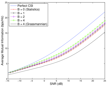
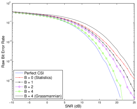
(a)	(b)

Figure 3: (a) Average mutual information with Gaussian inputs in a $4\times 4$ mismatched channel following a separable model. Two data-streams are used in signaling and a limited feedback codebook designed along the principle elucidated in Sec. IV is used. (b) Error probability performance with the same codebook under QPSK inputs.

VI Numerical Results

We now illustrate via numerical studies the performance gains possible with our codebook construction and the consequent bridging of the gap between statistical and optimal precoding. In the first study, we consider a $4\times 4$ channel under the separable model with ${\bf\Lambda}_{t}={\mathrm{diag}}\left([14.98\hskip 7.22743pt0.50\hskip 7.22743pt0.26\hskip 7.22743pt0.26]\right)$ and ${\bf\Lambda}_{r}={\mathrm{diag}}\left([15.5\hskip 7.22743pt0.25\hskip 7.22743pt0.15\hskip 7.22743pt0.10]\right)$. This choice ensures that the transmit$/$receive covariance matrices are both ill-conditioned and with $M=2$, note that the channel is not matched to the precoder. We first generate a root codeset of $N=4$ codewords with $\theta\approx 0.76$ and $\gamma\approx 0.75$ via VQ. Let $\{{\mathbf{u}}_{i}\}$ be the column vectors of ${\mathbf{U}}_{t}$. The codebook used for $B=1$ satisfies $N_{{\sf{stat}}}=1$ with the codeword corresponding to $[{\mathbf{u}}_{1}\hskip 3.61371pt{\mathbf{u}}_{2}]$ and $N_{{\sf{rvq}}}=1$ while with $B=2$, the codebook has an additional RVQ codeword and a local codeword around $[{\mathbf{u}}_{1}\hskip 3.61371pt{\mathbf{u}}_{2}]$. Similarly, with $B=4$, $N_{{\sf{stat}}}=3,N_{{\sf{loc}}}^{1}=N_{{\sf{loc}}}^{2}=3,N_{{\sf{loc}}}^{3}=2$ and $N_{{\sf{rvq}}}=5$. The statistical codewords correspond to $[{\mathbf{u}}_{1}\hskip 3.61371pt{\mathbf{u}}_{i}],\hskip 3.61371pti=2,\cdots,4$. Since we are mainly interested in illustrating the performance gains in the high-${\sf{SNR}}$ regime, uniform power allocation is used for ${\bf\Lambda}_{{\sf{stat}}}$.

Fig. 3(a) shows the average mutual information with a Gaussian input for statistical and limited feedback precoding. In addition to the mutual information, raw bit error rate (BER) is useful as well. Fig 3(b) shows the improvement in error probability in the same channel with QPSK inputs. In the error probability case, the index of the codeword that minimizes the distance to the instantaneous $\widetilde{\bf V}_{\bf H}$ is fed back. Note that while the performance gap between the optimal and the statistical schemes is significantly bridged in the error probability case, further improvement in mutual information is possible. Nevertheless, both the figures show that substantial gains are possible with a few bits of feedback. For example, with $B=4$ bits of feedback, a $3$ dB gain is possible at a rate of $10$ bps/Hz while a $6$ dB gain is possible at a BER of $10^{-3}$. Also, note that an i.i.d. codebook design incurs a dramatic loss in performance in correlated channels.

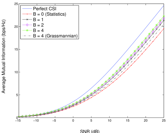
Figure 4: Average mutual information with Gaussian inputs in a $4\times 4$ mismatched channel with non-separable correlation and $M=3$.

In the second study, we consider a $4\times 4$ channel with non-separable correlation following the virtual representation framework. The variance matrix ${\bf\sigma}(i,j)\triangleq{\mathit{E}}\left[|{\mathbf{H}}_{{\sf{ind}}}(i,j)|^{2}\right]$ used in the study is

$${\bf\sigma}=\left[\begin{array}[]{cccc}1.24&1.42&7.49&0.23\\ 0.41&0.14&0.42&0.03\\ 0.72&1.39&0.07&0.02\\ 0.28&0.13&0.50&1.51\end{array}\right].$$ (33)

Note that the channel has a single dominant transmit (as well as receive) eigen-mode and is hence mismatched when $M=3$ data-streams are used in signaling. The parameters of the root codeset are $N=4,\hskip 3.61371pt\theta\approx 0.87$ and $\gamma\approx 0.84$. As before, let $\{{\mathbf{u}}_{i}\}$ be the column vectors of the DFT matrix ${\mathbf{U}}_{t}$. The codebook for $B=1$ has the two statistical codewords $[{\mathbf{u}}_{3}\hskip 3.61371pt{\mathbf{u}}_{2}\hskip 3.61371pt{\mathbf{u}}_{1}]$ and $[{\mathbf{u}}_{3}\hskip 3.61371pt{\mathbf{u}}_{2}\hskip 3.61371pt{\mathbf{u}}_{4}]$. For $B=2$, we use two additional RVQ codewords and for $B=4$, we use $N_{{\sf{stat}}}=3,N_{{\sf{loc}}}^{1}=N_{{\sf{loc}}}^{2}=3,N_{{\sf{loc}}}^{3}=2$ and $N_{{\sf{rvq}}}=5$. The third statistical codeword when $B=4$ is $[{\mathbf{u}}_{3}\hskip 3.61371pt{\mathbf{u}}_{1}\hskip 3.61371pt{\mathbf{u}}_{4}]$. Fig. 4 illustrates the bridging of the gap in mutual information between the optimal and the statistical schemes. It is important to note that both the channels studied here are so constructed to result in a substantial performance gap between perfect CSI and statistical signaling. In more realistic channels that are not so poorly matched, we expect an even better performance with our scheme. Thus our studies illustrate that substantial gains can be achieved even with few bits of feedback.

VII Concluding Remarks

In this work, we have studied linear precoding under a realistic system model. In particular, the focus is on the impact of spatial correlation when perfect CSI is available at the receiver, statistical information is available at both the ends, and quantized channel information is fed back from the receiver to the transmitter. While initial works on precoding assume perfect CSI at both the ends and hence do not impose any particular structure on the precoder matrices, under the model studied here, we see that structure can help in minimizing the reverse-link feedback as well as ease the implementation complexity.

We introduced the notion of matched and mismatched channels and illustrated that limited feedback precoding is useful only in the case of mismatched channels. The study of statistical precoding motivates the proposed limited feedback design where we quantize the space of semiunitary matrices with a non-uniform bias towards the statistically dominant eigen-modes. The design as well as its adaptability are rendered practical by the construction of mathematical maps (operations) that can rotate and scale submanifolds on the Grassmann manifold. More importantly, numerical studies show that the proposed designs yield significant improvement in performance when the channel is mismatched to the communication scheme.

This work is a first attempt at systematic precoder codebook design in single-user multi-antenna channels that exploits spatial correlation. Possible extensions are the study of more complex receiver architectures and performance analysis in the finite antenna, arbitrary ${\sf{SNR}}$ setting, along the lines of [29]. More work also needs to be done to understand the impact of spatial correlation on the performance of the proposed limited feedback scheme which could in turn drive the development of more efficient codebook constructions. Open issues that need further study include practical aspects like codebook designs for wideband channels, codebook designs based on Fourier$/$Hadamard matrices that are useful in achieving the bounded gain power amplifier architecture and hence, have found much interest in the standardization community, incorporating the cost of statistics acquisition in performance analysis [41], and more general scattering environment-independent channel decompositions [42] that mimic the physical model closely. The case of multi-user systems with feedback, which has attracted significant recent interest, is another area for study.

We close the paper by drawing attention to the philosophy that has guided this work. While deducing the structure of the optimal signaling scheme under general assumptions on spatial correlation and channel information seems extremely difficult, an alternative approach that partitions this problem into smaller sub-problems could be quite fruitful. The general idea of matching the rank of the precoding scheme to the number of dominant transmit eigenvalues with the resolution necessary to decide whether an eigenvalue is “dominant” or not being a function of the ${\sf{SNR}}$ reminds one of the classical source-channel matching paradigm [43]. Initial evidence seen in this paper also suggests that this partitioning provides a natural framework to understand the performance of limited feedback schemes.

-A Proof of Theorem 1

The efficacy of the rotation map is established if we can show the following:

1. ${\mathbf{G}}_{i}^{H}{\mathbf{G}}_{i}={\mathbf{I}}_{M}$ for all $i$,

2. ${\mathbf{G}}_{1}={\bf{V}}_{{\sf{target}}}$, and

3. $d_{{\mathrm{proj}},\hskip 1.4457pt2}({\mathbf{G}}_{1},{\mathbf{G}}_{i})=d_{{\mathrm{proj}},\hskip 1.4457pt2}({\bf{V}}_{1},{\bf{V}}_{i})$ for all $i$.

To prove 1), first note that ${\mathbf{U}}_{{\bf{V}}_{1}}$ and ${\mathbf{U}}_{{\bf{V}}_{{\sf{target}}}}$ are $N_{t}\times N_{t}$ unitary matrices. From the semiunitarity property of ${\bf{V}}_{i}$, ${\mathbf{G}}_{i}^{H}{\mathbf{G}}_{i}={\mathbf{I}}_{M}$ follows trivially. Using the unitary property of ${\mathbf{U}}_{{\bf{V}}_{1}}$ and the decomposition in the statement of the theorem, 2) also follows trivially. For 3), note that

$$d_{{\mathrm{proj}},\hskip 1.4457pt2}({\mathbf{G}}_{1},{\mathbf{G}}_{i}) = \lambda_{\max}\left({\mathbf{G}}_{1}{\mathbf{G}}_{1}^{H}-{\mathbf{G}}_{i}{\mathbf{G}}_{i}^{H}\right)$$ (34)

$$= \lambda_{\max}\left({\mathbf{U}}_{{\bf{V}}_{{\sf{target}}}}{\mathbf{U}}_{{\bf{V}}_{1}}^{H}\left({\bf{V}}_{1}{\bf{V}}_{1}^{H}-{\bf{V}}_{i}{\bf{V}}_{i}^{H}\right){\mathbf{U}}_{{\bf{V}}_{1}}{\mathbf{U}}_{{\bf{V}}_{{\sf{target}}}}^{H}\right)=d_{{\mathrm{proj}},\hskip 1.4457pt2}({\bf{V}}_{1},{\bf{V}}_{i}).$$

In the above chain of equalities, we have used the fact that $\lambda({\bf AB})=\lambda({\bf BA})$ and the unitary property of ${\mathbf{U}}_{{\bf{V}}_{1}}$ and ${\mathbf{U}}_{{\bf{V}}_{{\sf{target}}}}$. Thus the proof is complete.

-B Generalized Scaling Map

Theorem 2

Let ${\cal{R}}$ be a root codeset with packing density $\gamma$ and center ${\bf{V}}_{1}$. Let ${\mathbf{U}}_{{\mathbf{A}}}$ and ${\bf W}$ be arbitrary $M\times M$ unitary matrices and let ${\mathbf{U}}_{{\mathbf{B}}}$ be an arbitrary $(N_{t}-M)\times(N_{t}-M)$ unitary matrix. Given $\alpha\in(0,1)$ and $M\leq(N_{t}-M)$, for any ${\bf{V}}_{i}\in{\cal{R}}$, generate an $M\times M$ diagonal, positive-definite matrix ${\mathbf{\Lambda}}_{i}$ with: ${\mathbf{\Lambda}}_{\min}\triangleq\min_{j}{\mathbf{\Lambda}}_{i}(j)=1-\alpha^{2}\left(1-\lambda_{\min}({\bf{V}}_{1}^{H}{\bf{V}}_{i}{\bf{V}}_{i}^{H}{\bf{V}}_{1})\right)$ and ${\mathbf{\Lambda}}_{\max}\triangleq\max_{j}{\mathbf{\Lambda}}_{i}(j)\leq 1$. Then, define ${\mathbf{A}}_{i}$ as ${\mathbf{A}}_{i}={\mathbf{U}}_{{\mathbf{A}}}\hskip 1.4457pt{\mathbf{\Lambda}}_{i}^{1/2}\hskip 1.4457pt{\bf W}^{H}$. Define the $M\times M$ principal component of the $(N_{t}-M)\times M$ diagonal matrix ${{\mathbf{\Lambda}}}_{{\mathbf{B}}}$ as $\left({\mathbf{I}}_{M}-{\mathbf{\Lambda}}_{i}\right)^{1/2}$ and ${\mathbf{B}}_{i}$ as ${\mathbf{B}}_{i}={\mathbf{U}}_{{\mathbf{B}}}\hskip 1.4457pt{\mathbf{\Lambda}}_{{\mathbf{B}}}^{1/2}\hskip 1.4457pt{\bf W}^{H}$.

If $M>(N_{t}-M)$, for any ${\bf{V}}_{i}\in{\cal{R}}$, generate an $(N_{t}-M)\times(N_{t}-M)$ diagonal, positive-semidefinite matrix ${\bf\Gamma}_{i}$ with: ${\bf\Gamma}_{\max}\triangleq\max_{j}{\bf\Gamma}_{i}(j)=\alpha^{2}\left(1-\lambda_{\min}({\bf{V}}_{1}^{H}{\bf{V}}_{i}{\bf{V}}_{i}^{H}{\bf{V}}_{1})\right)$ and ${\bf\Gamma}_{\min}\triangleq\min_{j}{\bf\Gamma}_{i}(j)\geq 0$. Then, define ${\mathbf{B}}_{i}$ as ${\mathbf{U}}_{{\mathbf{B}}}\hskip 1.4457pt{\mathbf{\Lambda}}_{{\mathbf{B}}}^{1/2}\hskip 1.4457pt{\bf W}^{H}$ with the principal $(N_{t}-M)\times(N_{t}-M)$ component of ${\mathbf{\Lambda}}_{{\mathbf{B}}}$ being ${\bf\Gamma}_{i}$. Define ${\bf A}_{i}$ as ${\mathbf{A}}_{i}={\mathbf{U}}_{{\mathbf{A}}}\hskip 1.4457pt{\mathbf{\Lambda}}_{{\mathbf{A}}}\hskip 1.4457pt{\bf W}^{H}$ with the principal $(N_{t}-M)\times(N_{t}-M)$ component of ${\mathbf{\Lambda}}_{{\mathbf{A}}}$ being ${\mathbf{I}}_{N_{t}-M}-{\bf\Gamma}_{i}$ and the principal southeast component being ${\mathbf{I}}_{2M-N_{t}}$.

Then, the scaling map $s(\cdot)$ that leads to a packing density of $\gamma\alpha$ is given by

$$s({\bf{V}}_{i})={\bf{V}}_{1}\hskip 1.4457pt{\mathbf{A}}_{i}+{\bf{V}}_{1}^{{\sf{null}}}\hskip 1.4457pt{\mathbf{B}}_{i}$$ (35)

where ${\bf{V}}_{1}^{{\sf{null}}}$ is a representative of the null-space corresponding to ${\bf{V}}_{1}$.

Proof:

Let $r_{{\mathbf{U}}}$ denote the rotation effected by a unitary matrix ${\mathbf{U}}$. Since the scaling operation has to keep the center of a root codeset fixed, in the sequel, we use a fixed $N_{t}\times M$ matrix as the center instead of ${\bf{V}}_{1}$ which is dependent on the choice of ${\cal{R}}$. This is achieved by a composition of three operations:

$$s(\cdot)=r_{{\mathbf{U}}_{{\bf{V}}_{1}}}\odot s_{{\sf{vertex}}}\odot r_{{\mathbf{U}}_{{\bf{V}}_{1}}^{H}}(\cdot).$$ (36)

Here, $r_{{\mathbf{U}}_{{\bf{V}}_{1}}^{H}}(\cdot)$ rotates the root codeset to the canonical precoder $[{\mathbf{I}}_{M}\hskip 3.61371pt{\mathbf{O}}_{M\times(N_{t}-M)}]^{T}$ while $s_{{\sf{vertex}}}(\cdot)$ scales (shrinks) the canonical codeset by a factor $\alpha$ and $r_{{\mathbf{U}}_{{\bf{V}}_{1}}}$ rotates it back to the direction corresponding to ${\bf{V}}_{1}$. From the above definition of $s(\cdot)$, we have

$$s({\bf{V}}_{i})=\left[\begin{array}[]{cc}{\bf{V}}_{1}&{\bf{V}}_{1}^{{\sf{null}}}\end{array}\right]\hskip 3.61371pts_{{\sf{vertex}}}\left(\left[\begin{array}[]{c}{\bf{V}}_{1}^{H}\hskip 1.4457pt{\bf{V}}_{i}\\ {\bf{V}}_{1}^{{\sf{null}},H}\hskip 1.4457pt{\bf{V}}_{i}\end{array}\right]\right)=\left[\begin{array}[]{cc}{\bf{V}}_{1}&{\bf{V}}_{1}^{{\sf{null}}}\end{array}\right]\hskip 3.61371pt\left[\begin{array}[]{c}{\mathbf{A}}_{i}\\ {\mathbf{B}}_{i}\end{array}\right]={\bf V}_{1}{\bf A}_{i}+{\bf V}_{1}^{{\sf{null}}}{\bf B}_{i}$$ (43)

where we have used a partitioning $[{\mathbf{A}}_{i}^{T}{\hskip 3.61371pt}{\mathbf{B}}_{i}^{T}]^{T}$ for the $N_{t}\times M$ matrix $s_{{\sf{vertex}}}\left(\left[\begin{array}[]{c}{\bf{V}}_{1}^{H}\hskip 1.4457pt{\bf{V}}_{i}\\ {\bf{V}}_{1}^{{\sf{null}},H}\hskip 1.4457pt{\bf{V}}_{i}\end{array}\right]\right)$. In this partitioning, ${\mathbf{A}}_{i}$ is $M\times M$ and is of full rank while ${\mathbf{B}}_{i}$ is an $(N_{t}-M)\times M$ matrix.

Given that ${\bf{V}}_{1}^{H}{\bf{V}}_{1}={\mathbf{I}}_{M}$, ${\bf{V}}_{1}^{H}{\bf{V}}_{1}^{{\sf{null}}}={\mathbf{O}}_{M\times(N_{t}-M)}$ and ${\bf{V}}_{1}^{{\sf{null}},H}{\bf{V}}_{1}^{{\sf{null}}}={\mathbf{I}}_{N_{t}-M}$, the relationship ${\mathbf{A}}_{i}^{H}{\mathbf{A}}_{i}+{\mathbf{B}}_{i}^{H}{\mathbf{B}}_{i}={\mathbf{I}}_{M}$ ensures that $s({\bf V}_{i})$ is semiunitary. We show that ${\mathbf{A}}_{i}$ and ${\mathbf{B}}_{i}$ have to be as in the statement of the theorem so that the following properties of $s(\cdot)$ are met:

1. $d_{{\mathrm{proj}},\hskip 1.4457pt2}(s({\bf V}_{1}),s({\bf V}_{i}))=\alpha d_{{\mathrm{proj}},\hskip 1.4457pt2}({\bf V}_{1},{\bf V}_{i})$ for all $i$, and

2. $s({\bf V}_{1})={\bf V}_{1}$.

First, let us consider the distance scaling property. Assuming 2) (which we check subsequently) and following Prop. 1, we need

$$\lambda_{\max}({\mathbf{C}})=\lambda_{\max}\left({\bf{V}}_{1}{\bf{V}}_{1}^{H}-s({\bf{V}}_{i})s({\bf{V}}_{i})^{H}\right)=\alpha\sqrt{1-\lambda_{\min}({\bf{V}}_{1}^{H}{\bf{V}}_{i}{\bf{V}}_{i}^{H}{\bf{V}}_{1})}$$ (44)

where ${\mathbf{C}}\triangleq{\bf{V}}_{1}{\bf{V}}_{1}^{H}-{\bf{V}}_{1}{\mathbf{A}}_{i}{\mathbf{A}}_{i}^{H}{\bf{V}}_{1}^{H}-{\bf{V}}_{1}^{{\sf{null}}}{\mathbf{B}}_{i}{\mathbf{A}}_{i}^{H}{\bf{V}}_{1}^{H}-{\bf{V}}_{1}{\mathbf{A}}_{i}{\mathbf{B}}_{i}^{H}{\bf{V}}_{1}^{{\sf{null}},H}-{\bf{V}}_{1}^{{\sf{null}}}{\mathbf{B}}_{i}{\mathbf{B}}_{i}^{H}{\bf{V}}_{1}^{{\sf{null}},H}$. In the expansion for ${\mathbf{C}}$, we have used the relationship in (35). We can decompose ${\mathbf{C}}$ as ${\mathbf{C}}_{2}{\mathbf{C}}_{1}^{T}$ where

$$\begin{array}[]{cc}{{\mathbf{C}}_{1}^{T}=\left[\begin{array}[]{c}{\bf{V}}_{1}^{H}\\ {\mathbf{A}}_{i}^{H}{\bf{V}}_{1}^{H}\\ {\mathbf{B}}_{i}^{H}{\bf{V}}_{1}^{{\sf{null}},H}\\ {\mathbf{B}}_{i}^{H}{\bf{V}}_{1}^{{\sf{null}},H}\end{array}\right],}&{{\mathbf{C}}_{2}=\left[\begin{array}[]{cccc}{\bf{V}}_{1}({\mathbf{I}}_{M}-{\mathbf{A}}_{i}{\mathbf{A}}_{i}^{H})&-{\bf{V}}_{1}^{{\sf{null}}}{\mathbf{B}}_{i}&-{\bf{V}}_{1}{\mathbf{A}}_{i}&-{\bf{V}}_{1}^{{\sf{null}}}{\mathbf{B}}_{i}\end{array}\right]}.\end{array}$$ (51)

Note that the non-trivial eigenvalues of ${\bf A}{\bf B}$ are the same as those of ${\bf B}{\bf A}$. Hence, $\lambda_{\max}({\mathbf{C}})=\lambda_{\max}({\mathbf{C}}_{1}^{T}{\mathbf{C}}_{2})$. Using the facts ${\bf{V}}_{1}^{H}{\bf{V}}_{1}={\mathbf{I}}_{M}$, ${\bf{V}}_{1}^{H}{\bf{V}}_{1}^{{\sf{null}}}={\mathbf{O}}_{M\times(N_{t}-M)}$ and ${\bf{V}}_{1}^{{\sf{null}},H}{\bf{V}}_{1}^{{\sf{null}}}={\mathbf{I}}_{N_{t}-M}$, observe that the $4M\times 4M$ matrix ${\mathbf{C}}_{1}^{T}{\mathbf{C}}_{2}$ is given by

$${\mathbf{C}}_{1}^{T}{\mathbf{C}}_{2}=\left[\begin{array}[]{cccc}{\mathbf{I}}_{M}-{\mathbf{A}}_{i}{\mathbf{A}}_{i}^{H}&{\mathbf{O}}_{M}&-{\mathbf{A}}_{i}&{\mathbf{O}}_{M}\\ {\mathbf{A}}_{i}^{H}({\mathbf{I}}_{M}-{\mathbf{A}}_{i}{\mathbf{A}}_{i}^{H})&{\mathbf{O}}_{M}&-{\mathbf{A}}_{i}^{H}{\mathbf{A}}_{i}&{\mathbf{O}}_{M}\\ {\mathbf{O}}_{M}&-{\mathbf{B}}_{i}^{H}{\mathbf{B}}_{i}&{\mathbf{O}}_{M}&-{\mathbf{B}}_{i}^{H}{\mathbf{B}}_{i}\\ {\mathbf{O}}_{M}&-{\mathbf{B}}_{i}^{H}{\mathbf{B}}_{i}&{\mathbf{O}}_{M}&-{\mathbf{B}}_{i}^{H}{\mathbf{B}}_{i}\\ \end{array}\right].$$ (56)

We will now show that the largest eigenvalue of ${\mathbf{C}}_{1}^{T}{\mathbf{C}}_{2}$ can be computed in closed-form. For this, we need to solve for $\lambda$ by setting $\det({\mathbf{C}}_{1}^{T}{\mathbf{C}}_{2}-\lambda{\mathbf{I}}_{4M})=0$. Towards this computation, we need to use Lemma 2 following which, we have

$$\frac{\det({\mathbf{C}}_{1}^{T}{\mathbf{C}}_{2}-\lambda{\mathbf{I}}_{4M})}{\det(-{\mathbf{B}}_{i}^{H}{\mathbf{B}}_{i}-\lambda{\mathbf{I}}_{M})}=\det\left(\begin{array}[]{ccc}{\mathbf{I}}_{M}-{\mathbf{A}}_{i}{\mathbf{A}}_{i}^{H}-\lambda{\mathbf{I}}_{M}&{\mathbf{O}}_{M}&-{\mathbf{A}}_{i}\\ {\mathbf{A}}_{i}^{H}({\mathbf{I}}_{M}-{\mathbf{A}}_{i}{\mathbf{A}}_{i}^{H})&-\lambda{\mathbf{I}}_{M}&-{\mathbf{A}}_{i}^{H}{\mathbf{A}}_{i}\\ {\mathbf{O}}_{M}&-\lambda{\mathbf{B}}_{i}^{H}{\mathbf{B}}_{i}({\mathbf{B}}_{i}^{H}{\mathbf{B}}_{i}+\lambda{\mathbf{I}}_{M})^{-1}&-\lambda{\mathbf{I}}_{M}\\ \end{array}\right).$$ (60)

With $\kappa=\det(-{\mathbf{B}}_{i}^{H}{\mathbf{B}}_{i}-\lambda{\mathbf{I}}_{M})\det(-\lambda{\mathbf{I}}_{M})$, upon another application of Lemma 2 we have

$$\frac{\det({\mathbf{C}}_{1}^{T}{\mathbf{C}}_{2}-\lambda{\mathbf{I}}_{4M})}{\kappa}=\det\left(\begin{array}[]{cc}{\mathbf{I}}_{M}-{\mathbf{A}}_{i}{\mathbf{A}}_{i}^{H}-\lambda{\mathbf{I}}_{M}&{\mathbf{A}}_{i}{\mathbf{B}}_{i}^{H}{\mathbf{B}}_{i}({\mathbf{B}}_{i}^{H}{\mathbf{B}}_{i}+\lambda{\mathbf{I}}_{M})^{-1}\\ {\mathbf{A}}_{i}^{H}({\mathbf{I}}-{\mathbf{A}}_{i}{\mathbf{A}}_{i}^{H})&-\lambda{\mathbf{I}}_{M}+{\mathbf{A}}_{i}^{H}{\mathbf{A}}_{i}{\mathbf{B}}_{i}^{H}{\mathbf{B}}_{i}({\mathbf{B}}_{i}^{H}{\mathbf{B}}_{i}+\lambda{\mathbf{I}}_{M})^{-1}\end{array}\right)$$ (63)

which can be simplified to

$$\begin{split}&\hskip 7.22743pt\det({\mathbf{C}}_{1}^{T}{\mathbf{C}}_{2}-\lambda{\mathbf{I}}_{4M})\\ &{\hskip 21.68121pt}=\det(-{\mathbf{B}}_{i}^{H}{\mathbf{B}}_{i}-\lambda{\mathbf{I}}_{M})\det(-\lambda{\mathbf{I}}_{M})\det(-\lambda{\mathbf{I}}_{M}+{\mathbf{A}}_{i}^{H}{\mathbf{A}}_{i}{\mathbf{B}}_{i}^{H}{\mathbf{B}}_{i}({\mathbf{B}}_{i}^{H}{\mathbf{B}}_{i}+\lambda{\mathbf{I}}_{M})^{-1})\\ &{\hskip 21.68121pt}\times\det(-\lambda{\mathbf{I}}_{M}-\lambda{\mathbf{A}}_{i}^{-H}(-\lambda{\mathbf{I}}_{M}+{\mathbf{A}}_{i}^{H}{\mathbf{A}}_{i}{\mathbf{B}}_{i}^{H}{\mathbf{B}}_{i}({\mathbf{B}}_{i}^{H}{\mathbf{B}}_{i}+\lambda{\mathbf{I}}_{M})^{-1})^{-1}{\mathbf{A}}_{i}^{H}({\mathbf{I}}_{M}-{\mathbf{A}}_{i}{\mathbf{A}}_{i}^{H})).\end{split}$$

Note that $\det({\mathbf{C}}_{1}^{T}{\mathbf{C}}_{2}-\lambda{\mathbf{I}}_{4M})=0$ has $4M$ solutions for $\lambda$ with the solution from the first two terms being non-positive. Setting the fourth term to zero, and using the facts that $\det({\mathbf{I}}+{\mathbf{C}}{\mathbf{D}})=\det({\mathbf{I}}+{\mathbf{D}}{\mathbf{C}})$ and ${\mathbf{I}}_{M}={\mathbf{A}}_{i}^{H}{\mathbf{A}}_{i}+{\mathbf{B}}_{i}^{H}{\mathbf{B}}_{i}$, we see that $\lambda$ has to satisfy:

$$-1-\lambda_{i}((-\lambda{\mathbf{I}}_{M}+{\mathbf{A}}_{i}^{H}{\mathbf{A}}_{i}({\mathbf{I}}_{M}-{\mathbf{A}}_{i}^{H}{\mathbf{A}}_{i})({\mathbf{I}}_{M}+\lambda{\mathbf{I}}_{M}-{\mathbf{A}}_{i}^{H}{\mathbf{A}}_{i})^{-1})^{-1}({\mathbf{I}}_{M}-{\mathbf{A}}_{i}^{H}{\mathbf{A}}_{i}))=0.$$ (64)

After some straightforward simplifications, we can check that $\lambda$ is a solution to

$$\lambda_{i}(\lambda({\mathbf{I}}_{M}-{\mathbf{A}}_{i}^{H}{\mathbf{A}}_{i})^{-1}-{\mathbf{A}}_{i}^{H}{\mathbf{A}}_{i}({\mathbf{I}}_{M}+\lambda{\mathbf{I}}_{M}-{\mathbf{A}}_{i}^{H}{\mathbf{A}}_{i})^{-1})=1.$$ (65)

Assume a singular value decomposition for ${\mathbf{A}}_{i}$ and ${\mathbf{B}}_{i}$ of the form: ${\mathbf{A}}_{i}={\mathbf{U}}_{{\mathbf{A}}}{\mathbf{\Lambda}}_{{\mathbf{A}}}^{1/2}{\bf W}_{{\mathbf{A}}}^{H}$ and ${\mathbf{B}}_{i}={\mathbf{U}}_{{\mathbf{B}}}{\mathbf{\Lambda}}_{{\mathbf{B}}}^{1/2}{\bf W}_{{\mathbf{B}}}^{H}$, respectively where ${\mathbf{U}}_{{\mathbf{A}}},{\bf W}_{{\mathbf{A}}}$ and ${\bf W}_{{\mathbf{B}}}$ are $M\times M$ unitary matrices, and ${\mathbf{U}}_{{\mathbf{B}}}$ is an $(N_{t}-M)\times(N_{t}-M)$ unitary matrix. The full-rankness of ${\mathbf{A}}_{i}$ means that the $M\times M$ diagonal matrix ${\mathbf{\Lambda}}_{{\mathbf{A}}}$ is positive definite while the $(N_{t}-M)\times M$ matrix ${\mathbf{\Lambda}}_{{\mathbf{B}}}$ has non-negative entries only along the leading diagonal. Since ${\mathbf{A}}_{i}^{H}{\mathbf{A}}_{i}+{\mathbf{B}}_{i}^{H}{\mathbf{B}}_{i}={\mathbf{I}}_{M}$, we have ${\mathbf{I}}_{M}-{\mathbf{\Lambda}}_{{\mathbf{A}}}={\bf W}_{{\mathbf{A}}}^{H}{\bf W}_{{\mathbf{B}}}({\mathbf{\Lambda}}_{{\mathbf{B}}}^{T}{\mathbf{\Lambda}}_{{\mathbf{B}}})^{1/2}{\bf W}_{{\mathbf{B}}}^{H}{\bf W}_{{\mathbf{A}}}$. Comparing the two sides, we see that ${\bf W}_{{\mathbf{A}}}={\bf W}_{{\mathbf{B}}}$ (we set both to be ${\bf W}$) and ${\mathbf{I}}_{M}-{\mathbf{\Lambda}}_{{\mathbf{A}}}=({\mathbf{\Lambda}}_{{\mathbf{B}}}^{T}{\mathbf{\Lambda}}_{{\mathbf{B}}})^{1/2}$. Note that since there are no constraints on$/$relationship between ${\mathbf{U}}_{{\mathbf{A}}}$ and ${\mathbf{U}}_{{\mathbf{B}}}$, the leading diagonal entries of ${\mathbf{\Lambda}}_{{\mathbf{A}}}$ and ${\mathbf{\Lambda}}_{{\mathbf{B}}}$ can be in any order. This is because either unitary matrix can be appropriately adjusted by a permutation matrix.

Plugging in ${\mathbf{A}}_{i}^{H}{\mathbf{A}}_{i}={\bf W}{\mathbf{\Lambda}}_{{\mathbf{A}}}{\bf W}^{H}$ in (65), a routine computation yields $M$ solutions to $\lambda$ of the form: $\lambda^{2}=1-{\mathbf{\Lambda}}_{{\mathbf{A}}}(i)$. With the same form of ${\mathbf{A}}_{i}^{H}{\mathbf{A}}_{i}$, by setting the third term to zero, we obtain another $M$ solutions $\lambda=\sqrt{1-{\mathbf{\Lambda}}_{{\mathbf{A}}}(i)}\cdot\left(\frac{\sqrt{1+3{\mathbf{\Lambda}}_{{\mathbf{A}}}(i)}-\sqrt{1+{\mathbf{\Lambda}}_{{\mathbf{A}}}(i)}}{2}\right)$. Note that $\frac{\sqrt{1+3{\mathbf{\Lambda}}_{{\mathbf{A}}}(i)}-\sqrt{1+{\mathbf{\Lambda}}_{{\mathbf{A}}}(i)}}{2}<1$ and hence, $\lambda_{\max}({\mathbf{C}})$ is obtained by setting $i=M$ in the above solution which results in $\lambda_{\max}({\mathbf{C}})=\sqrt{1-\lambda_{\min}({\mathbf{A}}^{H}{\mathbf{A}})}$. Using this in (44), we get the expression for $\lambda_{\min}({\mathbf{A}}_{i}^{H}{\mathbf{A}}_{i})$. Furthermore, ${\mathbf{I}}_{M}={\mathbf{A}}_{i}^{H}{\mathbf{A}}_{i}+{\mathbf{B}}_{i}^{H}{\mathbf{B}}_{i}$ implies that

$$1=\lambda_{\max}({\mathbf{A}}_{i}^{H}{\mathbf{A}}_{i}+{\mathbf{B}}_{i}^{H}{\mathbf{B}}_{i})\geq\lambda_{\max}({\mathbf{A}}_{i}^{H}{\mathbf{A}}_{i})+\lambda_{\min}({\mathbf{B}}_{i}^{H}{\mathbf{B}}_{i})\geq\{\lambda_{\max}({\mathbf{A}}_{i}^{H}{\mathbf{A}}_{i}),\lambda_{\max}({\mathbf{B}}_{i}^{H}{\mathbf{B}}_{i})\}.$$ (66)

These are the constraints to be imposed on ${\mathbf{\Lambda}}_{{\mathbf{A}}}$ to ensure that the scaling map preserves semiunitarity and reduces the minimum distance by $\alpha$.

If $M\leq(N_{t}-M)$, without loss in generality assume that the diagonal entries of ${\mathbf{\Lambda}}_{{\mathbf{A}}}$ are in non-increasing order while those of ${\mathbf{\Lambda}}_{{\mathbf{B}}}$ may be not. Given a choice of ${\mathbf{\Lambda}}_{{\mathbf{A}}}$, the condition ${\mathbf{I}}_{M}-{\mathbf{\Lambda}}_{{\mathbf{A}}}=({\mathbf{\Lambda}}_{{\mathbf{B}}}^{T}{\mathbf{\Lambda}}_{{\mathbf{B}}})^{1/2}$ can be met by choosing the principal $M\times M$ component of ${\mathbf{\Lambda}}_{{\mathbf{B}}}$ to be $\left({\mathbf{I}}_{M}-{\mathbf{\Lambda}}_{{\mathbf{A}}}\right)^{1/2}$. If $M>(N_{t}-M)$, assume that the diagonal entries of ${\mathbf{\Lambda}}_{{\mathbf{B}}}$ are in non-increasing order while those of ${\mathbf{\Lambda}}_{{\mathbf{A}}}$ may be not. Then, the condition ${\mathbf{I}}_{M}-{\mathbf{\Lambda}}_{{\mathbf{A}}}=({\mathbf{\Lambda}}_{{\mathbf{B}}}^{T}{\mathbf{\Lambda}}_{{\mathbf{B}}})^{1/2}$ can be met if $2M-N_{t}$ entries of ${\mathbf{\Lambda}}_{{\mathbf{A}}}$ are $1$. The additional constraint on the smallest diagonal entry (see discussion above) ensures distance scaling.

To close the theorem, it is necessary to verify that $s({\bf{V}}_{1})={\bf{V}}_{1}$. This can be done by checking that ${\mathbf{\Lambda}}_{i}$ can be computed in closed-form. For this, note that ${\mathbf{\Lambda}}_{\min}=1$ and since ${\mathbf{\Lambda}}_{\max}\leq 1$, we have ${\mathbf{\Lambda}}_{i}={\mathbf{I}}_{M}$. From here, it can be checked that ${\mathbf{B}}_{i}={\mathbf{O}}_{(N_{t}-M)\times M}$ and from (35), we thus have $s({\bf{V}}_{1})={\bf{V}}_{1}\hskip 1.4457pt{\mathbf{U}}_{{\mathbf{A}}}\hskip 1.4457pt{\bf W}^{H}$. On the Grassmann manifold ${\cal{G}}(N_{t},M)$, multiplication by an $M\times M$ unitary matrix results in the same “point.” Thus $s({\bf{V}}_{1})={\bf{V}}_{1}$ and the proof is complete. ∎

Note that the choice of the scaling map is non-unique due to freedom in the choice of ${\mathbf{U}}_{{\mathbf{A}}}$, ${\mathbf{U}}_{{\mathbf{B}}}$ and ${\bf W}$ as well as the eigenvalues of ${\mathbf{\Lambda}}_{i}$ and ${\bf\Gamma}_{i}$. The case of ${\bf V}_{i}={\bf V}_{1}$ is special where ${\mathbf{\Lambda}}_{i}$ turns out to be ${\mathbf{I}}_{M}$. With almost any other choice of ${\bf{V}}_{i}$, these matrices are non-identity, in general. Besides these choices, non-uniqueness of the representative of ${\bf{V}}_{1}^{{\sf{null}}}$ also leads to non-uniqueness of the map.

References

• [1] V. Tarokh, N. Seshadri, and A. R. Calderbank, “Space-Time Codes for High Data Rate Wireless Communication: Performance Criterion and Code Construction,” IEEE Trans. Inform. Theory, vol. 44, no. 2, pp. 744–765, Mar. 1998.
• [2] Í. E. Telatar, “Capacity of Multi-Antenna Gaussian Channels,” Eur. Trans. Telecommun., vol. 10, pp. 2172–2178, 2000.
• [3] D. J. Love, R. W. Heath, Jr., W. Santipach, and M. L. Honig, “What is the Value of Limited Feedback for MIMO Channels?,” IEEE Commun. Magaz., vol. 42, no. 10, pp. 54–59, Oct. 2004.
• [4] V. Raghavan, J. H. Kotecha, and A. M. Sayeed, “Canonical Statistical Models for Correlated MIMO Fading Channels and Capacity Analysis,” Submitted, IEEE Trans. Inform. Theory, Nov. 2007, Available: [Online]. http://www.ifp.uiuc.edu/$\sim$vasanth.
• [5] W. Weichselberger, M. Herdin, H. Ozcelik, and E. Bonek, “A Stochastic MIMO Channel Model with Joint Correlation of Both Link Ends,” IEEE Trans. Wireless Commun., vol. 5, no. 1, pp. 90–100, Jan. 2006.
• [6] A. M. Tulino, A. Lozano, and S. Verdú, “Impact of Antenna Correlation on the Capacity of Multiantenna Channels,” IEEE Trans. Inform. Theory, vol. 51, no. 7, pp. 2491–2509, July 2005.
• [7] C. N. Chuah, J. M. Kahn, and D. N. C. Tse, “Capacity Scaling in MIMO Wireless Systems under Correlated Fading,” IEEE Trans. Inform. Theory, vol. 48, no. 3, pp. 637–650, Mar. 2002.
• [8] A. M. Sayeed, “Deconstructing Multi-Antenna Fading Channels,” IEEE Trans. Sig. Proc., vol. 50, no. 10, pp. 2563–2579, Oct. 2002.
• [9] A. M. Sayeed and V. V. Veeravalli, “Essential Degrees of Freedom in Space-Time Fading Channels,” Proc. 13th IEEE Intern. Symp. Personal Indoor and Mobile Radio Commun., vol. 4, pp. 1512–1516, Sept. 2002.
• [10] K. H. Lee and D. P. Petersen, “Optimal Linear Coding for Vector Channels,” IEEE Trans. Commun., vol. 24, no. 12, pp. 1283–1290, Dec. 1976.
• [11] J. Salz, “Digital Transmission over Cross-Coupled Linear Channels,” AT&T Tech. J., vol. 64, no. 6, pp. 1147–1159, July-Aug. 1985.
• [12] J. Yang and S. Roy, “On Joint Transmitter and Receiver Optimization for Multiple-Input-Multiple-Output (MIMO) Transmission Systems,” IEEE Trans. Commun., vol. 42, no. 12, pp. 3221–3231, Dec. 1994.
• [13] A. Scaglione, G. B. Giannakis, and S. Barbarossa, “Redundant Filterbank Precoders and Equalizers Part I: Unification and Optimal Designs,” IEEE Trans. Sig. Proc., vol. 47, no. 7, pp. 1988–2006, July 1999.
• [14] H. Sampath, P. Stoica, and A. Paulraj, “Generalized Linear Precoder and Decoder Design for MIMO Channels Using the Weighted MMSE Criterion,” IEEE Trans. Commun., vol. 49, no. 12, pp. 2198–2206, Dec. 2001.
• [15] H. Sampath and A. Paulraj, “Linear Precoding for Space-Time Coded Systems with Known Fading Correlations,” IEEE Commun. Letters, vol. 6, no. 6, pp. 239–241, June 2002.
• [16] J. Yang and S. Roy, “Joint Transmitter-Receiver Optimization for Multi-input Multi-output Systems with Decision Feedback,” IEEE Trans. Inform. Theory, vol. 40, no. 5, pp. 1334–1347, Sept. 1994.
• [17] A. Scaglione, P. Stoica, S. Barbarossa, G. B. Giannakis, and H. Sampath, “Optimal Designs for Space-Time Linear Precoders and Decoders,” IEEE Trans. Sig. Proc., vol. 50, no. 5, pp. 1051–1064, May 2002.
• [18] D. P. Palomar, J. M. Cioffi, and M. A. Lagunas, “Joint Tx-Rx Beamforming Design for Multicarrier MIMO Channels: A Unified Framework for Convex Optimization,” IEEE Trans. Sig. Proc., vol. 51, no. 9, pp. 2381–2401, Sept. 2003.
• [19] D. J. Love, R. W. Heath, Jr., and T. Strohmer, “Grassmannian Beamforming for Multiple-Input Multiple-Output Wireless Systems,” IEEE Trans. Inform. Theory, vol. 49, no. 10, pp. 2735–2747, Oct. 2003.
• [20] K. K. Mukkavilli, A. Sabharwal, E. Erkip, and B. Aazhang, “On Beamforming with Finite Rate Feedback in Multiple Antenna Systems,” IEEE Trans. Inform. Theory, vol. 49, no. 10, pp. 2562–2579, Oct. 2003.
• [21] W. Santipach, Y. Sun, and M. L. Honig, “Benefits of Limited Feedback for Wireless Channels,” Proc. Annual Allerton Conf. Commun. Control and Computing, Oct. 2003.
• [22] J. C. Roh and B. D. Rao, “Transmit Beamforming in Multiple-Antenna Systems with Finite Rate Feedback: A VQ-Based Approach,” IEEE Trans. Inform. Theory, vol. 52, no. 3, pp. 1101–1112, Mar. 2006.
• [23] D. J. Love and R. W. Heath, Jr., “Limited Feedback Diversity Techniques for Correlated Channels,” IEEE Trans. Veh. Tech., vol. 55, no. 2, pp. 718–722, Mar. 2006.
• [24] P. Xia and G. B. Giannakis, “Design and Analysis of Transmit Beamforming based on Limited-Rate Feedback,” IEEE Trans. Sig. Proc., vol. 54, no. 5, pp. 1853–1863, May 2006.
• [25] V. Raghavan, R. W. Heath, Jr., and A. M. Sayeed, “Systematic Codebook Designs for Quantized Beamforming in Correlated MIMO Channels,” IEEE Journ. Selected Areas in Commun., vol. 25, no. 7, pp. 1298–1310, Sept. 2007.
• [26] D. J. Love and R. W. Heath, Jr., “Limited Feedback Unitary Precoding for Spatial Multiplexing,” IEEE Trans. Inform. Theory, vol. 51, no. 8, pp. 2967–2976, Aug. 2005.
• [27] J. C. Roh and B. D. Rao, “Multiple Antenna Channels with Partial Channel State Information at the Transmitter,” IEEE Trans. Wireless Commun, vol. 3, no. 2, pp. 677–688, Mar. 2004.
• [28] D. J. Love and R. W. Heath, Jr., “Multimode Precoding for MIMO Wireless Systems,” IEEE Trans. Sig. Proc., vol. 53, no. 10, pp. 3674–3687, Oct. 2005.
• [29] V. Raghavan and A. M. Sayeed, “Impact of Spatial Correlation on Statistical Precoding in MIMO Channels with Linear Receivers,” Proc. Annual Allerton Conf. Commun. Control and Computing, Sept. 2006, Available: [Online]. http://www.ifp.uiuc.edu/$\sim$vasanth.
• [30] V. V. Veeravalli, Y. Liang, and A. M. Sayeed, “Correlated MIMO Rayleigh Fading Channels: Capacity, Optimal Signaling and Asymptotics,” IEEE Trans. Inform. Theory, vol. 51, no. 6, pp. 2058–2072, June 2005.
• [31] K. Yu, M. Bengtsson, B. Ottersten, D. McNamara, P. Karlsson, and M. Beach, “Second Order Statistics of NLOS indoor MIMO Channels based on 5.2 GHz Measurements,” Proc. IEEE Global Telecommun. Conf., vol. 1, pp. 25–29, Nov. 2001.
• [32] H. Ozcelik, M. Herdin, W. Weichselberger, J. Wallace, and E. Bonek, “Deficiencies of ’Kronecker’ MIMO Radio Channel Model,” Electronics Letters, vol. 39, no. 16, pp. 1209–1210, Aug. 2003.
• [33] J. Wallace, H. Ozcelik, M. Herdin, E. Bonek, and M. Jensen, “Power and Complex Envelope Correlation for Modeling Measured Indoor MIMO Channels: A Beamforming Evaluation,” Proc. 58th IEEE Fall Vehicular Technology Conference, 2003, vol. 1, pp. 363–367, Oct. 2003.
• [34] Y. Zhou, M. Herdin, A. M. Sayeed, and E. Bonek, “Experimental Study of MIMO Channel Statistics and Capacity via the Virtual Channel Representation,” Tech. Rep., University of Wisconsin-Madison, May 2006, Available: [Online]. http://dune.ece.wic.edu.
• [35] A. Barg and D. Yu. Nogin, “Bounds on Packings of Spheres in the Grassmann Manifolds,” IEEE Trans. Inform. Theory, vol. 48, no. 9, pp. 2450–2454, Sept. 2002.
• [36] A. Edelman, T. Arias, and S. Smith, “The Geometry of Algorithms with Orthogonality Constraints,” SIAM J. Matrix Anal. Appl., vol. 20, no. 2, pp. 303–353, Apr. 1999.
• [37] J. H. Conway, R. H. Hardin, and N. J. A. Sloane, “Packing Lines, Planes etc., Packings in Grassmannian Spaces,” Experimental Math., vol. 5, no. 2, pp. 139–159, 1996.
• [38] J. R. Silvester, “Determinants of Block Matrices,” The Mathematical Gazette, vol. 84, no. 501, pp. 460–467, Nov. 2000.
• [39] V. Raghavan, A. M. Sayeed, and N. Boston, “Near-Optimal Codebook Constructions for Limited Feedback Beamforming in Correlated MIMO Channels with Few Antennas,” Proc. IEEE Intern. Symp. Inform. Theory, pp. 2622–2626, July 2006.
• [40] R. Samanta and R. W. Heath, Jr., “Codebook Adaptation for Quantized MIMO Beamforming Systems,” Proc. IEEE Asilomar Conf. Signals, Systems and Computers, pp. 376–380, Nov. 2005.
• [41] V. Raghavan, A. S. Y. Poon, and V. V. Veeravalli, “Non-Robustness of Statistics Based Beamformer Design in Correlated MIMO Channels,” Proc. IEEE Intern. Conf. Acoustics, Speech and Sig. Proc., 2008.
• [42] V. Raghavan, A. S. Y. Poon, and V. V. Veeravalli, “MIMO Systems with Arbitrary Antenna Array Architectures: Channel Modeling, Capacity and Low-Complexity Signaling,” Proc. IEEE Asilomar Conf. Signals, Systems and Computers, Nov. 2007.
• [43] T. M. Cover and J. A. Thomas, Elements of Information Theory, Wiley Interscience, 1991.