Kolmogorov scaling from random force fields

Abstract

We show that the classical Kolmogorov and Richardson scaling laws in fully developed turbulence are consistent with a random Gaussian force field. Numerical simulations of a shell model approximation to the Navier-Stokes equations suggest that the fluctuations in the force (acceleration) field are scale independent throughout the inertial regime. We conjecture that Lagrangian statistics of the relative velocity in a turbulent flow is determined by the typical force field, whereas the multiscaling is associated to extreme events in the force field fluctuations.

In studies of fully developed turbulence, two discoveries are highly noticeable as fundamental and seminal. One regards L.R. Richardson’s study of the enhanced dispersion of particles advected by a turbulent flow Richardson26 . The other result is Kolmogorov’s fundamental derivation, essentially based on dimensional arguments, of the energy spectrum in fully developed turbulence Kolmogorov41 . Both theories employ the energy cascade, from the integral scale down to the dissipation scale, as the paradigmatic physical picture of the energy dissipation flow. Indeed, pair-particles passively advected by turbulence exhibit a superdiffusive behavior with their relative distance given by the Richardson’s scaling  Boffetta02 , Boffetta02bis . In contrast to the pair dispersion, the motion of a single particle is determined by the correlation time of the underlying velocity field, such that it is transported ballistically for times smaller than the correlation time and diffuses normally for larger time scales Falkovich01 . In the cascade scenario, the pair-particle superdiffusion is due to the large energy jumps between the eddies containing each particle. However, in the velocity space no superdiffusive behavior is needed to substantiate this jumpy motion.

In this Letter, we show that the velocity increments generated by a white-noise force field are sufficient to generate the superdiffusive behavior, as well as the Kolmogorov energy spectrum. To put it in very simple terms: integrating ’up’ from the random acceleration field to the velocity field and subsequently to the displacement is enough to reproduce the well-known scaling laws.

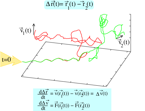
Figure 1: Two particles being advected in a random force field, generated by the GOY shell model.

To clarify the underlying physical picture, we consider a simple stochastic model of relative dispersion in a white noise acceleration field given by

$$\frac{d\Delta v}{dt} = \Delta F(t)$$ (1)

$$\langle\Delta F(t^{\prime})\Delta F(t")\rangle = 4\epsilon^{*}\;\delta(t^{\prime}-t"),$$ (2)

where $\Delta v(t)=v_{1}(t)-v_{2}(t)$ is the velocity difference between the two particles moving along the two trajectories $r_{1}(t)$ and $r_{2}(t)$, and $\Delta F(t)=F_{1}(t)-F_{2}(t)$ is the relative force. The prefactor $4$ instead of the usual factor $2$ appearing in the force correlation is due to the parametrization of the relative dispersion in terms of the diffusion constant $\epsilon^{*}$ for a single particle in the velocity space. The $\delta-$function may have, in principle, a finite width given by the time correlation of the relative random field along the two trajectories. This width will be determined both by the time it takes to pass a correlation length for a given force realization, and the time it takes to change the force in a certain point of the system.

In this set up, the relative velocity field, $\Delta v(t)=\int_{0}^{t}\Delta F(s)ds$, is a Wiener process with a Gaussian distribution, namely

$$\langle\Delta v(t_{1})\Delta v(t_{2})\rangle=4\epsilon^{*}\;min(t_{1},t_{2}),$$ (3)

while the relative separation is described by a non-Gaussian distribution with the second moment satisfying the Richardson’s scaling, that is

$$\langle\Delta r^{2}(t)\rangle=\frac{4\epsilon^{*}}{3}t^{3}.$$ (4)

By eliminating the time dependence of the relative velocity and distance, we obtain the exact Kolmogorov scaling,

$$\langle\Delta v^{2}(t)\rangle=48^{1/3}\epsilon^{*2/3}\langle\Delta r^{2}(t)\rangle^{1/3},$$ (5)

in the Lagrangian framework (for the higher moments see  moments ). Thus, Kolmogorov scaling is consistent with the assumption that the dispersion is driven by sufficiently random and uncorrelated acceleration fields.

In deriving Eq. (5) we assumed that the relative velocity is obtained by following the Lagrangian trajectories, which in a real turbulent flow may differ from the typical velocity increments separated by the distance $r$ (Eulerian measurement of the velocity differences) Mordant03 .

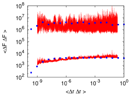
Figure 2: The squared relative acceleration $\Delta F\Delta F$ and its infinite moment versus $\Delta r^{2}$. The thin lines are for the Lagrangian trajectories where distances and accelerations are parameterized by the time of advection. The squares represent the corresponding Eulerian measures of the same quantities.

Eq. 4 implies that $2\epsilon^{*}$ is the diffusion constant for the relative velocity. For a Lagrangian stochastic flow generated by the white noise acceleration field, $\epsilon^{*}$ can be estimated as

$$\langle\Delta\vec{v}(t)\Delta\vec{F}(t)\rangle = \langle\int_{0}^{t}ds\Delta\vec{F}(s)\cdot\Delta\vec{F}(t)\rangle$$ (6)

$$= \int_{0}^{t}ds\langle\Delta\vec{F}(s)\cdot\Delta\vec{F}(t)\rangle$$

$$= 12\epsilon\int_{0}^{t}\delta(t-s)ds=12\epsilon^{*},$$

where the additional factor 3 compared to eq. 4 is related to the 3D system. From dimensional considerations, $\epsilon^{*}$ has the same units [$length^{2}/time^{3}$] as the standard energy dissipation rate $\epsilon$ characterizing the turbulence cascade.

To examine how the Lagrangian white-noise acceleration relates to the anomalous scaling laws in a more realistic turbulent field, we consider the kinematics of pair particles advected by the homogeneous turbulent flow obtained by a real-space transformation of the GOY shell model Jensen99 ; Bohr98 . This model proposed originally by Glenzer, Yamada and Ohkitani Gledzer73 ; Yamada87 provides a description of the turbulent motion embodied in the Navier-Stokes equations. The GOY model is formulated on a $N$-discrete set of wavenumbers, $k_{n}=2^{n}$, with the associated Fourier modes $u_{n}$ evolving according to

$$(\frac{d}{dt}+\nu k_{n}^{2})\ u_{n}\ = i\,k_{n}(a_{n}\,u^{*}_{n+1}u^{*}_{n+2}\,+\,\frac{b_{n}}{2}u^{*}_{n-1}u^{*}_{n+1}\,+\,$$ (7)

$$\frac{c_{n}}{4}\,u^{*}_{n-1}u^{*}_{n-2})\ +\ f\delta_{n,1},$$

for $n=1\cdots N$. The coefficients of the non-linear terms are constrained by two conservation laws, namely the total energy, $E=\sum_{n}|u_{n}|^{2}$, and the helicity (for 3d), $H=\sum_{n}(-1)^{n}k_{n}|u_{n}|$, or the enstrophy (for 2d), $Z=\sum_{n}k_{n}^{2}|u_{n}|^{2}$, in the inviscid limit, i.e. $f=\nu=0$ Biferale95 . Therefore, they may be expressed in terms of a free parameter only $\delta\in[0,2]$, $a_{n}=1,\ b_{n+1}=-\delta,\ c_{n+2}=-(1-\delta)$. As observed by Kadanoff Kadanoff95 , one obtains the canonical value $\epsilon=1/2$, when the 3d-helicity is conserved. The set (7) of $N$-coupled ordinary differential equations can be numerically integrated by standard techniques Pisarenko93 . We have used standard parameters in this paper $N=19,\nu=10^{-6},k_{0}=2\cdot 10^{-4},f=5\cdot 10^{-3}$.

The GOY model is defined in $k$-space but we study particle dispersion in direct space obtained by an inverse Fourier transform Jensen99 of the form

$${\vec{v}}({\vec{r}},t)=\sum_{n=1}^{N}{\vec{c}}_{n}[u_{n}(t)e^{i{\vec{k}}_{n}\cdot{\vec{r}}}+c.\,c.].$$ (8)

Here the wavevectors are ${\vec{k}}_{n}~{}=~{}k_{n}{\vec{e}}_{n}$ where ${\vec{e}}_{n}$ is a unit vector in a random direction, for each shell $n$ and ${\vec{c}}_{n}$ are unit vectors in random directions. We ensure that the velocity field is incompressible, $\nabla\cdot{\vec{v}}=0$, by constraining ${\vec{c}}_{n}\cdot{\vec{e}}_{n}=0,~{}\forall n$. In our numerical computations we consider the vectors ${\vec{c}}_{n}$ and ${\vec{e}}_{n}$ quenched in time but averaged over many different realizations of these.

As an example of the motion in this field, Fig. 1 shows the trajectories of two passively advected particles. As the relative distance diverges in time, the two particles experience different force fields, which in turn typically increase the difference in the relative velocities of the two particles. The figure shows the individual particles as they are advected, first together and later diverging away from each other when they are encased in different eddies.

Fig. 2 examines the noise in the effective force field $\langle\Delta F\Delta F\rangle$ for the relative motion of the two advected particles. In Fig 2a) we use viscosity $\nu=10^{-6}$, with a Kolmogorov scale $\Delta r\sim 1.0\cdot 10^{-4}$. The noise amplitude is plotted versus the average square distance between the particles $\langle\Delta r^{2}\rangle=\langle({\bf r}_{1}(t)-{\bf r}_{2}(t))^{2}\rangle$ , with the time as parametrization of the curves, as in eq. 5. The average is over independent trials of the two advected particles. One observes that both the typical noise and the maximum value at any distance is constant throughout the inertial range, i.e. above the Kolmogorov scale.

We conclude that the force field is equivalent to Gaussian white noise, and therefore the structure function of this turbulent field should be close to the one predicted by Eq. (5). This is confirmed in Fig. 3 where we show the deviations in velocity as a function of the square distance between the particles. One indeed sees that $\langle\Delta v^{2}(t)\rangle$ versus $\langle\Delta r^{2}(t)\rangle$ scales with an exponent close to $1/3$ in agreement with our expectations. For completeness, we also show the infinite moment of the velocity, and remark that this higher moment scales with an exponent close to $0.23$. This signals multidiffusion Sneppen94 where extreme velocity differences sometimes, but rarely, are reached after short separations. In the current context, we see these extreme deviations as a measure of very unlikely and intermittent events which only add little to the typical behavior of the flow. Indeed also the Eulerian statistics shows clear multiscaling as expected Jensen99 .

Figure 3: The squared relative velocity $(\Delta v)^{2}$ and its infinite moment versus $(\Delta r)^{2}$ (ie a representation of the structure function). The thin lines are for the Lagrangian trajectories where distances and velocities are parametriced by the time of advection. The filled squares represent are the corresponding Eulerian measures. The straight line represents standard Kolmogorov scaling $\langle\Delta v^{2}\rangle\propto\langle\Delta r^{2}\rangle^{1/3}$.

While our intuition has been based on the Lagrangian picture of advected particles, it is remarkable that the corresponding Eulerian quantities behaves similarly. This is demonstrated in simulations where we now fix the distance between two points, and then calculate respectively the difference in velocity and acceleration. The continuous curves in Figs. 2 and 3 show how $\langle\Delta F^{2}(r)\rangle$ and $\langle\Delta v^{2}(r)\rangle$ vary with the square relative distance between the investigated points. From Fig. 2 we see that the value of the plateau for the random force field is a direct consequence of its random expectation at any large distance. Therefore, there is nothing special about the selection of advected points in the Lagrangian case. In fact the onset of the plateau is slightly sharper in the Eulerian case, presumably reflecting averaging associated to the underlying time parameter in the Lagrangian advection. Similarly, there is no significant difference for the structure functions shown in Fig. 3.

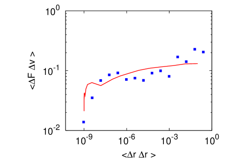
Figure 4: A measure of an effective diffusion constant in velocity: $\langle\Delta v\Delta F\rangle$ versus $\Delta r^{2}$. As in the previous figures the thin line describes Lagrangian trajectories parametriced by the time of advection. The filled squares correspond to the Eulerian case.

Using Eq. 6 we estimate $\langle\Delta v\Delta F\rangle\sim 0.1$ throughout the inertial range in the GOY model simulations, see Fig. 4. This value of the effective velocity diffusion constant is larger than the average energy dissipation at the Kolmogorov scale, estimated from the energy input ${\rm Re}\langle u_{1}^{*}\cdot f\rangle=0.001$ in the GOY model. This discrepancy in the effective diffusion terms we attribute to the huge contributions from the spikes in the acceleration which are absent in the simple white noise calculation of Eq. 6. These spikes also gives rise to multidiffusion, as discussed above.

We believe that the acceleration field as shown in Fig. 2 should be experimentally accessible either by particle tracking in a 3-D flow Luthi07 or from probe measurements in channel flows employing the Taylor hypothesis. In the first case the acceleration is easily estimated from the temporal variations in the velocity field of the 3-D advected particles.

Overall we have seen that the force field reaches an average value that is independent on the distance between the advected points in the turbulent fluid. Already at distances slightly above the Kolmogorov scale the two particles often receive random “kicks” which are as large at small scales as they are at the integral scale. Thus, huge accelerations are associated to the very small scales, presumably to the core of eddies at the verge of their destruction by dissipation. The acceleration between two particles are primarily dependent on how close each of them are to the center of an eddy. When examining the distribution of the accelerations at a fixed distance we observe a broad power law like behavior with a cutoff which is independent of the distance (as demonstrated by the constant max norm). The size of the cutoff is determined by the size of the forcing and the scale at which this forcing is acting (in our simulations, the scale is $\Delta r=1$).

In conclusion, the motion associated to the relatively slow turn over dynamics of the large eddies is not needed for obtaining Richardson or Kolmogorov statistics. These two seminal laws are primarily a consequence of the random force field that fluctuates with an amplitude set by the system size and with a correlation time set by the Kolmogorov scale.

We are grateful to Hiizu Nakanishi, Simone Pigolotti and Yves Pomeau for valuable discussions. We thank the Danish National Research Foundation for support through the Center for Models of Life.

References

- (1) L.F. Richardson, Proceedings of the Royal Society of London. Series A, 110, 756, pp. 709-737, 1926
- (2) A.N. Kolmogorov, C.R. Acad. Sci. USSR 30, 301; ibid 32, 16 (1941).
- (3) G. Boffetta and I.M. Sokolov, Physics of fluids, 14, 9, 2002
- (4) G. Boffetta and I.M. Sokolov, PRL, 88, 9, 2002
- (5) G. Falkovich and K. Gawedzki and M. Vergassola, Reviews of Modern Physics, 73, 2001
- (6) Using Wick’s theorem we obtain the -th moment of the velocity difference at time :
- (7) N. Mordant and J. Delour and E. Lveque and O. Michel and A. Arnodo and J.-F. Pinton, J. of Stat. Phys., 113, 5/6, 2003
- (8) M.H. Jensen, Phys.Rev.Lett. 83, 76 (1999).
- (9) T. Bohr and M.H. Jensen and G. Paladin and A. Vulpiani, Cambridge University Press, Cambridge, 1998
- (10) E. B. Gledzer, Sov. Phys. Dokl. 18, 216 (1973).
- (11) M. Yamada and K. Ohkitani, J. Phys. Soc. Japan 56, 4210(1987); Prog. Theor. Phys. 79,1265(1988).
- (12) L. Biferale, and R.M. Kerr, Phys. Rev. E 52, 6 (1995).
- (13) L. Kadanoff, D. Lohse, J. Wang, and R. Benzi, Phys. Fluids 7, 617 (1995).
- (14) D. Pisarenko, L. Biferale, D. Courvoisier, U. Frisch, and M. Vergassola, Phys. Fluids A5, 10 (1993).
- (15) K. Sneppen and M.H. Jensen, Phys.Rev.E 49, 919 (1994).
- (16) B. Lthi and J. Berg and S. Ott and J. Mann, Physics of Fluids 19, 2007