Non-linear response of molecular junctions:
The polaron model revisited

Abstract

A polaron model proposed as a possible mechanism for nonlinear conductance [Galperin M, Ratner M A, and Nitzan A 2005 Nano Lett. 5 125-30] is revisited with focus on the differences between the weak and strong molecule-lead coupling cases. Within the one-molecular level model we present an approximate expression for the electronic Green function corresponding to inelastic transport case, which in the appropriate limits reduces to expressions presented previously for the isolated molecule and for molecular junction coupled to a slow vibration (static limit). The relevance of considerations based on the isolated molecule limit to understanding properties of molecular junctions is discussed.

1 Introduction

Much of the interest in molecular conduction junctions stems from their functional properties as possible components in molecular electronic devices. In particular, non linear response behaviours such as bistability and negative differential resistance (NDR) have attracted much attention. Here we revisit a model for such phenomena that was previously advanced[1] and later criticized[2, 3, 4] in order to eludidate and clarify some of its mathematical characteristics.

The simplest molecular conduction junction comprises two metallic electrodes connected by a single molecule. The simplest theoretical model for such a junction is a molecule represented by one electronic level (the molecular affinity or ionization level) with one vibrational mode connecting free-electron metals. When the molecular electronic level is outside the range between the lead Fermi levels and its distance from these levels is large compared to the strength of the molecule-lead electronic coupling, the transport occurs by tunneling through the molecular energy barrier. This is the so-called Landauer-Imry limit. When the injection gap (distance between the Fermi level and the affinity or ionization levels) becomes small, the barrier decreases, and there is an opportunity for stabilizing excess charge on the molecule by polarization of its electronic and/or nuclear environment, leading to the formation of polaron-type trapped charge. We have previously described the consequences of this polarization on such phenomena as hysteresis, switching and negative differential resistance in molecular junctions.[1]

When the electronic coupling between the molecule and leads vanishes, one deals with polaron formation on an isolated molecule, for which an exact solution is available. We discuss here the two limiting cases: polaron formation on an isolated molecule, and the transport problem in the limit where nuclear dynamics is slow relative to all electronic timescales. Invoking the second case as one of the possible mechanisms of hysteresis, switching, and negative differential resistance in molecular junctions[1] was criticized by Alexandrov and Bratkovsky, in several papers.[2, 3, 4] These authors claim that the conclusions of Ref. [1] contradict a previously published “exact solution”[5, 6] that shows no multistability is possible for molecular models comprising nondegenerate and two-fold degenerate electronic levels. They suggest that multistability found in Ref. [1] is “an artifact of the mean-field approximation that neglects Fermi-Dirac statistics of electrons” ($\hat{n}_{0}^{2}=\hat{n}_{0}$), and “leads to a spurious self-interaction of a single polaron with itself and a resulting non-existent nonlinearity”.

As was pointed out previously,[7] the weakness of this criticism stems from using, in Ref. [5], the isolated quantum dot limit to discuss molecular junctions. In contrast, we have argued[7] that the approximtion of Ref. [1] is valid in the limit $\Gamma\gg\omega_{0}$, where $\Gamma$ is the inverse lifetime of excess carrier on the bridge and $\omega_{0}$ - the frequency of the relevant nuclear motion. Here we present this argument in a rigorous mathematical form. We describe a general approach to this problem, which is capable reproducing the result of Ref. [5] in the isolated molecule limit and our previous result, Ref. [1], in the static limit of a junction ($\omega_{0}/\Gamma\ll 1$), where $\omega_{0}$ is the oscillator frequency and $\Gamma$, the spectral density associated with the molecule-lead coupling, measures the strength of this coupling. This validates the polaronic approach of Ref. [1] in this limit.

2 General consideration

One way to bridge between the limits of zero and strong molecule-lead coupling is the nonequilibrium linked cluster expansion (NLCE) proposed in Ref. [8]. For our purposes a first order LCE[10] (clusters of second order in electron-phonon coupling $M$) is adequate. Indeed, this level of consideration provides exact results in both isolated molecule and static limits, while providing an approximate expression for the general case. The main idea of the NLCE is the same as in the usual LCE – one expands a Green function (GF) perturbatively in terms of the interaction part of the Hamiltonian (in our case - the electron-phonon interaction) up to some finite order, and equates the expansion in clusters to an expression in terms of cumulants.[9] This provides approximate resummation of the whole series.[10] The NLCE considers this expansion on the Keldysh contour[8]

$$G(\tau,\tau^{\prime})=\sum_{n=0}^{\infty}\xi^{n}W_{n}(\tau,\tau^{\prime})=G_{0}(\tau,\tau^{\prime})\exp\left[\sum_{n=1}^{\infty}\xi^{n}F_{n}(\tau,\tau^{\prime})\right]$$ (1)

whence, up to first order ($n=1$)

$$W_{0}(\tau,\tau^{\prime})=G_{0}(\tau,\tau^{\prime})\qquad W_{1}(\tau,\tau^{\prime})=G_{0}(\tau,\tau^{\prime})F_{1}(\tau,\tau^{\prime})$$ (2)

Projections of (1) on the real time axis are obtained using Langreth rules[11, 12], in particular

$$G^{>,<}(t,t^{\prime}) = G_{0}^{>,<}(t,t^{\prime})\exp\left[\sum_{n=1}^{\infty}\xi^{n}F_{n}^{>,<}(t,t^{\prime})\right]$$ (3)

$$W_{0}^{>,<}(t,t^{\prime}) = G_{0}^{>,<}(t,t^{\prime})$$ (4)

$$W_{1}^{>,<}(t,t^{\prime}) = G_{0}^{>,<}(t,t^{\prime})\,F_{1}^{>,<}(t,t^{\prime})$$ (5)

In steady state (which we consider below) projections depend on time difference $t-t^{\prime}$ only.

3 Model

As in Ref. [1] we consider a single (nondegenerate) electron level $\varepsilon_{0}$ coupled to one vibration $\omega_{0}$ and to two leads $L$ and $R$ represented by reservoirs of free electrons, each in its own equilibrium. The vibration is represented by a free oscillator at thermal equilibrium. The Hamiltonian of the system is (here and below $e=1$, $m=1$, and $\hbar=1$)

$$\hat{H} = \varepsilon_{0}\hat{d}^{\dagger}\hat{d}+\sum_{k\in\{L,R\}}\left(\varepsilon_{k}\hat{c}_{k}^{\dagger}\hat{c}_{k}+V_{k}\hat{d}^{\dagger}\hat{c}_{k}+V_{k}^{*}\hat{c}_{k}^{\dagger}\hat{d}\right)$$ (6)

$$+ \omega_{0}\hat{a}^{\dagger}\hat{a}+M(\hat{a}+\hat{a}^{\dagger})\hat{d}^{\dagger}\hat{d}$$

where $\hat{d}$ ($\hat{d}^{\dagger}$) and $\hat{c}_{k}$ ($\hat{c}_{k}^{\dagger}$) are annihilation (creation) operators for electrons on the molecule and in the contacts respectively, while $\hat{a}$ ($\hat{a}^{\dagger}$) are annihilation (creation) operators of a vibrational quantum. The first and second terms in (6) represent electrons on the bridge and in the contacts, respectively and the third and fourth terms describe molecule-leads coupling. The fifth term describes the free vibration, while the last is the linear electron-phonon coupling. For future reference we also define the operator of molecular level population

$$\hat{n}_{0}=\hat{d}^{\dagger}\hat{d}$$ (7)

and its quantum and statistical average

$$n_{0}=<\hat{n}_{0}>=-i\int_{-\infty}^{+\infty}\frac{dE}{2\pi}G^{<}(E)\equiv-iG^{<}(t=0)$$ (8)

where $G^{<}$ is the electron lesser GF.[9, 12]

4 Mathematical evaluation of transport properties

The non-equilibrium Green function technique provides a convenient framework for evaluating the desired transport properties. To obtain the steady-state current under given bias conditions

$$I_{K}=\frac{e}{\hbar}\int_{-\infty}^{+\infty}dt\,\mbox{Tr}\left[\Sigma_{K}^{<}(-t)\,G^{>}(t)-\Sigma_{K}^{>}(-t)\,G^{<}(t)\right]$$ (9)

($K=L,R$) one needs to evaluate the molecular electronic Green function in the presence of the moleule-lead and electron-phonon couplings. In what follows we derive this expression within the low-order NLCE described in Section 2.

The free phonon GFs (retarded, advanced, lesser and greater) are

$$D_{0}^{r}(t) = -i\theta(t)\left[e^{-i\omega_{0}t}-e^{i\omega_{0}t}\right]$$ (10)

$$D_{0}^{a}(t) = i\theta(-t)\left[e^{-i\omega_{0}t}-e^{i\omega_{0}t}\right]$$ (11)

$$D_{0}^{<}(t) = -i\left[(1+N_{0})e^{i\omega_{0}t}+N_{0}e^{-i\omega_{0}t}\right]$$ (12)

$$D_{0}^{>}(t) = -i\left[(1+N_{0})e^{-i\omega_{0}t}+N_{0}e^{i\omega_{0}t}\right]$$ (13)

where $N_{0}=[e^{\omega_{0}/T}-1]^{-1}$ is the thermal equilibrium vibration population.

In the absence of electron-phonon coupling, $M=0$, electron GFs in the wide band approximation (where the spectral densities $\Gamma_{K}=2\pi\sum_{k\in K}|V_{k}|^{2}\delta(E-\varepsilon_{k})$ are energy independent) are

$$G_{0}^{r}(t) = -i\theta(t)\,\exp\left[-i\varepsilon_{0}t-\frac{\Gamma}{2}t\right]$$ (14)

$$G_{0}^{a}(t) = i\theta(-t)\exp\left[-i\varepsilon_{0}t+\frac{\Gamma}{2}t\right]$$ (15)

$$G_{0}^{<}(t) = i\int_{-\infty}^{+\infty}\frac{dE}{2\pi}\,e^{-iEt}\frac{\Gamma_{L}f_{L}(E)+\Gamma_{R}f_{R}(E)}{(E-\varepsilon_{0})^{2}+(\Gamma/2)^{2}}$$ (16)

$$\approx in_{0}\exp\left[-i\varepsilon_{0}t-\frac{\Gamma}{2}|t|\right]$$

$$G_{0}^{>}(t) = -i\int_{-\infty}^{+\infty}\frac{dE}{2\pi}\,e^{-iEt}\frac{\Gamma_{L}[1-f_{L}(E)]+\Gamma_{R}[1-f_{R}(E)]}{(E-\varepsilon_{0})^{2}+(\Gamma/2)^{2}}$$ (17)

$$\approx -i[1-n_{0}]\exp\left[-i\varepsilon_{0}t-\frac{\Gamma}{2}|t|\right]$$

$\Gamma_{K}$ ($K=L,R$) are the electron escape rates from the molecule due to coupling to left and right leads, $\Gamma=\Gamma_{L}+\Gamma_{R}$ and $f_{K}(E)=[e^{(E-\mu_{k})/T}+1]^{-1}$ is the Fermi-Dirac distribution in the contact $K$ ($\mu_{K}$ is chemical potential). In approximations made in (16) and (17) we have used $n_{0}\approx\left(\Gamma_{L}f_{L}(\varepsilon_{0})+\Gamma_{R}f_{R}(\varepsilon_{0})\right)/\Gamma$. Note that these approximations are used for convenience only and do not influence the generality of the considerations below. They become exact either in the case of molecule weakly coupled to contacts or when molecular level is far (compared to $\Gamma$) from the contacts’ chemical potentials.

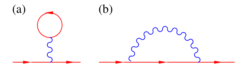
Figure 1: Lowest ($M^{2}$) order contributions to electron GF ($W_{1}$): (a) Hartree and (b) Fock (Born) terms. The wavy line represents free phonon GF. The straight line represents electron GF.

The lowest order in the electron-phonon coupling ($M^{2}$) contribution to the electronic GF is given by

$$W_{1}(\tau,\tau^{\prime}) = \int_{c}d\tau_{1}\int_{c}d\tau_{2}\,G_{0}(\tau,\tau_{1})\,\Sigma_{ph}(\tau_{1},\tau_{2})\,G_{0}(\tau_{2},\tau^{\prime})$$ (18)

$$\Sigma_{ph}(\tau_{1},\tau_{2}) = \delta(\tau_{1},\tau_{2})M^{2}n_{0}\int_{c}d\tau_{3}D_{0}(\tau_{1},\tau_{3})+iM^{2}D_{0}(\tau_{1},\tau_{2})\,G_{0}(\tau_{1},\tau_{2})$$ (19)

where self-energy (SE) $\Sigma_{ph}$ is a sum of two contributions: the first and second terms in Eq.(19) are respectively the Hartree and Born terms shown in Fig. 1. The importance of including the Hartree term when considering systems without translational periodicity (e.g. molecular junctions) was emphasized in a number of papers.[13, 14, 8]

The lesser and greater projections of (18) onto the real time axis (here and below we assume steady-state situation) are obtained from the Langreth rules[11, 12] as

$$W_{1}^{>,<}(t)=\int_{-\infty}^{+\infty}dt_{1}\int_{-\infty}^{+\infty}dt_{2}\,\left[G_{0}^{r}(t-t_{1})\,\Sigma_{ph}^{>,<}(t_{1}-t_{2})\,G_{0}^{a}(t_{2})\right.$$ (20)

$$+\left.G_{0}^{>,<}(t-t_{1})\,\Sigma_{ph}^{a}(t_{1}-t_{2})\,G_{0}^{a}(t_{2})+G_{0}^{r}(t-t_{1})\,\Sigma_{ph}^{r}(t_{1}-t_{2})\,G_{0}^{>,<}(t_{2})\right]$$

Projecting (19) and using Eqs. (10)-(17) one gets

$$\Sigma_{ph}^{r}(t) = -iM^{2}\theta(t)\left[(N_{0}+1-n_{0})e^{-i\omega_{0}t}+(N_{0}+n_{0})e^{i\omega_{0}t}\right]e^{-i\varepsilon_{0}t-\Gamma t/2}$$ (21)

$$- \delta(t)\frac{2M^{2}n_{0}}{\omega_{0}}$$

$$\Sigma_{ph}^{a}(t) = iM^{2}\theta(-t)\left[(N_{0}+1-n_{0})e^{-i\omega_{0}t}+(N_{0}+n_{0})e^{i\omega_{0}t}\right]e^{-i\varepsilon_{0}t+\Gamma t/2}$$ (22)

$$- \delta(t)\frac{2M^{2}n_{0}}{\omega_{0}}$$

$$\Sigma_{ph}^{<}(t) = iM^{2}n_{0}e^{-i\varepsilon_{0}t-\Gamma|t|/2}\left[(1+N_{0})e^{i\omega_{0}t}+N_{0}e^{-i\omega_{0}t}\right]$$ (23)

$$\Sigma_{ph}^{>}(t) = -iM^{2}[1-n_{0}]e^{-i\varepsilon_{0}t-\Gamma|t|/2}\left[(1+N_{0})e^{-i\omega_{0}t}+N_{0}e^{i\omega_{0}t}\right]$$ (24)

It should be emphasized that the $n_{0}$ term that enters the Hartree contribution in Eqs. (19), (21) and (22) is an exact result; unrelated to the convenient approximation made in Eqs. (16) and (17) above (that leads to the explicit appearance of the $n_{0}$ terms in Eqs. (23) and (24)). It is this term which will provide the population dependent shift of the electronic level in the static limit (see below).

Our aim is to get an expression for the retarded electron GF

$$G^{r}(t)=\theta(t)\left[G^{>}(t)-G^{<}(t)\right]$$ (25)

using (3)-(5). In order to do so we have to calculate $W_{1}^{>,<}$ which is given by Eq.(20). It is convenient to consider separately the first term and the sum of the second and third terms on the right-hand-side in (20)

$$W_{1}^{>,<}(t) = {\cal W}_{1}^{>,<}(t)+{\cal W}_{2}^{>,<}(t)$$ (26)

$${\cal W}_{1}^{>,<}(t) = \int_{-\infty}^{+\infty}dt_{1}\int_{-\infty}^{+\infty}dt_{2}\,G_{0}^{r}(t-t_{1})\,\Sigma_{ph}^{>,<}(t_{1}-t_{2})\,G_{0}^{a}(t_{2})$$ (27)

$${\cal W}_{2}^{>,<}(t) = \int_{-\infty}^{+\infty}dt_{1}\int_{-\infty}^{+\infty}dt_{2}\,\left[G_{0}^{>,<}(t-t_{1})\,\Sigma_{ph}^{a}(t_{1}-t_{2})\,G_{0}^{a}(t_{2})\right.$$ (28)

$$\left.\qquad\qquad\qquad\quad+G_{0}^{r}(t-t_{1})\,\Sigma_{ph}^{r}(t_{1}-t_{2})\,G_{0}^{>,<}(t_{2})\right]$$

utilizing (14)-(17) and (21)-(24) then leads to

$${\cal W}_{1}^{<}(t)=in_{0}e^{-i\varepsilon_{0}t-\Gamma|t|/2}\frac{M^{2}}{\omega_{0}}$$ (29)

$$\times\left\{\theta(t)\left[(1+N_{0})\left(\frac{e^{i\omega_{0}t}}{\omega_{0}+i\Gamma}+\frac{1}{\omega_{0}-i\Gamma}\right)+N_{0}\left(\frac{e^{-i\omega_{0}t}}{\omega_{0}-i\Gamma}+\frac{1}{\omega_{0}+i\Gamma}\right)\right]\right\}$$

$$+\left.\theta(-t)\left[(1+N_{0})\left(\frac{e^{i\omega_{0}t}}{\omega_{0}-i\Gamma}+\frac{1}{\omega_{0}+i\Gamma}\right)+N_{0}\left(\frac{e^{-i\omega_{0}t}}{\omega_{0}+i\Gamma}+\frac{1}{\omega_{0}-i\Gamma}\right)\right]\right\}$$

$${\cal W}_{2}^{<}(t)=-in_{0}e^{-i\varepsilon_{0}t-\Gamma|t|/2}\frac{M^{2}}{\omega_{0}}$$

$$\times\left\{\theta(t)\left[(N_{0}+1-n_{0})\left(\frac{1}{\omega_{0}+i\Gamma}+\frac{1}{\omega_{0}}-it+e^{-i\omega_{0}t}\left[\frac{1}{\omega_{0}-i\Gamma}-\frac{1}{\omega_{0}}\right]\right)\right.\right.$$

$$\qquad\qquad\left.+(N_{0}+n_{0})\left(\frac{1}{\omega_{0}-i\Gamma}+\frac{1}{\omega_{0}}+it+e^{i\omega_{0}t}\left[\frac{1}{\omega_{0}+i\Gamma}-\frac{1}{\omega_{0}}\right]\right)\right]$$ (30)

$$+\theta(-t)\left[(N_{0}+1-n_{0})\left(\frac{1}{\omega_{0}-i\Gamma}+\frac{1}{\omega_{0}}-it+e^{-i\omega_{0}t}\left[\frac{1}{\omega_{0}+i\Gamma}-\frac{1}{\omega_{0}}\right]\right)\right.$$

$$\qquad\qquad\left.+(N_{0}+n_{0})\left(\frac{1}{\omega_{0}+i\Gamma}+\frac{1}{\omega_{0}}+it+e^{i\omega_{0}t}\left[\frac{1}{\omega_{0}-i\Gamma}-\frac{1}{\omega_{0}}\right]\right)\right]$$

$$\quad-\left.2in_{0}t\right\}$$

The last term in curly brackets on the right-hand-side in (4) comes from the Hartree term. The expression for ${\cal W}_{1}^{>}(t)$ is obtained from (29) by interchanging $N_{0}$ and $N_{0}+1$ and replacing $n_{0}$ by $n_{0}-1$. ${\cal W}_{2}^{>}(t)$ is obtained from (4) by replacing $n_{0}$ by $n_{0}-1$ only in the prefactor that multiplies the curly brackets on the right-hand-side. These general approximate (first order LCE) expressions for ${\cal W}^{>,<}_{1,2}$ are the central result of this consideration.

5 Two physical limits

In [1] we have discussed a mean field approach to describe non-linear response of molecular junctions characterised by strong molecule-lead coupling as well as slow vibrations strongly coupled to the electronic subsystem. As noted in the introduction this approach was criticised in Refs. [2, 3, 4] as incompatible with observations made in the isolated molecule. To elucidate the issue we consider next these two specific limits: the isolated molecule ($\Gamma\to 0$) and static limit ($\omega_{0}/\Gamma\to 0$).

The isolated molecule

In the limit $\Gamma\to 0$ Eqs. (29) and (4) yield

$${\cal W}_{1}^{<}(t) = in_{0}e^{-i\varepsilon_{0}t}\frac{M^{2}}{\omega_{0}^{2}}$$ (31)

$$\times \left[(2N_{0}+1)+(1+N_{0})e^{i\omega_{0}t}+N_{0}e^{-i\omega_{0}t}\right]$$

$${\cal W}_{2}^{<}(t) = in_{0}e^{-i\varepsilon_{0}t}\left[-2\frac{M^{2}}{\omega_{0}^{2}}(2N_{0}+1)+i\frac{M^{2}}{\omega_{0}}t\right]$$ (32)

and the corresponding expressions for ${\cal W}_{1,2}^{>}(t)$

$${\cal W}_{1}^{>}(t) = -i[1-n_{0}]e^{-i\varepsilon_{0}t}\frac{M^{2}}{\omega_{0}^{2}}$$ (33)

$$\times \left[(2N_{0}+1)+(1+N_{0})e^{-i\omega_{0}t}+N_{0}e^{i\omega_{0}t}\right]$$

$${\cal W}_{2}^{>}(t) = -i[1-n_{0}]e^{-i\varepsilon_{0}t}\left[-2\frac{M^{2}}{\omega_{0}^{2}}(2N_{0}+1)+i\frac{M^{2}}{\omega_{0}}t\right]$$ (34)

Substituting (31)-(34) into (26) and using Eqs. (3) and (5), one gets from (25)

$$G^{r}(t) = -i\theta(t)e^{-i(\varepsilon_{0}-\Delta)t}e^{-\lambda^{2}(2N_{0}+1)}$$

$$\times \left\{(1-n_{0})\exp\left(\lambda^{2}\left[N_{0}e^{i\omega_{0}t}+(1+N_{0})e^{-i\omega_{0}t}\right]\right)\right.$$

$$+ \left.\qquad n_{0}\quad\,\,\exp\left(\lambda^{2}\left[N_{0}e^{-i\omega_{0}t}+(1+N_{0})e^{i\omega_{0}t}\right]\right)\right\}$$

where

$$\Delta\equiv\frac{M^{2}}{\omega_{0}}\qquad\lambda\equiv\frac{M}{\omega_{0}}$$ (36)

Eq.(5) is the standard expression for the retarded Green function in the isolated molecule case, obtained following a small polaron (Lang-Firsov or canonical) transformation.[9] In particular, it is identical to Eq.(30) of Ref. [5] for the case of a nondegenerate level (i.e. $d=1$ there). Note that approximations (16) and (17) become exact in this limit and, furthermore, the first order LCE provides the exact result in this limit. As was pointed out by Alexandrov and Bratkovsky[2, 3, 4] the electronic level shift, $\Delta$, is independent of level population for the isolated molecule, and no multistability is possible in this case.

The static limit

The $\omega_{0}/\Gamma\to 0$ limit reflects either a slow vibration or a strong molecule-lead coupling. For molecules chemisorbed on metal and semiconductor surfaces $\Gamma$ is often of order $0.1-1$ eV, so this limit is expected to be relevant for the relatively slow molecular motions associated with molecular configuration changes. To describe the behaviour of our model system in this case we expand the exponentials and the fractions in Eqs. (29) and (4) in powers of $\omega_{0}/\Gamma$, disregarding terms of order higher than $1$ and keeping in mind that due to the $e^{-\Gamma|t|/2}$ prefactor $\omega_{0}/\Gamma\sim\omega_{0}t$ holds. This implies

$$e^{\pm i\omega_{0}t}\approx 1\pm i\omega_{0}t\qquad\frac{1}{\omega_{0}\pm i\Gamma}\approx\frac{1}{\pm i\Gamma}\left(1\mp\frac{\omega_{0}}{i\Gamma}\right)$$ (37)

which leads to

$${\cal W}_{1}^{<}(t) = 0$$ (38)

$${\cal W}_{2}^{<}(t) = in_{0}e^{-i\varepsilon_{0}t-\Gamma|t|/2}\,i\frac{2M^{2}n_{0}}{\omega_{0}}t$$ (39)

and corresponding expressions for ${\cal W}_{1,2}^{>}(t)$

$${\cal W}_{1}^{>}(t) = 0$$ (40)

$${\cal W}_{2}^{>}(t) = -i[1-n_{0}]e^{-i\varepsilon_{0}t-\Gamma|t|/2}\,i\frac{2M^{2}n_{0}}{\omega_{0}}t$$ (41)

Substituting (38)-(41) into (26) and using the result in (3) and (5), one gets from (25)

$$G^{r}(t)=-i\theta(t)e^{-i(\varepsilon_{0}-2n_{0}\Delta)t-\Gamma t/2}$$ (42)

Again we note that the factor $n_{0}$ that enters this expression does not result from approximations (16) and (17). Rather, it arises from the exact expression for the Hartree term, the first term on the right-hand-side in Eq.(19). Note also, that the approximation used in Eqs. (16) and (17) could in principle be relaxed. This would make the mathematical evaluation more difficult (unless the molecular level is far, compared to $\Gamma$, from the leads’ chemical potentials, when this approximation becomes exact) but would not influence the estimates of ${\cal W}_{1,2}^{>,<}$ in terms of $\omega_{0}/\Gamma$.

Note that technically the static limit corresponds to disregarding all diagrams (in all orders of electron-phonon interaction) except the Hartree term (see Fig. 1a) and terms of similar character (only diagrams with boson lines terminated in a closed loop), since these are the only diagrams transmitting zero frequency. In the static limit this is not a mean-field approximation but an exact result. Detailed discussion on the issue can be found in Ref. [14].

To conclude, in the static limit (which is the limit considered in Ref. [1]) the electronic level shift, $2n_{0}\Delta$, does depend on level population in the way presented in our polaron model.[1] In what follows we briefly reiterate the implications of this observation on the conduction properties of molecular junctions with strong coupling between the electronic and nuclear subsystem.[1]

6 Non-linear conduction in static limit

Here we discuss briefly the consequences of the reorganization energy dependence on the average electronic population in the molecule, as presented in Eq.(42), on the junction transport properties. Since we consider steady-state transport, i.e. all GFs and SEs depend on time difference only, we can go to the energy domain. The Fourier transform of Eq.(42) is

$$G^{r}(E)=\left[E-\tilde{\varepsilon}_{0}(n_{0})+i\Gamma/2\right]$$ (43)

where $\tilde{\varepsilon}_{0}(n_{0})\equiv\varepsilon_{0}-2n_{0}\Delta$ is the population dependent energy of the molecular level. Using the Keldysh equation

$$G^{>,<}(E)=G^{r}(E)\,\Sigma^{>,<}(E)\,G^{a}(E)$$ (44)

in expression (8) for the level population leads to

$$n_{0}=\int_{-\infty}^{+\infty}\frac{dE}{2\pi}\,\frac{f_{L}(E)\Gamma_{L}+f_{R}(E)\Gamma_{R}}{[E-\tilde{\varepsilon}_{0}(n_{0})]^{2}+[\Gamma/2]^{2}}$$ (45)

This is the central result of Ref. [1] (see Eq.(13) there). The non-linear character of Eq.(45) with respect to $n_{0}$ leads to possibility of multistability, and results in non-linear character of the junction transport. In particular, the zero-temperature case allows analytical evaluation of the integral. We find that Eq.(45) is equivalent to the following pair of equations (see Eq.(20) of Ref. [1])

$$\left\{\begin{array}[]{rcl}n_{0}&=&\frac{\Gamma_{L}}{\pi\Gamma}\arctan\left(x+\frac{2\Gamma_{R}V}{\Gamma^{2}}\right)+\frac{\Gamma_{R}}{\pi\Gamma}\arctan\left(x-\frac{2\Gamma_{L}V}{\Gamma^{2}}\right)+\frac{1}{2}\\ n_{0}&=&\frac{\Gamma}{4\Delta}\,x+\frac{\varepsilon_{0}-E_{F}}{2\Delta}\end{array}\right.$$ (46)

where $V$ is source-drain voltage. System of equations (46) defines points of intersection of an $\arctan$ function with a straight line, which for some set of parameters may have multiple solutions. Detailed discussion of the consequences of this multistability for transport can be found in Ref. [1]

7 Conclusion

In this paper we have presented solid theoretical foundations for the polaron model of non-linear response of molecular junctions, which was proviously introduced using mean field arguments. We have used the non-equilibrium linked cluster expansion to second order, and focused on the limit of the isolated molecular polaron on one hand, and the polaron formation in a functioning molecular transport junction (that is, with finite coupling to the electronic states in the leads) on the other. Proper examination shows that the former case indeed requires integral charge on the molecule (this is self evident, since there is no source or drain for the electrons). The functioning junction can have a non-integer average population of electrons on the molecule, and is maintained at steady state by the actual current flow through the molecule.

This formal analysis demonstrates the validity of the polaron model as originally suggested, and shows clearly an example of a new molecular regime of functioning transport junctions, characterized by strong molecule-lead coupling and slow molecular vibrations strongly coupled to the electronic population on the molecule, where the junction effect on its environment can be described by its non-integral electronic population. Furthermore it shows that in this case, due to the phonon polarization, the electronic level energy becomes dependent on this population. This is not a “spurious self-interaction” (as suggested in Refs. [2, 3, 4]), but rather describes the interaction of a tunneling electron with its predecessor(s) via the phonon polarization cloud created by the electronic transient density of the molecule.

Finally, while we believe the mathematical issues concerning the model advanced in Ref. [1] has now been clarified, it should be pointed out that actual observations of multistability and NDR in molecular junctions can arise from other mechanisms. In particular, to account for such observations in the Coulomb blockade regime we would probably need to go beyond the simple model considered here.

References

References

- [1] Galperin M, Ratner M A and Nitzan A 2005 Nano Lett. 5 125–30
- [2] Alexandrov A S and Bratkovsky A M 2006 cond-mat/0603467
-
[3]
Alexandrov A S and Bratkovsky A M 2007
J. Phys.: Condens. Matter 19 255302;
Alexandrov A S and Bratkovsky A M 2006 cond-mat/0606366 -
[4]
Bratkovsky A M 2007
Current rectification, switching, polarons, and defects in molecular
electronic devices,
in Polarons in Advanced Materials, Alexandrov A S Ed.,
(Bristol: Canopus/Springer);
Bratkovsky A M 2006 cond-mat/0611163 - [5] Alexandrov A S and Bratkovsky A M 2003 Phys. Rev. B 67 235312
- [6] Alexandrov A S, Bratkovsky A M and Williams R S 2003 Phys. Rev. B 67 075301
- [7] Galperin M, Nitzan A and Ratner M A 2006 cond-mat/0604112
- [8] Kral P 1997 Phys. Rev. B 56 7293–303
- [9] Mahan G D 2000 Many-Particle Physics (New York: Kluwer Academic/Plenum Publishers)
- [10] Dunn D 1975 Can. J. Phys. 53 321–37
- [11] Langreth D C 1976 p.3 in Linear and Nonlinear Transport in Solids, Devreese J T and von Doren D E Eds. (New York: Plenum)
- [12] Haug H and Jauho A-P 1996 Quantum Kinetics in Transport and Optics of Semiconductors (Berlin: Springer)
- [13] Hyldgaard P, Hershfield S, Davies J H and Wilkins J W 1994 Ann. Phys. 236, 1–42
- [14] Hewson A C and Newns D M 1974 Japan J. Appl. Phys. Suppl. 2 Pt. 2 121-30