Asymmetric simple exclusion process describing conflicting traffic flows

Abstract

We use the asymmetric simple exclusion process for describing vehicular traffic flow at the intersection of two streets. No traffic lights control the traffic flow. The approaching cars to the intersection point yield to each other to avoid collision. This yielding dynamics is model by implementing exclusion process to the intersection point of the two streets. Closed boundary condition is applied to the streets. We utilize both mean-field approach and extensive simulations to find the model characteristics. In particular, we obtain the fundamental diagrams and show that the effect of interaction between chains can be regarded as a dynamic impurity at the intersection point.

I Introduction

Modelling a vast variety of non equilibrium phenomena has constituted the subject of intensive research by statistical physicists zia ; schutz1 . In particular, vehicular dynamics has been one of these fascinating issues kernerbook ; css99 ; helbing . While the existing results in highway traffic needs further manipulations in order to find direct applications, researches on city traffic bml ; nagatani ; cs seem to have more feasibility in practical applications. Recently, notable attention have paid to controlling traffic flow at intersections and other designations such as roundabouts foolad1 ; foolad2 ; foolad3 ; ray ; xiong ; gershenson ; foolad4 . In this respect, we intend to study another aspect of traffic flow at intersections. In principle, the vehicular flow at an intersection can be controlled via two schemes. In the first scheme the traffic is controlled without traffic lights. In the second scheme, signalized traffic lights control the flow. In the former scheme, approaching car to the intersection yields to the traffic in its perpendicular direction by adjusting its velocity to a safe value to avoid collision. The basic question is that under what circumstances the intersection should be controlled by traffic lights? In order to capture the basic features of this problem, we construct a simple stochastic model. The vehicular dynamics is represented by asymmetric simple exclusion process (ASEP) mcdonald ; derrida1 ; derrida2 . The intersection point is the place where two chains representing the streets interact with each other. It is a well-established fact that a single static impurity can strongly affect the characteristics of ASEP both in closed lebowitz1 ; lebowitz2 and open boundary condition kolomeisky1 . In addition, the characteristics of ASEP in the presence of moving impurities has been studied and shown to exhibit disorder-induced phase transitions evans1 . Besides relevance to traffic flow, the investigation of ASEP in the presence of small amount disorder has recently revealed the existence of novel aspects of the interplay of disorder and drive chou ; lakatos1 ; foolad5 ; pronina . In our model, the effect of the perpendicular chain can be interpreted as a single dynamic site-wise disorder which to our knowledge has not been investigated.

II Description of the Problem

Consider two perpendicular one dimensional closed chains each having $L$ sites ($L$ is even). The chains represent urban roads accommodating unidirectional vehicular traffic flow. They cross each other at the crossing sites $i_{1}=i_{2}=\frac{L}{2}$ on the first and the second chain respectively. With no loss of generality we take the direction of traffic flow in the first chain from south to north and in the second chain from east to west (see Fig.1 for illustration). Each site of the chain is either vacant or can hold at most one car (hereafter interchangeably called particle). We assign an integer valued occupation number $n_{i}$ ($m_{i}$) to site $i$ of the first (second) chain respectively. In case the site is occupied by a particle, its occupation number is one and zero otherwise.

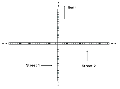
Figure 1: Two perpendicular closed chains representing the intersection of two uni directional traffic flows.

The system configuration at each time $t$ is characterized by specifying the occupation numbers $n_{i}$ and $m_{i}$ ($i=1,\cdots,L$) in both chains. The system dynamics is asymmetric simple exclusion process (ASEP). Although this choice is far from the realistic vehicular dynamics, we expect the general features of the problem namely the phase structure does not qualitative change. In addition, employing ASEP dynamics allows us to treat the problem more easily on analytical grounds. In reality, each driver yields to perpendicular traffic flow by appropriately adjusting of her velocity. In our formulation, this cautionary behaviour can be described by simple exclusion process. This process is defined as follows. During an infinitesimal time $dt$ each particle can stochastically hop to its forward neighbouring site provided the target site is empty. If the target site is already occupied by another particle, the attempted movement is rejected. At each time $t$, we define the particle approaching to the intersection as the one occupying the previous site $i=\frac{L}{2}-1$. We note that this particle’s attempt is successful if both sites $i_{1}=\frac{L}{2}$ and $i_{2}=\frac{L}{2}$ which is actually the common intersection site on both chains is empty. In terms of ASEP terminology, the sites $\frac{L}{2}-1$ can be regarded as dynamic impurity sites for each chain. The hoping rate at all sites are scaled to unity except at $i_{1}=\frac{L}{2}-1$ and $i_{2}=\frac{L}{2}-1$ which are $1-m_{\frac{L}{2}}$ and $1-n_{\frac{L}{2}}$ respectively.

II.1 Mean field approach

Let us denote the mean density at site $i$ and time $t$ of the first and second chains by $\langle n_{i}\rangle$ and $\langle m_{i}\rangle$ respectively. The master equation governing their time evolution can simply be written as follows:

$$\frac{d}{dt}\langle n_{i}\rangle=\langle n_{i-1}(1-n_{i})\rangle-\langle n_{i}(1-n_{i+1})\rangle~{}~{}$$ (1)

In the above equation, the site index $i$ covers all the lattice sites except $i=\frac{L}{2}-1$ and $i=\frac{L}{2}$. The rate equation for the second chain can be obtained by replacing $n_{i}$ by $m_{i}$. For sites $i=\frac{L}{2}-1$ and $i=\frac{L}{2}$, the rate equations have the following forms:

$$\frac{d}{dt}\langle n_{\frac{L}{2}-1}\rangle=\langle n_{\frac{L}{2}-2}(1-n_{\frac{L}{2}-1})\rangle-\langle n_{\frac{L}{2}-1}(1-n_{\frac{L}{2}}-m_{\frac{L}{2}})\rangle$$ (2)

$$\frac{d}{dt}\langle n_{\frac{L}{2}}\rangle=\langle n_{\frac{L}{2}-1}(1-n_{\frac{L}{2}}-m_{\frac{L}{2}})\rangle-\langle n_{\frac{L}{2}}(1-n_{\frac{L}{2}+1})\rangle$$ (3)

Similarly, the rate equations for $m_{\frac{L}{2}-1}$ and $m_{\frac{L}{2}}$ can be obtained by replacing $m\leftrightarrow n$ respectively. In order to proceed analytically we take into account the mean-field approximation. In this approximation, we replace the two-point functions by the product of one-point functions and furthermore we replace the probability that the middle site $i=\frac{L}{2}$ is empty, i.e. $(1-n_{\frac{L}{2}}-m_{\frac{L}{2}})$, by $(1-n_{\frac{L}{2}})(1-m_{\frac{L}{2}})$. The latter expression is the probability that the middle sites in each chain are simultaneously empty. In the steady state, the left hand sides of mean-field equations become zero and we arrive at a set of $2L$ nonlinear equations. Even by employing the assumption of mean field, we are not able to solve these nonlinear algebraic equations. Therefore, we should resort to numerical methods. We now outline a numerical approach for solving the set of nonlinear equations.

II.2 Numerical approach to mean field equations

Our approach for solving the MF equations is based on the constant density scheme which has originally been introduced by Barma and Tripathy barma1 ; barma2 . In this scheme, we first fix the global densities in two chains at given values $\rho_{1}$ and $\rho_{2}$. Second, we assign initial density profiles $n_{1}[0],n_{2}[0],\cdots,n_{L}[0]$ and $m_{1}[0],m_{2}[0],\cdots,m_{L}[0]$ to the first and second chain respectively. The constancy of global densities implies the following constraints on the initial profiles:

$$n_{1}[0]+n_{2}[0]+\cdots+n_{L}[0]=L\rho_{1}$$ (4)

$$m_{1}[0]+m_{2}[0]+\cdots+m_{L}[0]=L\rho_{2}$$ (5)

We next evolve the site densities according the following discrete time updating rules:

$$n_{i}[t+1]=n_{i}[t]+n_{i-1}[t](1-n_{i}[t])-n_{i}[t](1-n_{i+1}[t])$$ (6)

Similar equations hold for $m_{i}$. Note that in the above equations, $i$ covers the whole chain except the sites $i=\frac{L}{2}-1$ and $i=\frac{L}{2}$. The above discrete time evolution rules stem in time discretisation of the mean-field equations within Euler algorithm. In the special sites $i=\frac{L}{2}-1,\frac{L}{2}$ the interaction between two chains modifies the rate equations and we should take into account equations (2,3) which gives rise to the following dynamical rules:

$$n_{\frac{L}{2}-1}[t+1]=n_{\frac{L}{2}-1}[t]+n_{\frac{L}{2}-2}[t](1-n_{\frac{L}{2}-1}[t])-$$

$$n_{\frac{L}{2}-1}[t](1-n_{\frac{L}{2}}[t])(1-m_{\frac{L}{2}}[t])$$ (7)

$$n_{\frac{L}{2}}[t+1]=n_{\frac{L}{2}}[t]+n_{\frac{L}{2}-1}[t](1-n_{\frac{L}{2}}[t])(1-m_{\frac{L}{2}}[t])-$$

$$n_{\frac{L}{2}}[t](1-n_{\frac{L}{2}+1}[t])$$ (8)

The equations for $m_{\frac{L}{2}-1}$ and $m_{\frac{L}{2}}$ are simply obtained from the above equations via replacing $m$ by $n$ and vice versa. Notice that our dynamical equations preserve the constancy of global densities. More concisely, we have $n_{1}[t]+n_{2}[t]+\cdots+n_{L}[t]=L\rho_{1}$ and $m_{1}[t]+m_{2}[t]+\cdots+m_{L}[t]=L\rho_{2}$ at each $t$.

With an appropriate choice of initial condition, after iterating the above equations for many time steps the system is expected to reach a fixed point denoted by $\{n_{i}^{*}\}$ and $\{m_{i}^{*}\}$ in which further iteration does not change the densities. This solution can be considered as the solution of the mean-field equations. Note that in a acceptable solution, all the densities $n_{1}^{*},\cdots,n_{L}^{*}$ and $m_{1}^{*},\cdots,m_{L}^{*}$ should lie between zero and one. The chains currents are thus obtained according to the relations $J_{1}=n_{i}^{*}(1-n_{i+1}^{*})$ and $J_{2}=m_{i}^{*}(1-m_{i+1}^{*})$ in which $i$ can be any site of the chains. It should be noted that the choice of initial densities is a crucial step. Only certain initial condition converges to the desired solution. In general, the long-time behaviour of the density profile turns out to be an oscillatory pattern.

II.3 Monte Carlo simulation

For obtaining a better insight, we have also executed extensive Monte Carlo simulations which are presented in this section. The chains sizes are equally taken as $L_{1}=L_{2}=300$ and we averaged over 100 independent runs each of which with $10^{5}$ time steps per site. After transients, two chains maintain steady-state currents denoted by $J_{1}$ and $J_{2}$ which are function of the global densities $\rho_{1}$ and $\rho_{2}$. We kept the global density at a fixed value $\rho_{2}$ in the second chain and varied $\rho_{1}$. Figure (2) exhibits the fundamental diagram of the first chain.

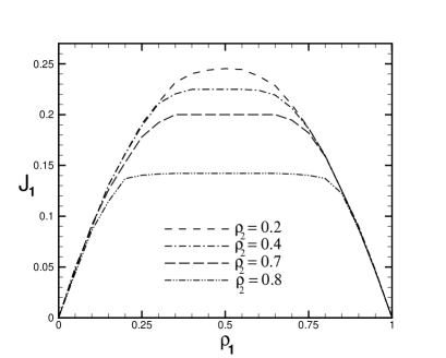
Figure 2: First chain current $J_{1}$ versus its density $\rho_{1}$ for various densities $\rho_{2}$ in the second chain. $L=300$.

The generic behaviour is reminiscent to ASEP with a single defective site lebowitz1 ; lebowitz2 ; barma2 . Intersection of two chains makes the intersection point appear as a dynamical defect. It is a well-known fact that a local defect can affect the system on a global scale lebowitz2 ; kolomeisky1 . This has been confirmed not only for simple exclusion process but also for cellular automata models, such as Nagel-Schreckenberg ns92 , describing vehicular traffic flow css99 ; chung ; yukawa . Analogous to static defects, in our case of dynamical impurity we observe that the effect of the dynamic defect is to form a plateau region $\rho\in[\rho_{-},\rho_{+}]$ in which $\rho_{\pm}=0.5\pm\Delta$ and $2\Delta$ is the extension of the plateau region in the fundamental diagram. In the plateau region the current is independent of the global density. The larger the density in the perpendicular chain is, the dynamic defect has larger strength. For higher $\rho_{2}$, the plateau region is wider and correspondingly the current value is more reduced. The notable point is that the flow capacity in the first chain persist to large decrease up to considerably large density $\rho_{2}\sim 0.5$ in the second chain. This marks the fact that conflicting flows of particles can, to a large extent, weakly affect each other. To shed some more light on this aspect, let us now consider the flow characteristics in the second chain. In figure (3) we sketch the behaviour of perpendicular fundamental diagram that is $J_{2}$ versus $\rho_{1}$.

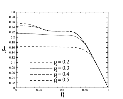
Figure 3: Second chain current $J_{2}$ versus density $\rho_{1}$ of the first chain for various densities $\rho_{2}$.

As depicted, $J_{2}$ shows a phase transition at the critical density $\rho_{1,c}=\rho_{+}$. Before $\rho_{1,c}$, the current exhibits smoothly decreasing behaviour. The nature of decrease depends on the value of $\rho_{2}$. For $\rho_{2}<0.3$ or $\rho_{2}>0.7$ $J_{2}$ is almost constant and is obtained from the single chain relation $J_{2}=\rho_{2}(1-\rho_{2})$. However, in the interval $0.3<\rho_{2}<0.7~{}$ $J_{2}$ shows a complex behaviour as is shown in figure (3). It first increases up to a small $\rho_{2}$ then smoothly diminishes until it reaches to a plateau region. The reason is due to interaction between two chains which induces correlations between them. This modifies the value of $J_{2}$ from the single chain value $\rho_{2}(1-\rho_{2})$. The appearance of a maximum in $J_{2}$ marks the point that a small density of cars in the first chain can even regulate the traffic, and hence enhance the flow, in the second chain. When the global density in the first chain exceeds the critical value, the perpendicular current exhibits a quasi linear decline. This corresponds to capacity break down in the second chain. In terminology of vehicular traffic, if the density of the perpendicular chain goes beyond a critical value, one should be warned that controlling of the traffic via self-organised mechanism starts to fail and traffic lights signalisation is thereby prescribed.

II.4 density profiles

In order to improve our understanding, it would be useful to look at the behaviour of density profiles in both chains. Let us look at some typical density profiles before attempting to give a general remark. The following figures, obtained by simulation, display the density profile in the first chain for two densities $\rho_{1}=0.2$ and $\rho_{1}=0.6$.

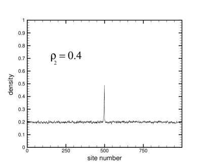
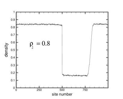
Figure 4: Density profile by MC simulation in the first chain: $\rho_{1}=0.2$ and $\rho_{2}=0.4$ (top) and $\rho_{1}=0.6$ and $\rho_{2}=0.8$ (bottom).

In figure (4) top, the second chain affects the first chain’s density profile only on a local scale. The reason is that the $\rho_{1}$ is below the limit to be globally affected. On the other hand, if one increases $\rho_{1}$ to a higher value e.g. $0.6$ (figure (4) bottom), it turns out that density profile of the first chain gives rise to segregation between a high and a low density regions. The formation of phase-segregated regime depends on the mutual values of global densities in both chains. The above observations have resemblance to the BML model of city traffic bml in the sense that below a given density, the conflicting flows do not affect each other much and the cars are not notably blocked by the other lane flow. Nevertheless, it should be mentioned that updating rules and road structures in the BML model are entirely different to our model’s. Furthermore, the blocking mechanism in the BML model is not only due to exclusion principle but is also related to the cooperative motion of vehicles. In our model, the it is only the exclusion at the crossing point which gives rise to blocking. To support our density profiles findings, which have been obtained by Monte Carlo simulations, we have numerically solved the mean-field equation in the constant-density scheme described in section II.B. The results are satisfactory and in qualitative agreement with Monte Carlo simulations. As an example, in figure (5) we have sketched and compared the profile of density in chain one for given global densities in both chain both with Monte Carlo and numerical mean field approach.

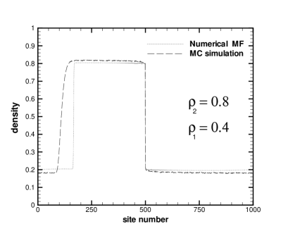
Figure 5: Density profile in the first chain obtained via MC (dashed) and MF (dotted). $\rho_{1}=0.4$ and $\rho_{2}=0.8$.

We observe that numerical mean field has qualitatively reproduced the phase-segregated behaviour. The difference between high and low densities given by MC and MF are in fairly well agreement. However, there is a notable difference in the vicinity of the domain wall. The prediction of MF is much sharper than that of MC. The more smooth transition from low to high density in MC is related to involve fluctuations which are not captured by the MF approach especially in low dimensions. In figure (6) we show density profiles in uniform phases.

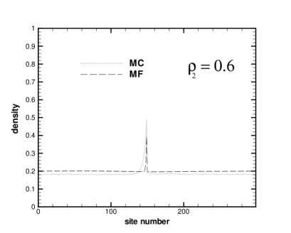
Figure 6: Density profile in the first chain obtained via MC and MF. $\rho_{1}=0.2$ and $\rho_{2}=0.6$. Number of iterations is $2000$.

The predictions of MF and MC are reasonably close to each other. Some comments on the constant-density approach seems unavoidable. In each iterative scheme, the stability of long time behaviour should be investigated. In our case, the choice of initial values of density profiles play an important role. We took their values within a small interval of size $\eta$ around the corresponding global densities. In figure (6) we set $\eta=0.01$. We note that the long time behaviour of the system of equations give rise to an oscillatory pattern of profile. In numerical terms, the iteration becomes unstable for large times. However, in intermediate times, iterative method gives a reasonable answer. In figure (7) we have depicted the behaviour of the density profiles for a larger iteration. We have varied the the number of iterations $M$ for $2000,5000$ and $10000$ (from bottom to top) correspondingly. For clarity, densities are shifted upwards for $M=5000$ and $M=10000$.

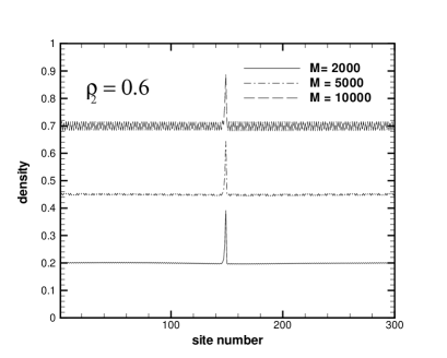
Figure 7: Density profile in the first chain obtained via numerical MF. $\rho_{1}=0.2$ and $\rho_{2}=0.6$.

We now turn into the general behaviour of density profiles. It would be a natural question to ask under what circumstance yielding leads to traffic jam formation in the first chain before the crossing point. To this end, by Monte Carlo simulations we have systematically surveyed the entire phase space $\rho_{1}-\rho_{2}$ in the grids of $\delta\rho=0.05$ . Two phases are identified: uniform (homogeneous) and phase-segregated. In the uniform phase, the interaction between two chains has only a local effect on profile of the first chain whereas in the segregated phase, a domain wall separates a low density and a high density region. Figure (8) exhibits the phase structure of the problem. By symmetry, one obtains the phase structure of the second chain via replacing $1\leftrightarrow 2$.

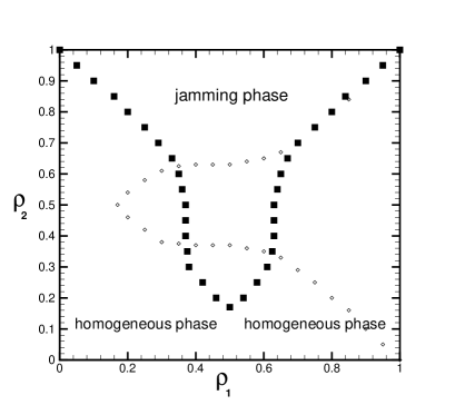
Figure 8: Phase diagram of the model for the first chain. $\diamond$ shows the corresponding diagram for the second chain.

III Mean-field phase diagram: Analytical approach

Here we try to outline an analytical approach to obtain the model phase diagram. This approach is based on the concept of density phase segregation proposed in lebowitz1 ; lebowitz2 . Suppose for given densities $\rho_{1}$ and $\rho_{2}$ one has density phase segregation in both chains. We denote the high and low densities in the first chain by by $\rho_{h}$ and $\rho_{l}$ and in the second chain by $\xi_{h}$ and $\xi_{l}$ respectively. Also let us denote the relative length of low and high density regions in the first chain by $a_{l}$ and $a_{h}$ and in the second chain by $b_{l}$ and $b_{h}$. We denote the probability of occupation of the crossing site by a car from the first (second) chain by $r_{1}~{}(r_{2}$). Therefore the probability that the crossing site will be empty is $1-r_{1}-r_{2}$. We can write the following mean field equations:

$$J_{1}=\rho_{l}(1-\rho_{l});~{}~{}~{}~{}~{}J_{2}=\xi_{l}(1-\xi_{l}).$$ (9)

$$J_{1}=\rho_{h}(1-\rho_{h});~{}~{}~{}~{}~{}J_{2}=\xi_{h}(1-\xi_{h})$$ (10)

$$J_{1}=\rho_{h}(1-r_{1}-r_{2});~{}~{}~{}~{}J_{2}=\xi_{h}(1-r_{1}-r_{2})$$ (11)

$$J_{1}=r_{1}(1-\rho_{l});~{}~{}~{}~{}J_{2}=r_{2}(1-\xi_{l})$$ (12)

$$a_{l}+a_{h}=1;~{}~{}~{}~{}~{}b_{l}+b_{h}=1$$ (13)

$$\rho_{l}a_{l}+\rho_{h}a_{h}=\rho_{1};~{}~{}~{}~{}\xi_{l}b_{l}+\xi_{h}b_{h}=\rho_{2}$$ (14)

The above equations are easily solved and we find:

$$r_{1}=r_{2}=\frac{1}{3};~{}\rho_{l}=\xi_{l}=\frac{1}{3};~{}\rho_{h}=\xi_{h}=\frac{2}{3};~{}J_{1}=J_{2}=\frac{2}{9}$$ (15)

One also finds: $a_{l}=2-3\rho_{1}$ and $b_{l}=2-3\rho_{2}$. The conditions $0\leq a_{l}\leq 1$ and $0\leq b_{l}\leq 1$ imply: $\frac{1}{3}\leq\rho_{1},\rho_{2}\leq\frac{2}{3}$. In figure (9), we have plotted the phase diagram. In the interior region, one has density phase segregation in both streets. We note that middle square region is in well qualitative agreement with the prediction of MC simulations ( intersection of two curves in fig8 ).

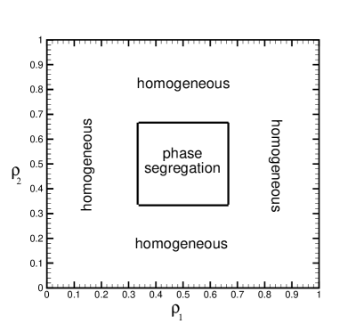
Figure 9: Phase diagram of the model.

IV Summary and Concluding Remarks

We have investigated the characteristics of two conflicting traffic flows within the framework of asymmetric simple exclusion process. Two perpendicular chains interact with each other via the intersection point. Using Monte Carlo simulations and numerics, we have obtained the dependence of each chain current on its own and on its perpendicular chain global density. It is verified that the chains can maintain large currents up to rather a high density. Interaction of two chains can effectively be considered as a dynamic impurity. For some values of global densities in the chains, the interaction of chains leads to formation of high density region behind the intersection point which is segregated from a low density region afterwards. By a systematic scanning of the phase space, we have obtained the structure of model phase diagram. Two phases of jamming (density segregated) and regulated (uniform density) flows are identified.

V acknowledgement

Fruitful discussions with Mustansir Barma, Gunter Schütz, David Mukamel and Anatoly Kolomeisky are appreciated. Special thanks are given to Majid Arabgol and Soltaan Abdol Hossein for useful helps.

References

- [1] B. Schmittmann and R.K.P. Zia in: Phase transitions and Crtitical Phenomena, vol 17, ed. C. Domb and L. Lebowitz (London: Academic) 1995.
- [2] G. Schütz in: Phase transitions and Crtitical Phenomena, vol 19, ed. C. Domb and L. Lebowitz, Academic Press, 2001.
- [3] B. Kerner, in Physics of traffic flow, Springer, 2004.
- [4] D. Chowdhury, L. Santen and A. Schadschneider, Physics Reports, 329, 199 (2000).
- [5] D. Helbing, Rev. Mod. Phys., 73, 1067 (2001).
- [6] O. Biham, A. Middleton and D. Levine, Phys.Rev. A 46, R6124 (1992).
- [7] T. Nagatani, Phys. Rev. E 48, 3290 (1993).
- [8] D. Chowdhury and A. Schadschneider, Phys. Rev. E 59, R 1311 (1999).
- [9] M.E. Fouladvand and M. Nematollahi, Eur. Phys. J. B 22, 395 (2001).
- [10] M.E. Fouladvand, Z. Sadjadi and M.R. Shaebani J. Phys. A: Math. Gen, 37, 561 (2004).
- [11] M.E. Fouladvand, Z. Sadjadi and M.R. Shaebani Phys. Rev. E, 70, 046132 (2004).
- [12] B. Ray and S.N. Bhattacharyya, Phys. Rev. E, 73, 036101 (2006).
- [13] C. Rui-Xiong, Bai Ke- Zhao and L Mu-Ren, Chinese Physics, 15, No 7, July 2006.
- [14] S-B Cools, C. Gershenson and B. D Hooghe, arXive: nlin.AO/0610040
- [15] M.E. Foulaadvand and S. Belbaasi, J. Phys. A: Math. Theor., 40, 8289 (2007).
- [16] J.T. MacDonald, J.H. Gibbs and A.C. Pipkin Biopolymers, 6, 1 (1968).
- [17] B. Derrida, M.R. Evans, V. Hakim and V. Pasquir J. Phys. A, 26, 1493 (1993).
- [18] B. Derrida Physics Report, 301, 65 (1998).
- [19] S. Janowsky and J. Lebowitz Phys. Rev. A, 45, 618 (1992).
- [20] S. Janowsky and J. Lebowitz J. Stat. Phys., 77, 35 (1994).
- [21] A.B. Kolomeisky, J. Phys. A: Math, Gen., 31, 1153 (1998).
- [22] M.R. Evans, J. Phys. A: Math,Gen., 30, 5669 (1997).
- [23] T. Chou and G. Lakatos, Phys. Rev. Lett., 93, 198101 (2004).
- [24] G. Lakatos, T. Chou and A.B. Kolomeisky, Phys. Rev. E, 71, 011103 (2005).
- [25] M.E. Foulaadvand, S. Chaaboki and M. Saalehi Phys. Rev. E, 75, 011127 (2007).
- [26] E. Ekaterina and A. B. Kolomeisky, J. Stat. Mech., 07, P07010. (2005).
- [27] G. Tripathy and M. Barma, Phys. Rev. Lett., 78, 3039 (1997).
- [28] G. Tripathy and M. Barma, Phys. Rev. E, 58, 1911 (1998).
- [29] K. Nagel, M. Schreckenberg, J. Phys. I France 2, 2221 (1992).
- [30] K.H. Chung and P.M. Hui, J. Phys. Soc. Jap., 63, 4338 (1994).
- [31] S. Yukawa, M. Kikuchi and S. Tadaki J. Phys. Soc. Jap., 63, 3609 (1994).