Novel Bounds on Marginal Probabilities

Abstract

We derive two related novel bounds on single-variable marginal probability distributions in factor graphs with discrete variables. The first method propagates bounds over a subtree of the factor graph rooted in the variable, and the second method propagates bounds over the self-avoiding walk tree starting at the variable. By construction, both methods not only bound the exact marginal probability distribution of a variable, but also its approximate Belief Propagation marginal (“belief”). Thus, apart from providing a practical means to calculate bounds on marginals, our contribution also lies in an increased understanding of the error made by Belief Propagation. Empirically, we show that our bounds often outperform existing bounds in terms of accuracy and/or computation time. We also show that our bounds can yield nontrivial results for medical diagnosis inference problems.

Keywords: Graphical Models, Factor Graphs, Inference, Marginal Probability Distributions, Bounds

1 Introduction

Graphical models are used in many different fields. A fundamental problem in the application of graphical models is that exact inference is NP-hard (Cooper, 1990). In recent years, much research has focused on approximate inference techniques, such as sampling methods and deterministic approximation methods, e.g., Belief Propagation (BP) (Pearl, 1988). Although the approximations obtained by these methods can be very accurate, there are only few guarantees on the error of the approximation, and often it is not known (without comparing with the exact solution) how accurate an approximate result is. Thus it is desirable to calculate, in addition to the approximate results, tight bounds on the approximation error. Existing methods to calculate bounds on marginals include (Tatikonda, 2003; Leisink and Kappen, 2003; Taga and Mase, 2006; Ihler, 2007). Also, upper bounds on the partition sum, e.g., (Jaakkola and Jordan, 1996; Wainwright et al., 2005), can be combined with lower bounds on the partition sum, such as the well-known mean field bound or higher-order lower bounds (Leisink and Kappen, 2001), to obtain bounds on marginals.

In this article, we derive novel bounds on exact single-variable marginals in factor graphs. The original motivation for this work was to better understand and quantify the BP error. This has lead to bounds which are at the same time bounds for the exact single-variable marginals as well as for the BP beliefs. A particularly nice feature of the bounds is that their computational cost is relatively low, provided that the number of possible values of each variable in the factor graph is small. Unfortunately, the computation time is exponential in the number of possible values of the variables, which limits application to factor graphs in which each variable has a low number of possible values. On these factor graphs however, our bounds perform exceedingly well and we show empirically that they outperform the state-of-the-art in a variety of factor graphs, including real-world problems arising in medical diagnosis.

This article is organized as follows. In the next section, we derive our novel bounds. In Section 3, we discuss related work. In Section 4 we present experimental results. We conclude with conclusions and a discussion in Section 5.

2 Theory

In this work, we consider graphical models such as Markov random fields and Bayesian networks. We use the unifying factor graph representation (Kschischang et al., 2001). In the first subsection, we introduce our notation and some basic definitions concerning factor graphs. Then, we shortly remind the reader of some basic facts about convexity. After that, we introduce some notation and concepts for measures on subsets of variables. We proceed with a subsection that considers the interplay between convexity and the operations of normalization and multiplication. In the next subsection, we introduce “(smallest bounding) boxes” that will be used to describe sets of measures in a convenient way. Then, we formulate the basic lemma that will be used to obtain bounds on marginals. We illustrate the basic lemma with two simple examples. Then we formulate our first result, an algorithm for propagating boxes over a subtree of the factor graph, which results in a bound on the marginal of the root variable of the subtree. In the last subsection, we show how one can go deeper into the computation tree and derive our second result, an algorithm for propagating boxes over self-avoiding walk trees. The result of that algorithm is a bound on the marginal of the root variable (starting point) of the self-avoiding walk tree. For the special case where all factors in the factor graph depend on two variables at most (“pairwise interactions”), our first result is equivalent to a truncation of the second one. This is not true for higher-order interactions, however.

2.1 Factor graphs

Let $\mathcal{V}:=\{1,\dots,N\}$ and consider $N$ discrete random variables $(x_{i})_{i\in\mathcal{V}}$. Each variable $x_{i}$ takes values in a discrete domain $\mathcal{X}_{i}$. We will frequently use the following multi-index notation. Let $A=\{i_{1},i_{2},\dots,i_{m}\}\subseteq\mathcal{V}$ with $i_{1}<i_{2}<\dots i_{m}$. We write $\mathcal{X}_{A}:=\mathcal{X}_{i_{1}}\times\mathcal{X}_{i_{2}}\times\dots\times\mathcal{X}_{i_{m}}$ and for any family $(Y_{i})_{i\in B}$ with $A\subseteq B\subseteq\mathcal{V}$, we write $Y_{A}:=(Y_{i_{1}},Y_{i_{2}},\dots,Y_{i_{m}})$.

We consider a probability distribution over $x=(x_{1},\dots,x_{N})\in\mathcal{X}_{\mathcal{V}}$ that can be written as a product of factors (also called “interactions”) $(\psi_{I})_{I\in\mathcal{F}}$:

$$\mathbb{P}(x)=\frac{1}{Z}\prod_{I\in\mathcal{F}}\psi_{I}(x_{N_{I}}),\qquad Z=\sum_{x\in\mathcal{X}_{\mathcal{V}}}\prod_{I\in\mathcal{F}}\psi_{I}(x_{N_{I}}).$$ (1)

For each factor index $I\in\mathcal{F}$, there is an associated subset $N_{I}\subseteq\mathcal{V}$ of variable indices and the factor $\psi_{I}$ is a nonnegative function $\psi_{I}:\mathcal{X}_{N_{I}}\to[0,\infty)$. For a Bayesian network, the factors are (conditional) probability tables. In case of Markov random fields, the factors are often called potentials. In the following, we will use lowercase for variable indices and uppercase for factor indices.

In general, the normalizing constant $Z$ is not known and exact computation of $Z$ is infeasible, due to the fact that the number of terms to be summed is exponential in $N$. Similarly, computing marginal distributions $\mathbb{P}(x_{A})$ for subsets of variables $A\subseteq\mathcal{V}$ is intractable in general. In this article, we focus on the task of obtaining rigorous bounds on single-variable marginals $\mathbb{P}(x_{i})=\sum_{x_{\mathcal{V}\setminus\{i\}}}\mathbb{P}(x)$.

We can represent the structure of the probability distribution (1) using a factor graph $(\mathcal{V},\mathcal{F},\mathcal{E})$. This is a bipartite graph, consisting of variable nodes $i\in\mathcal{V}$, factor nodes $I\in\mathcal{F}$, and edges $e\in\mathcal{E}$, with an edge $\{i,I\}$ between $i\in\mathcal{V}$ and $I\in\mathcal{F}$ if and only if the factor $\psi_{I}$ depends on $x_{i}$ (i.e., if $i\in N_{I}$). We will represent factor nodes visually as rectangles and variable nodes as circles. Figure 1 shows a simple example of a factor graph and the corresponding probability distribution. The set of neighbors of a factor node $I$ is precisely $N_{I}$; similarly, we denote the set of neighbors of a variable node $i$ by $N_{i}:=\{I\in\mathcal{F}:i\in N_{I}\}$. Further, we define for each variable $i\in\mathcal{V}$ the set ${\Delta{i}}:=\bigcup N_{i}$ consisting of all variables that appear in some factor in which variable $i$ participates, and the set ${\partial{i}}:={\Delta{i}}\setminus\{i\}$, the Markov blanket of $i$.

Figure 1: Example of a factor graph with three variable nodes ($i,j,k$), represented as circles, and three factor nodes ($J,K,L$), represented as rectangles. The corresponding random variables are $x_{i},x_{j},x_{k}$; the corresponding factors are $\psi_{J}:\mathcal{X}_{i}\times\mathcal{X}_{j}\to[0,\infty)$, $\psi_{K}:\mathcal{X}_{i}\times\mathcal{X}_{k}\to[0,\infty)$ and $\psi_{L}:\mathcal{X}_{j}\times\mathcal{X}_{k}\to[0,\infty)$. The corresponding probability distribution $\mathbb{P}(x)$ is written out on the right.

We will assume throughout this article that the factor graph corresponding to (1) is connected. Furthermore, we will assume that

$$\forall{I\in\mathcal{F}}\ \forall{i\in N_{I}}\ \forall{x_{N_{I}\setminus\{i\}}\in\mathcal{X}_{N_{I}\setminus\{i\}}}:\sum_{x_{i}\in\mathcal{X}_{i}}\psi_{I}(x_{i},x_{N_{I}\setminus\{i\}})>0.$$

This will prevent technical problems regarding normalization later on.

One final remark concerning notation: we will sometimes abbreviate $\{i\}$ as $i$ if no confusion can arise.

2.2 Convexity

Let $V$ be a real vector space. For $T$ elements $(v_{t})_{t=1,\dots,T}$ of $V$ and $T$ nonnegative numbers $(\lambda_{t})_{t=1,\dots,T}$ with $\sum_{t=1}^{T}\lambda_{t}=1$, we call $\sum_{t=1}^{T}\lambda_{t}v_{t}$ a convex combination of the $(v_{t})_{t=1,\dots,T}$ with weights $(\lambda_{t})_{t=1,\dots,T}$. A subset $X\subseteq V$ is called convex if for all $x_{1},x_{2}\in X$ and all $\lambda\in[0,1]$, the convex combination $\lambda x_{1}+(1-\lambda)x_{2}\in X$. An extreme point of a convex set $X$ is an element $x\in X$ which cannot be written as a (nontrivial) convex combination of two different points in $X$. In other words, $x\in X$ is an extreme point of $X$ if and only if for all $\lambda\in(0,1)$ and all $x_{1},x_{2}\in X$, $x=\lambda x_{1}+(1-\lambda)x_{2}$ implies $x_{1}=x_{2}$. We denote the set of extreme points of a convex set $X$ by $\mathrm{Ext}\,(X)$. For a subset $Y$ of the vector space $V$, we define the convex hull of $Y$ to be the smallest convex set $X\subseteq V$ with $Y\subseteq X$; we denote the convex hull of $Y$ as $\mathrm{Hull}\,(Y)$.

2.3 Measures and operators

For $A\subseteq\mathcal{V}$, define $\mathcal{M}_{A}:=[0,\infty)^{\mathcal{X}_{A}}$, i.e., $\mathcal{M}_{A}$ is the set of nonnegative functions on $\mathcal{X}_{A}$. $\mathcal{M}_{A}$ can be identified with the set of finite measures on $\mathcal{X}_{A}$. We will simply call the elements of $\mathcal{M}_{A}$ “measures on $A$”. We also define $\mathcal{M}_{A}^{*}:=\mathcal{M}_{A}\setminus\{0\}$. We will denote $\mathcal{M}:=\bigcup_{A\subseteq\mathcal{V}}\mathcal{M}_{A}$ and $\mathcal{M}^{*}:=\bigcup_{A\subseteq\mathcal{V}}\mathcal{M}_{A}^{*}$.

Adding two measures $\Psi,\Phi\in\mathcal{M}_{A}$ results in the measure $\Psi+\Phi$ in $\mathcal{M}_{A}$. For $A,B\subseteq\mathcal{V}$, we can multiply an element of $\mathcal{M}_{A}$ with an element of $\mathcal{M}_{B}$ to obtain an element of $\mathcal{M}_{A\cup B}$; a special case is multiplication with a scalar. Note that there is a natural embedding of $\mathcal{M}_{A}$ in $\mathcal{M}_{B}$ for $A\subseteq B\subseteq\mathcal{V}$ obtained by multiplying an element $\Psi\in\mathcal{M}_{A}$ by $\mathbf{1}_{B\setminus A}\in\mathcal{M}_{B\setminus A}$, the constant function with value 1 on $\mathcal{X}_{B\setminus A}$. Another important operation is the partial summation: given $A\subseteq B\subseteq\mathcal{V}$ and $\Psi\in\mathcal{M}_{B}$, define $\sum_{x_{A}}\Psi$ to be the measure in $\mathcal{M}_{B\setminus A}$ that satisfies

$$\left(\sum_{x_{A}}\Psi\right)(x_{B\setminus A})=\sum_{x_{A}\in\mathcal{X}_{A}}\Psi(x_{A},x_{B\setminus A})\qquad\forall x_{B\setminus A}\in\mathcal{X}_{B\setminus A}.$$

Also, defining $A^{\prime}=B\setminus A$, we will sometimes write this measure as $\sum_{x_{\setminus A^{\prime}}}\Psi$, which is an abbreviation of $\sum_{x_{B\setminus A^{\prime}}}\Psi$. This notation does not make explicit which variables are summed over (which depends on the measure that is being partially summed), although it shows which variables remain after summation.

In the following, we will implicitly define operations on sets of measures by applying the operation on elements of these sets and taking the set of the resulting measures; e.g., if we have two subsets $\Xi_{A}\subseteq\mathcal{M}_{A}$ and $\Xi_{B}\subseteq\mathcal{M}_{B}$ for $A,B\subseteq\mathcal{V}$, we define the product of the sets $\Xi_{A}$ and $\Xi_{B}$ to be the set of the products of elements of $\Xi_{A}$ and $\Xi_{B}$, i.e., $\Xi_{A}\Xi_{B}:=\{\Psi_{A}\Psi_{B}:\Psi_{A}\in\Xi_{A},\Psi_{B}\in\Xi_{B}\}$.

In Figure 2, the simple case of a binary random variable $x_{i}$ and the subset $A=\{i\}$ is illustrated. Note that in this case, a measure $\Psi\in\mathcal{M}_{i}$ can be identified with a point in the quarter plane $[0,\infty)\times[0,\infty)$.

Figure 2: Illustration of some concepts in the simple case of a binary random variable $x_{i}\in\mathcal{X}_{i}=\{\pm 1\}$ and the subset $A=\{i\}$. A measure $\Psi\in\mathcal{M}_{i}$ can be identified with a point in the quarter plane as indicated in the Figure. A normalized measure can be obtained by scaling $\Psi$; the result $\mathcal{N}\Psi$ is contained in the simplex $\mathcal{P}_{i}$, a lower-dimensional submanifold of $\mathcal{M}_{i}$.

We will define $\mathcal{Q}_{A}$ to be the set of completely factorized measures on $A$, i.e.,

$$\mathcal{Q}_{A}:=\prod_{a\in A}\mathcal{M}_{\{a\}}=\left\{\prod_{a\in A}\Psi_{a}:\Psi_{a}\in\mathcal{M}_{\{a\}}\text{ for each }a\in A\right\}.$$

Note that $\mathcal{M}_{A}$ is the convex hull of $\mathcal{Q}_{A}$. Indeed, we can write each measure $\Psi\in\mathcal{M}_{A}$ as a convex combination of measures in $\mathcal{Q}_{A}$; let $Z:=\sum_{x_{A}}\Psi$ and note that

$$\Psi(x)=\sum_{y\in\mathcal{X}_{A}}\frac{\Psi(y)}{Z}\left(Z\delta_{y}(x)\right)\qquad\forall x\in\mathcal{X}_{A}.$$

For any $y\in\mathcal{X}_{A}$, the Kronecker delta function $\delta_{y}\in\mathcal{M}_{A}$ (which is 1 if its argument is equal to $y$ and 0 otherwise) is an element of $\mathcal{Q}_{A}$ because $\delta_{y}(x)=\prod_{a\in A}\delta_{y_{a}}(x_{a})$. We denote $\mathcal{Q}_{A}^{*}:=\mathcal{Q}_{A}\setminus\{0\}$.

We define the partition sum operator $\mathcal{Z}:\mathcal{M}\to[0,\infty)$ which calculates the partition sum (normalization constant) of a measure, i.e.,

$$\mathcal{Z}\Psi:=\sum_{x_{A}\in\mathcal{X}_{A}}\Psi(x_{A})\qquad\text{for $\Psi\in\mathcal{M}_{A}$, $A\subseteq\mathcal{V}$}.$$

We denote with $\mathcal{P}_{A}$ the set of probability measures on $A$, i.e., $\mathcal{P}_{A}=\{\Psi\in\mathcal{M}_{A}:\mathcal{Z}\Psi=1\}$, and define $\mathcal{P}:=\bigcup_{A\subseteq\mathcal{V}}\mathcal{P}_{A}$. The set $\mathcal{P}_{A}$ is called a simplex (see also Figure 2). Note that a simplex is convex; the simplex $\mathcal{P}_{A}$ has precisely $\#(\mathcal{X}_{A})$ extreme points, each of which corresponds to putting all probability mass on one of the possible values of $x_{A}$.

Define the normalization operator $\mathcal{N}:\mathcal{M}^{*}\to\mathcal{P}$ which normalizes a measure, i.e.,

$$\mathcal{N}\Psi:=\frac{1}{\mathcal{Z}\Psi}\Psi\qquad\text{for $\Psi\in\mathcal{M}^{*}$}.$$

Note that $\mathcal{Z}\circ\mathcal{N}=1$. Figure 2 illustrates the normalization of a measure in a simple case.

2.4 Convex sets of measures

To calculate marginals of subsets of variables in some factor graph, several operations performed on measures are relevant: normalization, taking products of measures, and summing over subsets of variables. In this section we study the interplay between convexity and these operations; this will turn out to be useful later on, because our bounds make use of convex sets of measures that are propagated over the factor graph.

The interplay between normalization and convexity is described by the following Lemma, which is illustrated in Figure 3.

Figure 3: Any convex combination of $\mathcal{N}\xi_{1}$, $\mathcal{N}\xi_{2}$ and $\mathcal{N}\xi_{3}$ can be written as a normalized convex combination of $\xi_{1}$, $\xi_{2}$ and $\xi_{3}$. Vice versa, normalizing a convex combination of $\xi_{1},\xi_{2}$ and $\xi_{3}$ yields a convex combination of $\mathcal{N}\xi_{1},\mathcal{N}\xi_{2}$ and $\mathcal{N}\xi_{3}$.

Lemma 1

Let $A\subseteq\mathcal{V}$, $T\in\mathbb{N}^{*}$ and let $(\xi_{t})_{t=1,\dots,T}$ be elements of $\mathcal{M}_{A}^{*}$. Each convex combination of the normalized measures $(\mathcal{N}\xi_{t})_{t=1,\dots,T}$ can be written as a normalized convex combination of the measures $(\xi_{t})_{t=1,\dots,T}$ (which has different weights in general), and vice versa.

Proof  Let $(\lambda_{t})_{t=1,\dots,T}$ be nonnegative numbers with $\sum_{t=1}^{T}\lambda_{t}=1$. Then

$$\mathcal{Z}\left(\sum_{t=1}^{T}\lambda_{t}\mathcal{N}\xi_{t}\right)=\sum_{t=1}^{T}\lambda_{t}\mathcal{Z}\mathcal{N}\xi_{t}=1,$$

therefore

$$\sum_{t=1}^{T}\lambda_{t}(\mathcal{N}\xi_{t})=\mathcal{N}\left(\sum_{t=1}^{T}\lambda_{t}(\mathcal{N}\xi_{t})\right)=\mathcal{N}\left(\sum_{t=1}^{T}\frac{\lambda_{t}}{\mathcal{Z}\xi_{t}}\xi_{t}\right)=\mathcal{N}\left(\sum_{t=1}^{T}\frac{\frac{\lambda_{t}}{\mathcal{Z}\xi_{t}}}{\sum_{s=1}^{T}\frac{\lambda_{s}}{\mathcal{Z}\xi_{s}}}\ \xi_{t}\right),$$

which is the result of applying the normalization operator to a convex combination of the elements $(\xi_{t})_{t=1,\dots,T}$.

Vice versa, let $(\mu_{t})_{t=1,\dots,T}$ be nonnegative numbers with $\sum_{t=1}^{T}\mu_{t}=1$. Then

$$\mathcal{N}\left(\sum_{t=1}^{T}\mu_{t}\xi_{t}\right)=\sum_{t=1}^{T}\frac{\mu_{t}}{Z}\xi_{t}$$

where

$$Z:=\mathcal{Z}\left(\sum_{t=1}^{T}\mu_{t}\xi_{t}\right)=\sum_{t=1}^{T}\mu_{t}\mathcal{Z}\xi_{t}=\sum_{t=1}^{T}\mu_{t}Z_{t}$$

where we defined $Z_{t}:=\mathcal{Z}\xi_{t}$ for all $t=1,\dots,T$. Thus

$$\mathcal{N}\left(\sum_{t=1}^{T}\mu_{t}\xi_{t}\right)=\sum_{t=1}^{T}\frac{\mu_{t}}{\sum_{s=1}^{T}\mu_{s}Z_{s}}\xi_{t}=\sum_{t=1}^{T}\frac{\mu_{t}Z_{t}}{\sum_{s=1}^{T}\mu_{s}Z_{s}}\mathcal{N}\xi_{t},$$

which is a convex combination of the normalized measures $(\mathcal{N}\xi_{t})_{t=1,\dots,T}$.  

The following lemma concerns the interplay between convexity and taking products; it says that if we take the product of convex sets of measures on different spaces, the resulting set is contained in the convex hull of the product of the extreme points of the convex sets. We have not made a picture corresponding to this lemma because the simplest nontrivial case would require at least four dimensions.

Lemma 2

Let $T\in\mathbb{N}^{*}$ and $(A_{t})_{t=1,\dots,T}$ be a family of mutually disjoint subsets of $\mathcal{V}$. For each $t=1,\dots,T$, let $\Xi_{t}\subseteq\mathcal{M}_{A_{t}}$ be convex with a finite number of extreme points. Then:

$$\prod_{t=1}^{T}\Xi_{t}\subseteq\mathrm{Hull}\,\left(\prod_{t=1}^{T}\mathrm{Ext}\,\Xi_{t}\right),$$

Proof  Let $\Psi_{t}\in\Xi_{t}$ for each $t=1,\dots,T$. For each $t$, $\Psi_{t}$ can be written as a convex combination

$$\Psi_{t}=\sum_{\xi_{t}\in\mathrm{Ext}\,(\Xi_{t})}\lambda_{t;\xi_{t}}\xi_{t},\qquad\sum_{\xi_{t}\in\mathrm{Ext}\,(\Xi_{t})}\lambda_{t;\xi_{t}}=1,\qquad\forall\ {\xi_{t}\in\mathrm{Ext}\,(\Xi_{t})}:\lambda_{t;\xi_{t}}\geq 0.$$

Therefore the product $\prod_{t=1}^{T}\Psi_{t}$ is also a convex combination:

$$\prod_{t=1}^{T}\Psi_{t} =\prod_{t=1}^{T}\left(\sum_{\xi_{t}\in\mathrm{Ext}\,(\Xi_{t})}\lambda_{t;\xi_{t}}\xi_{t}\right)$$

$$=\sum_{\xi_{1}\in\mathrm{Ext}\,(\Xi_{1})}\sum_{\xi_{2}\in\mathrm{Ext}\,(\Xi_{2})}\dots\sum_{\xi_{T}\in\mathrm{Ext}\,(\Xi_{T})}\left(\prod_{t=1}^{T}\lambda_{t;\xi_{t}}\right)\left(\prod_{t=1}^{T}\xi_{t}\right)$$

$$\in\mathrm{Hull}\,\left(\prod_{t=1}^{T}\mathrm{Ext}\,\Xi_{t}\right).$$

 

2.5 Boxes and smallest bounding boxes

In this subsection, we define “(smallest bounding) boxes”, certain convex sets of measures that will play a central role in our bounds, and study some of their properties.

Definition 3

Let $A\subseteq\mathcal{V}$. For ${\underline{\Psi}}\in\mathcal{M}_{A}$ and ${\overline{\Psi}}\in\mathcal{M}_{A}$ with ${\underline{\Psi}}\leq{\overline{\Psi}}$, we define the box between the lower bound ${\underline{\Psi}}$ and the upper bound ${\overline{\Psi}}$ by

$$\mathcal{B}_{A}\left({\underline{\Psi}},{\overline{\Psi}}\right):=\{\Psi\in\mathcal{M}_{A}:{\underline{\Psi}}\leq\Psi\leq{\overline{\Psi}}\}.$$

The inequalities should be interpreted pointwise, e.g., ${\underline{\Psi}}\leq\Psi$ means ${\underline{\Psi}}(x)\leq\Psi(x)$ for all $x\in\mathcal{X}_{A}$. Note that a box is convex; indeed, its extreme points are the “corners” of which there are $2^{\#(\mathcal{X}_{A})}$.

Definition 4

Let $A\subseteq\mathcal{V}$ and $\Xi\subseteq\mathcal{M}_{A}$ be bounded (i.e., $\Xi\leq\Psi$ for some $\Psi\in\mathcal{M}_{A}$). The smallest bounding box for $\Xi$ is defined as $\mathcal{B}\left(\Xi\right):=\mathcal{B}_{A}\left({\underline{\Psi}},{\overline{\Psi}}\right)$, where ${\underline{\Psi}},{\overline{\Psi}}\in\mathcal{M}_{A}$ are given by

$$\begin{array}[]{lll}{\underline{\Psi}}(x_{A})&\!:=\inf\{\Psi(x_{A}):\Psi\in\Xi\}&\qquad\forall x_{a}\in\mathcal{X}_{A},\\ {\overline{\Psi}}(x_{A})&\!:=\sup\{\Psi(x_{A}):\Psi\in\Xi\}&\qquad\forall x_{a}\in\mathcal{X}_{A}.\end{array}$$

Figure 4 illustrates this concept. Note that $\mathcal{B}\left(\Xi\right)=\mathcal{B}\left(\mathrm{Hull}\,(\Xi)\right)$. Therefore, if $\Xi$ is convex, the smallest bounding box for $\Xi$ depends only on the extreme points $\mathrm{Ext}\,(\Xi)$, i.e., $\mathcal{B}\left(\Xi\right)=\mathcal{B}\left(\mathrm{Ext}\,(\Xi)\right)$.

Figure 4: The smallest bounding box $\mathcal{B}\left(\Xi\right)$ for $\Xi$ is given by the box $\mathcal{B}_{i}\left({\underline{\Psi}},{\overline{\Psi}}\right)$ with lower bound ${\underline{\Psi}}$ and upper bound ${\overline{\Psi}}$.

Figure 5: Multiplication of two boxes on the same variable set $A=\{i\}$.

The product of several boxes on the same subset $A$ of variables can be easily calculated as follows (see also Figure 5).

Lemma 5

Let $A\subseteq\mathcal{V}$, $T\in\mathbb{N}^{*}$ and for each $t=1,\dots,T$, let ${\underline{\Psi}}_{t},{\overline{\Psi}}_{t}\in\mathcal{M}_{A}$ such that ${\underline{\Psi}}_{t}\leq{\overline{\Psi}}_{t}$. Then

$$\prod_{t=1}^{T}\mathcal{B}_{A}\left({\underline{\Psi}}_{t},{\overline{\Psi}}_{t}\right)=\mathcal{B}_{A}\left(\prod_{t=1}^{T}{\underline{\Psi}}_{t},\prod_{t=1}^{T}{\overline{\Psi}}_{t}\right),$$

i.e., the product of the boxes is again a box, with as lower bound the product of the lower bounds of the boxes and as upper bound the product of the upper bounds of the boxes.

Proof  We prove the case $T=2$; the general case follows by induction. We show that

$$\mathcal{B}_{A}\left({\underline{\Psi}}_{1},{\overline{\Psi}}_{1}\right)\mathcal{B}_{A}\left({\underline{\Psi}}_{2},{\overline{\Psi}}_{2}\right)=\mathcal{B}_{A}\left({\underline{\Psi}}_{1}\,{\underline{\Psi}}_{2},{\overline{\Psi}}_{1}\,{\overline{\Psi}}_{2}\right).$$

That is, for $\Phi\in\mathcal{M}_{A}$ we have to show that

$${\underline{\Psi}}_{1}(x){\underline{\Psi}}_{2}(x)\leq\Phi(x)\leq{\overline{\Psi}}_{1}(x){\overline{\Psi}}_{2}(x)\qquad\forall x\in\mathcal{X}_{A}$$

if and only if there exist $\Phi_{1},\Phi_{2}\in\mathcal{M}_{A}$ such that:

$$\Phi(x)=\Phi_{1}(x)\Phi_{2}(x) \qquad\forall x\in\mathcal{X}_{A};$$

$${\underline{\Psi}}_{1}(x)\leq\Phi_{1}(x)\leq{\overline{\Psi}}_{1}(x) \qquad\forall x\in\mathcal{X}_{A};$$

$${\underline{\Psi}}_{2}(x)\leq\Phi_{2}(x)\leq{\overline{\Psi}}_{2}(x) \qquad\forall x\in\mathcal{X}_{A}.$$

Note that the problem “decouples” for the various possible values of $x\in\mathcal{X}_{A}$ so that we can treat each component (indexed by $x\in\mathcal{X}_{A}$) seperately. That is, the problem reduces to showing that

$$[a,b]\cdot[c,d]=[ac,bd]$$

for $0\leq a\leq b$ and $0\leq c\leq d$ (take $a={\underline{\Psi}}_{1}(x)$, $b={\overline{\Psi}}_{1}(x)$, $c={\underline{\Psi}}_{2}(x)$ and $d={\overline{\Psi}}_{2}(x)$). In other words, we have to show that $y\in[ac,bd]$ if and only if there exist $y_{1}\in[a,b]$, $y_{2}\in[c,d]$ with $y=y_{1}y_{2}$. For the less trivial part of this assertion, it is easily verified that choosing $y_{1}$ and $y_{2}$ according to the following table:

Condition	$y_{1}$	$y_{2}$
$bc\leq y,b>0$	$b$	$\frac{y}{b}$
$b=0$	$0$	$c$
$bc\geq y,c>0$	$\frac{y}{c}$	$c$
$bc\geq y,c=0$	$b$	$0$

does the job.  

In general, the product of several boxes is not a box itself. Indeed, let $i,j\in\mathcal{V}$ be two different variable indices. Then $\mathcal{B}_{i}\left({\underline{\Psi}}_{i},{\overline{\Psi}}_{i}\right)\mathcal{B}_{j}\left({\underline{\Psi}}_{j},{\overline{\Psi}}_{j}\right)$ contains only factorizing measures, whereas $\mathcal{B}_{\{i,j\}}\left({\underline{\Psi}}_{i}{\underline{\Psi}}_{j},{\overline{\Psi}}_{i}{\overline{\Psi}}_{j}\right)$ is not a subset of $\mathcal{Q}_{\{i,j\}}$ in general. However, we do have the following identity:

Lemma 6

Let $T\in\mathbb{N}^{*}$ and for each $t=1,\dots,T$, let $A_{t}\subseteq\mathcal{V}$ and ${\underline{\Psi}}_{t},{\overline{\Psi}}_{t}\in\mathcal{M}_{A_{t}}$ such that ${\underline{\Psi}}_{t}\leq{\overline{\Psi}}_{t}$. Then

$$\mathcal{B}\left(\prod_{t=1}^{T}\mathcal{B}_{A_{t}}\left({\underline{\Psi}}_{t},{\overline{\Psi}}_{t}\right)\right)=\mathcal{B}_{(\bigcup_{t=1}^{T}A_{t})}\left(\prod_{t=1}^{T}{\underline{\Psi}}_{t},\prod_{t=1}^{T}{\overline{\Psi}}_{t}\right).$$

Proof  Straightforward, using the definitions.  

2.6 The basic lemma

After defining the elementary concepts, we can proceed with the basic lemma. Given the definitions introduced before, the basic lemma is easy to formulate. It is illustrated in Figure 6.

Lemma 7

Let $A,B,C\subseteq\mathcal{V}$ be mutually disjoint subsets of variables. Let $\Psi\in\mathcal{M}_{A\cup B\cup C}$ such that for each $x_{C}\in\mathcal{X}_{C}$,

$$\sum_{x_{A\cup B}}\Psi>0.$$

Then:

$$\mathcal{B}\left(\mathcal{N}\left(\sum_{x_{B},x_{C}}\Psi\mathcal{M}_{C}^{*}\right)\right)=\mathcal{B}\left(\mathcal{N}\left(\sum_{x_{B},x_{C}}\Psi\mathcal{Q}_{C}^{*}\right)\right).$$

Proof  Note that $\mathcal{M}_{C}^{*}$ is the convex hull of $\mathcal{Q}_{C}^{*}$. Furthermore, the multiplication with $\Psi$ and the summation over $x_{B},x_{C}$ preserves convex combinations, as does the normalization operation (see Lemma 1). Therefore,

$$\mathcal{N}\left(\sum_{x_{B},x_{C}}\Psi\mathcal{M}_{C}^{*}\right)\subseteq\mathrm{Hull}\,\left(\mathcal{N}\left(\sum_{x_{B},x_{C}}\Psi\mathcal{Q}_{C}^{*}\right)\right)$$

from which the lemma follows.  
The positivity condition is a technical condition, which in our experience is fulfilled for most practically relevant factor graphs.

Figure 6: The basic lemma: the smallest bounding box enclosing the set of possible marginals of $x_{A}$ is identical in cases (a) and (b), if we are allowed to put arbitrary factors on the factor nodes marked with question marks.

2.7 Examples

Before proceeding to the first main result, we first illustrate for a simple case how the basic lemma can be employed to obtain bounds on marginals. We show two bounds for the marginal of the variable $x_{i}$ in the factor graph in Figure 7(a).

2.7.1 Example I

Figure 7: (a) Factor graph; (b) Illustration of the bound on $\mathbb{P}(x_{i})$ corresponding to Example I; (c) Cloning node $j$ by adding a new variable $j^{\prime}$ and a factor $\psi_{\delta}(x_{j},x_{j^{\prime}})=\delta_{x_{j}}(x_{j^{\prime}})$; (d) Illustration of the improved bound on $\mathbb{P}(x_{i})$, corresponding to Example (II), based on (c).

First, note that the marginal of $x_{i}$ satisfies

$$\mathbb{P}(x_{i})=\mathcal{N}\left(\sum_{x_{j}}\sum_{x_{k}}\psi_{J}\psi_{K}\psi_{L}\right)\in\mathcal{N}\left(\sum_{x_{j}}\sum_{x_{k}}\psi_{J}\psi_{K}\mathcal{M}_{\{j,k\}}^{*}\right).$$

because, obviously, $\psi_{L}\in\mathcal{M}_{\{j,k\}}^{*}$. Now, applying the basic lemma with $A=\{i\}$, $B=\emptyset$, $C=\{j,k\}$ and $\Psi=\psi_{J}\psi_{K}$, we obtain

$$\mathbb{P}(x_{i})\in\mathcal{B}\left(\mathcal{N}\left(\sum_{x_{j}}\sum_{x_{k}}\psi_{J}\psi_{K}\mathcal{Q}_{\{j,k\}}^{*}\right)\right).$$

Applying the distributive law, we conclude

$$\mathbb{P}(x_{i})\in\mathcal{B}\mathcal{N}\left(\Big{(}\sum_{x_{j}}\psi_{J}\mathcal{M}_{j}^{*}\Big{)}\Big{(}\sum_{x_{k}}\psi_{K}\mathcal{M}_{k}^{*}\Big{)}\right),$$

which certainly implies

$$\mathbb{P}(x_{i})\in\mathcal{B}\mathcal{N}\left(\mathcal{B}\mathcal{N}\left(\sum_{x_{j}}\psi_{J}\mathcal{M}_{j}^{*}\right)\cdot\mathcal{B}\mathcal{N}\left(\sum_{x_{k}}\psi_{K}\mathcal{M}_{k}^{*}\right)\right).$$

This is illustrated in Figure 7(b), which should be read as “What can we say about the range of $\mathbb{P}(x_{i})$ when the factors corresponding to the nodes marked with question marks are arbitrary?” Because of the various occurrences of the normalization operator, we can restrict ourselves to normalized measures on the question-marked factor nodes:

$$\mathbb{P}(x_{i})\in\mathcal{B}\mathcal{N}\left(\mathcal{B}\mathcal{N}\left(\sum_{x_{j}}\psi_{J}\mathcal{P}_{j}\right)\cdot\mathcal{B}\mathcal{N}\left(\sum_{x_{k}}\psi_{K}\mathcal{P}_{k}\right)\right).$$

Now it may seem that this smallest bounding box would be difficult to compute, because in principle one would have to compute all the measures in the sets $\mathcal{N}\sum_{x_{j}}\psi_{J}\mathcal{P}_{j}$ and $\mathcal{N}\sum_{x_{k}}\psi_{K}\mathcal{P}_{k}$. Fortunately, we only need to compute the extreme points of these sets, because the mapping

$$\mathcal{M}_{\{j\}}^{*}\to\mathcal{M}_{\{i\}}^{*}:\psi\mapsto\mathcal{N}\sum_{x_{j}}\psi_{J}\psi$$

maps convex combinations into convex combinations (and similarly for the other mapping, involving $\psi_{K}$). Since smallest bounding boxes only depend on extreme points, we conclude that

$$\mathbb{P}(x_{i})\in\mathcal{B}\mathcal{N}\left(\mathcal{B}\mathcal{N}\left(\sum_{x_{j}}\psi_{J}\mathrm{Ext}\,\mathcal{P}_{j}\right)\cdot\mathcal{B}\mathcal{N}\left(\sum_{x_{k}}\psi_{K}\mathrm{Ext}\,\mathcal{P}_{k}\right)\right)$$

which can be calculated efficiently if the number of possible values of each variable is small.

2.7.2 Example II

We can improve this bound by using another trick: cloning variables. The idea is to first clone the variable $x_{j}$ by adding a new variable $x_{j^{\prime}}$ that is constrained to take the same value as $x_{j}$. In terms of the factor graph, we add a variable node $j^{\prime}$ and a factor node $\delta$, connected to variable nodes $j$ and $j^{\prime}$, with corresponding factor $\psi_{\delta}(x_{j},x_{j^{\prime}}):=\delta_{x_{j}}(x_{j^{\prime}})$; see also Figure 7(c). Clearly, the marginal of $x_{i}$ satisfies:

$$\begin{split}\mathbb{P}(x_{i})&=\mathcal{N}\left(\sum_{x_{j}}\sum_{x_{k}}\psi_{J}\psi_{K}\psi_{L}\right)\\ &=\mathcal{N}\left(\sum_{x_{j}}\sum_{x_{j^{\prime}}}\sum_{x_{k}}\psi_{J}\psi_{K}\psi_{L}\delta_{x_{j}}(x_{j^{\prime}})\right)\\ \end{split}$$

where it should be noted that in the first line, $\psi_{L}$ is shorthand for $\psi_{L}(x_{j},x_{k})$ but in the second line it is meant as shorthand for $\psi_{L}(x_{j^{\prime}},x_{k})$. Noting that $\psi_{\delta}\in\mathcal{M}_{\{j,j^{\prime}\}}^{*}$ and applying the basic lemma with $C=\{j,j^{\prime}\}$ yields:

$$\mathbb{P}(x_{i})\in\mathcal{N}\left(\sum_{x_{j}}\sum_{x_{j^{\prime}}}\sum_{x_{k}}\psi_{J}\psi_{K}\psi_{L}\mathcal{M}_{\{j,j^{\prime}\}}^{*}\right)\in\mathcal{B}\mathcal{N}\left(\sum_{x_{j}}\sum_{x_{j^{\prime}}}\sum_{x_{k}}\psi_{J}\psi_{K}\psi_{L}\mathcal{Q}_{\{j,j^{\prime}\}}^{*}\right).$$

Applying the distributive law, we obtain (see also Figure 7(d)):

$$\mathbb{P}(x_{i})\in\mathcal{B}\mathcal{N}\left(\left(\sum_{x_{j}}\psi_{J}\mathcal{M}_{\{j\}}^{*}\right)\left(\sum_{x_{k}}\psi_{K}\sum_{x_{j^{\prime}}}\psi_{L}\mathcal{M}_{\{j^{\prime}\}}^{*}\right)\right),$$

from which we conclude

$$\mathbb{P}(x_{i})\in\mathcal{B}\mathcal{N}\left(\mathcal{B}\mathcal{N}\left(\sum_{x_{j}}\psi_{J}\mathcal{P}_{\{j\}}\right)\mathcal{B}\mathcal{N}\left(\sum_{x_{k}}\psi_{K}\mathcal{B}\mathcal{N}\left(\sum_{x_{j^{\prime}}}\psi_{L}\mathcal{P}_{\{j^{\prime}\}}\right)\right)\right).$$

This can again be calculated efficiently by considering only extreme points.

As a more concrete example, take all variables as binary and take for each factor $\psi=\big{(}\begin{smallmatrix}1&2\\ 2&1\end{smallmatrix}\big{)}$. Then the first bound (Example I) yields:

$$\mathbb{P}(x_{i})\in\mathcal{B}_{i}\left(\Big{(}\begin{smallmatrix}1/5\\ 1/5\end{smallmatrix}\Big{)},\Big{(}\begin{smallmatrix}4/5\\ 4/5\end{smallmatrix}\Big{)}\right),$$

whereas the second, tighter, bound (Example II) gives:

$$\mathbb{P}(x_{i})\in\mathcal{B}_{i}\left(\Big{(}\begin{smallmatrix}2/7\\ 2/7\end{smallmatrix}\Big{)},\Big{(}\begin{smallmatrix}5/7\\ 5/7\end{smallmatrix}\Big{)}\right).$$

Obviously, the exact marginal is

$$\mathbb{P}(x_{i})=\Big{(}\begin{smallmatrix}1/2\\ 1/2\end{smallmatrix}\Big{)}.$$

2.8 Propagation of boxes over a subtree

We now formulate a message passing algorithm that resembles Belief Propagation. However, instead of propagating measures, it propagates boxes (or simplices) of measures; furthermore, it is only applied to a subtree of the factor graph, propagating boxes from the leaves towards a root node, instead of propagating iteratively over the whole factor graph several times. The resulting “belief” at the root node is a box that bounds the exact marginal of the root node. The choice of the subtree is arbitrary; different choices lead to different bounds in general. We illustrate the algorithm using the example that we have studied before (see Figure 8).

Definition 8

Let $(\mathcal{V},\mathcal{F},\mathcal{E})$ be a factor graph. We call the bipartite graph $(V,F,E)$ a subtree of $(\mathcal{V},\mathcal{F},\mathcal{E})$ with root $i$ if $i\in V\subseteq\mathcal{V}$, $F\subseteq\mathcal{F}$, $E\subseteq\mathcal{E}$ such that $(V,F,E)$ is a tree with root $i$ and for all $\{j,J\}\in E$, $j\in V$ and $J\in F$ (i.e., there are no “loose edges”).

An illustration of a factor graph and a possible subtree is given in Figure 8(a)-(b). We denote the parent of $j\in V$ according to $(V,F,E)$ by $\mathrm{par}(j)$ and similarly, we denote the parent of $J\in F$ by $\mathrm{par}(J)$. In the following, we will use the topology of the original factor graph $(\mathcal{V},\mathcal{F},\mathcal{E})$ whenever we refer to neighbors of variables or factors.

Figure 8: Box propagation algorithm corresponding to Example II: (a) Factor graph $\mathcal{G}=(\mathcal{V},\mathcal{F},\mathcal{E})$; (b) a possible subtree $(V,F,E)$ of $G$; (c) propagating sets of measures (boxes or simplices) on the subtree leading to a bound $\mathcal{B}_{i}$ on the marginal probability of $x_{i}$ in $\mathcal{G}$.

Each edge of the subtree will carry one message, oriented such that it “flows” towards the root node. In addition, we define messages entering the subtree for all “missing” edges in the subtree. Because of the bipartite character of the factor graph, we can distinguish between two types of messages: messages $\mathcal{B}_{J\to j}\subseteq\mathcal{M}_{j}$ sent to a variable $j\in V$ from a neighboring factor $J\in N_{j}$, and messages $\mathcal{B}_{j\to J}\subseteq\mathcal{M}_{j}$ sent to a factor $J\in F$ from a neighboring variable $j\in N_{J}$.

The messages entering the subtree are all defined to be simplices; more precisely, we define the incoming messages

$$\mathcal{B}_{j\to J} =\mathcal{P}_{j}\qquad\text{$J\in F$, $\{j,J\}\in\mathcal{E}\setminus E$}$$

$$\mathcal{B}_{J\to j} =\mathcal{P}_{j}\qquad\text{$j\in V$, $\{j,J\}\in\mathcal{E}\setminus E$}.$$

We propagate messages towards the root $i$ of the tree using the following update rules (note the similarity with the BP update rules). The message sent from a variable $j\in V$ to its parent $J=\mathrm{par}(j)\in F$ is defined as

$$\mathcal{B}_{j\to J}=\begin{cases}\displaystyle\prod_{K\in N_{j}\setminus J}\mathcal{B}_{K\to j}&\text{if all incoming $\mathcal{B}_{K\to j}$ are boxes}\\[5.0pt] \mathcal{P}_{j}&\text{if at least one of the $\mathcal{B}_{K\to j}$ is the simplex $\mathcal{P}_{j}$},\end{cases}$$

where the product of the boxes can be calculated using Lemma 5. The message sent from a factor $J\in F$ to its parent $k=\mathrm{par}(J)\in V$ is defined as

$$\mathcal{B}_{J\to k}=\mathcal{B}\mathcal{N}\left(\sum_{x_{N_{J}\setminus k}}\psi_{J}\prod_{l\in N_{J}\setminus k}\mathcal{B}_{l\to J}\right).$$ (2)

This smallest bounding box can be calculated using the following Corollary of Lemma 2:

Corollary 9

$$\mathcal{B}\mathcal{N}\left(\sum_{x_{N_{J}\setminus k}}\psi_{J}\prod_{l\in N_{J}\setminus k}\mathcal{B}_{l\to J}\right)=\mathcal{B}\mathcal{N}\left(\sum_{x_{N_{J}\setminus k}}\psi_{J}\prod_{l\in N_{J}\setminus k}\mathrm{Ext}\,\mathcal{B}_{l\to J}\right)$$

Proof  By Lemma 2,

$$\prod_{l\in N_{J}\setminus k}\mathcal{B}_{l\to J}\subseteq\mathrm{Hull}\,\left(\prod_{l\in N_{J}\setminus k}\mathrm{Ext}\,\mathcal{B}_{l\to J}\right).$$

Because the multiplication with $\psi_{J}$ and the summation over $x_{N_{J}\setminus k}$ preserves convex combinations, as does the normalization (see Lemma 1), the statement follows.  
The final “belief” $\mathcal{B}_{i}$ at the root node $i$ is calculated by

$$\mathcal{B}_{i}=\begin{cases}\displaystyle\mathcal{B}\mathcal{N}\left(\prod_{K\in N_{j}}\mathcal{B}_{K\to j}\right)&\text{if all incoming $\mathcal{B}_{K\to j}$ are boxes}\\[5.0pt] \mathcal{P}_{j}&\text{if at least one of the $\mathcal{B}_{K\to j}$ is the simplex $\mathcal{P}_{j}$}.\end{cases}$$

Note that when applying this to the case illustrated in Figure 8, we obtain the bound that we derived earlier on (“Example II”).

We can now formulate our first main result, which gives a rigorous bound on the exact single-variable marginal of the root node:

Theorem 10

Let $(\mathcal{V},\mathcal{F},\mathcal{E})$ be a factor graph with corresponding probability distribution (1). Let $i\in\mathcal{V}$ and $(V,F,E)$ be a subtree of $(\mathcal{V},\mathcal{F},\mathcal{E})$ with root $i\in V$. Apply the “box propagation” algorithm described above to calculate the final “belief” $\mathcal{B}_{i}$ on the root node $i$. Then $\mathbb{P}(x_{i})\in\mathcal{B}_{i}$.

Proof sketch   The first step consists in extending the subtree such that each factor node has the right number of neighboring variables by cloning the missing variables. The second step consists of applying the basic lemma where the set $C$ consists of all the variable nodes of the subtree which have connecting edges in $\mathcal{E}\setminus E$, together with all the cloned variable nodes. Then we apply the distributive law, which can be done because the extended subtree has no cycles. Finally, we relax the bound by adding additional normalizations and smallest bounding boxes at each factor node in the subtree. It should now be clear that the recursive algorithm “box propagation” described above precisely calculates the smallest bounding box at the root node $i$ that corresponds to this procedure.  

Note that a subtree of the orginal factor graph is also a subtree of the computation tree for $i$ (Tatikonda and Jordan, 2002). A computation tree is an “unwrapping” of the factor graph that has been used in analyses of the Belief Propagation algorithm. The computation tree starting at variable $i\in\mathcal{V}$ consists of all paths on the factor graph, starting at $i$, that never backtrack (see also Figure 9(c)). This means that the bounds on the (exact) marginals that we just derived are at the same time bounds on the approximate Belief Propagation marginals (beliefs).

Corollary 11

In the situation described in Theorem 10, the final bounding box $\mathcal{B}_{i}$ also bounds the (approximate) Belief Propagation marginal of the root node $i$, i.e., $\mathbb{P}_{BP}(x_{i})\in\mathcal{B}_{i}$.  

Figure 9: (a) Factor graph; (b) Self-avoiding walk tree with root $i$, with cycle-induced leaf nodes shown in gray; (c) Computation tree for $i$.

2.9 Bounds using Self-Avoiding Walk Trees

While writing this article, we became aware that a related method to obtain bounds on single-variable marginals has been proposed recently by Ihler (2007). The method presented there uses a different local bound, which empirically seems to be less tight than ours, but has the advantage of being computationally less demanding if the domains of the random variables are large. On the other hand, the bound presented there does not use subtrees of the factor graph, but uses self-avoiding walk (SAW) trees instead. Since each subtree of the factor graph is a subtree of an SAW tree, this may lead to tighter bounds.

The idea of using a self-avoiding walk tree for calculating marginal probabilities seems to be generally attributed to Weitz (2006), but can already be found in (Scott and Sokal, 2005). In this subsection, we show how this idea can be combined with the propagation of bounding boxes. The result Theorem 13 will turn out to be an improvement over Theorem 10 in case there are only pairwise interactions, whereas in the general case, Theorem 10 often yields tighter bounds empirically.

Definition 12

Let $\mathcal{G}:=(\mathcal{V},\mathcal{F},\mathcal{E})$ be a factor graph and let $i\in\mathcal{V}$. A self-avoiding walk (SAW) starting at $i\in\mathcal{V}$ of length $n\in\mathbb{N}^{*}$ is a sequence $\alpha=(\alpha_{1},\alpha_{2},\alpha_{3},\dots,\alpha_{n})\in(\mathcal{V}\cup\mathcal{F})^{n}$ that

1. starts at $i\in\mathcal{V}$, i.e., $\alpha_{1}=i$;

2. subsequently visits neighboring nodes in the factor graph, i.e., $\alpha_{j+1}\in N_{\alpha_{j}}$ for all $j=1,2,\dots,n-1$;

3. does not backtrack, i.e., $\alpha_{j}\neq\alpha_{j+2}$ for all $j=1,2,\dots,n-2$;

4. the first $n-1$ nodes are all different, i.e., $\alpha_{j}\neq\alpha_{k}$ if $j\neq k$ for $j,k\in\{1,2,\dots,n-1\}$.

The set of all self-avoiding walks starting at $i\in\mathcal{V}$ has a natural tree structure, defined by declaring each SAW $(\alpha_{1},\alpha_{2},\dots,\alpha_{n},\alpha_{n+1})$ to be a child of the SAW $(\alpha_{1},\alpha_{2},\dots,\alpha_{n})$, for all $n\in\mathbb{N}^{*}$; the resulting tree is called the self-avoiding walk (SAW) tree with root $i\in\mathcal{V}$, denoted $T^{SAW}_{\mathcal{G}}(i)$.

Note that the name “self-avoiding walk tree” is slightly inaccurate, because the last node of a SAW may have been visited already. In general, the SAW tree can be much larger than the original factor graph. Following Ihler (2007), we call a leaf node in the SAW tree a cycle-induced leaf node if it contains a cycle (i.e., if its final node has been visited before in the same walk), and call it a dead-end leaf node otherwise. We denote the parent of node $\alpha$ in the SAW tree by $\mathrm{par}(\alpha)$ and we denote its children by $\mathrm{ch}(\alpha)$. The final node of a SAW $\alpha=(\alpha_{1},\dots,\alpha_{n})$ is denoted by $\mathcal{G}(\alpha)=\alpha_{n}$. An example of a SAW tree for our running example factor graph is shown in Figure 9(b).

Let $\mathcal{G}=(\mathcal{V},\mathcal{F},\mathcal{E})$ be a factor graph and let $i\in\mathcal{V}$. We now define a propagation algorithm on the SAW tree $T^{SAW}_{\mathcal{G}}(i)$, where each node $\alpha\in T^{SAW}_{\mathcal{G}}(i)$ (except for the root $i$) sends a message $\mathcal{B}_{\alpha\to\mathrm{par}(\alpha)}$ to its parent node $\mathrm{par}(\alpha)\in T^{SAW}_{\mathcal{G}}(i)$. Each cycle-induced leaf node of $T^{SAW}_{\mathcal{G}}(i)$ sends a simplex to its parent node: if $\alpha$ is a cycle-induced leaf node, then

$$\mathcal{B}_{\alpha\to\mathrm{par}(\alpha)}=\begin{cases}\mathcal{P}_{\mathcal{G}(\alpha)}&\text{if $\mathcal{G}(\alpha)\in\mathcal{V}$}\\[5.0pt] \mathcal{P}_{\mathcal{G}(\mathrm{par}(\alpha))}&\text{if $\mathcal{G}(\alpha)\in\mathcal{F}$.}\end{cases}$$ (3)

All other nodes $\alpha$ in the SAW tree (i.e., the dead-end leaf nodes and the nodes with children, except for the root $i$) send a message according to the following rules. If $\mathcal{G}(\alpha)\in\mathcal{V}$,

$$\mathcal{B}_{\alpha\to\mathrm{par}(\alpha)}=\begin{cases}\displaystyle\prod_{\beta\in\mathrm{ch}(\alpha)}\mathcal{B}_{\beta\to\alpha}&\text{if all $\mathcal{B}_{\beta\to\alpha}$ are boxes}\\[5.0pt] \mathcal{P}_{\mathcal{G}(\alpha)}&\text{if at least one of the $\mathcal{B}_{\beta\to\alpha}$ is a simplex.}\end{cases}$$ (4)

On the other hand, if $\mathcal{G}(\alpha)\in\mathcal{F}$,

$$\mathcal{B}_{\alpha\to\mathrm{par}(\alpha)}=\mathcal{B}\mathcal{N}\left(\sum_{x_{\setminus\mathcal{G}(\mathrm{par}(\alpha))}}\psi_{\mathcal{G}(\alpha)}\mathcal{B}\left(\prod_{\beta\in\mathrm{ch}(\alpha)}\mathcal{B}_{\beta\to\alpha}\right)\right).$$ (5)

The final “belief” at the root node $i\in\mathcal{V}$ is defined as:

$$\mathcal{B}_{i}=\begin{cases}\displaystyle\mathcal{B}\mathcal{N}\left(\prod_{\beta\in\mathrm{ch}(i)}\mathcal{B}_{\beta\to i}\right)&\text{if all $\mathcal{B}_{\beta\to i}$ are boxes}\\[5.0pt] \mathcal{P}_{\mathcal{G}(i)}&\text{if at least one of the $\mathcal{B}_{\beta\to i}$ is a simplex.}\end{cases}$$ (6)

We will refer to this algorithm as “box propagation on the SAW tree”; it is similar to the propagation algorithm for boxes on subtrees of the factor graph that we defined earlier. However, note that whereas (2) bounds a sum-product assuming that incoming measures factorize, (5) is a looser bound that also holds if the incoming measures do not necessarily factorize. In the special case where the factor depends only on two variables, the updates (2) and (5) are identical.

Theorem 13

Let $\mathcal{G}:=(\mathcal{V},\mathcal{F},\mathcal{E})$ be a factor graph. Let $i\in\mathcal{V}$ and let $T^{SAW}_{\mathcal{G}}(i)$ be the SAW tree with root $i$. Then $\mathbb{P}(x_{i})\in\mathcal{B}_{i}$, where $\mathcal{B}_{i}$ is the bounding box that results from propagating bounds on the SAW tree $T^{SAW}_{\mathcal{G}}(i)$ according to equations (3)–(6).

The following lemma, illustrated in Figure 10, plays a crucial role in the proof of the theorem. It seems to be related to the so-called “telegraph expansion” used in Weitz (2006).

Lemma 14

Let $A,C\subseteq\mathcal{V}$ be two disjoint sets of variable indices and let $\Psi\in\mathcal{M}_{A\cup C}$ be a factor depending on (some of) the variables in $A\cup C$. Then:

$$\mathcal{N}\left(\sum_{x_{C}}\Psi\right)\in\mathcal{B}\left(\prod_{i\in A}B_{i}\right)$$

where

$$B_{i}:=\mathcal{B}\mathcal{N}\left(\sum_{x_{A\setminus i}}\sum_{x_{C}}\Psi\mathcal{Q}_{A\setminus i}^{*}\right).$$

Proof  We assume that $C=\emptyset$; the more general case then follows from this special case by replacing $\Psi$ by $\sum_{x_{C}}\Psi$.

Let $A=\{i_{1},i_{2},\dots,i_{n}\}$ and let ${\underline{\Psi}}_{i}$, ${\overline{\Psi}}_{i}$ be the lower and upper bounds corresponding to $B_{i}$, for all $i\in A$. For each $k=1,2,\dots,n$, note that

$$\left(\prod_{l=1}^{k-1}\mathbf{1}_{i_{l}}\right)\left(\prod_{l=k+1}^{n}\delta_{x_{i_{l}}}\right)\in\mathcal{Q}_{A\setminus i_{k}}^{*},$$

for all $x_{\{i_{k+1},\dots,i_{n}\}}\in\mathcal{X}_{\{i_{k+1},\dots,i_{n}\}}$. Therefore, we obtain from the definition of $B_{i_{k}}$ that

$$\forall x_{A}\in\mathcal{X}_{A}:\qquad{\underline{\Psi}}_{i_{k}}\quad\leq\quad\frac{\phantom{\sum_{x_{i_{k}}}}\sum_{x_{i_{k-1}}}\dots\sum_{x_{i_{1}}}\Psi}{\sum_{x_{i_{k}}}\sum_{x_{i_{k-1}}}\dots\sum_{x_{i_{1}}}\Psi}\quad\leq\quad{\overline{\Psi}}_{i_{k}}$$

for all $k=1,2,\dots,n$. Taking the product of these $n$ inequalities yields

$$\prod_{k=1}^{n}{\underline{\Psi}}_{i_{k}}\leq\mathcal{N}\Psi\leq\prod_{k=1}^{n}{\overline{\Psi}}_{i_{k}}$$

pointwise, and therefore $\mathcal{N}\Psi\in\mathcal{B}\left(\prod_{k=1}^{n}B_{i_{k}}\right)$.  

Figure 10: The second basic lemma: the marginal on $x_{A}$ in (a) is contained in the bounding box of the product of smallest bounding boxes $B_{i}$ for $i\in A$, where (b) the smallest bounding box $B_{i}$ is obtained by putting arbitrary factors on the other variables in $A\setminus\{i\}$ and calculating the smallest bounding box on $i$, illustrated here for the case $i=i_{1}$.

The following corollary is somewhat elaborate to state, but readily follows from the previous lemma after attaching a factor $I$ that depends on all nodes in $A$ and one additional newly introduced node $i$:

Corollary 15

Let $\mathcal{G}=(\mathcal{V},\mathcal{F},\mathcal{E})$ be a factor graph. Let $i\in\mathcal{V}$ with exactly one neighbor in $\mathcal{F}$, say $N_{i}=\{I\}$. Then $\mathbb{P}(x_{i})\in B_{i}$ where

$$B_{i}=\mathcal{B}\mathcal{N}\left(\sum_{x_{N_{I}\setminus i}}\psi_{I}\mathcal{B}\left(\prod_{k\in N_{I}\setminus i}B_{k}^{\setminus I}\right)\right)$$ (7)

and

$$B_{k}^{\setminus I}=\mathcal{B}\mathcal{N}\left(\sum_{x_{\mathcal{V}\setminus\{i,k\}}}\Psi_{\mathcal{F}\setminus I}\mathcal{Q}_{N_{I}\setminus\{i,k\}}^{*}\right)$$

with

$$\Psi_{\mathcal{F}\setminus I}:=\prod_{J\in\mathcal{F}\setminus I}\psi_{J}.$$  

We now proceed with a sketch of the proof of Theorem 13, which was inspired by (Ihler, 2007).

Proof sketch  The proof proceeds using structural induction, recursively transforming the original factor graph $\mathcal{G}$ into the SAW tree $T^{SAW}_{\mathcal{G}}(i)$, refining the bound at each step, until it becomes equivalent to the result of the message propagation algorithm on the SAW tree described above in equations (3)–(6).

Let $\mathcal{G}:=(\mathcal{V},\mathcal{F},\mathcal{E})$ be a factor graph. Let $i\in\mathcal{V}$ and let $T^{SAW}_{\mathcal{G}}(i)$ be the SAW tree with root $i$. Let $\{I_{1},\dots,I_{n}\}=N_{i}$.

Suppose that $n>1$. Consider the equivalent factor graph $\mathcal{G}^{\prime}$ that is obtained by creating $n$ copies $i_{n}$ of the variable node $i$, where each copy $i_{j}$ is only connected with the factor node $I_{j}$ (for $j=1,\dots,n$); in addition, all copies are connected with the original variable $i$ using the delta function $\psi_{\delta}:=\delta(x_{i},x_{i_{1}},\dots,x_{i_{n}})$. This step is illustrated in Figure 11(a)–(b). Applying Corollary 15 to $\mathcal{G}^{\prime}$ yields the following bound which follows from (7) because of the properties of the delta function:

$$\mathbb{P}(x_{i})\in\mathcal{B}\mathcal{N}\left(\prod_{j=1}^{n}B_{i_{j}}^{\setminus\delta}\right)$$ (8)

where

$$B_{i_{j}}^{\setminus\delta}:=\mathcal{B}\mathcal{N}\left(\sum_{x_{\setminus i_{j}}}\left(\prod_{J\in\mathcal{F}}\psi_{J}\right)\mathcal{Q}_{\{i_{1},\dots,i_{j-1},i_{j+1},\dots,i_{n}\}}^{*}\right)\qquad j=1,\dots,n.$$

In the expression on the right-hand side, the factor $\psi_{I_{k}}$ implicitly depends on $i_{k}$ instead of $i$ (for all $k=1,\dots,n$). This bound is represented graphically in Figure 11(c)–(d) where the gray variable nodes correspond to simplices of single-variable factors, i.e., they are meant to be multiplied with unknown single-variable factors. Note that (8) corresponds precisely with (6).

Figure 11: One step in the proof of Theorem 13: propagating bounds towards variable $i$ in case it has more than one neighboring factor nodes $I_{1},\dots,I_{n}$ (here, $n=3$). Gray nodes represent added (unknown) single-variable factors. (a) Factor graph $\mathcal{G}$. (b) Equivalent factor graph $\mathcal{G}^{\prime}$. (c) Result of replicating $\mathcal{G}$ $n$ times, where in each copy $\mathcal{G}_{k}$ of $\mathcal{G}$, $i$ is replaced by exactly $n$ copies $i_{kj}$ of $i$ for $j=1,\dots,n$, where $i_{kj}$ is connected only with the factor $I_{j}$ in $\mathcal{G}_{k}$. Then, the original variable $i$ is connected using a delta factor with $n$ of its copies $i_{jj}$ for $j=1,\dots,n$. (d) Simplification of (c) obtained by identifying $i$ with its $n$ copies $i_{jj}$ for $j=1,\dots,n$ and changing the layout slightly.

Figure 12: Another step in the proof of Theorem 13: propagating bounds towards variable $i$ in case it has exactly one neighboring factor node $I$ which has $m+1$ neighboring variables $\{i,j_{1},\dots,j_{m}\}$. (a) Factor graph $\mathcal{G}$. (b) Result of replicating $\mathcal{G}\setminus\{i,I\}$ $m$ times and connecting the factor $I$ with $i$ and with copy $j_{kk}$ of $j_{k}$ for $k=1,\dots,m$. (c) Equivalent to (b) but with a slightly changed layout. The gray copies of $I$ represent (unknown) single-variable factors (on their neighboring variable).

The case that $n=1$ is simpler because there is no need to introduce the delta function. It is illustrated in Figure 12. Let $\{I\}=N_{i}$ and let $\{j_{1},\dots,j_{m}\}=N_{I}\setminus i$. Applying Corollary 15 yields the following bound:

$$\mathbb{P}(x_{i})\in\mathcal{B}\mathcal{N}\left(\sum_{x_{N_{I}\setminus i}}\psi_{I}\mathcal{B}\left(\prod_{k=1}^{m}B_{j_{k}}^{\setminus I}\right)\right)$$ (9)

where

$$B_{j_{k}}^{\setminus I}:=\mathcal{B}\mathcal{N}\left(\sum_{x_{\setminus\{i,j_{k}\}}}\left(\prod_{J\in\mathcal{F}\setminus I}\psi_{J}\right)\mathcal{Q}_{\{j_{1},\dots,j_{k-1},j_{k+1},\dots,j_{m}\}}^{*}\right)\qquad k=1,\dots,m.$$

This bound is represented graphically in Figure 12(b)–(c) where the gray nodes correspond with simplices of single-variable factors. Note that (9) corresponds precisely with (5).

Recursively iterating the factor graph operations in Figures 12 and 11, the connected component that remains in the end is precisely the SAW tree $T^{SAW}_{\mathcal{G}}(i)$; the bounds derived along the way correspond precisely with the message passing algorithm on the SAW tree described above.  

Again, the self-avoiding walk tree with root $i$ is a subtree of the computation tree for $i$. This means that the bounds on the exact marginals given by Theorem 13 are bounds on the approximate Belief Propagation marginals (beliefs) as well.

Corollary 16

In the situation described in Theorem 13, the final bounding box $\mathcal{B}_{i}$ also bounds the (approximate) Belief Propagation marginal of the root node $i$, i.e., $\mathbb{P}_{BP}(x_{i})\in\mathcal{B}_{i}$.  

3 Related work

There exist many other bounds on single-variable marginals. Also, bounds on the partition sum can be used to obtain bounds on single-variable marginals. For all bounds known to the authors, we will discuss how they compare with our bounds. In the following, we will denote exact marginals as $p_{i}(x_{i}):=\mathbb{P}(x_{i})$ and BP marginals (beliefs) as $b_{i}(x_{i}):=\mathbb{P}_{BP}(x_{i})$.

3.1 The Dobrushin-Tatikonda bound

Tatikonda (2003) derived a bound on the error of BP marginals using mathematical tools from Gibbs measure theory (Georgii, 1988), in particular using a result known as Dobrushin’s theorem. The bounds on the error of the BP marginals can be easily translated into bounds on the exact marginals:

$$\left\lvert b_{i}(x_{i})-p_{i}(x_{i})\right\rvert\leq\epsilon\implies p_{i}(x_{i})\in[b_{i}(x_{i})-\epsilon,b_{i}(x_{i})+\epsilon]$$

for all $i\in\mathcal{V}$ and $x_{i}\in\mathcal{X}_{i}$.

The Dobrushin-Tatikonda bound depends on the girth of the graph (the number of edges in the shortest cycle, or infinity if there is no cycle) and the properties of Dobrushin’s interdependence matrix, which is a $N\times N$ matrix $C$. The entry $C_{ij}$ is only nonzero if $i\in{\partial{j}}$ and in that case, the computational cost of computing its value is exponential in the size of the Markov blanket. Thus the computational complexity of the Dobrushin-Tatikonda bound is $\mathcal{O}(\max_{i\in\mathcal{V}}\#(\mathcal{X}_{{\partial{i}}}))$, plus the cost of running BP.

3.2 The Dobrushin-Taga-Mase bound

Inspired by the work of Tatikonda and Jordan (2002), Taga and Mase (2006) derived another bound on the error of BP marginals, also based on Dobrushin’s theorem. This bound also depends on the properties of Dobrushin’s interdependence matrix and has similar computational cost. Whereas the Dobrushin-Tatikonda bound gives one bound for all variables, the Dobrushin-Taga-Mase bound gives a different bound for each variable.

3.3 Bound Propagation

Leisink and Kappen (2003) proposed a method called “Bound Propagation” which can be used to obtain bounds on exact marginals. The idea underlying this method is very similar to the one employed in this work, with one crucial difference. Whereas we use a cavity approach, using as basis equation

$$\mathbb{P}(x_{i})\propto\sum_{x_{{\partial{i}}}}\left(\prod_{I\in N_{i}}\psi_{I}\right)\mathbb{P}^{\setminus i}(x_{{\partial{i}}}),\qquad\mathbb{P}^{\setminus i}(x_{{\partial{i}}})\propto\sum_{x_{\mathcal{V}\setminus{\Delta{i}}}}\prod_{I\in\mathcal{F}\setminus N_{i}}\psi_{I}$$

and bound the quantity $\mathbb{P}(x_{i})$ by optimizing over $\mathbb{P}^{\setminus i}(x_{{\partial{i}}})$, the basis equation employed by Bound Propagation is

$$\mathbb{P}(x_{i})=\sum_{x_{{\partial{i}}}}\mathbb{P}(x_{i}\,|\,x_{{\partial{i}}})\mathbb{P}(x_{{\partial{i}}})$$

and the optimization is over $\mathbb{P}(x_{{\partial{i}}})$. Unlike in our case, the computational complexity is exponential in the size of the Markov blanket, because of the required calculation of the conditional distribution $\mathbb{P}(x_{i}\,|\,x_{{\partial{i}}})$. On the other hand, the advantage of this approach is that a bound on $\mathbb{P}(x_{j})$ for $j\in{\partial{i}}$ is also a bound on $\mathbb{P}(x_{{\partial{i}}})$, which in turn gives rise to a bound on $\mathbb{P}(x_{i})$. In this way, bounds can propagate through the graphical model, eventually yielding a new (tighter) bound on $\mathbb{P}(x_{{\partial{i}}})$. Although the iteration can result in rather tight bounds, the main disadvantage of Bound Propagation is its computational cost: it is exponential in the Markov blanket and often many iterations are needed for the bounds to become tight. Indeed, for a simple tree of $N=100$ variables, it can happen that Bound Propagation needs several minutes and still obtains very loose bounds (whereas our bounds give the exact marginal as lower and as upper bound, i.e., they arrive at the optimally tight bound).

3.4 Upper and lower bounds on the partition sum

Various upper and lower bounds on the partition sum $Z$ in (1) exist. An upper and a lower bound on $Z$ can be combined to obtain bounds on marginals in the following way. First, note that the exact marginal of $i$ satisfies

$$\mathbb{P}(x_{i})=\frac{Z_{i}(x_{i})}{Z},$$

where we defined the partition sum of the clamped model as follows:

$$Z_{i}(x_{i}):=\sum_{x_{\mathcal{V}\setminus\{i\}}}\prod_{I\in\mathcal{F}}\psi_{I}.$$

Thus, we can bound

$$\frac{Z_{i}^{-}(x_{i})}{Z^{+}}\leq p_{i}(x_{i})\leq\frac{Z_{i}^{+}(x_{i})}{Z^{-}}$$

where $Z^{-}\leq Z\leq Z^{+}$ and $Z_{i}^{-}(x_{i})\leq Z_{i}(x_{i})\leq Z_{i}^{+}(x_{i})$ for all $x_{i}\in\mathcal{X}_{i}$.

A well-known lower bound of the partition sum is the Mean Field bound. A tighter lower bound was derived by Leisink and Kappen (2001). An upper bound on the log partition sum was derived by Wainwright et al. (2005). Other lower and upper bounds (for the case of binary variables with pairwise interactions) have been derived by Jaakkola and Jordan (1996).

4 Experiments

We have done several experiments to compare the quality and computation time of various bounds empirically. For each variable in the factor graph under consideration, we calculated the gap for each bound $\mathcal{B}_{i}\left({\underline{\Psi}}_{i},{\overline{\Psi}}_{i}\right)\ni\mathbb{P}(x_{i})$, which we define as the $\ell_{0}$-norm $\,\left\|{{\overline{\Psi}}_{i}-{\underline{\Psi}}_{i}}\right\|_{0}\,=\max_{x_{i}\in\mathcal{X}_{i}}\left\lvert{\overline{\Psi}}_{i}(x_{i})-{\underline{\Psi}}_{i}(x_{i})\right\rvert$.

We have used the following bounds in our comparison:

DT:

Dobrushin-Tatikonda (Tatikonda, 2003, Proposition V.6).

DTM:

Dobrushin-Taga-Mase (Taga and Mase, 2006, Theorem 1).

BoundProp:

Bound Propagation (Leisink and Kappen, 2003), using the implementation of M. Leisink, where we chose the maximum cluster size to be $\max_{i\in\mathcal{V}}\#({\Delta{i}})$.

BoxProp-SubT:

Theorem 10, where we used a simple breadth-first algorithm to recursively construct the subtree.

BoxProp-SAWT:

Theorem 13, where we truncated the SAW tree to at most 5000 nodes.

Ihler-SAWT:

Ihler’s bound (Ihler, 2007). This bound has only been formulated for pairwise interactions.

Ihler-SubT:

Ihler’s bound (Ihler, 2007) applied on a truncated version of the SAW tree, namely on the same subtree as used in BoxProp-SubT. This bound has only been formulated for pairwise interactions.

In addition, we compared with appropriate combinations of the following bounds:

MF:

Mean-field lower bound.

LK3:

Third-order lower bound (Leisink and Kappen, 2001, Eq. (10)), where we took for $\mu_{i}$ the mean field solutions. This bound has been formulated only for the binary, pairwise case.

JJ:

Refined upper bound (Jaakkola and Jordan, 1996, Section 2.2), with a greedy optimization over the parameters. This bound has been formulated only for the binary, pairwise case.

TRW:

Our implementation of (Wainwright et al., 2005). This bound has been formulated only for pairwise interactions.

For reference, we calculated the Belief Propagation (BP) errors by comparing with the exact marginals, using the $\ell_{0}$ distance as error measure.

4.1 Grids with binary variables

We considered a $5\times 5$ Ising grid with binary ($\pm 1$-valued) variables, i.i.d. spin-glass nearest-neighbor interactions $J_{ij}\sim\mathcal{N}(0,\beta^{2})$ and i.i.d. local fields $\theta_{i}\sim\mathcal{N}(0,\beta^{2})$, with probability distribution

$$\mathbb{P}(x)=\frac{1}{Z}\exp\left(\sum_{i\in\mathcal{V}}\theta_{i}x_{i}+\frac{1}{2}\sum_{i\in\mathcal{V}}\sum_{j\in{\partial{i}}}J_{ij}x_{i}x_{j}\right).$$

We took one random instance of the parameters $J$ and $\theta$ (drawn for $\beta=1$) and scaled these parameters with the interaction strength parameter $\beta$, for which we took values in $\{10^{-2},10^{-1},1,10\}$.

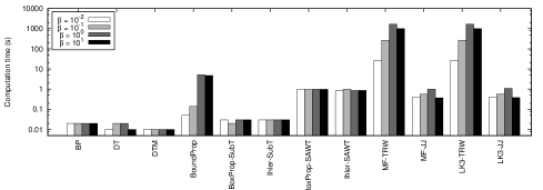
Figure 13: Results for grids with binary variables. The first four graphs show, for different values of the interaction strength $\beta$, the gaps of bounds on marginals calculated using different methods. Also shown for reference are the errors in the BP approximations to the same marginals. The final graph shows the total computation time for each method.

The results are shown in Figure 13. For very weak interactions ($\beta=10^{-2}$), BoxProp-SAWT gave the tightest bounds of all other methods, the only exception being BoundProp, which gave a somewhat tighter bound for 5 variables out of 25. For weak and moderate interactions ($\beta=10^{-1},1$), BoxProp-SAWT gave the tightest bound of all methods for each variable. For strong interactions ($\beta=10$), the results were mixed, the best methods being BoxProp-SAWT, BoundProp, MF-TRW and LK3-TRW. Of these, BoxProp-SAWT was the fastest method, whereas the methods using TRW were the slowest. For $\beta=10$, we present scatter plots in Figure 14 to compare the results of some methods in more detail. These plots illustrate that the tightness of bounds can vary widely over methods and variables.

Figure 14: Scatter plots comparing some methods in detail for grids with binary variables for strong interactions ($\beta=10$).

Among the methods yielding the tightest bounds, the computation time of our bounds is relatively low in general; only for low interaction strengths BoundProp is faster than BoxProp-SAWT. Furthermore, the computation time of our bounds does not depend on the interaction strength, in contrast with iterative methods such as BoundProp and MF-TRW, which need more iterations for increasing interaction strength (as the variables become more and more correlated). Further, as expected, BoxProp-SubT needs less computation time than BoxProp-SAWT but also yields less tight bounds. Another observation is that our bounds outperform the related versions of Ihler’s bounds.

4.2 Grids with ternary variables

To evaluate the bounds beyond the special case of binary variables, we have performed experiments on a $5\times 5$ grid with ternary variables and pairwise factors between nearest-neighbor variables on the grid. The entries of the factors were i.i.d., drawn by taking a random number from a normal distribution $\mathcal{N}\left(0,{\beta}^{2}\right)$ with mean $0$ and standard deviation $\beta$ and taking the $\exp$ of that random number.

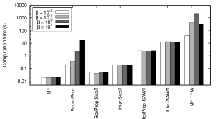
Figure 15: Results for grids with ternary variables. The first four graphs show, for different values of the interaction strength $\beta$, the gaps of bounds on marginals calculated using different methods. Also shown for reference are the errors in the BP approximations to the same marginals. The final graph shows the total computation time for each method.

The results are shown in Figure 15. We have not compared with bounds involving JJ or LK3 because these methods have only been formulated originally for the case of binary variables. This time, our method BoxProp-SAWT yielded the tightest bounds for all interaction strengths and for all variables (although this is not immediately clear from the plots).

4.3 Medical diagnosis

We also applied the bounds on simulated Promedas patient cases (Wemmenhove et al., 2007). These factor graphs have binary variables and singleton, pairwise and triple interactions (containing zeros). Two examples of such factor graphs are shown in Figure 16. Because of the triple interactions, less methods were available for comparison.

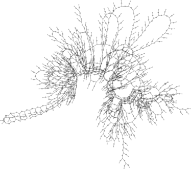
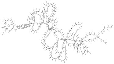
Figure 16: Two of the Promedas factor graphs.

The results of various bounds for nine different, randomly generated, instances are shown in Figure 17. The total number of variables for these nine instances was 1270. The total computation time needed for BoxProp-SubT was $51\,\mathrm{s}$, for BoxProp-SAWT $149\,\mathrm{s}$, for BoundProp more than $75000\,\mathrm{s}$ (we aborted the method for two instances because convergence was very slow, which explains the missing results in the plot) and to calculate the Belief Propagation errors took $254\,\mathrm{s}$. BoundProp gave the tightest bound for only 1 out of 1270 variables, BoxProp-SAWT for 5 out of 1270 variables and BoxProp-SubT gave the tightest bound for the other 1264 variables.

Figure 17: Results for nine different factor graphs corresponding to simulated Promedas patient cases. In reading order: Belief Propagation errors, BoundProp, BoxProp-SubT and BoxProp-SAWT.

Interestingly, whereas for pairwise interactions, BoxProp-SAWT gives tighter bounds than BoxProp-SubT, for the factor graphs considered here, the bounds calculated by BoxProp-SAWT were generally less tight than those calculated by BoxProp-SubT. This is presumably due to the local bound (5) needed on the SAW tree, which is quite loose compared with the local bound (2) that assumes independent incoming bounds.

Not only does BoxProp-SubT give the tightest bounds for almost all variables, it is also the fastest method. Finally, note that the tightness of these bounds still varies widely depending on the instance and on the variable of interest.

5 Conclusion and discussion

We have derived two related novel bounds on exact single-variable marginals. Both bounds also bound the approximate Belief Propagation marginals. The bounds are calculated by propagating convex sets of measures over a subtree of the computation tree, with update equations resembling those of BP. For variables with a limited number of possible values, the bounds can be computed efficiently. Empirically, our bounds often outperform the existing state-of-the-art in that case. Although we have only shown results for factor graphs for which exact inference was still tractable (in order to be able to calculate the BP error), we would like to stress here that it is not difficult to construct factor graphs for which exact inference is no longer tractable but the bounds can still be calculated efficiently. An example are large Ising grids (of size $m\times m$ with $m$ larger than 30). Indeed, for binary Ising grids, the computation time of the bounds (for all variables in the network) scales linearly in the number of variables, assuming that we truncate the subtrees and SAW trees to a fixed maximum size.

Whereas the results of different approximate inference methods usually cannot be combined in order to get a better estimate of marginal probabilities, for bounds one can combine different methods simply by taking the tightest bound or the intersection of the bounds. Thus it is generally a good thing to have different bounds with different properties (such as tightness and computation time).

An advantage of our methods BoxProp-SubT and BoxProp-SAWT over iterative methods like BoundProp and MF-TRW is that the computation time of the iterative methods is difficult to predict (since it depends on the number of iterations needed to converge which is generally not known a priori). In contrast, the computation time needed for our bounds BoxProp-SubT and BoxProp-SAWT only depends on the structure of the factor graph (and the chosen subtree) and is independent of the values of the interactions. Furthermore, by truncating the tree one can trade some tightness for computation time.

By far the slowest methods turned out to be those combining the upper bound TRW with a lower bound on the partition sum. The problem here is that TRW usually needs many iterations to converge, especially for stronger interactions where convergence rate can go down significantly. In order to prevent exceedingly long computations, we had to hand-tune the convergence criterion of TRW according to the case at hand.

BoundProp can compete in certain cases with the bounds derived here, but more often than not it turned out to be rather slow or did not yield very tight bounds. Although BoundProp also propagates bounding boxes over measures, it does this in a slightly different way which does not exploit independence as much as our bounds. On the other hand, it can propagate bounding boxes several times, refining the bounds more and more each iteration.

Regarding the related bounds BoxProp-SubT, BoxProp-SAWT and Ihler-SAWT we can draw the following conclusions. For pairwise interactions and variables that have not too many possible values, BoxProp-SAWT is the method of choice, yielding the tightest bounds without needing too much computation time. The bounds are more accurate than the bounds produced by Ihler-SAWT due to the more precise local bound that is used; the difference is largest for strong interactions. However, the computation time of this more precise local bound is exponential in the number of possible values of the variables, whereas the local bound used in Ihler-SAWT is only polynomial in the number of possible values of the variables. Therefore, if this number is large, BoxProp-SAWT may be no longer applicable in practice, whereas Ihler-SAWT still may be applicable. If factors are present that depend on more than two variables, it seems that BoxProp-SubT is the best method to obtain tight bounds, especially if the interactions are strong. Note that it is not immediately obvious how to extend Ihler-SAWT beyond pairwise interactions, so we could not compare with that method in that case.

This work also raises some new questions and opportunities for future work. First, the bounds can be used to generalize the improved conditions for convergence of Belief Propagation that were derived in (Mooij and Kappen, 2007) beyond the special case of binary variables with pairwise interactions. Second, it may be possible to combine the various ingredients in BoundProp, BoxProp-SubT and BoxProp-SAWT in novel ways in order to obtain even better bounds. Third, it is an interesting open question whether the bounds can be extended to continuous variables in some way. Finally, although our bounds are a step forward in quantifying the error of Belief Propagation, the actual error made by BP is often at least one order of magnitude lower than the tightness of these bounds. This is due to the fact that (loopy) BP cycles information through loops in the factor graph; this cycling apparently improves the results. The interesting and still unanswered question is why it makes sense to cycle information in this way and whether this error reduction effect can be quantified.

Acknowledgments

The research reported here is part of the Interactive Collaborative Information Systems (ICIS) project (supported by the Dutch Ministry of Economic Affairs, grant BSIK03024) and was also sponsored in part by the Dutch Technology Foundation (STW).

We thank Wim Wiegerinck for several fruitful discussions, Bastian Wemmenhove for providing the Promedas test cases, and Martijn Leisink for kindly providing his implementation of Bound Propagation.

References

• Cooper (1990) G.F. Cooper. The computational complexity of probabistic inferences. Artificial Intelligence, 42(2-3):393–405, March 1990.
• Georgii (1988) H.-O. Georgii. Gibbs Measures and Phase Transitions. Walter de Gruyter, Berlin, 1988.
• Ihler (2007) A. Ihler. Accuracy bounds for belief propagation. In Proceedings of the 23th Annual Conference on Uncertainty in Artificial Intelligence (UAI-07), July 2007.
• Jaakkola and Jordan (1996) T. S. Jaakkola and M. Jordan. Recursive algorithms for approximating probabilities in graphical models. In Proc. Conf. Neural Information Processing Systems (NIPS 9), pages 487–493, Denver, CO, 1996.
• Kschischang et al. (2001) F. R. Kschischang, B. J. Frey, and H.-A. Loeliger. Factor graphs and the sum-product algorithm. IEEE Trans. Inform. Theory, 47(2):498–519, February 2001.