Regular and Chaotic States in a Local Map Description of Sheared Nematic Liquid Crystals

Abstract

We propose and study a local map capable of describing the full variety of dynamical states, ranging from regular to chaotic, obtained when a nematic liquid crystal is subjected to a steady shear flow. The map is formulated in terms of a quaternion parametrization of rotations of the local frame described by the axes of the nematic director, subdirector and the joint normal to these, with two additional scalars describing the strength of ordering. Our model yields kayaking, wagging, tumbling, aligned and coexistence states, in agreement with previous formulations based on coupled ordinary differential equations. Such a map can serve as a building block for the construction of lattice models of the complex spatio-temporal states predicted for sheared nematics.

Driven complex fluids exhibit an unusual variety of dynamical statesDiat ; schmitt ; berret0 ; eiser ; sood ; sood1 ; salmon . When such fluids are sheared uniformly, the stress response is regular at very small shear rates. However, at larger shear rates the response is often intrinsically unsteady, exhibiting oscillations in space and time as a prelude to intermittency and chaossood ; sood1 ; Cladis . Such chaos associated with rheological response or “rheochaos”, occurs in regimes where the Reynolds number is very small. It must thus be a consequence of constitutive and not convective non-linearities, originating in the coupling of the flow to structural or orientational variables describing the local state of the fluidCates_Fielding ; Olmsted_Faraday . The diverse possibilities for internal degrees of freedom in complex fluids, such as the orientation of nematogenic molecules, layer stacking in lamellar and onion phases and heterogeneities arising from local jamming in colloidal suspensions, implies that the study of the rheology of complex fluids should illuminate a variety of non-trivial steady states in driven soft matter.

Recent rheological studies of “living polymers”, solutions of worm-like micelles in which the energies for scission and recombination are thermally accessible, obtain an oscillatory response to steady shear at low shear rates which turns chaotic at larger shear ratessood ; sood1 . It has been argued that a hydrodynamic description of this behaviour requires a field describing the local orientation of the polymer, motivating a treatment of the problem of an orientable fluid, such as a nematic, in a uniform shear flowhess30 ; doi ; MD . Nonlinear relaxation equations for the symmetric, traceless second rank tensor ${\bf Q}$ characterizing local order in a sheared nematic have been derived hess30 ; doi ; MD ; hess36 ; hess20 ; MD1 ; Olmsted ; HS . Assuming spatial uniformity, a system of 5 coupled ordinary differential equations (ODEs) for the 5 independent components of ${\bf Q}$ in a suitable tensor basis is obtained. Solving this system of equations yields a complex phase diagram admitting many states – aligned, tumbling, wagging, kayak-wagging, kayak-tumbling and chaotic – as functions of the shear rate $\dot{\gamma}$ and a phenomenological relaxation time which is a parameter in the equations of motionGR1 ; GR2 ; Grosso . Recent work adds spatial variations: numerical studies of the partial differential equations thus obtained yield a phase diagram containing spatio-temporally regular, intermittent and chaotic statessr ; sr1 .

The degrees of freedom which enter a coarse-grained description of an orientable fluid are mesoscopic. Spatio-temporal structure arises from the coupling of locally ordered regions, through processes such as molecular diffusion, flow-induced dissipation and advection. A powerful approach to understanding complex spatio-temporal dynamics is based on the study of coupled map lattices, a numerical scheme in which maps placed on the sites of a lattice evolve both via local dynamics as well as through couplings to neighbouring siteskaneko . However, the utility of this methodology in a specific context is often severely limited by the availability of local maps able to describe the spatially uniform case. This paper addresses this requirement in the context of a model for rheochaos, proposing the first local map description of the regular and chaotic states obtained in sheared nematics.

There is, in general, no systematic procedure for the construction of such maps. However, it is reasonable to require that any such map should accurately reproduce the full variety of states obtained through the study of the corresponding ODEs. It should also enable useful physical insights through a sensible choice of physical variables. One obvious possibility is simply the discretization of the governing ODEs. Such a choice of variables, however, is not particularly illuminating as these equations are formulated in terms of the components of ${\bf Q}$ in a specific space-fixed tensor basis, rather than in terms of variables more natural to the problem.

We have thus explored an alternative formulation of this problem, constructing a local map in terms of quaternion variables. These variables encode the dynamics of the orthogonal set of axes associated with the eigenvectors of ${\bf Q}$, i.e. the director, sub-director and the joint normal to these. Our approach incorporates biaxiality, is formulated in terms of physically accessible variables and is computationally straightforward to implement. Our results, summarized in the phase diagram of Fig. 1, are in good agreement with previous work based on ODEs GR2 , but provide an efficient alternative to such methodsfootnote2 .

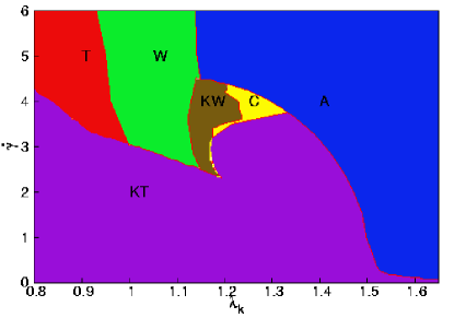
Figure 1: [Color online] The phase diagram of steady states in our model, illustrating regimes in which the following steady states are obtained for a generic initial condition: an aligned state denoted as ‘A’, a tumbling state labelled as ‘T’, a wagging state ‘W’, a kayak-tumbling state ‘KT’, a kayak-wagging state denoted by ‘KW’ and a complex state denoted as ‘C’. This phase diagram closely resembles phase diagrams plotted in Refs. GR2 .

Defining $\widehat{\bf b}:=\frac{1}{2}({\bf b}+{\bf b}^{T})-\frac{1}{3}(tr{\bf b}){\bf\delta}$ to be the symmetric-traceless part of the second-rank tensor b, the equation of motion for ${\bf Q}$ in a passive velocity field is hess30 ; GR2 :

$$\frac{d{\bf Q}}{dt}-2\widehat{{\bf\Omega\cdot Q}}-2\sigma\widehat{{\bf\Gamma\cdot Q}}+\tau_{Q}^{-1}{\bf\Phi}=-\sqrt{2}\frac{\tau_{ap}}{\tau_{a}}{\bf\Gamma}$$ (1)

where the tensor ${\bf\Omega}=\frac{1}{2}((\nabla{\bf v})^{T}-\nabla{\bf v})$, ${\bf\Gamma}=\frac{1}{2}((\nabla{\bf v})^{T}+\nabla{\bf v})$ and $\nabla{\bf v}$ is the velocity gradient tensor, with ${\bf v}=\dot{\gamma}y{\bf e^{x}}$, where ${\bf e^{x}}$ is a unit vector in the $x-$ direction. The velocity is along the $x$ direction, the velocity gradient is along the $y$ direction, while $z$ is the vorticity direction. The quantities $\tau_{a}>0$ and $\tau_{ap}$ are phenomenological quantities related to relaxation times, $\sigma$ describes the change of alignment caused by ${\bf\Gamma}$ and ${\bf\Phi}=\partial\phi/\partial{\bf Q}$, with $\phi({\bf Q})=\frac{1}{2}A{\bf Q:Q}-\frac{1}{3}\sqrt{6}B({\bf Q\cdot Q}):{\bf Q}+\frac{1}{4}C({\bf Q:Q})^{2}$. The notation $Q:Q$ represents $Q_{ij}Q_{ji}$, with repeated indices summed over. Here $A=A_{0}(1-T^{*}/T)$, and $B$ and $C$ are constrained by the conditions $A_{0}>0$, $B>0,C>0$ and $B^{2}>\frac{9}{2}A_{0}C$. Scaling $t=t^{*}\tau_{a}/A_{k}$, ${\bf v}={\bf v^{*}}A_{k}/\tau_{a}$ and $a=a^{*}a_{k}$, Eqn. (1) can be written in dimensionless form, $\frac{d{\bf Q^{*}}}{dt^{*}}-2\widehat{{\bf\Omega^{*}.Q^{*}}}-2\sigma\widehat{{\bf\Gamma^{*}.Q^{*}}}+(\theta{\bf Q}^{*}-3\sqrt{6}\widehat{{\bf Q^{*}.Q^{*}}}+2({\bf Q^{*}:Q^{*})Q^{*}})=\sqrt{\frac{3}{2}}\lambda_{k}{\bf\Gamma^{*}}$ where $A_{k}=A_{0}(1-T^{*}/T_{k})=2B^{2}/9C,a_{k}=a_{eq}(T_{k})=2B/3C$ is the (nonzero) equilibrium value of the scalar order parameter $a$ at the transition temperature $T_{k}$,  $\lambda_{k}=-\frac{2}{3}\sqrt{3}\frac{\tau_{ap}}{\tau_{a}a_{k}}$ and $\theta=(1-\frac{T^{*}}{T})/(1-\frac{T^{*}}{T_{k}})$ is the reduced temperature.

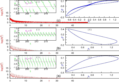
Figure 2: [Color Online] The sequence of three main panels shows the power spectrum associated with states in the regimes labelled (a) T and (b) W in the phase diagram of Fig. 1. The topmost panel (c) shows a mixed state (M) (not shown separately in Fig. 1), associated with the boundary between W and T The inset labelled (i) in all these panels shows typical plots of the time-dependence of the z-component of the director $n_{z}$ and the angle $\phi$ made by the projection of the director on the $x-y$ plane with the $x-$ axis. The insets labelled (ii) in all these panels show the trajectory in the $s_{1}-s_{2}$ plane.

The ${\bf Q}$ tensor admits the following parametrization: $Q_{ij}=\frac{3s_{1}}{2}\left(n_{i}n_{j}-\frac{1}{3}\delta_{ij}\right)+\frac{s_{2}}{2}\left(m_{i}m_{j}-l_{i}l_{j}\right)$, where $s_{1}$ and $s_{2}$ represent the magnitude of the ordering along n (the director) and m (the subdirector), with n and m unit vectors and l = n $\times$ m. The dynamics of ${\bf Q}$ thus involves both the dynamics of the frame defined by ${\bf n},{\bf m}$ and ${\bf l}$ as well as the dynamics of $s_{1}$ and $s_{2}$. The frame dynamics can be represented in many equivalent ways, such as through coordinate matrices, axis-angle or Euler angle representations. However, the coordinate matrix representation requires a large number of parameters, the axis-angle representation suffers from redundancy and the use of the Euler-angle representation is marred by the “gimbal-lock” problemgimbal-lock . Our parametrization of the frame dynamics uses quaternion variables, providing an elegant, compact and numerically stable alternative to these representations.

Equations for $\dot{\bf{n}}$, $\dot{\bf{m}}$ and $\dot{\bf{l}}$ as well as for the order parameter amplitudes $\dot{s_{1}}$ and $\dot{s_{2}}$ can be derived by considering a reference frame in which the director and subdirector are stationary (body frame). In the body frame, denoted by primed vectors, the director can be chosen to be ${\bf n}^{\prime}=(1,0,0)$, the subdirector to be ${\bf m}^{\prime}=(0,1,0)$, with ${\bf l}^{\prime}=(0,0,1)$. The transformation matrix ${\bf A}$ which maps vectors from the lab frame to the body frame, can be defined in terms of quaternion parameters $(e_{0},\ldots,e_{4})$ constrained by $e_{0}^{2}+e_{1}^{2}+e_{2}^{2}+e_{3}^{2}=1$amatrix . The quantities ${\bf n}=(n_{x},n_{y},n_{z}),{\bf m}=(m_{x},m_{y},m_{z})$ and ${\bf l}=(l_{x},l_{y},l_{z})$ are easily obtained using this mapping, yielding ODE’s for the parameters ${s_{1},s_{2},e_{0},e_{1},e_{2},e_{3},e_{4}}$. These are converted into a map using a first-order Euler scheme. After each discrete time step, we renormalise the quaternion variable. Choosing $\sigma$ and $\theta$ equal to zero for all the results reported here in common with earlier work, our map is then defined through

$${s_{1}}^{t+1} ={s_{1}}^{t}+ \Delta\left(\frac{1}{6}\ \{9\ \sqrt{6}\ s_{1}^{2}-18\ s_{1}^{3}-3\ \sqrt{6}\ s_{2}^{2}-6\ s_{1}\ s_{2}^{2}+3\ \sqrt{6}\ n_{x}\ n_{y}\ \dot{\gamma}\ \lambda_{k}\}\right)^{t}$$

$${s_{2}}^{t+1} ={s_{2}}^{t}+ \Delta\left(-3\ \sqrt{6}\ s_{1}\ s_{2}-3\ s_{1}^{2}\ s_{2}-s_{2}^{3}-\sqrt{\frac{3}{2}}\ (l_{x}\ l_{y}-m_{x}\ m_{y})\ \dot{\gamma}\ \lambda_{k}\right)^{t}$$

$${e_{0}}^{t+1} ={e_{0}}^{t}+ \Delta\Bigg{(}\frac{1}{4}\dot{\gamma}\ e_{3}+\frac{1}{4}\ \sqrt{\frac{3}{2}}\ \dot{\gamma}\ \{-\frac{(l_{y}\ m_{x}+l_{x}\ m_{y})\ e_{1}}{s_{2}}+\frac{2\ (l_{y}\ n_{x}+l_{x}\ n_{y})\ e_{2}}{3\ s_{1}+s_{2}}$$

$$+\frac{2\ (m_{y}\ n_{x}+m_{x}\ n_{y})\ e_{3}}{-3\ s_{1}+\ s_{2}}\}\ \lambda_{k}\Bigg{)}^{t}$$

$${e_{1}}^{t+1} ={e_{1}}^{t}+ \Delta\Bigg{(}\frac{1}{4}\ \dot{\gamma}\ e_{2}\ +\frac{1}{4}\ \sqrt{\frac{3}{2}}\ \dot{\gamma}\ (\frac{(l_{y}\ m_{x}+l_{x}\ m_{y})\ e_{0}}{s_{2}}-\frac{2\ \ (m_{y}\ n_{x}+m_{x}\ n_{y})\ e_{2}}{-3\ s_{1}+s_{2}}$$

$$+\frac{2\ (l_{y}\ n_{x}+l_{x}\ n_{y})\ \ e_{3}}{3\ s_{1}+s_{2}})\ \lambda_{k}\Bigg{)}^{t}$$

$${e_{2}}^{t+1} =e_{2}^{t}+ \Delta\Bigg{(}-\frac{1}{4}\ \dot{\gamma}\ e_{1}\ +\frac{1}{4}\ \sqrt{\frac{3}{2}}\ \dot{\gamma}\ (-\frac{2\ (l_{y}\ n_{x}+l_{x}\ n_{y})\ e_{0}}{3\ s_{1}+s_{2}}+\frac{2\ (m_{y}\ n_{x}+m_{x}\ n_{y})\ e_{1}}{-3\ s_{1}\ +s_{2}}$$

$$+\frac{(l_{y}\ m_{x}+l_{x}\ m_{y})\ e_{3}}{s_{2}})\ \lambda_{k}\Bigg{)}^{t}$$

$${e_{3}}^{t+1} =e_{3}^{t}+ \Delta\Bigg{(}-\frac{1}{4}\ \dot{\gamma}\ e_{0}\ +\frac{1}{4}\ \sqrt{\frac{3}{2}}\ \dot{\gamma}\ (-\frac{2\ (m_{y}\ n_{x}+m_{x}\ n_{y})\ e_{0}}{-3\ s_{1}+s_{2}}-\frac{2\ (l_{y}\ n_{x}+l_{x}\ n_{y})\ e_{1}}{3\ s_{1}+s_{2}}\$$ (2)

$$-\frac{(l_{y}\ m_{x}+l_{x}\ m_{y})\ e_{2}}{s_{2}})\ \lambda_{k}\Bigg{)}^{t}$$

We choose $\Delta=0.01$ for all our calculations. (The phase boundaries shown in Fig. 1 exhibit a weak dependence on $\Delta t$. However, provided $\Delta t$ is chosen small enough, this dependence may be neglected.) The superscript ‘t’ indicates that the values of the variables are taken at the t’th discrete time step. The control parameters are the dimensionless shear rate $\dot{\gamma}$ and $\lambda_{k}$. In place of the 5 coupled ODE’s used in the conventional parametrization of the dynamics of ${\bf Q}$, we have 6 equations constrained by the normalization requirement, thereby conserving the number of degrees of freedom.

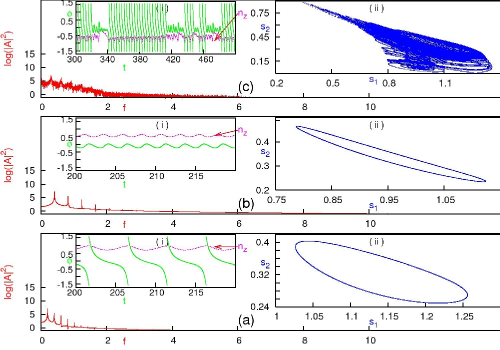
Figure 3: [Color online] The sequence of three main panels shows the power spectrum associated with states in the regimes labelled (a) KT (kayak-tumbling), (b) KW (kayak-wagging) and (c) C (complex or chaotic) in the phase diagram of Fig. 1. The inset labelled (i) in all these panels shows typical plots of the time-dependence of the z-component of the director $n_{z}$ and the angle $\phi$ made by the projection of the director on the $x-y$ plane with the $x-$ axis. The insets labelled (ii) in all these panels show the trajectory in the $s_{1}-s_{2}$ plane.

In our numerical analysis of the map, we start typically from random initial conditions, omitting sufficient transients ($\sim 10^{5}$ time steps) to ensure that the asymptotic attractor of the dynamics is reached. Our analysis includes inspection of the (i) power spectrum, (ii) phase portraits, (iii) bifurcation diagrams and (iv) time series of the different relevant variables. Figs.  2 and  3 show the variety of states obtained in our numerical calculations. Each sub-figure, labelled as Figs. 2 (a) - (c) and Figs.  3 (a)-(c), has the following structure: The first inset, labelled (i) for all figures, describes the time dependence of $n_{z}$, the z-component of the director, and the angle $\phi$ made by the projection of the director on the $x-y$ plane with the $x-$ axis. The second inset, labelled (ii) for all figures, plots the quantities measuring the amount of ordering along director and sub-director against each other, providing the attractor of the system in the $s_{1}-s_{2}$ plane for a generic initial condition. The main panel in each of the sub-figures shows the power spectrum of $s_{1}$, $\ln(|A(f)|^{2})$ against frequency $f$ on a semi-log plot.

The following states are easily identified: (I) An Aligned state denoted as ‘A’ in the phase-diagram of Fig. 1, but omitted, for brevity, from the states shown in Fig. 2 and Fig. 3. In the aligned state, neither the frame orientation, nor $s_{1}$ and $s_{2}$, vary in time. The director is aligned with the flow at a fixed angle; (II) A Tumbling state, in which the director lies in the shear plane (the $xy$ plane) and rotates about the vorticity direction (the $z$ axis). Fig. 2(a)(i) indicates that this state is a stable in-plane state, since the z-component of the director is zero. Also, the angle made by the projection of the director on the x-y plane varies smoothly between $\pi/2$ and -$\pi/2$. Fig. 2(a)(ii) shows the periodic character of this state. This state is labelled as ‘T’ in the phase-diagram of Fig.1; (III) A Wagging state, in which the director lies in the shear plane, but oscillates between two values. Note that Fig.  2 (b)(i) indicates that this state is a stable in-plane state. Also, the director oscillates back and forth in-plane as indicated in Fig.  2 (b)(ii). Fig.  2 (b) shows that this state is a periodic state with sharp delta-function peaks in the power spectrum. These states are denoted as ‘W’ in the phase-diagram in Fig.1. In addition, we obtain (IV) A Kayak-Tumbling state, equivalent to the tumbling state, but in which the director is out of the shear plane. Thus, as shown in Fig. 3(a) $n_{z}\neq 0$ and the projection of the director on the $xy$ plane rotates through a full cycle. Such states are temporally periodic, as shown in Fig. 3(a); the regular cycles evident in the map of $s_{1}$ vs. $s_{2}$ (Fig. 3(a)(ii)) is a further indication of periodic behaviour. These states are noted as ‘KT’ in the phase-diagram of Fig.  1; (V) A Kayak-Wagging state where, as in KT, the director is out of plane, but the projection of the director on the shear plane oscillates between two values. The properties of such states are illustrated in Fig. 3(b). Such states are again temporally periodic. The cyclic trajectory of the system in the $s_{1}-s_{2}$ plane (Fig. 3(b)(ii)) further confirms such periodic behaviour. These states are denoted by ‘KW’ in the phase-diagram of Fig. 1; (VI) A Mixed state, typically found close to the boundaries between wagging and tumbling states, whose properties are illustrated in Fig. 2(c). In such states, the director exhibits both oscillation and complete rotations. Power spectra obtained at the boundaries of this phase, for example near $\lambda_{k}=0.99$ and $\dot{\gamma}=4.0$, have a broad range of frequencies, and, (VII) A Complex state, in which the director lies out of the shear plane but both oscillates and rotates. The complex phase exhibits chaotic behaviour, as can be seen in Fig. 3(c). Note that the delta function peaks in the power spectrum exhibited by the periodic states discussed earlier have broadened into a continuum of frequencies. The plot of $s_{1}$ vs. $s_{2}$ displays no regular structure. These state are noted as ‘C’ in the phase-diagram in Fig.1. In addition to these states, we also obtain a log rolling state in which the director is perpendicular to the shear plane (not shown).

The range of dynamical states manifest in this problem is also evident from bifurcation diagrams obtained at fixed $\dot{\gamma}=4.0$, varying $\lambda_{k}$. Such a cut intersects KT, T, W, KW, C and A states in the phase diagram. The quantities $n_{z}$ and the Poincare section of $s_{1}$ show that $n_{z}=0$ for the T, W and A states, while the KT, KW and C states are out-of-plane states with $n_{z}\neq 0$. Further, the $s_{1}$ section, displays a fixed point for the aligned state, regular cycles for the KT, T W and KW states and irregular (chaotic) behavior for the C state.

Aradian and Cates have recently studied a minimal model for rheochaos in shear-thickening fluids, using equations which describe a shear-banding system coupled to a retarded stress responsearadian_cates . These authors connect their model system to a modified Fitzhugh-Nagumo model, a dynamical system with a variety of interesting and complex phases. Fielding and Olmsted study instabilities in shear-thinning fluids, where the instability originates in the multi-branched character of the constitutive relationfielding_olmsted . Chakrabarty et al. report a study of the PDE’s describing the dynamics of ${\bf Q}$, characterizing spatio-temporal routes to chaotic behaviour in sheared nematics sr . These studies allow for spatial variation - although restricted so far to the one-dimensional case - whereas our local map describes the spatially uniform situation. However, the dynamical system we study is obtained directly from the underlying dynamics, in contrast to the approaches of Refs. aradian_cates ; fielding_olmsted . Whether coupling maps of the sort we construct permits a complete description of the spatio-temporal structure obtained in Ref. sr remains to be seen.

In conclusion, we have proposed a local map describing the variety of dynamical states obtained in a model for sheared nematics. Our phase diagram, Fig. 1, contains all non-trivial dynamical states obtained in previous work. It also closely resembles, even quantitatively, phase diagrams obtained in previous work which used ordinary differential equations formulated in continuous time. Our work thus supplies a crucial ingredient in the construction of coupled map lattice approaches to the spatio-temporal aspects of rheological chaos, a problem currently at the boundaries of our understanding of the dynamics of complex fluids.