Type I and type II neuron models are selectively driven by differential stimulus features

Abstract

Neurons in the nervous system exhibit an outstanding variety of morphological and physiological properties. However, close to threshold, this remarkable richness may be grouped succinctly into two basic types of excitability, often referred to as type I and type II. The dynamical traits of these two neuron types have been extensively characterized. It would be interesting, however, to understand the information-processing consequences of their dynamical properties. To that end, here we determine the differences between the stimulus features inducing firing in type I and in type II neurons. We work both with realistic conductance-based models and minimal normal forms. We conclude that type I neurons fire in response to scale-free depolarizing stimuli. Type II neurons, instead, are most efficiently driven by input stimuli containing both depolarizing and hyperpolarizing phases, with significant power in the frequency band corresponding to the intrinsic frequencies of the cell.

1 Introduction

Several research lines have recently used reverse correlation methods to determine the stimulus features that are most relevant in shaping the probability to generate spikes of sensory neurons. Just to mention a few examples, in the visual system, Fairhall, Burlingame, Narasimhan, Harris, Puchalla and Berry (2006) revealed multiple spatio-temporal receptive fields (STRF) driving salamander retinal ganglion cells. In turn, Rust, Schwartz, Movshon, and Simoncelli (2005) explored the STRF of macaque V1. In the somatosensory system, Maravall, Petersen, Fairhall, Arabzadeh, and Diamond (2007) employed covariance analysis to disclose the effect of adaptation on the shift of coding properties in rat barrel cortex.

Here, we are interested in exploring the way the relevant stimulus features driving neuronal firing depend on the intrinsic dynamical properties of the cell. To that end, we work with a time-dependent stimulus representing the total input current arriving at the axon hillock. In any real system, this input current may enter into the cell in several ways. For example, it can pass through receptor channels, activated by specific physical agents (light, sound, temperature, etc.) relevant to a particular sensory modality. Alternatively, it may be the integrated synaptic current entering a central cell through its numerous dendrites, or through an intracellular electrode. In any case, we shall assume that our time-dependent stimulus $s(t)$ represents a ionic current that, after propagating all along the spatial extension of the neuron, arrives into the axon hillock, where the decision to fire or not to fire is taken. Hence, we shall only be dealing with the temporal - and not spatial - properties of the input current.

Our aim is to understand the relation between the stimulus attributes that most strongly affect the firing probability and the intrinsic dynamical properties of the neurons. This line of research was initiated with the study of the relevant stimulus features driving integrate-and-fire model neurons (Agüera y Arcas & Fairhall, 2003) and in Hodgkin-Huxley cells (Agüera y Arcas, Fairhall, & Bialek 2003). Later on, Hong, Agüera y Arcas and Fairhall (2007) explored a broader class of neuron models, determining the effect of several dynamical features on the relevant stimulus dimensions. Here, we extend those analysis, searching for unifying properties that characterize the way in which the type of bifurcation at firing onset affects stimulus selectivity and information transmission. We therefore compare the relevant stimulus features driving two broad classes of neuron models, namely, type I and type II dynamics. The distinction between type I and type II excitability was first introduced by Hodgkin (1948), when studying the dependence of the firing rate of a neuron with the injected current. Later, more detailed classifications of neuronal excitability were introduced (Ermentrout 1996, Izhikevich 2007), in terms of the bifurcation type at firing onset. In all cases, type I cells undergo a saddle-node bifurcation on the invariant circle, at threshold. Type II neurons, instead, may correspond to 3 different bifurcations, namely, a subcritical Hopf bifurcation, a supercritical Hopf bifurcation, or a saddle node bifurcation outside the invariant circle. Most of type II conductance-based Hodgkin-Huxley type neuron models, however, undergo a subcritical Hopf bifurcation. Therefore, here, when exploring type II neuron models, we shall focus on those exhibiting a subcritical-Hopf bifurcation.

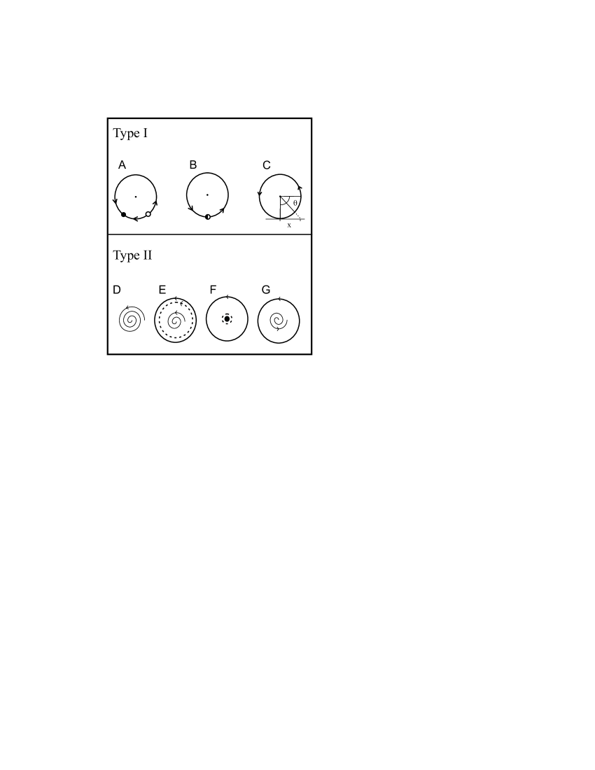
Figure 1: Schematic representation of the bifurcation underlying the onset of firing in type I (A, B, C) and type II (D, E, F, G) neuronal models. The input current is increased from left to right, and in both cases, the system passes from a single fixed point (A and D) describing the subthreshold rest state, to a firing limit cycle (C and G).

When type I neurons are stimulated by a constant input current, the onset of firing is brought about by a saddle node bifurcation (Izhikevich, 2007). In the upper panel of Fig. 1, a schematic representation of the topology of a type I bifurcations is depicted. For subthreshold input currents (A), the system contains two orbits forming a closed figure, connecting two fixed points: one of them is stable, and the other is unstable. As the injected current $I$ increases, the two fixed points come nearer to each other, so that when $I$ reaches a critical value $I_{\rm c}$, the two points coalesce into a single one (B). Thereafter, both equilibrium points disappear, and the system moves in a periodic orbit (C).

The topological properties of the subcritical Hopf bifurcation (also called inverted Hopf bifurcation) characteristic of many type II models are shown in the lower panel of Fig. 1. For subthreshold input currents, there is only a single stable spiral fixed point (D). As the current increases, there is a region far away from the fixed point where the radial velocity diminishes. At a certain critical current $I_{\rm g}$, two closed orbits appear through a global bifurcation, the outermost stable, the inner one unstable (E). As the current is increased further, the unstable limit cycle shrinks, approaching the spiral fixed point (F). When $I$ reaches a second critical value $I_{\rm c}$, the unstable orbit coalesces onto the fixed point. If $I$ grows beyond $I_{\rm c}$, the fixed point is turned into an unstable spiral node, and the only stable attractor of the system is the distant limit cycle (G).

These two types of cells differ from each other in the bifurcation underlying the onset of firing. This comprises a clear topological difference, that endows each type with specific dynamical properties. It would be interesting, however, to be able to identify the functional consequences of these dynamical differences. More precisely, we would like to determine in which way the two neuron types differ, regarding their information-processing properties. Specifically, what kind of time-dependent stimulus is needed to induce spiking in a type I neuron, and how does this stimulus differ from the one needed to excite a type II neuron? To answer this question, we explore the relevant stimulus features shaping the firing probability of type I and type II neurons, by means of covariance analysis. In the first place, we work with conductance-based models, capturing the biophysically relevant processes. We then compare the results obtained for these realistic models with those derived from reduced neural models, which minimally describe the essential dynamical features of both neuronal types. We conclude that close to threshold, the relevant stimulus features driving a given cell are determined by the type of bifurcation.

2 The models and their phase-resetting curves

In the case of type I neurons, we use the model neurons introduced by Wang and Buzsaki (1996) to describe hippocampal interneurons. This model (hereafter called “WB”) when stimulated with a supra-threshold constant input current settles into a limit cycle, embedded in its 3-dimensional phase space. As the input current is lowered, the firing frequency tends to zero, and the system displays a saddle-node bifurcation into its resting state. Therefore, the WB model can be classified as type I. The detailed equations are displayed in Appendix A. The second model is the original Hodgkin-Huxley (HH) neuron (see the equations in Appendix B). This is a 4-dimensional system which, at threshold, undergoes a subcritical Hopf bifurcation, and is therefore classified as type II.

Figure  1 shows the qualitative behavior of type I and type II neural models upon constant stimulation. We see that both systems oscillate periodically if the input is above the critical current $I_{\rm c}$. The behavior of these systems when weakly perturbed by rapid current injections is characterized by the phase-response function $Z(t)$. This function describes how the phase of a spike is advanced or delayed, depending on the time $t$ at which the system is perturbed (Kuramoto, 2003). More precisely, $Z(t)$ is defined as the ratio between the change of the phase and the size of the perturbation in the limit of small perturbations. In principle the perturbation can be applied along any of the variables of the dynamical system, giving rise to a multi-dimensional phase-response function. In this paper, however, perturbations are only instantiated as input currents, thereby only affecting a single direction in phase space: the one parallel to the membrane potential axis $V$. Hence, here, $Z(t)$ represents the magnitude of a phase-response function always pointing in the direction of $V$ (or $-V$, if $Z(t)$ is negative). By convention, we stipulate that the time of spike generation (defined as the point where the voltage crosses the value 0 mV from below) corresponds to $t=0$. The function $Z(t)$ has the same period $T$ as the firing cycle of the neuron which, in turn, depends on the size of the constant input current.

In panels A and B of Fig. 2 the phase-response curve of the WB and HH models is depicted. The most salient difference between the two models is that $Z(t)$ is (almost) always positive for the WB model, whereas it exhibits both positive and negative regions in the HH case (Hansel, Mato & Meunier, 1995). Hence, a small depolarizing perturbation always results in anticipated firing in the WB model, whereas it may either advance or delay spiking in the HH model, depending on when exactly the perturbation is delivered. Both the WB and HH models show maximal sensitivity to the external perturbation far away from the spiking events. In addition, the HH model shows more evidently that right after the spike ($t\approx 0$), the system is rather unresponsive to incoming perturbations, due to refractoriness.

Figure 2: Type I (left panels) and type II (right panels) phase response curves. The realistic models (WB and HH) are shown in the upper row, and the simplified normal forms are depicted in the bottom row.

In the upper panels of Fig. 2, the DC component of the input current was fixed to a different value in each model, so as to obtain a firing rate of 62.5 Hz in both cases (that is, $T=16$ ms). When the DC input current is lowered, the HH model eventually enters in its bistable region at a finite firing frequency. The WB model, instead, can be driven with arbitrarily low firing rates. Actually, as the firing rate of the WB model is diminished, the small region of negative $Z(t)$ that is observed for $t\approx T$ and $t\approx 0$ disappears, leaving a purely positive phase-resetting curve. In fact, only near threshold do type I neurons display a purely positive phase-resetting; if the input current increases, the curve begins to resemble that of type II neurons.

Near threshold, hence, the HH neuron shows a phase-resetting curve that is qualitatively different from that of the WB neuron. The question now arises whether this difference is specific to these two neuron models, or whether it is always found when comparing a type I with a type II cell. We therefore analyze the phase-resetting curves of the reduced models. To that end, the input current is written as

$$I=I_{\rm c}+\epsilon^{2}i.$$ (1)

Ermentrout & Kopell (1986) and Ermentrout (1996) have shown that the dynamics of any type I neuron can be reduced to a 1-dimensional equation for a variable $x$ that represents the projection of the state of the system on the direction of phase space that loses stability at threshold. After a non-linear transformation $x=\tan(\theta/2)$, and rescaling the temporal variable this dynamics can be written as

$$\frac{{\rm d}\theta}{{\rm d}t}=\left[1-\cos(\theta)\right]+\alpha\left[1+\cos\theta\right],$$ (2)

where $\alpha=\eta/2\epsilon q$ plays the role of a bifurcation parameter. It is defined in terms of $q$ (depending solely on the dynamical properties of the original model) and $\eta$ (proportional to the magnitude of the perturbation $i$). Both parameters may be derived from the equations of the full-blown system. Spike generation is associated to $\theta=\pm\pi$ (see Fig. 1). Notice that Eq. (2) is valid for any neural model sufficiently close to a saddle-node bifurcation. Hence, irrespective of the diversity of dynamical richness, near firing onset the whole collection of type I conductance-based models is topologically equivalent to a system controlled by just a single parameter $\alpha$.

For 1-dimensional systems, the phase response curve can be evaluated analytically (Hansel, Mato & Meunier, 1995; Kuramoto, 2003). For this case it is found that

$$Z(t)\propto\sin^{2}\left(\pi t/T\right),$$ (3)

as depicted in Fig. 2C. Notice that, as in the WB model, $Z(t)$ is always positive, with maximum sensitivity near $t=T/2$. Therefore, up to some positive scaling constant, the response function of type I models near the bifurcation is universal. In what follows, all numerical integrations of the reduced (or normal) type I system are carried out with Eq. (2).

Why is the phase response function always positive for type I neurons, and why does it approach zero in the vicinity of spiking times? Near the bifurcation, type I neurons spend most of their time in the neighborhood of $\theta=0$ or $x=0$ (that is, far away from the spiking region $\theta=\pi$ or $x\to\pm\infty$). The slow dynamics near $\theta=0$ is a footprint of the two fixed points that appear through a saddle-node bifurcation, when the input current is lowered below the critical value. As a consequence, in the slightly supra-threshold regime, the system spends a large fraction of each period around $x=0=\theta$. Hence, almost all the perturbations find the system in this region, where positive perturbations advance the phase of the neuron. Therefore, for almost all $t$, external perturbations result in anticipated spike generation and thereby, in a positive phase-response curve. In addition, in the vicinity of $\theta=\pm\pi$, the system sets into the rapid acceleration associated with spike generation. In this region, the dynamics is dominated by the catalytic opening of voltage-dependent conductances, and not by the detailed temporal properties of the perturbing current. Hence, $Z(t)\to 0$, when $t\approx T$.

We now turn to the reduced model of the HH neuron. In this case, the onset of firing is governed by a subcritical Hopf bifurcation. Only two of the four eigenvalues lose stability at threshold, meaning that the bifurcation takes place in two dimensions. Hence, the reduced model is 2-dimensional, and similarly to Brown et al. (2004), we choose to analyze it in polar coordinates

$$\frac{{\rm d}r}{{\rm d}t} = \alpha r+cr^{3}+fr^{5}$$ (4)

$$\frac{{\rm d}\phi}{{\rm d}t} = 2\pi(\beta+dr^{2}+gr^{4})$$ (5)

where, for subcritical bifurcations, $c>0$ , $f<0$. Notice that the reduced system described by Eqs. (4) and (5) represents a combination of two bifurcations: a non-local saddle-node bifurcation of limit cycles far away from the fixed point (represented in Fig. 1E), and a local subcritical Hopf bifurcation (Fig. 1F). This means that the parameters defining the spatially extended system (4) and (5) cannot be obtained by a local reduction of the full-blown model. Therefore, they have to be understood as an approximate representation of the original system, with its same topological properties.

The bifurcation parameter $\alpha$ is proportional to $I-I_{\rm c}$. When $\alpha>0$ the fixed point $r=0$ is unstable, and all trajectories tend to a limit cycle located at $r=[-c(1+\sqrt{1-4\alpha f/c^{2}})/2f]^{1/2}$, corresponding to the regular firing trajectory. If $\alpha$ is decreased such that $c^{2}/4f<\alpha<0$, then $r=0$ becomes a stable fixed point, and it coexists with a stable limit cycle at $r=[-c(1+\sqrt{1-4\alpha f/c^{2}})/2f]^{1/2}$. The two attractors are separated by an unstable limit cycle located at $r=[-c(1-\sqrt{1-4\alpha f})/2c^{2}]^{1/2}$. If $\alpha$ is decreased even further, such that $\alpha<c^{2}/4f$, a single stable manifold remains: a fixed point at $r=0$, representing the subthreshold resting state.

The stable limit cycle of the firing trajectory has a minimal radius of $\sqrt{-c/2f}$, when $\alpha=c^{2}/4f$. Therefore, spike generation will be associated to the moment where the system crosses the border $\theta=\pi$ with a radius $r\geq\sqrt{-c/2f}$.

As before, the phase resetting curves can be evaluated analytically (Brown, Moehlis, & Holmes, 2004)

$$Z(t)\propto\sin\left[2\pi(t-t_{0})/T\right],$$ (6)

where $t_{0}$ and the proportionality constant can be evaluated in terms of the parameters of the original HH model. Fig. 2D depicts the phase response curve of Eq. (6). As observed in the full HH model, external perturbations may either advance or delay spiking, depending on when in the cycle they are delivered. By comparing the phase-response curves in Fig. 2A and C, and those in B and D, we conclude that the qualitative features of the biophysically realistic models are captured by the reduced models.

In this work, we are interested in relating phenomenological description of the input/output mapping carried out by a given cell with the dynamical properties of the cell. In this context, it is interesting to point out that type I and type II neuron models have qualitatively different phase-response curves. This property suggests that the two neural types are selective to different stimulus features. This hypothesis was confirmed by Ermentrout, Galán, & Urban (2007), where they indicate that in quasi-periodically oscillating neurons that are weakly perturbed by input noise, the spike-triggered average is proportional to the derivative of the phase-response curve. Hence, when a neuron is stably circling around its firing limit cycle, the shape of the phase-response curve is highly informative of the stimulus features that induce spiking. In this paper, however, we are interested in analyzing the behavior of neuron models in the vicinity of firing onset. Therefore, the results derived in the supra-threshold regime are not necessarily applicable. In fact, Agüera y Arcas, Fairhall, & Bialek (2003) have shown a spike-triggered average in Hodgkin-Huxley neurons in the excitable regime that strongly resembles the phase-response curve itself (see Fig. 2), and not its derivative. Both studies, hence, indicate that the phase-response curve contains information about the relevant stimulus features inducing spiking. The exact relationship between the two quantities, however, seems to depend critically on the mean level of depolarization. In this paper, we disclose the optimal stimulus features driving a cell that is initially near its resting state, and that only occasionally generates action potentials. We therefore work with highly variable spike trains, as opposed to Ermentrout, Galán & Urban (2007).

3 Covariance analysis and the extraction of relevant stimulus features

In order to explore the stimuli that are most relevant in shaping the probability of spiking, we use spike-triggered covariance techniques (Bialek & De Ruyter von Steveninck, 2003; Paninski, 2003; Schwartz, Pillow, Rust & Simoncelli, 2006). Our purpose is to relate the results obtained from this standard statistical approach (which essentially treats the cell as a black box operating as an input/output device) with the internal (that is, dynamical) properties of the neurons.

If $P[{\rm spike\ at\ }t_{\rm 0}|s(t)]$ is the probability to generate a spike at time $t_{\rm 0}$ conditional to a time-dependent stimulus $s(t)$, we assume that $P$ only depends on the stimulus $s(t)$ through a few relevant features $f^{1}(t-t_{\rm 0}),f^{2}(t-t_{\rm 0}),...,f^{k}(t-t_{\rm 0})$. The stimulus and the relevant features are continuous functions of time. For computational purposes, however, we represent them as vectors ${\bf s}$ and ${\bf f}^{i}$ of $N$ components, where each component $s_{j}=s(j\delta t)$ and $f^{i}_{j}=f^{i}(j\delta t)$ is the value of the stimulus evaluated at discrete intervals $\delta t$. If $\delta t$ is small compared with the relevant time scales of the models this will be a good approximation.

The relevant features ${\bf f}^{1}...{\bf f}^{k}$ lie in the space spanned by those eigenvectors of the matrix

$$M=C_{\rm prior}^{-1}C_{\rm spikes},$$ (7)

whose eigenvalues are significantly different from unity (Schwartz, Pillow, Rust & Simoncelli, 2006). Here, $C_{\rm spikes}$ is the $N\times N$ spike-triggered covariance matrix

$$(C_{\rm spikes})_{ij}=\frac{1}{N_{\rm spikes}}\sum_{t_{0}}s(t_{i}+t_{0})s(t_{j}+t_{0})-s^{0}(t_{i})s^{0}(t_{j}),$$ (8)

where the sum is taken over all the spiking times $t_{0}$, and $s^{0}(t)$ is the spike-triggered average (STA)

$$s^{0}(t)=\frac{1}{N_{\rm spikes}}\sum_{t_{0}}s(t+t_{0}).$$ (9)

Similarly, $C_{\rm prior}$ (also with dimension $N\times N$) is the prior covariance matrix

$$(C_{\rm prior})_{ij}=\overline{s(t_{i}+t)s(t_{j}+t)}-(\bar{s})^{2},$$ (10)

where the horizontal line represents a temporal average on the variable $t$.

The eigenvalues of $M$ that are larger than 1 are associated to directions in stimulus space where the stimulus segments associated to spike generation have an increased variance, as compared to the raw collection of stimulus segments. More precisely, the eigenvalue itself provides a measure of the ratio of variances of the two ensembles. Correspondingly, those eigenvalues that lie significantly below unity are associated to stimulus directions of decreased variance. That is, an eigenvalue that is noticeably smaller than unity indicates that there is a certain feature for which the ratio of the variance of the spike-triggering stimuli and the variance of the raw stimuli is significantly small.

In order to perform a covariance analysis of a specific neuronal model, we simulate the cell with an input current

$$I(t)=I_{\rm 0}+\sigma\xi(t).$$ (11)

The DC term $I_{0}$ lies slightly below threshold, so that the cell is not able to generate spikes in the absence of the Gaussian noise term $\xi(t)$. The firing rate is regulated by adjusting $\sigma$. The noise $\xi(t)$ is such that $\langle\xi(t)\rangle=0$ and $\langle\xi(t)\xi(t^{\prime})\rangle=\tau\exp(-|t-t^{\prime}|/\tau)/2$. In what follows, we use $\tau=0.1$ or $0.2$ ms, that is much faster than the characteristic time constants of the models, and much slower than the numerical integration time 0.01 ms.

The input current given by Eq. (11) is injected into the realistic models (WB and HH) as an additive term in the equations governing the temporal evolution of the voltage variable (see Eqs. (12) and (22), in the appendices). For the type I model, $\eta$ is proportional to the injected current $I(t)$ of Eq. (11). Hence, in Eq. (2), $\eta$ is replaced by $I(t)$, with $I_{\rm 0}$ slightly below zero. Spike generation is identified with $\theta=\pi$. In the case of type II neurons, $I(t)$ should be parallel to the voltage variable. However, the 2-dimensional system of Eqs. (4) and (5) does not need to contain the voltage axis of the original HH system, since none of the two eigenvectors associated to the two eigenvalues that lose stability at threshold is necessarily parallel to the voltage axis. However, the voltage axis is not orthogonal to this 2-dimensional system. Hence, if an input current drives the original HH system, that current has a non-zero projection onto the reduced 2-dimensional system. The reduced system should therefore be excited in the direction in which the original voltage axis projects onto the subspace spanned by the eigenvectors associated to the two eigenvalues that loose stability. In our simulations, the input current (11) was injected making a 45^∘ angle with the x-axis. We have verified, however, that our results do not depend critically on the value of this angle.

4 Relevant stimulus features driving type I neurons

The results of a covariance analysis of the WB model are depicted in figure 3.

Figure 3: Covariance analysis of the WB model. In all cases, $I_{0}=0$, $\tau=0.2$ ms. A: Eigenvalue spectrum obtained for 10 Hz ($\sigma$ = 15.5$\mu$A/cm²ms^1/2, CV = 0.74, 50420 spikes). The qualitative aspect of the spectrum of eigenvalues remains the same, for all firing rates shown in B and C. B: Eigenvectors corresponding to the smallest eigenvalue. Different curves are obtained by setting the noise $\sigma$ to different values, and thereby, by varying the firing rate: 2.5 Hz ($\sigma$ = 8.1 $\mu$A/cm²ms^1/2, CV = 0.87, 55099 spikes), 5 Hz ($\sigma$ = 10.3 $\mu$A/cm²ms^1/2, CV = 0.81, 50956 spikes), 10 Hz ($\sigma$ = 15.5 $\mu$A/cm²ms^1/2, CV = 0.87, 55099 spikes), 20 Hz ($\sigma=25.5\mu$A/cm²ms^1/2, CV = 0.74, 50790 spikes), 40 Hz ($\sigma$ = 69.0 $\mu$A/cm²ms^1/2, CV = 0.81, 49110 spikes). As the firing rate grows, the eigenvector becomes increasingly narrow. Line conventions shown in C. Inset: Time $T_{\rm M}$ at which each eigenvector reaches its maximum value, as a function of the mean inter-spike interval $T$ (the inverse of the firing rate). C: Scaled eigenvectors, for different firing rates. Hence, at firing onset the WB model is sensitive to a universal depolarizing stimulus, whose temporal scale depends solely on the firing rate of the cell.

In panel A, the spectrum of eigenvalues of a 10 Hz firing neuron is shown. The majority of the eigenvalues cluster around unity. There is, however, a single eigenvalue that is notoriously smaller than all the others. This spectrum remains essentially unchanged, as the firing rate of the neuron is varied between 2.5 and 40 Hz. In B, the eigenvector corresponding to the smallest eigenvalue shown in A is depicted in a dotted line. The other lines show how this eigenvector changes, as the firing rate of the cell is modified. This is accomplished by fixing the noise $\sigma$ to different values. Hence, the different curves in B correspond to the single relevant eigenvector obtained for different firing rates (see the line conventions in C).

For all firing rates, we see that there is a single eigenvalue that is significantly smaller than unity. This means that the relevant eigenvector corresponds to a stimulus direction with diminished variance. In all cases, the relevant eigenvector shows an unimodal curve, that is either always positive, or always negative (recall that the sign of an eigenvector is not determined by the covariance analysis). In Fig. 3 we have chosen to represent the eigenvectors as positive (and not negative) stimulus segments, because in this way they coincide with the STA (data not shown). This allows us to conclude that the WB neuron model fires in response to depolarizing stimuli. This result is in agreement with the phase-resetting curves obtained for the WB model (see Fig. 2A). Hence, even though phase-resetting curves (necessarily calculated with stimuli of supra-threshold mean) and our covariance analysis (carried out with stimuli of sub-threshold mean) correspond to two different firing regimes, there is a qualitative parallelism between them: in type I neurons near their firing onset, depolarizing input currents always favor spike generation.

In Fig 3B we see that as the firing rate increases, the relevant stimulus feature reduces the span of its temporal domain. By naked eye, it seems that the main effect of changing the firing rate is a temporal rescaling of the eigenvector. In order to check this hypothesis, for each firing rate we determine the time $T_{\rm M}$ at which the relevant eigenvector reaches its peak value. In the inset of panel B, $T_{\rm M}$ is depicted as a function of the mean inter-spike interval $T$ (the inverse of the firing rate). Next, we re-scale each eigenvector, by plotting it as a function of $t/T_{M}$, as shown in C. There we see that throughout a 16-fold increase in the firing rate, the shape of the relevant eigenvector remains essentially unchanged, apart from a temporal scaling. This implies that near threshold, spike generation in the WB model is governed by a single relevant stimulus feature of universal shape.

How general is this universality? Following Ermentrout & Kopell (1986) and Ermentrout (1996), in the previous section we pointed out that as an arbitrary type I neuron approaches threshold, its dynamical equations can be reduced to the normal form Eq. (2). Recall that the single parameter appearing in Eq. (2) is proportional to the (scaled) perturbative input current $i$. Though this reduction is only valid under constant stimulation, the absence of typical time-scales in the normal form of type I neurons suggests that perhaps, the universal eigenvector shown in Fig. 3 might be a general property of type I models near firing onset. In order to check this hypothesis, in Fig. 4

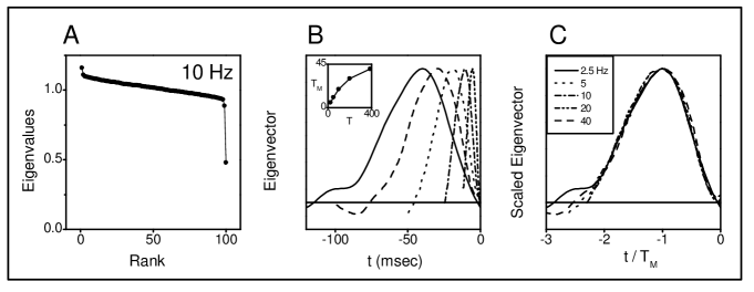
Figure 4: Covariance analysis of the normal form of type I neurons. Spike generation is identified as $\theta$ crossing the angle $\pi$. In all cases, $I_{\rm DC}=-0.01\mu$A/cm², and $\tau=0.2$ ms. A: Eigenvalue spectrum obtained for 10 Hz ($\sigma$ = 0.0046 $\mu$A/cm²ms^1/2, CV = 0.64, 50607 spikes). B: Eigenvectors corresponding to the smallest eigenvalue. Different curves correspond to different firing rates: 2.5 Hz ($\sigma$ = 0.002935 $\mu$A/cm²ms^1/2, CV = 0.81, 51718 spikes), 5 Hz ($\sigma$ = 0.00353 $\mu$A/cm²ms^1/2, CV = 0.73, 49855 spikes), 10 Hz ($\sigma$ = 0.0046 $\mu$A/cm²ms^1/2, CV = 0.64, 50607 spikes), 20 Hz ($\sigma$ = 0.00715 $\mu$A/cm²ms^1/2, CV = 0.60, 49962 spikes), 40 Hz ($\sigma$ = 0.01421 $\mu$A/cm²ms^1/2, CV = 0.57, 50296 spikes). Inset: Time $T_{\rm M}$ at which each eigenvector reaches its maximum value, as a function of the mean inter-spike interval $T$ (the inverse of the firing rate). C: Scaled eigenvectors, for different firing rates. The normal type I model, hence, shows the same qualitative behavior as the conductance-based WB model.

we depict the results of performing a covariance analysis of the normal-form dynamical model of Eq. (2). In A, the eigenvalue spectrum obtained for 10 Hz firing rate is shown. As in the WB model, the most salient eigenvalue is significantly smaller than unity. The largest eigenvalue also seems to depart from unity. We have checked, however, that as one gets closer to threshold (as $I_{\rm DC}\to 0^{-}$), this eigenvalue approaches unity.

Just as it happened with the WB model, near threshold the spectrum of eigenvalues remains essentially unchanged, as the firing rate is varied: in all cases, there is a single eigenvalue significantly smaller than unity. In B, the eigenvector corresponding to this eigenvalue is depicted, for different values of the firing rate. The same qualitative behavior seen in Fig. 3 is obtained: as the firing rate grows, the depolarizing fluctuation in the eigenvector becomes increasingly time-compressed. In the inset of panel B, we show the time $T_{\rm M}$ at which the eigenvector reaches its maximum value, as a function of the mean period $T$ (the inverse of the mean firing rate). In C, the scaled eigenvectors may be seen to fit a fairly universal shape, in spite of the 16-fold variation in the firing rates. Hence, we conclude that the universal behavior observed in the WB model is actually a general property of type I neurons, near threshold.

5 Relevant stimulus features driving type II neurons

In the previous section we saw that type I neurons fire in response to depolarizing stimulus fluctuations, and that those fluctuations lack an intrinsic temporal scale: the faster the stimulus, the higher the firing rate. Here, we explore whether that is also the case for type II neurons. In Fig. 5 we show the results

Figure 5: Covariance analysis of the HH model neuron for two values of the firing rate, for $\tau=0.2$ ms. Upper panels: 10 Hz firing rate ($\sigma=$17.2 $\mu$A/cm²ms^1/2, CV = 0.85, 51165 spikes). Lower panels: 20 Hz firing rate ($\sigma=$22.15 $\mu$A/cm²ms^1/2, CV = 0.69, 51490 spikes). A and D: spectra of eigenvalues. In each case, two outliers are singled out, labeled as a and b. B and E: Time-domain representation of the eigenvectors corresponding to the eigenvalues a and b. C and F: Frequency-domain representation of the eigenvectors a and b.

of carrying out a covariance analysis with the HH model neuron, for two values of the firing rate: 10 Hz (upper panels), and 20 Hz (lower panels). Each spectrum of eigenvalues (A and D) exhibits two outliers, labeled a and b in the figure. The corresponding eigenvectors are depicted in B and E (in the time domain) and in C and F (in the frequency domain). In all cases, the eigenvectors exhibit both positive and negative phases. This result is in agreement with the phase-resetting curves obtained for the supra-threshold HH model (Fig. 2B), suggesting that the relevant subspace comprises characteristic frequencies. For both firing rates, we observe that each eigenvector contains a dominant frequency: eigenvector a peaks at 125 Hz, whereas b reaches its maximum at 62 Hz. As may be easily judged by comparing panels B and E, the temporal domain of the eigenvectors does not seem to contract, as the firing rate is doubled. Accordingly, the principal frequency of each eigenvector (compare C and F) remains unaltered. This means that in the HH model, each eigenvector has a characteristic temporal pattern that is not determined by the firing rate of the cell. A natural question, hence, arises: What governs these temporal patterns and their characteristic frequencies?

To answer this question, we apply covariance-analysis techniques to the reduced model described by Eqs. (4) and (5). In the first place, we choose $c=1$/ms and $f=-1$/ms. More importantly, we fix $\dot{\theta}=\rm{cnst}=2\pi\beta$ (that is, we make $g=d=0$).

Figure 6: Covariance analysis of a normal-form type II neuron model in which the angular velocity $\dot{\theta}$ is independent of the radial coordinate. The bifurcation parameter $\alpha$ is set to -0.5 / ms, and $\tau=0.1$ ms. The noise $\sigma$ is chosen so as to obtain a firing rate of 200 Hz. Upper panels: $\beta=1/$ ms, $\sigma=0.037$ / ms^1/2, CV = 2.3, 48246 spikes. Lower panels: $\beta=0.5$ ms, $\sigma=$ 0.0798 / ms^1/2, CV = 1.3, 49923 spikes. A and E: Dependence of the angular velocity $\dot{\theta}$ on the radial coordinate $r$. B and F: Spectra of eigenvalues. Two almost degenerate outliers are clearly seen. C and G: Eigenvectors in the temporal domain. D and H: Eigenvectors in the frequency domain, plotted in logarithmic scale.

This means that the whole reduced system (4)-(5) revolves with a unique angular velocity $\beta$ around the origin. In Fig. 6, the results obtained for two different values of $\beta$ are shown. In the upper panels, $\beta=1/$ ms, in the lower ones, $\beta=1/$2 ms. In A and E, the dependence of $\dot{\theta}$ with the radial variable $r$ is shown. In B and F, we see the spectra of eigenvalues. In both cases, two almost degenerate eigenvalues (labeled a and b) are significantly smaller than unity. The eigenvectors corresponding to these two eigenvalues are shown in C and G. For each value of $\beta$, the eigenvectors a and b are very similar to each other: they constitute an almost sinusoidal wave-form, of a very well defined frequency. They only differ in a $\pi/2$ phase shift, implying that the relevant stimulus eigenspace is comprised of all linear combinations of a sine and a cosine function, of a specific frequency. The frequency, though, varies with $\beta$. Panels D and H show the power spectra of the two eigenvectors, in logarithmic scale. When $\beta=1/$ms, the maximum power is found at a frequency of 1000 Hz (D), whereas for $\beta=0.5$/ms, the eigenvectors peak at $500$ Hz (H). This means that we are in the presence of a resonance phenomenon: spiking probability is maximized shortly after stimulus segments that contain significant power in the characteristic frequency of the angular motion of the dynamical system.

How do these results change when the angular velocity $\dot{\theta}$ depends on the radial coordinate $r$? This question is pertinent, since type II systems undergo two bifurcations, in two different locations in phase space, and are therefore not amenable of a local reduction. The firing limit cycle appears through a global bifurcation that in principle, may take place far away from the resting fixed point. Hence, the frequency associated to the spiking limit cycle need not coincide with the frequency of subthreshold oscillations. Therefore, in Fig. 7 we

Figure 7: Covariance analysis of a normal-form type II neuron model in which the angular velocity $\dot{\theta}$ either increases with the radial coordinate $r$ (upper panels) or decreases with $r$ (lower panels). The bifurcation parameter $\alpha$ is set to -0.5/ms, and $\tau=0.1$ ms. The noise $\sigma$ is chosen so as to obtain a firing rate of 200 Hz. Upper panels: $\beta=1/$ms, $g=0.5$, $\tau=0.1$ ms, $\sigma=0.025$/ms^1/2, CV = 6.0, 234796 spikes. Lower panels: $\beta=0.5$ms, $g=-0.5$, $\tau=0.1$ ms, $\sigma=0.025$ 0.049/ms^1/2, CV = 1.3, 200212 spikes. A and E: Dependence of the angular velocity $\dot{\theta}$ on the radial coordinate $r$. B and F: Spectra of eigenvalues. Two outliers are clearly seen, one of them (a) with increased variance, the other one (b) with decreased variance. C and G: Eigenvectors in the temporal domain. D and H: Eigenvectors in the frequency domain, plotted in logarithmic scale.

explore the behavior of two other type II systems, where the angular velocity $\dot{\theta}$ either increases with $r$ (upper panels) or decreases with $r$ (lower panels). We see that once the angular velocity $\dot{\theta}$ sweeps over a whole range of frequencies, the degeneracy of the relevant eigenvectors is removed. Actually, now one of the eigenvectors (a) is associated to a direction of increased variance, and the other one (b) corresponds to a diminished variance. Eigenvector b is still centered around the frequency of subthreshold oscillations near the fixed point (that is, 1000 Hz). However, the dominant frequency of eigenvector b has now shifted to a lower or higher value, depending on whether $\dot{\theta}$ is an increasing or decreasing function of $r$. In the upper panels, $\dot{\theta}$ grows with $r$, implying that the firing limit cycle has a higher frequency than the subthreshold oscillations. Correspondingly, the dominant frequency of eigenvector b is shifted to larger values (see D). The lower panels, instead, show a case in which $\dot{\theta}$ is a decreasing function of $r$, and correspondingly, the dominant frequency of eigenvector b has shifted to lower values (see H).

In an arbitrary type II system, the angular velocity may show a rather complicated dependence on the radial coordinate $r$. In consequence, the prototypical system described by Eqs. (4) and (5) contains several non-trivial parameters. The shape of the spectrum of eigenvalues depends rather critically on these parameters, and so do the associated eigenvectors. Actually, by choosing those parameters carefully, it is possible to obtain eigenvalues and eigenvectors that are similar to those of the original HH model. In Fig. (8) we show the results of stimulating the normal form Eqs. (4) and (5) with conveniently selected values of the parameters $\alpha,c,f,\beta,d,g$ so as to obtain an eigenspace that is qualitatively similar to the one generated by the eigenvectors of the HH model of Fig. 5.

Figure 8: Covariance analysis of a normal-form type II neuron model in which the parameters have been chosen in order to obtain two eigenvectors that span a subspace that is qualitatively similar as the one generated by the eigenvectors of the HH model (see Fig. 5). Here, $\tau=0.2$ ms, $c=1.69$/ms, $f=-1.69$/ms, $\beta=0.0477$/ms, $d=-0.0183$/ms, $g=0$, $\alpha=-0.3$/ms, $\sigma=0.028/\rm{ms}^{1/2}$, CV = 0.79, 49409 spikes. The firing rate was 21.0 Hz.

Notice that with these parameters, ${\rm d}\theta/{\rm d}t$ is a decreasing function of $r$. This is in agreement with the behavior of the HH model, where the frequency associated to the firing limit cycle is smaller than the frequency of the subthreshold oscillations around the resting state.

6 Discussion

In this paper, we have analyzed the stimulus features that are relevant in shaping the spiking probability for type I and type II neuron models. Type I models undergo a saddle-node, away-limit-cycle bifurcation at firing onset, and they can be reduced to a normal form that contains a single scale parameter that determines the firing frequency. Our analysis shows that when type I models are stimulated with random input currents whose mean value lies slightly below threshold, they fire in response to depolarizing stimuli. By scaling the relevant eigenvectors obtained from a covariance analysis, we have shown that type I models are not selective to specific temporal scales: the faster the depolarizing input, the faster the neural response.

Previous studies (Agüera y Arcas & Fairhall, 2003) have shown that the firing probability of integrate-and-fire neurons is determined by a 2-dimensional space, spanned by the eigenvectors associated to a small-variance and a large-variance eigenvalues. The eigenvector associated to the small eigenvalue essentially coincided with the eigenvector shown in the type I models of this paper of Sect. 4. The second eigenvector obtained for the integrate-and-fire model, however, combines a hyperpolarizing and a depolarizing phase. In the models studied in Sect. 4, that eigenvector could sometimes be identified (see the largest eigenvalue of Fig. 4). However, as the DC component of the input current approaches the threshold current, the eigenvalue was shown to decrease, until it was hidden in the baseline level of all the other eigenvalues (see Fig. 3). This effect, however, is not found in the integrate-and-fire model, for which all input currents are represented by a spectrum of eigenvalues showing two outliers. Hence, integrate-and-fire neurons do not behave as our prototypical type I neurons. The reason for this discrepancy lies in the fact that near threshold, the slow evolution of integrate-and-fire neurons revolves around the zone of phase space representing the firing threshold. In the type I neuron models discussed in this paper, slow dynamics occurs in the vicinity of the subthreshold resting state. Hence, the two models cannot be mapped onto one another, without the introduction of additional abrupt dynamical features, as the voltage cutoffs employed in Hansel & Mato (2003).

In contrast, type II models are governed by a subcritical Hopf bifurcation, thereby requiring a 2-dimensional, non local description. As a consequence, type II models are characterized by several parameters, that retain various temporal properties of the original dynamical system. These differences between type I and type II neuron models imply that each one of them is responsive to particular features of the input current. Baroni and Varona (2007) have suggested that the differences in the input/output transformation carried out by type I and type II neurons may have evolved to activate different populations of neurons, depending on the specific temporal patterns of the presynaptic input. Muresan and Savin (2007), in turn, have discussed the consequences of these differences at the network level. While type II neurons favor self-sustainability of network activity, type I cells increase the richness of the responsiveness to external stimuli.

The main distinction between the stimulus features driving type I and type II models, as demonstrated by our covariance analysis, provides further justification to the distinction introduced by Izhikevich (2001), where type I neurons are called integrators, and Hopf-like type II neurons are resonators. Our work shows that, indeed, near threshold type I neurons are essentially waiting to receive excitatory input (no matter their time scale), whereas Hopf-like type II neurons are able to detect input segments that contain sufficient power in the frequency band that is well represented by their intrinsic dynamics.

Can the relevant stimulus features be connected to the phase-resetting curves? By comparing Fig. 2 with Fig. 3, we conclude that both the phase-response curve and the preferred stimulus feature of type I neurons (which, as stated above, coincides with the STA) are monophasic and positive. In turn, both the eigenvector corresponding to the smallest eigenvalue of type II neurons (the one that is most similar to the STA) and the phase-response curve exhibit positive and negative phases (compare Figs. 2 and 5). This similarity, however, can only be stated at a qualitative level. Recall that phase-response curves can only be defined in the supra-threshold regime, whereas our the covariance analysis concerned random input currents of subthreshold mean.

Ermentrout, Galán, & Urban (2007) have proved that when a cell is firing regularly while receiving mild random perturbative currents, its spike-triggered average is equal to the temporal derivative of the phase-resetting curve. This result contrasts with our observation that the phase-response curve itself (and not its derivative) has the same sign as the relevant stimulus features inducing spiking, for subthreshold stimuli. The two conclusions, however, are not in conflict with one another. In Fig. 9, the ISI distribution, the STA, and the most relevant eigenvector of a normal-form, type I neuron is shown, when driven with three different stimulation protocols.

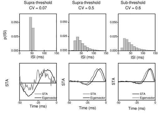
Figure 9: ISI probability densities (upper panels) and most relevant stimulus feature (lower panels) of a normal-form, type I neuron firing at 20 Hz, for three different stimulation protocols. The most relevant stimulus feature is obtained with two different methods: the STA (black line) and the most prominent eigenvector (grey line). Left: Regular firing, with stimuli of supra-threshold mean. $\alpha=0.004$, $\sigma=0.00029$ ms^1/2, $\tau=0.2$ ms, 500159 spikes, CV = 0.07. Middle: Irregular firing, with stimuli of small supra-threshold mean. $\alpha=0.002$, $\sigma=0.00295$ ms^1/2, $\tau=0.2$ ms, 201287 spikes, CV = 0.5. Right: Irregular firing, with stimuli of small sub-threshold mean. $\alpha=-0.001$, $\sigma=0.004345$ ms^1/2, $\tau=0.2$ ms, 49462 spikes, CV = 0.6. When the system is firing regularly (low CV), the STA shows a positive and a negative phase, resembling the derivative of the phase-resetting curve. In contrast, when the system fires in an irregular fashion (large CV), the STA exhibits a large positive phase, and a small negative portion.

The plots on the left correspond to an input stimuli whose mean value is sufficiently large as to keep the system firing regularly at 20 Hz. The noisy component of the injected current, therefore, only rarely modifies the regular spiking pattern, occasionally advancing or delaying an action potential. As a consequence, the inter-spike-interval (ISI) distribution reduces to a very narrow peak located at 50 ms. The STA, in turn, is clearly bi-phasic, and constitutes a very good approximation of the temporal derivative of the phase-resetting curve (see Ermentrout, Galán and Urban, 2007). The most relevant eigenvector is qualitatively similar to the STA, though its shape is noticeably more sensitive to limited sampling.

In order to explore how these results evolve as the activity of the cell becomes more irregular, in the middle and right panels we show the results obtained with other stimulating scheme, where the mean stimulus is lowered, and the stochastic component of the input current is increased as to maintain a 20 Hz firing rate. The ISI distributions are therefore significantly widened. We see that the STA is no longer symmetric with respect to the mean stimulus: the depolarized phase of the STA is markedly larger than the hyperpolarized one. As the mean stimulus is made increasingly negative, the negative phase disappears completely, and the STA merges into the curves shown in Fig. 4. We therefore conclude that the exact relationship between the relevant stimulus features inducing spiking and the phase-response curve depends critically on how regular the spike train is. Which, for fixed firing rate, is governed by the ratio between the SD of the stimulus and its mean value (the CV). We hope that the present analysis may serve to inspire future investigations in the connection between these quantities.

7 Acknowledgements

We thank Eugenio Urdapilleta for useful discussions. This work has been supported by the Comisión Nacional de Investigaciones Científicas y Técnicas (PIP 5140), the Alexander von Humboldt Foundation, the Universidad Nacional de Cuyo and the Agencia Nacional de Promoción Científica y Tecnológica.

Appendix A: Wang Buzsaki (WB) Model

The dynamical equations for the conductance-based type I neuron model used in this work were introduced by Wang and Buzsaki (1996). They are

$$C\frac{{\rm d}V}{{\rm d}t} = I-g_{\rm Na}{\rm m}_{\infty}^{3}(V)h(V-V_{\rm Na})-g_{\rm K}n^{4}(V-V_{\rm K})-g_{\ell}(V-V_{\ell})$$ (12)

$$\frac{{\rm d}h}{{\rm d}t} = \frac{{\rm h}_{\infty}(V)-h}{\tau_{\rm h}(V)}$$ (13)

$$\frac{dn}{dt} = \frac{{\rm n}_{\infty}(V)-n}{\tau_{\rm n}(V)}.$$ (14)

The parameters $g_{\rm Na}$, $g_{\rm K}$ and $g_{\ell}$ are the maximum conductances per surface unit for the sodium, potassium and leak currents respectively and $V_{\rm Na}$, $V_{\rm K}$ and $V_{\ell}$ are the corresponding reversal potentials. The capacitance per surface unit is denoted by $C$. The external stimulus on the neuron is represented by an external current $I$. The functions ${\rm m}_{\infty}(V)$, ${\rm h}_{\infty}(V)$, and ${\rm n}_{\infty}(V)$ are defined as ${\rm x}_{\infty}(V)=a_{\rm x}(V)/[a_{\rm x}(V)+b_{\rm x}(V)]$, where ${\rm x}={\rm m},{\rm n}$ or ${\rm h}$. In turn, the characteristic times (in milliseconds) $\tau_{\rm n}$ and $\tau_{\rm h}$ are given by $\tau_{\rm x}=1/[a_{\rm x}(V)+b_{\rm x}(V)]$, and

$$a_{\rm m} = -0.1(V+35)/(\exp(-0.1(V+35))-1),$$ (15)

$$b_{\rm m} = 4\exp(-(V+60)/18),$$ (16)

$$a_{\rm h} = \phi\,0.07\exp(-(V+58)/20),$$ (17)

$$b_{\rm h} = \phi/(\exp(-0.1(V+28))+1).$$ (18)

The other parameters of the sodium current are: $g_{\rm Na}=35\rm{mS/cm}^{2}$ and $V_{\rm Na}=55\rm{mV}$. The delayed rectifier current is described in a similar way as in the HH model with:

$$a_{n} = \phi\,0.01(V+34)/(1-\exp(-0.1(V+34))),$$ (19)

$$b_{n} = \phi\,0.125\exp(-(V+44)/80).$$ (20)

Other parameters of the model are: $V_{\rm K}=-90\rm{mV},V_{\rm Na}=55\rm{mV},V_{\ell}=-65\rm{mV},C=1\mu\rm{F}/\rm{cm}^{2}$, $g_{\ell}=0.1\rm{mS/cm}^{2},g_{\rm Na}=35\rm{mS/cm}^{2},g_{\rm K}=9\rm{mS/cm}^{2},\phi=3$.

Appendix B: the Hodgkin-Huxley (HH) model

The dynamical equations of the Hodgkin-Huxley (Hodgkin & Huxley, 1952) model read

$$C\frac{{\rm d}V}{{\rm d}t} = I-g_{\rm Na}m^{3}h(V-V_{\rm Na})-g_{\rm K}n^{4}(V-V_{\rm K})-g_{\ell}(V-V_{\ell}),$$ (21)

$$\frac{{\rm d}m}{{\rm d}t} = \frac{{\rm m}_{\infty}(V)-m}{\tau_{\rm m}(V)},$$ (22)

$$\frac{{\rm d}h}{{\rm d}t} = \frac{{\rm h}_{\infty}(V)-h}{\tau_{\rm h}(V)},$$ (23)

$$\frac{{\rm d}n}{{\rm d}t} = \frac{{\rm n}_{\infty}(V)-n}{\tau_{\rm n}(V)}.$$ (24)

For the squid giant axon, the parameters at $6.3\ ^{0}C$ are: $V_{\rm Na}=50\rm{mV}$, $V_{\rm K}=-77$ mV, $V_{\ell}=-54.4\rm{mV}$, $g_{\rm Na}=120\rm{mS/cm}^{2}$, $g_{\rm K}=36\rm{mS/cm}^{2}$ , $g_{\ell}=0.3\rm{mS/cm}^{2}$, and $C=1\mu\rm{F}/\rm{cm}^{2}$. The functions ${\rm m}_{\infty}(V)$, ${\rm h}_{\infty}(V)$, ${\rm n}_{\infty}(V)$, $\tau_{\rm m}(V)$, $\tau_{\rm n}(V)$, and $\tau_{\rm h}(V)$, are defined in terms of the functions $a(V)$ and $b(V)$ as in the WB model, but now

$$a_{\rm m} = 0.1(V+40)/(1-\exp((-V-40)/10)),$$ (25)

$$b_{\rm m} = 4\exp((-V-65)/18),$$ (26)

$$a_{\rm h} = 0.07\exp((-V-65)/20)),$$ (27)

$$b_{\rm h} = 1/(1+\exp((-V-35)/10),$$ (28)

$$a_{\rm n} = 0.01(V+55)/(1-\exp((-V-55)/10)),$$ (29)

$$b_{\rm n} = 0.125\exp((-V-65)/80).$$ (30)

References

1. Agüera y Arcas, B., & Fairhall, A. L. (2003). What causes a neuron to spike? Neural Comput. 15 1789-1807.

2. Agüera y Arcas, B., Fairhall, A. L., & Bialek W. (2003). Computation in Single Neuron: Hodgkin and Huxley Revisited. Neural Comput. 15 1715-1749.

3. Baroni F. & Varona P. (2007). Subthreshold oscillations and neuronal input-output relationships. Neurocomput. 70: 161-1614.

4. Bialek W. & De Ruyter von Steveninck R. R. (2003). Features and dimensions: motion estimation in fly vision. q-bio/0505003.

5. Brown E., Moehlis J., & Holmes P. (2004) On the Phase Reduction and Response Dynamics of Neural Oscillator Populations. Neural Comput. 16 673-715.

6. Ermentrout, B. (1996) Type I Membranes, Phase Resetting Curves, and Synchrony. Neural Comp. 8 979-1001.

7. Ermentrout, B. & Kopell, N. (1986) Parabolic Bursting in an Excitable System Coupled with a Slow Oscillation SIAM Journal on Applied Mathematics 46 233-253.

8. Ermentrout, B., Galán, R., & Urban, N. (2007) Relating neural dynamics to neural coding, arXiv0707:0245v2 [q-bio.NC].

9. Fairhall A., Burlingame C. A., Narasimhan R., Harris R. A., Puchalla J. L. & Berry M. J. (2006). Selectivity for Multiple Stimulus Features in Retinal Ganglion Cells. J. Neurophysiol. 96 2724-2738.

10. Hansel D., Mato G., & Meunier C. (1995). Synchrony in excitatory neural networks. Neural Comput 7 307-337 (1995).

11. Hansel D. & Mato G. (2003) Asynchronous states and the emergence of synchrony in large networks of interacting excitatory and inhibitory neurons. Neural Comput 15 1-56.

12. Hodgkin A. L. (1948). The local electric charges associated with repetitive action in non-medulated axons. J. Physiol. 107 165-181.

13. Hodgkin A. L. & Huxley A. F. (1952) A quantitative description of membrane current and application to conductance in excitation nerve. J. Physiol. (London) 117 500-544.

14. Hong S., Agüera y Arcas B., & Fairhall A. (2007). Single neuron computation: from dynamical system to feature detector. arXiv:q-bio/0612025

15. Izhikevich, E. (2001). Resonate and fire neurons. Neural Networks 14 833-894.

16. Izhikevich, E. (2007). Dynamical Systems in Neuroscience. The Geometry of Excitability and Bursting. The MIT Press.

17. Kuramoto, Y. (2003). Chemical Oscillations, Waves and Turbulence. New York: Dover.

18. Maravall M., Petersen R. S., Fairhall A.L., Arabzadeh E. & Diamond M. E. (2007). Shifts in Coding Properties and Maintenance of Information Transmission during Adaptation in Barrel Cortex. PLoS Biol. 5(2) e19.

19. Muresan R.C. & Savin C. (2007). Resonance or Integration? Self-sustained Dynamics and Excitability of Neural Microcircuits. J. Neurophysiol. 97: 1911-1930.

20. Paninski, L. (2003). Convergence properties of some spike-triggered analysis techniques. Network 14 437-464.

21. Rust N. C., Schwartz O., Movshon J. A, & Simoncelli E. P. (2005) Spatiotemporal Elements of Macaque V1 Receptive Fields. Neuron 46 945-956.

22. Schwartz O., Pillow J. W., Rust N. C. & Simoncelli E. P. (2006). Spike-triggered neural characterization. J. Vision 6 484-507.

23. Wang, X. J., & Buzsáki G (1996) Gamma Oscillation by Synaptic Inhibition in a Hippocampal Interneuronal Network Model. J. Neurosci. 16 6402-6413.