Triplets of Quasars at high redshift I: Photometric data

Abstract

We have conducted an optical and infrared imaging in the neighbourhoods of 4 triplets of quasars. R, z^′, J and K_s images were obtained with MOSAIC II and ISPI at Cerro Tololo Interamerican Observatory. Accurate relative photometry and astrometry were obtained from these images for subsequent use in deriving photometric redshifts. We analyzed the homogeneity and depth of the photometric catalog by comparing with results coming from the literature. The good agreement shows that our magnitudes are reliable to study large scale structure reaching limiting magnitudes of R = 24.5, z^′ = 22.5, J = 20.5 and K_s = 19.0. With this catalog we can study the neighbourhoods of the triplets of quasars searching for galaxy overdensities such as groups and galaxy clusters.

1 Introduction

Our present understanding of galaxy formation and evolution can be improved significantly through studies of quasars. In the unified scenario, merger-driven processes include the origin of a quasar by self-regulating, supermassive, black-hole growth (Hopkins et al., 2005). Thus, most massive spheroids should host an optically-bright quasar during a brief period of its evolutionary history.

There is well-established evidence indicating that several galaxy properties depend on the environment where the galaxies formed and evolved. Several processes - such as stimulated or truncated star formation, tidal stripping, merging, etc. - can determine the nature of galaxy populations and dynamics. Also to be considered is the possibility that AGN feedback processes could induce significant changes in the evolution of galaxies near to the quasar (see for instance Croton et al. (2006)). By studying quasar environments we may deepen our understanding of the relation of quasar fueling and galaxy interactions and merging; and as a consequence, the formation of bright galaxies.

The availability of large quasar samples has increased significantly in recent years, mainly due to the advent of large surveys such as the 2dF Galaxy Redshift Survey (Colless et al., 2001) and the Sloan Digital Sky Survey (Stoughton et al., 2002). These samples provide an opportunity for more robust statistical studies of the quasar phenomenon and its link with galaxy formation.

At low redshifts (z $\leq$ 0.3), existing cross-correlation analysis of quasar environments show that quasars inhabit environments similar to those of normal galaxies (Smith et al. (1995), Coldwell et al. (2002). However, on small scales (projected distance, $r_{p}\leq 1{h^{-1}~{}\rm Mpc}$; and radial velocity difference, $\Delta V=500{\rm km~{}s^{-1}}$), the quasar environment is overpopulated by blue disk galaxies having a strong star-formation rate with respect to typical galaxy neighbourhoods (Coldwell & Lambas, 2003, 2006). This result is in agreement with those of Söchting et al. (2002, 2004) in the sense that low-redshift quasars follow the Large Scale Structure traced by galaxy clusters but they are not located near the center of clusters. These quasars are mainly found in the periphery of such structures or between two, possibly merging, clusters.

At higher redshifts, quasars are often associated with rich environments (Hall & Green, 1998; Djorgovski, 1999) where the comoving density of galaxies is higher than that expected for the general field. This should be interpreted as the core of future rich clusters. Some results at $z\sim 1$ suggest that quasars reside on the peripheries of clusters or in cluster mergers (Haines et al., 2001, 2004; Tanaka et al., 2000, 2001). Tanaka et al. (2001), for example, investigated a group of 5 quasars tracing a $\sim$ 10 Mpc structure of 4–5 clusters, with only a single radio-loud quasar appearing to be directly associated with one of the clusters.

In general, the existing studies of quasar environments suggest their association with forming structures, marking merging clusters and filaments. Consequently, groupings of quasars can be expected to trace regions of extraordinary activity. Pairs of quasars have been strongly studied and they are used to identify cluster of galaxies at high redshifts. Zhdanov & Surdej (2001) suggested that quasar pairs can be used as tracers of high redshift large-scale structures. Moreover, Djorgovski et al. (2003) found a quasar pair at $z\sim 5$ associated with large scale structure, possibly a protocluster at that redshift. More recently, Boris et al. (2007) found that quasar pairs at $z\sim 1$ are excellent tracers of high density environments suggesting that they can be used to find galaxy clusters.

Triplets of quasars in a relative small volume are extremely rare and until now, no cluster-scale triplets have been published or investigated. A very compact quasar association ($\sim$ 50 Kpc separation) was recently reported by Djorgovski et al. (2007) suggesting that this could be a compact galaxy group in a merging process. We propose to use triplets of quasars as “lighthouses” to find and study clusters of galaxies that favour such rare events. With this aim in mind, we performed an optical and infrared photometric study of the environments of triplets of quasars at different redshifts on the scale of galaxy clusters. The images allow us to observe galaxies in the early Universe and they are used to investigate the environments of quasar triplets We also study the group and cluster morphology, and the photometric properties of individual galaxies in the neighbourhood of each triplet. We have already found that low-z triplets of Seyfert 1 galaxies are associated with extremely rich clusters of galaxies (Söchting et al., 2007). If the quasar triggering mechanism does not evolve strongly over redshift we can expect to find some of the richest galaxy clusters ever discovered at $z\sim 1$. A negative result will be clear evidence of the evolution of the quasar formation mechanism.

This paper is organized as follows: In section 2 we describe the sample selection and section 3 shows the optical and infrared observations and data reduction. Section 4 describes the photometric galaxy catalog, and in section 5 we provide a summary of the main results. We adopt the latest cosmology with $\Omega_{M}=0.3$, $\Omega_{\lambda}=0.7$ and a Hubble constant, $H_{0}=70~{}{\rm{km~{}s^{-1}~{}Mpc^{-1}}}$.

2 The Sample

The quasar sample is defined by quasars which have at least one emission line with a full width at half maximum larger than 1000 ${\rm km~{}s^{-1}}$, luminosities brighter than $M_{i}=-23$, PSF $i$ magnitude $<19.1$ and highly reliable redshifts (Schneider et al., 2003). To analyze the regions in the neighbourhoods of groups of quasars, we identified different active systems using the friend-of-friend, three-dimensional, percolation algorithm (Huchra & Geller (1982)). This technique was applied to the sample of 54000 quasars taken from SDSS-DR4 which satisfy the criteria defined above. Taking into account galaxies in clusters and their surroundings, and the low spatial density of quasars (about 15 quasars per square degree), we finally defined as candidates for triplets of quasars those systems with percolation longitudes smaller than 2 ${h^{-1}~{}\rm Mpc}$ and 2000 ${\rm km~{}s^{-1}}$. These limits are about twice the typical region for rich galaxy clusters. We found 293 pairs of quasars, only 7 triplets and no systems with more members. To increase the sample of triplets, we applied the same criteria to the Véron-Cetty & Véron (2003) catalogue.

Figure 1 shows the redshift distribution of the fraction of the quasar number normalized to the total quasar sample, and that corresponding to pairs and triplets (systems) of quasars found with the adopted selection criteria. The redshifts of each of the twelve triplets in the total sample of triplets are marked at the top of the figure. For systems of quasars, there are two peaks at z $\sim$ 0.2 and z $\sim$ 1.8, which are more concentrated than the total quasar sample. In spite of the uncertainties due to the small amount of data for systems of quasars, the presence of these two peaks may be interpreted in terms of differences in the growth of self-regulated black holes for different masses (Di Matteo et al., 2005). They proposed a fast evolutionary growth for the massive black holes formed in the early Universe, which exhausted the surrounding gas due to a higher accretion rate. On the other hand, the lifetime of the active phase increases for black holes of smaller masses implying an excess of low luminosity quasars in the local Universe.

The total sample consists of 12 triplets of quasars: 3 triplets with z $<$ 0.2 and 9 within the range of 0.9 $<$ z $<$ 2.5. As mentioned above, pairs of quasars - as a class - have been extensively studied and so we will concentrate our efforts here only on triplets of quasars, which are very rare.

Our first subsample of triplets of quasars, those nearby triplets with z $<$ 0.2 is discussed in Söchting et al. (2007). Using the photometric and spectroscopic catalogs of the SDSS-DR4, we found a strong association of z $<$ 0.2 triplets with the richest central parts of superclusters. In all cases the individual members of the triplets have been found on the periphery of the main galaxy concentrations.

For some of our second subsample, those triplets at higher redshifts, we performed multicolor photometry of the regions near to these triplets in order to locate associated galaxy groups and clusters.

3 Observations and data reduction

In this paper, we concentrate on four high-redshift triplets from the sample. We obtained multicolor photometry of their neighbourhoods with the CTIO 4m telescope using two instruments: MOSAIC II for the optical and ISPI for the near IR (Proposal Ids. 06A-0146 and 06B-0117). Table 1 shows the observed triplets, including the triplet and quasar identifications, coordinates, redshifts and absolute V magnitudes, respectively.

3.1 Optical imaging

Triplets 5 and 6 were observed in the R and z^′ bands using MOSAIC II during 5 half nights from February 2^nd through 6^th, 2006. This optical instrument is an array of 8 2048 $\times$ 4096 SITe CCDs with a gain of 2 e-/ADU and a scale of 0.27 arcsec/pixel, giving a total field of view of 36 $\times$ 36 arcmin². In the R band, we made eight exposures of 600s for Triplet 5 and eleven exposures of 600s for Triplet 6. Moreover, four exposures of 600s were taken in z^′ band for both triplets. Table 2 shows the triplet Ids together with a summary of the optical observations, in R and z’, in columns 2 and 3, respectively.

3.1.1 Photometry

The images were reduced using the SMSN pipeline (Rest et al., 2005; Garg et al., 2007; Miknaitis et al., 2007) originally created for the SuperMACHO and ESSENCE projects. The SMSN pipeline reduces the raw images using the IRAF mosaic routines XTALK and MSCCMATCH, as well as its own routines in C, perl and python. As part of this reduction, the images are crosstalk corrected, astrometrically calibrated, and split into the 16 separate amplifiers. The images are then bias subtracted and flat fielded. The z-band images were also defringed.

We flux calibrated the R and z^′ images using our observations of several Landolt (1992) and Smith et al. (2002) standard stars, respectively. In our images, point-source magnitudes were obtained using SExtractor (Bertin & Arnouts, 1996) with an aperture diameter of $6\arcsec$, which proved to be adequate by monitoring the growth curve of all the measured stars. For the final calibration, we include the zero point and extinction term. The colour term was negligible compared to magnitude errors and it was not included (as in Gawiser et al. (2006)).

For R magnitudes, the zero point is in agreement with the published value for the instrument. In order to better analyze the precision of our calibration, we also compared the magnitudes of the stars in our fields obtained with SExtractor (MAG_BEST) with the PSF magnitudes computed by SDSS. Before performing the comparison we transformed SDSS r$\arcmin$ magnitudes to our system using Fadda et al. (2004) transformations. Figure 2 shows in the upper panel this comparison of R magnitudes showing the good agreement with those of the SDSS. The mean difference is $\Delta$ R = 0.162 $\pm$ 0.139.

In the z^′-band the comparison with SDSS was made without any transformation because the filters are identical. The bottom panel of Figure 2 shows this comparison. The mean difference is $\Delta$ z^′ = 0.14 $\pm$ 0.08 mag. This offset is consistent with the estimated uncertainty of the overall zero-point, mainly due to the very small number of standard stars used in this band. Our final z^′ magnitudes were corrected by this offset.

We applied the offsets in both bands to correct our final magnitudes. Note also that all magnitudes are in the Vega system.

3.1.2 Astrometric precision

In order to assess the accuracy of the astrometric calibration, we compared the position of the stars in the observed fields with those of the USNO-A2.0 Catalog (Monet et al. 1998). We used only unsaturated stars from our images. Figure 3 shows only the results of the comparison for the z^′-band. The mean offset in the positions between both catalogs is negligible: $\Delta\alpha=-0.057\pm 0.281$ arcsec and $\Delta\delta=-0.097\pm 0.302$ arcsec for R-band and $\Delta\alpha=-0.110\pm 0.236$ arcsec and $\Delta\delta=-0.074\pm 0.302$ arcsec for z^′-band. The scatter in the coordinates is found to be typically smaller than 0.3 arcsec and it is consistent with the astrometric accuracy of the USNO-A2.0 catalog. We also compared the positions of the stars with SDSS sources and we found systematic offsets of 0.218 $\pm$ 0.096 and 0.434 $\pm$ 0.107 in right ascension and declination, respectively - similar to those found by Fadda et al. (2004).

3.2 Infrared imaging

The triplets of quasars were also observed in the infrared using ISPI in two runs during 2006: 5 half nights from April 2^nd to 6^th and 3 complete nights - October 7^th to 9^th. ISPI (Infrared Side Port Imager) is a 1-2.4 $\mu$m imager with an 2048 $\times$ 2048 HgCdTe array with an scale of 0.3 arcsec/pix, giving a field of view of 10.5 x 10.5 arcmin² (van der Bliek et al., 2004). The gain is 4.25 e-/ADU and the dark current is very low - about 0.1 e-/sec for long exposures. However, this array has a number of bad pixels which are located along a few rows and columns in the upper right corner.

All four triplets were observed in the K_s band but only Triplets 6 and 7 were observed in the J band. We used a circular dithering pattern of 15 different positions to observe the triplet fields. For each image in the sequence, the exposure time was 130s $\times$ 1 coadds and 20s $\times$ 5 coadds for J and K_s, respectively. Table 2 includes a summary of the IR observations in columns 2 to 5.

3.2.1 Photometry

For the reduction, we used standard tools in IRAF and some tasks from the CTIO Infrared reduction package (cirred) written by R. Blum for specific ISPI processing. The basic data reduction consisted in creating the master flatfield image from a median of lamps on – lamps off dome flats and the construction of the bad pixel mask. The final master flat was corrected by illumination effects and normalized by the average intensity. Median sky images were created for each dithered sequence. The scientific images were flatfielded, bad pixel corrected, and sky subtracted. The astrometry was performed with the package WCSTools (Mink, 2006). Then for each sequence the images were weighted combined with individual weight map images using SWarp written by E. Bertin .

To calibrate the magnitudes, we observed some standard stars from Persson et al. (1998). We also used those stars in our fields belonging to the 2MASS point source catalog (Cutri et al., 2003) to improve precision. As for the optical magnitudes, the stellar instrumental magnitudes were obtained with an aperture diameter setting of $6\arcsec$. For the final calibration, again we did not include the color term.

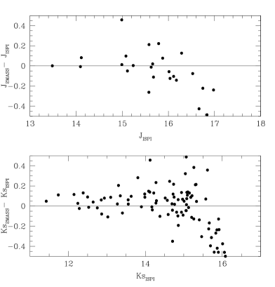
Figure 4: Magnitude comparisons for IR bands between stars in common with 2MASS. Upper and bottom panels show magnitude differences vs our magnitudes for J and Ks bands, respectively.

To verify the photometric precision we compared our magnitudes of detected objects (those with 5 $\sigma$ above the sky background) with the corresponding, uncontaminated, point sources from the 2MASS catalogue. Figure 4 presents comparisons of the magnitude differences for the stars in common with 2MASS in J and K_s bands, respectively; the agreement is excellent. In the J band, for objects brighter than 16 mag, $\Delta J=-0.007\pm 0.153$ mag. In the K_s band, the comparisons look similar; $\Delta K_{s}=-0.066\pm 0.109$ mag for objects brighter than 14.5 mag. Finally, in both bands, we can see from Figure 4 a progressive increase in the scatter at fainter magnitudes due to larger errors in the 2MASS catalogue at these magnitudes.

3.2.2 Astrometric precision

In order to verify the precision of our astrometry, we also checked our measured positions for 2MASS objects in our fields against the 2MASS catalogue. Figure 7 shows the differences in both coordinates, right ascension and declination, between the two sets of data in K_s band. The average differences are $\Delta\alpha=0.096\pm 0.396$ arcsec and $\Delta\delta=0.006\pm 0.347$ arcsec for J band for objects brighter than 16 mag; and $\Delta\alpha=0.038\pm 0.313$ arcsec and $\Delta\delta=0.018\pm 0.371$ arcsec for K_s band for objects brighter than 14.5 mag, an overall astrometric precision sufficient for our purposes.

4 Source detection and catalogue

Our photometric catalog in the four bands was constructed using SExtractor. An object was considered detected if the flux had an excess of 1.5 times the local background noise level over at least 5 connected pixels.

The catalog includes magnitudes in apertures of 2, 3 and 4 arcsec, total magnitudes, star-galaxy separation, ellipticity, etc. The star-galaxy classification represented by the stellarity index, CLASS_STAR allows us to decontaminate the galaxy catalog. Figure 6 shows this parameter as a function of R magnitudes. The results are similar for z^′ band. From the Figure we can see clearly two object sequences: stars defined with CLASS_STAR $\sim$ 1 and galaxies with CLASS_STAR $\sim$ 0. At fainter magnitudes, Bertin & Arnouts (1996) showed that the stellarity index is strongly seeing dependent. Taking this into account, we defined as galaxies those objects with CLASS_STAR $<$ 0.9 and CLASS_STAR $<$ 0.75 for R and z^′ bands, respectively.

The IR photometric catalog was constructed using SExtractor in double-image mode with the K_s image as a reference on account of its better quality.

Figure 7 shows the IR colour-magnitude diagram and how the $J-K_{s}$ colour alone provides a reasonable means of performing the star-galaxy separation. The horizontal sequence at $J-K_{s}<$ 1 corresponds to the stellar sequence of galactic stars with types later than G5 and earlier than K5 (Finlator et al., 2000). In the Figure we also plot point sources detected with CLASS_STAR $>$ 0.95 (star symbols). As can be seen most of these objects are located within the stellar locus box. But those point sources with redder colours ($J-K_{s}>$1 mag and $K_{s}>$ 18) are too faint and the star-galaxy separation becomes unreliable. In spite of this, we prefer to include them in the final catalog (also using star symbols).

To reinforce our star-galaxy separation we also use the half-light radius parameter, $r_{1/2}$. This parameter measures the radius that encloses 50% of the object’s total flux. It is clearly independent of magnitude and depends only of the image seeing. In Figure 8 we show the half-light radius vs $K_{s}$ magnitude. Again, as in Figure 7 point sources with CLASS_STAR $>$ 0.95 are plotted with star symbols. As mentioned in Sub-Section Infrared imaging, there are some bad pixels located along a few rows and columns and yet they were not rejected during the reduction process. These objects have $r_{1/2}<$ 1 in the Figure and they were discarded in the final catalog. Also, the stellar locus is clearly visible at $r_{1/2}\sim$ 2 and $K_{s}<$ 18. Therefore, we define as galaxies those objects with $J-K_{s}>$ 1 and $K_{s}<$ 18 mag.

We created the final photometric catalog discarding spurious objects and stars.

4.1 Results. Number counts

The final catalog in all bands was obtained with total magnitudes, and no need to apply an aperture correction. Our fields are located at $\mid b\mid>40$°, so the Galactic extinction effect is generally small. Only the R magnitudes were corrected for galactic extinction using the $E(B-V)$ values provided in the NASA / IPAC Extragalactic Database (NED) , which are based on the $E(B-V)$ values from the extinction maps of Schlegel et al. (1998).

The number counts as a function of magnitude allow us to analyze the homogeneity and depth of the catalog and to compare it with results obtained from the literature.

Table 3 shows the main result, the number of galaxies per square degree per magnitude in the four bands: R, z^′, J and K_s and their respective errors. The Figures 9, 10, 11 and 12 show the galaxy number counts, in the four bands. We compared our results with galaxy number counts from the literature, mainly: MacDonald et al. (2004) and Metcalfe et al. (2001) in the R band; Kashikawa et al. (2004) and Capak et al. (2004) in the z^′ band; Olsen et al. (2006), Saracco et al. (1999) and Iovino et al. (2005) for the J band; and finally Best et al. (2003), Olsen et al. (2006), Best (2000) and Bornancini et al. (2004) for K_s band. From these Figures it is clear that we reach magnitudes of R = 24.5 mag, z^′ = 22.5 mag, J = 20.5 mag and K_s = 19.0 mag. Within these limiting magnitudes, we find good agreement with the galaxy counts coming from other authors in all bands.

5 Summary

We selected a sample of triplets of quasars as those triple systems with percolation longitudes smaller than 2 ${h^{-1}~{}\rm Mpc}$ and 2000 ${\rm km~{}s^{-1}}$. The goal is to use them as “lighthouses” to find richest clusters. For this purpose we conducted a photometric study of the neighbourhoods of 4 triplets of quasars in the redshift range of 0.9 to 1.7. Images in R, z^′, J and K_s bands were obtained with MOSAIC II and ISPI at CTIO. Magnitudes and coordinates were found to be in excellent agreement with the USNO-A2.0 and 2MASS catalogs. We analyzed the homogeneity and depth of the photometric catalog by comparing the number counts with results coming from the literature. The excellent agreement shows that our magnitudes are reliable, down to limiting magnitudes of R = 24.5, z^′ = 22.5, J = 20.5 and K_s = 19.0. These results allow us to study large- scale structure and in a forthcoming paper we will deal with the statistical analysis of this data.

6 Acknowledgments

This research was partially supported by grants from CONICET, Agencia Córdoba Ciencia and the Secretaría de Ciencia y Técnica de la Universidad Nacional de Córdoba. GVC would like to thank the CTIO for hospitality during her observational runs. IKS would like to acknowledge the kind hospitality of the IATE group during her stay at Cordoba. We would also like to thank Roger Clowes for sharing with us his fringe frames for MOSAIC data. This publication makes use of data products from the Two Micron All Sky Survey, which is a joint project of the University of Massachusetts and the Infrared Processing and Analysis Center/California Institute of Technology, funded by the National Aeronautics and Space Administration and the National Science Foundation. Also, the authors make use of the NASA/IPAC extragalactic database (NED) which is operated by the Jet Propulsion Laboratory, Caltech, under contract with the National Aeronautics and Space Administration.

Table 1: The Observed Sample of Triplets of Quasars

Triplet	RA(J2000)	DEC(J2000)	z	MV
Quasar Id.
TRIPLET 4
2QZ J015646-2828	1:56:46.6	-28:28:0	0.919	-24.5
2QZ J015647-2831	1:56:47.9	-28:31:43	0.919	-24.4
2QZ J015656-2823	1:56:56.0	-28:23:35	0.925	-24.3
TRIPLET 5
SDSS J10023+0155	10:02:19.5	01:55:37	1.509	-24.8
SDSS J10025+0150	10:02:34.3	01:50:10	1.506	-25.7
SDSS J10026+0159	10:02:36.7	01:59:48	1.516	-24.7
TRIPLET 6
2QZ J120914+0035	12:09:14.9	00:35:51	1.316	-25.8
2QZ J120919+0029	12:09:19.6	00:29:26	1.319	-24.3
2QZ J120922+0026	12:09:22.4	00:26:46	1.322	-24.2
TRIPLET 7
2QZ J235405-2845	23:54:05.3	-28:45:06	1.673	-25.2
2QZ J235430-2848	23:54:30.2	-28:48:41	1.670	-24.6
2QZ J235414-2848	23:54:14.2	-28:48:10	1.679	-25.8

Table 2: Observing Logs

Triplet Id.	R	z′	J	Ks
TRIPLET 4	–	–	–	7 $\times$ 15 $\times$ 5 $\times$ 20s
TRIPLET 5	8 $\times$ 600s	4 $\times$ 600s	–	8 $\times$ 15 $\times$ 5 $\times$ 20s
TRIPLET 6	11 $\times$ 600s	4 $\times$ 600s	15 $\times$ 15 $\times$ 130s	8 $\times$ 15 $\times$ 5 $\times$ 20s
TRIPLET 7	–	–	12 $\times$ 15 $\times$ 130s	7 $\times$ 15 $\times$ 5 $\times$ 20s

Table 3: Number Counts in N Deg^-1 0.5 Mag^-1

Magnitude	R	z′	J	Ks
14.75	…	…	…	126 $\pm$63
15.25	…	…	…	347 $\pm$104
15.75	…	…	…	663 $\pm$144
16.25	…	…	410 $\pm$113	1359 $\pm$207
16.75	…	…	726 $\pm$151	2117 $\pm$258
17.25	…	151 $\pm$21	979 $\pm$175	4013 $\pm$356
17.75	…	281 $\pm$29	2180 $\pm$262	5466 $\pm$415
18.25	…	446 $\pm$36	2054 $\pm$254	10110 $\pm$565
18.75	…	814 $\pm$49	4013 $\pm$356	13680 $\pm$657
19.25	357 $\pm$32	1489 $\pm$66	6098 $\pm$438	15580 $\pm$701
19.75	804 $\pm$48	2269 $\pm$81	7520 $\pm$487	15580 $\pm$701
20.25	1416 $\pm$64	3827 $\pm$105	11630 $\pm$606	13020 $\pm$641
20.75	2112 $\pm$78	5946 $\pm$131	12950 $\pm$639	5814 $\pm$428
21.25	2945 $\pm$92	8487 $\pm$157	13110 $\pm$643	…
21.25	2945 $\pm$92	8487 $\pm$157	9826 $\pm$557	…
21.75	4599 $\pm$116	14490 $\pm$205	6667 $\pm$459	…
22.25	6754 $\pm$140	18820 $\pm$233	…	…
22.75	10340 $\pm$173	17250 $\pm$224	…	…
23.25	16160 $\pm$217	10180 $\pm$172	…	…
23.75	26070 $\pm$275	…	…	…
24.25	37260 $\pm$329	…	…	…
24.75	40550 $\pm$343	…	…	…
25.25	11050 $\pm$179	…	…	…

Figure 1: Relative redshift distribution of the total quasar sample (dashed line), and systems of quasars represented by pairs and triplets (solid line). The redshifts of the 12 triplets in our sample are marked at the top of the figure.

Figure 2: Magnitude comparisons for optical bands between stars in our observed fields and those stars in common with SDSS. Upper panel shows the R-band magnitude differences before applying Fadda et al (2004) transformation to SDSS r$\arcmin$ magnitudes. Bottom panel shows the z^′-band magnitude differences.

Figure 3: Astrometric differences in coordinates between the matched MOSAIC II and USNOA2.0 stars in the z^′-band.

Figure 5: Differences in right ascension and declination of stars in common with the 2MASS catalog in the K_s band.

Figure 6: The star-galaxy separation versus total magnitudes for R band.

Figure 7: IR Color–magnitude diagram to discriminate among stars and galaxies. Star symbols correspond to those objects with CLASS_STAR $>$ 0.95.

Figure 8: Half-light radius vs $K_{s}$ magnitude. As in previous Figure, star symbols correspond to those objects with CLASS_STAR $>$ 0.95. The vertical line marks our detectability limit.

Figure 9: Number counts N(R) in the R band. We also show number counts coming from other authors: MacDonald et al. (2004) and Metcalfe et al. (2001).

Figure 10: Number counts N(z^′) in the z^′ band. We also show number counts coming from other authors: Kashikawa et al. (2004) and Capak et al. (2004).

Figure 11: Number counts N(J) in the J band. We also show number counts coming from other authors: Olsen et al. (2006), Saracco et al. (1999) and Iovino et al. (2005).

Figure 12: Number counts N(K_s) in the K_s band. We also show number counts coming from other authors: Best et al. (2003), Olsen et al. (2006), Best (2000) and Bornancini et al. (2004).

References

- Bertin & Arnouts (1996) Bertin E., Arnouts S.,1996, A & A Supp. 117, 393.
- Best (2000) Best, P. N. 2000, MNRAS, 317, 720
- Best et al. (2003) Best, P. N., Lehnert, M. D., Miley, G. K., Röttgering, H. J. A. 2003, MNRAS, 343, 1
- Boris et al. (2007) Boris, N. V., Sodré, L., Jr., Cypriano, E. S., Santos, W. A., de Oliveira, C. M., & West, M. 2007, ApJ, 666, 747
- Bornancini et al. (2004) Bornancini, C. G., Martínez, H. J., Lambas, D. G., de Vries, W., van Breugel, W., De Breuck, C., & Minniti, D. 2004, AJ, 127, 679
- Capak et al. (2004) Capak, P., et al. 2004, AJ, 127, 180
- Coldwell et al. (2002) Coldwell, G. V., Martínez, H. J., & Lambas, D. G. 2002, MNRAS, 336, 207
- Coldwell & Lambas (2003) Coldwell, G. V., & Lambas, D. G. 2003, MNRAS, 344, 156
- Coldwell & Lambas (2006) Coldwell, G. V., & Lambas, D. G. 2006, MNRAS, 371, 786
- Colless et al. (2001) Colless, M., et al. 2001, MNRAS, 328, 1039
- Croton et al. (2006) Croton, D. J., et al. 2006, MNRAS, 365, 11
- Cutri et al. (2003) Cutri, R. M., et al. 2003, The IRSA 2MASS All-Sky Point Source Catalog, NASA/IPAC Infrared Science Archive. http://irsa.ipac.caltech.edu/applications/Gator/
- Di Matteo et al. (2005) Di Matteo, T., Springel, V., & Hernquist, L. 2005, Nature, 433, 604
- Djorgovski (1999) Djorgovski, S. G. 1999, The Hy-Redshift Universe: Galaxy Formation and Evolution at High Redshift, 193, 397
- Djorgovski et al. (2003) Djorgovski, S. G., Stern, D., Mahabal, A. A., & Brunner, R. 2003, ApJ, 596, 67
- Djorgovski et al. (2007) Djorgovski, S. G., Courbin, F., Meylan, G., Sluse, D., Thompson, D., Mahabal, A., & Glikman, E. 2007, ApJ, 662, L1
- Fadda et al. (2004) Fadda, D., Jannuzi, B. T., Ford, A., & Storrie-Lombardi, L. J. 2004, AJ, 128, 1
- Finlator et al. (2000) Finlator, K., et al. 2000, AJ, 120, 2615
- Garg et al. (2007) Garg, A., et al. 2007, AJ, 133, 403
- Gawiser et al. (2006) Gawiser, E., et al. 2006, ApJS, 162, 1
- Haines et al. (2001) Haines, C. P., Clowes, R. G., Campusano, L. E., & Adamson, A. J. 2001, MNRAS, 323, 688
- Haines et al. (2004) Haines, C. P., Campusano, L. E., & Clowes, R. G. 2004, A&A, 421, 157
- Hall & Green (1998) Hall, P. B., & Green, R. F. 1998, ApJ, 507, 558
- Hopkins et al. (2005) Hopkins, P. F., Hernquist, L., Cox, T. J., Di Matteo, T., Martini, P., Robertson, B., & Springel, V. 2005, ApJ, 630, 705
- Huchra & Geller (1982) Huchra, J. P., & Geller, M. J. 1982, ApJ, 257, 423
- Iovino et al. (2005) Iovino, A., et al. 2005, A&A, 442, 423
- Kashikawa et al. (2004) Kashikawa, N., et al. 2004, PASJ, 56, 1011
- Landolt (1992) Landolt, A. U. 1992, AJ, 104, 340
- MacDonald et al. (2004) MacDonald, E. C., et al. 2004, MNRAS, 352, 1255
- Metcalfe et al. (2001) Metcalfe, N., Shanks, T., Campos, A., McCracken, H. J., & Fong, R. 2001, MNRAS, 323, 795
- Miknaitis et al. (2007) Miknaitis, G., et al. 2007, ApJ, 666, 674
- Mink (2006) Mink, D. 2006, ASP Conf. Ser. 351: Astronomical Data Analysis Software and Systems XV, 351, 204
- Monet et al. (1998) Monet, D., Canzian, B., Harris, H., Reid, N., Rhodes, A., & Sell, S. 1998, VizieR Online Data Catalog, 1243, 0
- Olsen et al. (2006) Olsen, L. F., et al. 2006, A&A, 456, 881
- Persson et al. (1998) Persson, S. E., Murphy, D. C., Krzeminski, W., Roth, M., & Rieke, M. J. 1998, AJ, 116, 2475
- Rest et al. (2005) Rest, A., et al. 2005, ApJ, 634, 1103
- Saracco et al. (1999) Saracco, P., D’Odorico, S., Moorwood, A., Buzzoni, A., Cuby, J.-G., & Lidman, C. 1999, A&A, 349, 751
- Schlegel et al. (1998) Schlegel, D. J., Finkbeiner, D. P., & Davis, M. 1998, ApJ, 500, 525
- Schneider et al. (2003) Schneider, D. P., et al. 2003, AJ, 126, 2579
- Smith et al. (1995) Smith, R. J., Boyle, B. J. & Maddox, S. J., 1995, MNRAS, 277, 270.
- Smith et al. (2002) Smith, J. A., et al. 2002, AJ, 123, 2121
- Söchting et al. (2002) Söchting, I. K., Clowes, R. G., & Campusano, L. E. 2002, MNRAS, 331, 569
- Söchting et al. (2004) Söchting, I. K., Clowes, R. G., & Campusano, L. E. 2004, MNRAS, 347, 1241
- Söchting et al. (2007) Söchting, I. K., Coldwell, G. V., Alonso, M. V., Smith, M. & Lambas, D. G. 2007, in preparation
- Stoughton et al. (2002) Stoughton, C., et al. 2002, AJ, 123, 485
- Tanaka et al. (2000) Tanaka, I., Yamada, T., Aragón-Salamanca, A., Kodama, T., Miyaji, T., Ohta, K., & Arimoto, N. 2000, ApJ, 528, 123
- Tanaka et al. (2001) Tanaka, I., Yamada, T., Turner, E. L., & Suto, Y. 2001, ApJ, 547, 521
- van der Bliek et al. (2004) van der Bliek, N. S., et al. 2004, SPIE–The International Society for Optical Engineering, 5492, 1582
- Véron-Cetty & Véron (2003) Véron-Cetty, M.-P., & Véron, P. 2003, A&A, 412, 399
- Zhdanov & Surdej (2001) Zhdanov, V. I., & Surdej, J. 2001, A&A, 372, 1