Inter–areal coordination of
columnar architectures during
visual cortical development

The occurrence of a critical period of plasticity in the visual cortex has long been established, yet its function in normal development is not fully understood. Here we show that as the late phase of the critical period unfolds, different areas of cat visual cortex develop in a coordinated manner. Orientation columns in areas V1 and V2 become matched in size in regions that are mutually connected. The same age trend is found for such regions in the left and right brain hemisphere. Our results indicate that a function of critical period plasticity is to progressively coordinate the functional architectures of different cortical areas - even across hemispheres.

Sensory input has the capacity to shape neuronal circuits, especially in the juvenile brain. In the visual cortex, the period when circuits are particularly susceptible to changes of visual input typically lasts many weeks as highlighted by the critical period for the effects of monocular deprivation (?, ?, ?). The onset of this period is delayed relative to the onset of visual experience (?, ?, ?) and key response properties of neurons are already present in almost adult form well before critical period onset (?, ?). What then is the function of a period of relatively strong plasticity at such a late stage of development? Evidently, it enables the cortex to adapt to deprivations from visual input (?, ?, ?) that may be caused by injuries or disease or, under normal conditions, by the shadows of retinal blood vessels (?). By the same token, however, short periods of abnormal vision can cause permanent deficits. The paradox of the critical period of plasticity is, thus, that it seems to provide only little benefit compared to its great potential for handicap (?). Alternatively, it has often been suggested that a period of plasticity plays an important role for the development of normal vision by refining neural circuits through structured patterns of cortical activity. In fact, under normal experience, vision improves during this period (?), but no evidence for a reorganization of visual cortical representations has been observed so far (?, ?).

Here, we show that in cat visual cortex columnar architectures of different cortical areas develop in a coordinated manner as the late phase of the period of plasticity unfolds. Orientation columns analyzing contours in different parts of the visual field constitute a repetitive structure in visual cortical areas V1 and V2 (?, ?) (Fig. 1, A and B). Orientation columns in animals aged between 6 and 15 weeks were labeled with 2-[¹⁴C]-deoxyglucose (2-DG) (?) and visualized in flat-mount sections of cat visual cortical areas V1 and V2  (?, ?, ?) (n=41 brain hemispheres; N=27 animals). Both V1 and V2 contain a complete topographic representation of the contralateral visual field (?, ?). Columns at topographically corresponding locations in the two areas represent similar visual field positions and are selectively and mutually connected by corticocortical connections (?). This topography of the two areas enables us to conveniently compare the layout of distant columns that are mutually connected and represent related aspects of the sensory input. We analyzed the spacing of orientation columns locally using a recently developed wavelet method (?). Because this method provides highly precise estimates of local column spacing with an error much smaller than the large intrinsic variability (?, ?) of column spacings (SEM, 15–50$\mu$m), differences and similarities of column spacings in the sample can be identified reliably.

We first analyzed the mean spacing of orientation columns in areas V1 and V2 and assessed their statistical and age dependence. We found that mean column spacings, $\Lambda$, varied considerably in different individuals (Fig. 1C). In V1 values ranged between 1.1mm and 1.4mm, in V2 between 1.2mm and 1.8mm. The distributions for the two areas were partially overlapping with the smallest column spacings from V2 at about the average value of V1. Nevertheless, in all hemispheres, the mean column spacing, $\Lambda$, in V2 was substantially larger than in V1, consistent with previous reports (?). Mean column spacings, $\Lambda$, did not vary independently across different animals in V1 and V2, but were substantially correlated in both areas (Fig 1D; r=0.62, p$<10^{-5}$, permutation test). A dependence on the age of animals, however, was not observed, neither for mean column spacings, $\Lambda$, (see also Fig. 5F) nor for their differences between V1 and V2 (data not shown).

An age dependence of column spacings became apparent, when we decomposed the spatial variation and covariation of column spacings in areas V1 and V2 into different components. In both areas V1 and V2, orientation columns generally exhibited a substantial intra-areal variation in spacing around the mean column spacing. One part of this variation is common to all hemispheres. In the following, we will call this the systematic topographic component of column spacings (the blue map in the supplementary Fig. S1). It is the intra-areal variation (in V1 or V2) averaged over the entire population of hemispheres, thus it is a 2D spacing map with zero mean. For averaging, the V1/V2 borders of different hemispheres were aligned and maps from right hemispheres were mirror-inverted. The remaining component of variation characterizes an individual hemisphere and is called individual topographic component of column spacings in the following (the orange map in Fig. S1). It is also a 2D spacing map with zero mean calculated by subtracting from the map of local column spacing of an area its mean and the systematic component. The variances of the systematic component, of the individual topographic component, and of the mean column spacing add up to the total variance of local column spacings in the sample. The individual topographic component accounted for the largest part of the variance of column spacings in both areas V1 and V2 (Supplementary Fig. S1D). As shown below examining this bigest variance component reveals that column sizes at topographically corresponding locations in different areas become better matched as the critical period progresses. First, however, we will examine the systematic component which demonstrates that orientation columns in the two areas are coordinated on average.

In V1, the systematic component exhibited virtually the same overall 2D organization as the one in V2, appearing as a horizontally stretched mirror-image of the V2 map when displayed side by side (Fig. 2, A and B). The systematic variation in areas V1 and V2 ranged between -0.15mm and +0.15mm (Fig. 2, A and B). In both areas, columns were systematically wider than average along the representation of the horizontal meridian (HM) with this tendency increasing towards the periphery. In contrast, columns smaller than average prevailed along the peripheral representations of the vertical meridian (VM). In order to conveniently compare topographically corresponding parts in areas V1 and V2, the V2 map was mirror-inverted and morphed by superimposing major landmarks such as the representations of the VM (located along the V1/V2 border), the central visual field, and the HM. The morphed V2 map strongly resembled the V1 map (compare Fig. 2, B and C), and the cross-correlation between the maps was high (r=0.66). Furthermore, the systematic component observed in a comparable data set of ocular dominance column spacings in cat V1 (Fig. 2D, modified from (?)) also exhibited a very similar intra-areal organization with a strong cross-correlation of r=0.82 to the population averaged spacing map for orientation columns in V1 (compare Fig. 2, B and D). No significant age dependence was found for the systematic component of column spacings when calculated separately for groups of younger and older animals.

Next, we analyzed the individual topographic component of local column spacings. Like the systematic component, the individual topographic component was often similar in V1 and V2 in regions analyzing the same part of the visual field and being mutually connected. The examples shown in Fig. 3, A to C, display the same general pattern in both areas V1 and V2 with maxima (white) and minima (dark orange) at approximately corresponding retinotopic locations. More examples are shown in Supplementary Fig. S2. Among different brains the pattern of individual component differed considerably. To quantify the similarity of the individual topographic component in V1 and V2 we calculated, for each hemisphere, the absolute value of the difference between both maps averaged over all analyzed locations, called their mismatch $\Delta_{{V1V2}}$. These mismatches, $\Delta_{{V1V2}}$, were significantly smaller than values obtained for randomly assigned pseudo V1/V2 pairs (p=0.03, permutation test). Thus, in an individual hemisphere the individual topographic component is coordinated at topographically corresponding locations of both areas.

Intriguingly, this column size matching also applied to columns at corresponding locations in left right pairs of areas from both hemispheres. Whereas maps of the individual topographic component in pairs of both hemispheres differed at mirror-symmetric locations, they were often very similar along the V1/V2 border, i.e. in the region containing the cortical representations of the VM (Fig. 3E). V1-columns of representations of the VM in both hemispheres receive similar afferent input and also mutual input mediated by callosal connections concentrated in the vicinity of the VM representation (?, ?). By the mismatch, $\Delta_{LR}$, we quantified the absolute value of differences between left and right maps averaged over a strip of 3mm width adjacent to the V1/V2 border. Values of $\Delta_{LR}$ were significantly smaller than those obtained for randomly assigned pairs of hemispheres, (p=0.01, permutation test). A similar behavior was found for V2 (data not shown). Missmatches $\Delta_{LR}$ were larger for regions more distant from the V1/V2 border.

Analyzing the dependency of column size matching on age, we found that it improves between different areas during the late phase of the critical period. Examples are shown in Fig. 4, A and B. Whereas in younger animals the pattern of individual topographic component differed in V1 and V2 (Fig. 4A) and along the V1/V2 border (Fig. 4B), it was relatively similar in older animals. Fig. 4, C to E, shows the column spacing mismatches $\Delta$ for topographically corresponding columns in V1/V2 pairs and in left/right pairs of V1 and of V2 as a function of age. For all three pairs of areas substantial mismatches were only observed in animals younger than 10 weeks. In older animals mismatches of column spacing were in general less than 0.1mm. Consequentially, all three measures were significantly anti-correlated with animal age ($\Delta_{V1V2}$, $r=-0.39$, $p=0.01$; $\Delta_{LR}$ for V1, $r=-0.64$, $p=0.007$; for V2, $r=-0.50$, $p=0.02$). In contrast, the average column spacing in areas V1 and V2 was independent of age (Fig. 4F). Thus, whereas the average column spacing in areas V1 and V2 remained constant, locally, the column spacing increased or decreased such that mutually connected columns in different areas became coordinated in size.

Previous studies emphasized the apparent stability of the columnar architecture during early visual development (?, ?). Unlike these studies, but fully consistent with them, we observe changes of the columnar architecture during the late phase of the period of visual cortical plasticity. Assessed by monocular deprivation, the critical period peaks at postnatal week 6 and slowly decreases afterward (?, ?). In addition, both the connections from V1 to V2 and the callosal connections undergo a process of refinement over this age range. Densities of connections are maximal between week 4 and week 10 and then gradually decline over the following months (?, ?). We observed changes in three pairs of visual areas, in the two areas V1 from the left and right brain hemispheres, in the two areas V2, and in areas V1 and V2 from the same hemisphere. The changes involve large parts of each of these areas and result in refined coordination of column sizes among mutually connected regions.

The trend to minimize the mismatch of column sizes between different areas suggests a process of optimization of columnar architectures that is not confined to individual areas, but potentially spans the entire visual system. Known mechanism may underlay the emergence of coordinated column layouts in widely distributed cortical regions. Recently, it has been shown that pharmacologically shifting the balance of inhibition and excitation during development modifies column spacing in cat V1 (?). Presumably, column spacings are also determined by the local inhibitory-excitatory balance in normal development. Here this balance may be set by regulatory mechanisms such as synaptic scaling (?), that are sensitive to neuronal activity. The emergence of size matched columns in distant cortical regions might thus be caused by a similar balance of inhibition and excitation in these regions that emerges from their mutual synaptic coupling. Because cortical processing in general takes place in networks distributed across many areas, it is conceivable that developing matching of local circuits serving different submodalities is a general characteristic of cortical network formation.

• We thank M. Puhlmann and S. Bachmann for excellent technical assistance; U. Ernst for providing the morphing program; W. Singer for his permission to use the 2-DG autoradiographs obtained by S.L. in his laboratory for quantitative analysis; T. Geisel for fruitful discussions; M. Brecht, D. Brockmann and S. Palmer for helpful comments on an earlier version of this manuscript. Supported by MPG, HSFP.

Supporting Material
Materials and Methods
References
Fig. S1, S2
Table S1

Fig. 1. Mean column spacings in V1 and V2 covary. (A) and (B) Overall layout of orientation columns in V1 and V2 in two individuals (white dashed line: V1/V2 border; scale bar, 10mm). For A the mean column spacing $\Lambda$ is relatively large in both areas (V1, 1.21mm; V2, 1.58mm), whereas for B it is small in both areas (V1, 1.09mm; V2, 1.31mm). (C) Mean column spacings $\Lambda$ in V1 (crosses) and V2 (boxes) from n=41 hemispheres (N=27 animals). Values in V1 and V2 vary considerably in different hemispheres (V1, 1.0–1.4mm; V2, 1.2–1.8mm). (D) Mean column spacings $\Lambda$ in V1 and V2 are strongly correlated (r=0.62, p$<10^{-5}$, permutation test).

Fig. 2. The systematic topographic component of column spacing is similar in subregions encoding the same visual field position in areas V1 and V2. (A and B) Systematic topographic component of orientation column spacing in V2 (A) and V1 (B) (color scale codes systematic deviation from the mean value; arrangement and symbols as in Fig. 1). (C) The morphed map from V2 (A). (D) Population averaged spacing of ocular dominance columns in cat V1 (modified from  (?). SD for V2, 0.052mm; V1, 0.047mm; V1 ocular dominance columns, 0.049mm. Scale bar, 10mm. Note that for both orientation and ocular dominance maps columns representing the HM and, in particular, the horizontal periphery were on average wider than columns representing the peripheral parts of the VM. Hence, the systematic variations of orientation columns in V1 and V2 were correlated at topographically corresponding locations (correlation between (B) and (C), r=0.69), as were those of orientation and ocular dominance columns in V1 (correlation between (B) and (D), r=0.82).

Fig. 3. In individual brains, columns in different areas are closely matched in size at topographically corresponding subregions. (A-C) Similarity of the individual topographic component of column spacings in V1 and V2. (A) The overall layout of orientation columns for the hemisphere shown in Fig. 1. A pair of topographically corresponding subregions from the more anterior part of V1 and V2 (yellow boxes) and a pair from the more posterior part (blue boxes) are displayed magnified such that all differences but the individual variation were equalized. The relative difference of mean column spacings in V1 and V2 was $\Lambda_{V2}/\Lambda_{V1}=1.3$. To equalize this difference, the subregions from V1 were magnified relative to those from V2 by this factor. To equalize the differences due to the systematic topographic component the two posterior sub-regions were magnified by an additional factor of $1.05$. Note that the spacing of columns is similar within each pair. (B) Patterns of individual variation of column spacing for V2, V1, and the morphed version of V2 for the hemisphere in (A) (color scale, black cross and contour lines as in Fig. 1). (C) Similarity of the individual variation in V1 and V2 at topographically matched locations in another example. (D and E) Similarity of the individual topographic component of column spacings in the left and right brain hemisphere. (D) The overall layout of orientation columns in the left and right hemisphere of an individual animal. A pair of topographically corresponding regions from the anterior part of the VM representation in V1 of both hemispheres (yellow boxes) and a pair from a more posterior part in V1 (blue boxes) was magnified such that all differences except the individual topographic component were equalized. Mean column spacings $\Lambda_{V1}^{r}$ and $\Lambda_{V1}^{l}$ were equal in both hemispheres and the systematic topographic components were equalized by magnifying the two posterior sub-regions by a factor $0.98$. Note that the spacing of columns is similar within each pair. (E) Patterns of the individual variation of local column spacing in V1 for the hemispheres in (D) displayed with the representation of the VM side by side (crosses and contour lines as in Fig. 1). In both residual maps, the blue rectangles (width, 3mm) are positioned at the representation of the VM. Note that the residual maps tend to be similar only along the VM-representations. Scale bar, 10mm.

Fig. 4. Consolidation of column size matching with age. (A and B) Comparison of individual topographic component of column spacing in V1/V2 pairs (A) and in left/right pairs from V1 (B) at earlyer and later ages. (C) Distances $\Delta_{{V1V2}}$ between the individual topographic components in V1 and V2 versus age. (D) Distances $\Delta_{LR}$ between the V1 individual topographic components in the left and right brain hemispheres versus age (calculated within the blue rectangles in B). (E) Distances $\Delta_{LR}$ for V2 (calculated in the blue rectangles in B from the morphed maps of V2). (F) Mean column spacings $\Lambda$ in V1 (crosses) and V2 (boxes) (from Fig. 1C) versus age. Correlations with age are significant in (C) ($r$=-0.64, p=0.007), (D) ($r$=-0.5, p=0.02) and (E) ($r$=-0.39, p=0.01), but were not significant in (F) (p 0.05).

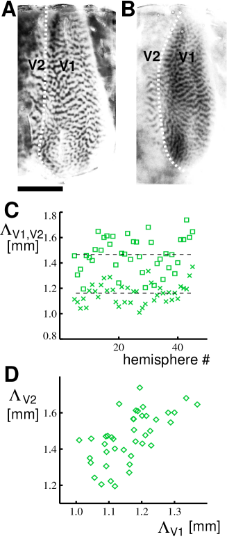
Figure 1:

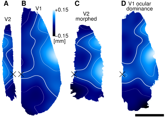
Figure 2:

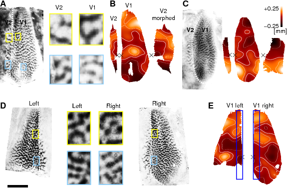
Figure 3:

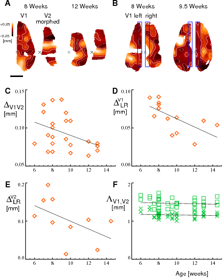
Figure 4:

Supplementary Material

Materials and Methods.

First, we provide an overview over the calculation of local column spacing and its decomposition into its three components analyzed in the manuscript. In more detail, this is outlined in the remainder of the supplement.

Decomposition of orientation column spacing. We analyzed the spacing of orientation columns in cat V1 and V2 in a sample of n=41 brain hemispheres (N=27 animals) using a recently developed wavelet method (S1). Because this method provides highly precise estimates of local column spacing with an error much smaller than the large intrinsic variability of column spacings (SEM, 15–50$\mu$m), differences and similarities of column spacings in the sample can be identified reliably. Orientation columns were labeled with 2-[¹⁴C]-deoxyglucose (2-DG) (S2) and visualized in flat-mount sections of cat visual cortical areas V1 and V2 (Fig. S1A) (S3–S5). The spacing of adjacent orientation columns was calculated independently at every cortical location in each area (Fig. S1B). Thus, for each area a two-dimensional map of local column spacing was calculated representing the variability of local column spacings in this area.

Each map of local column spacing was decomposed into three components (Fig. S1C): (i) the mean column spacing, (ii) the systematic part of the topographic variation of local column spacing, and (iii) the individual part of topographic variation of local column spacing. Component (i) is a simple measure of the variation of column spacings among different individuals and between areas V1 and V2. As a single number, this component can be illustrated as a flat map (the green map in Fig. 1SC). Component (ii) describes the systematic intra-areal variation of column spacings and is therefore equal for all hemispheres. It is obtained by superimposing and averaging the mean-corrected maps of local column spacing from all 41 hemispheres after aligning the V1/V2 border in all maps (maps from the left hemisphere were mirror-inverted). The variation of this component can be illustrated by a color map (the blue map in Fig. 1SC). Component (iii) is the map of residual variation constituting the intra-areal variation of local column spacing in a map in addition to component (ii). It can be illustrated by a color map (the orange map in Fig. 1SC). Components (i) and (iii) are characteristic for an individual hemisphere in contrast to part (ii) that characterizes the entire population of animals. The average of component (i) is equal to the average in the entire population. Component (ii) and (ii) are zero when averaged over the map. Accordingly, the variance of local column spacings in the entire population comprises three components from which the variation of mean column spacings and the residual variation accounted for the largest parts in V1 and V2 (Fig. S1D). The contribution of the systematic component was relatively small in both areas. In order to conveniently compare topographically matching parts in V1 and V2, maps from V2 were mirror inverted and morphed by superimposing major landmarks such as the representations of the vertical meridian (located along the V1/V2 border), the central visual visual field, the horizontal meridian and the far periphery of V1 and V2 (Fig. S1E).

Animals. 20 animals (31 hemispheres) were born in the animal house of the Max-Planck-Institut für Hirnforschung in Frankfurt am Main, Germany. 7 animals (10 hemispheres) were bought from two animal breeding companies in Germany (Ivanovas, Gaukler). All animals stayed at the animal house until the 2-DG experiments. The visual stimuli during the 2-DG experiments were always identical in spatial and temporal frequency, and only differed in orientation. Mostly cardinal orientations were used. Table S1 lists details of the dataset.

Image processing. Photoprints of the 2-DG autoradiographs were digitized using a flat-bed scanner (OPAL ultra, Linotype-Hell AG, Eschborn, Germany, operated using Corel Photoshop) with an effective spatial resolution of 9.45 pixels/mm cortex and 256 gray levels per pixel. For every autoradiograph this yielded a two-dimensional (2D) array of gray values $I_{0}({\mathbf{x}})$, where ${\mathbf{x}}$ (a 2D vector) is the position within the area and $I_{0}$ its intensity of labeling.

For every autoradiograph we defined two regions of interest (ROI) encompassing the patterns labeled in areas V1 and V2 (S1, S3). The manually defined polygons encompassing the entire patterns of orientation columns within areas V1 and V2, respectively, were stored together with every autoradiograph. Only the patterns within areas V1 and V2 were used for subsequent quantitative analysis. Regions with very low signal, and minor artifacts (scratches, folds, and air bubbles) were excluded from further analysis.

All digitized patterns were highpass filtered using the Gaussian kernel

$$K({\mathbf{y}})=\frac{1}{2\pi\sigma_{K}^{2}}\exp(-{\mathbf{y}}^{2}/2\sigma_{K}^{2})$$ (1)

with a spatial width of $\sigma_{K}$=0.43mm for V1 and $\sigma_{K}$=0.57mm for V2. The patterns were then centered to yield $\int_{V1}d^{2}y\,I({\mathbf{y}})=0$. To remove overall variations in labelling intensity, patterns from V2 were thresholded to uniform contrast by setting $I({\mathbf{x}})=1$ in regions larger than 0, and $I({\mathbf{x}})=-1$ in regions smaller than 0. Finally, values in artifact regions and in regions outside of areas V1 and V2 were set to zero.

Spacing analysis. Patterns of orientation columns were analyzed using a wavelet method introduced recently. For a detailed description of the methods see S1 and S6.

For each analyzed pattern of orientation columns we determined a 2D map representing the column spacing at each cortical location. We first calculated wavelet representations of a given pattern $I({\mathbf{x}})$ by

$$\hat{I}({\mathbf{x}},\theta,l)=\int_{A}d^{2}y\,I({\mathbf{y}})\,\psi_{{\mathbf{x}},\theta,l}({\mathbf{y}})\,\,\,\,,$$ (2)

where ${\mathbf{x}},\theta,l$ are the position, orientation, and scale of the wavelet $\psi_{{\mathbf{x}},\theta,l}({\mathbf{y}})$, $\hat{I}({\mathbf{x}},\theta,l)$ denotes the array of wavelet coefficients and A denotes the ROI in V1 or V2. We used complex-valued Morlet-wavelets defined by a mother-wavelet

$$\psi({\mathbf{x}})=\exp\left(-\frac{{\mathbf{x}}^{2}}{2}\right)\,e^{i{\mathbf{k}}_{\psi}\cdot{\mathbf{x}}}$$ (3)

and

$$\psi_{{\mathbf{x}},\theta,l}({\mathbf{y}})=l^{-1}\psi\left(\Omega^{-1}(\theta)\,\frac{\mathbf{y}-\mathbf{x}}{l}\right)$$ (4)

with the 2D rotation matrix $\Omega$. The characteristic wavelength of a wavelet with scale $l$ is $\Lambda_{\psi}l$ with $\Lambda_{\psi}=2\pi/|{\mathbf{k}}_{\psi}|$. We used wavelets with about 7 lobes, i.e. ${\mathbf{k}}_{\psi}=(7,0)$, to ensure a narrow frequency representation while keeping a good spatial resolution of the wavelet. From these representations we calculated the orientation averaged modulus

$$\bar{I}({\mathbf{x}},l)=\int_{0}^{\pi}\frac{d\theta}{\pi}\,|\hat{I}({\mathbf{x}},\theta,l)|$$ (5)

of the wavelet coefficients for every position ${\mathbf{x}}$, and then determined the scale

$$\bar{l}({\mathbf{x}})=argmax\left(\bar{I}({\mathbf{x}},l)\right)$$ (6)

maximizing $\bar{I}({\mathbf{x}},l)$. The corresponding characteristic wavelength

$$\Lambda({\mathbf{x}})=\bar{l}({\mathbf{x}})\,\Lambda_{\psi}$$ (7)

was used as an estimate for the local column spacing at the position $\mathbf{x}$. For every position (spatial grid-size $0.12mm$) wavelet coefficients for 12 orientations $\theta_{i}\in\{0,\pi/12,...,11\pi/12\}$ were calculated for V1 on 15 scales $l_{j}$ (with $l_{i}\Lambda_{\psi}$ equally spaced in $[0.5mm,2mm]$) and for V2 on 21 scales $l_{j}$ (spaced in $[0.5mm,2.5mm]$). The scale maximizing $\bar{I}({\mathbf{x}},l)$ was then estimated as the maximum of a polynomial in $l$ fitting the $\bar{I}({\mathbf{x}},l_{j})$ for a given position ${\mathbf{x}}$ (least square fit). The local column spacing was calculated for typically 4 flatmount sections in each hemisphere. Values at corresponding locations in different sections were averaged and combined resulting in a single map of local column spacing $\Lambda({\mathbf{x}})$ for V1 and V2 in each brain hemisphere. Locations sampled by $<$2 sections were excluded from further analysis. After superposition, the local column spacing $\Lambda({\mathbf{x}})$ was smoothed using a Gaussian kernel with $\sigma$=1.25mm.

For every map of local column spacing $\Lambda({\mathbf{x}})$, the mean column spacing $\Lambda=\left<\Lambda({\mathbf{x}})\right>_{\mathbf{x}}$ was calculated. It measures whether a pattern predominantly contains large or small orientation columns. The map of the systematic topographic component of local column spacing $\Lambda_{sys}({\mathbf{x}})$ was obtained by $\Lambda_{sys}({\mathbf{x}})=\left<\Lambda({\mathbf{x}})-\Lambda\right>_{hemis}$, i.e. by subtracting from each map of local column spacing $\Lambda({\mathbf{x}})$ its mean value $\Lambda$ and then superimposing and averaging over different hemispheres. For superposition, we localized the representations of the vertical meridians (VM) and the areae centrales on the autoradiographs and aligned the 2D maps of local column spacing from different animals using these landmarks (S6, S3) Maps from right hemispheres were mirror inverted. The alignment of spacing maps based on these landmarks matches corresponding locations from different hemispheres. The systematic topographic component of local column spacing $\Lambda_{sys}({\mathbf{x}})$ was calculated only at locations $\mathbf{x}$ where at least 8 hemispheres contributed. Maps of individual topographic component of local column spacing, $\Lambda_{indv}({\mathbf{x}})$, were obtained by $\Lambda_{indv}({\mathbf{x}})=\Lambda({\mathbf{x}})-\Lambda-\Lambda_{sys}({\mathbf{x}})$, i.e. by subtracting from each map of local column spacing its mean column spacing $\Lambda$ and the map of systematic topographic component $\Lambda_{sys}({\mathbf{x}})$.

Morphing. Column spacing maps from V2 were morphed on those from V1 by thin-plate spline interpolation (S7). By this method, defined reference points in V2 were morphed on corresponding points in V1, and the remaining locations are morphed such that the distortion of the morphed map is minimal. We used 30 reference points in areas V1 and V2 distributed along the common V1/V2 border, and along the lateral border of V2 and the medial border of V1. The same morphing was used for all V1/V2 pairs. This provides only a rough mapping of corresponding locations in individual V1/V2 pairs (see e.g. the pronounced size variation of V1 (S1)). No attempt was made to optimize the similarity of spacing maps of V1/V2 pairs.

Accuracy and measurement errors. All quantities presented are subject to measurement errors. The estimation of measurement errors was carried out following (S6). The error of the local column spacing, $\Delta\Lambda$, and the error of the mean column spacing, $\Delta\Lambda({\mathbf{x}})$, were estimated based on the multiple flatmount sections analyzed for every hemisphere. Spacing values were calculated for every section individually and SEM were estimated from the values for different sections. SEMs for mean column spacings $\Lambda$ were 15$\mu$m for V1 and 35$\mu$m for V2. Errors were larger in V2 due to its smaller size and the weaker labeling. Errors $\Delta\Lambda({\mathbf{x}})$ of the local column spacing were on average 58$\mu$m in V1 and 64$\mu$m in V2. The error of the systematic topographic component $\Lambda_{sys}({\mathbf{x}})$ was calculated by error propagation from the error of the local column spacing $\Lambda({\mathbf{x}})$ , that is $\Delta\Lambda_{sys}({\mathbf{x}})=\sqrt{\left\langle\Delta\Lambda({\mathbf{x}})^{2}\right\rangle_{hemis}}\,/\sqrt{N_{{hemis}}}$, where the average is taken over the population of the $N_{{hemis}}$ hemispheres contributing to $\Lambda_{sys}({\mathbf{x}})$. Its error was relatively small (SEM, 19$\mu$m for V1, and 23$\mu$m for V2). The maps of individual topographic component were mainly inflicted by the error of local column spacing and the systematic topographic column spacing.

Decomposition of variance. The variances of all spacing parameters (e.g $\Lambda({\mathbf{x}}),\Lambda,\Lambda_{{sys}}({\mathbf{x}})$) were error corrected following (S6). The variance $v_{mean}$ of the mean column spacing $\Lambda$ was calculated by $v_{mean}\approx s^{2}_{mean}-\left\langle\Delta\Lambda^{2}\right\rangle_{hemis}$, where $s_{mean}$ is the SD of the values of the mean column spacing $\Lambda$ for different animals and $\left\langle\Delta\Lambda^{2}\right\rangle_{hemis}$ is the squared error of $\Lambda$ averaged over hemispheres from all animals. For its square root $\sqrt{\left\langle\Delta\Lambda^{2}\right\rangle_{hemis}}$ we obtained 0.018mm for V1 and 0.046mm for V2. The variance $v_{sys}$ of the systematic intraareal variability of local column spacing was calculated from the SD $s_{sys}$ of the systematic topographic component $\Lambda_{sys}({\mathbf{x}})$ and the its error $\Delta\Lambda_{{sys}}({\mathbf{x}})$ by $v_{sys}\approx s^{2}_{sys}-\left\langle\Delta\Lambda_{{sys}}({\mathbf{x}})^{2}\right\rangle_{\mathbf{x}}$. The square root of the spatially averaged squared error, $\sqrt{\left\langle\Delta\Lambda_{{sys}}({\mathbf{x}})^{2}\right\rangle_{\mathbf{x}}}$, yielded 0.020mm for V1 and 0.024mm for V2, respectively. The variance $v_{all}$ of all orientation column spacings in all hemispheres (from V1 or from V2, respectively) is given by $v_{all}=s^{2}_{all}-\left\langle\Delta\Lambda({\mathbf{x}})^{2}\right\rangle_{{all}}$, where $\sqrt{\left\langle\Delta\Lambda({\mathbf{x}})^{2}\right\rangle_{{all}}}$ is the square root of the error of the local spacing squared and averaged over all locations in all hemispheres. For V1 we obtained 0.088mm, for V2 0.093mm. Denoted by $s_{all}$ is the SD of local spacing values $\Lambda({\mathbf{x}})$ from all hemispheres.

The total variance $v_{all}\approx v_{mean}+v_{sys}+v_{indv}$ is composed of the variance of the mean column spacing $v_{mean}$, the variance of the systematic topographic component of column spacing $v_{sys}$, and the average variance of the individual topographic component of column spacings $v_{indv}$. This decomposition provides an estimate for the relative magnitudes of the different contributions to the total variance in the population of column spacing maps from V1 or V2 (Fig. 1D).

Permutation tests. Permutation tests were used to test for statistical significance. In these tests the value of a statistic (e.g. for cross-correlation or for an average differences) was compared to values obtained for randomized data. Usually, a distribution of 10⁴ random realizations was sampled. The significance value is given by the probability of obtaining the real value (or a value more extreme) by chance. The significance value for the correlation between mean column spacings $\Lambda$ in V1 and V2 was calculated by permuting all mean column spacings from V2 and is given by the fraction of correlation coefficients found to be larger than the real value. The significance of the distance $\Delta$ between the map of the residual topographic component from V1 and and the morphed map from V2 was calculated by permuting among all maps from V2. The average distance $\Delta$ was calculated from all V1/V2 pairs with a common area of at least 70mm² (in the coordinate system of V1) and compared to averages obtained in 10⁴ comparable groups of pseudo V1/V2 pairs. The significance value is given by the fraction of averages smaller than the average of the real distance $\Delta$. Distances $\Delta$ between individual topographic variations in the left and right hemispheres were compared to pseudo left/right pairs generated from all hemispheres. All significance tests regarding the distance $\Delta$ were based on aged matched randomizations. Cases 9 weeks old or younger (n=19) were exchanged by pseudo pairs generated from this group only. Random pairs older than 9 weeks were generated only from the cases older than 9 weeks (n=22).

References

S1. M. Kaschube, F. Wolf, T. Geisel, S. Löwel, J. Neurosci. 22, 7206 (2002).

S2. S. Löwel, The Cat Primary Visual Cortex, B.R. Payne and A. Peters, eds.

(Academic Press, San Diego, 2002), chap. 2, pp. 167–193

S3. S. Löwel, B. Freeman, B. Singer, J. Comp. Neurol. 255, 401 (1987).

S4. S. Löwel, H.-J. Bischof, B. Leutenecker, W. Singer, Exp. Brain Res. 71, 33 (1988).

S5. S. Löwel, W. Singer, Dev. Brain Res. 56, 99 (1990).

S6. M. Kaschube, et al., Eur. J. Neurosci. 18, 3251 (2003).

S7. F. Perrin, O. Bertrand, J. Pernier, IEEE Trans. Biol. Eng. 34, 283, (1987).

Table S1. Dataset used for quantitative analysis of orientation maps in cat areas V1 and V2. We analyzed 41 hemispheres from 27 animals (C1-C27). For every animal, the table lists the hemispheres (left=le, right=ri, or both=le+ri), the number of 2-DG autoradiographs analyzed for V1 and V2, the orientation of the visual stimulus ($0^{o}=$horizontal, $90^{o}=$vertical, $45^{o}=$right oblique, $135^{o}$=left oblique), and the age at the time of the experiment. Cats C1-C20 were born and raised in the animal house of the Max-Planck-Institut für Hirnforschung in Frankfurt am Main, Germany. Animals C21-C27 were bought from the animal breeding companies Ivanovas (C23 and C25) and Gaukler (C26 and 27), both from Germany.

Fig. S1. Decomposition of orientation column spacing in cat visual cortex. (A) Overall layout of 2-[¹⁴C]-deoxyglucose labeled (dark gray) orientation columns in flat mount sections of areas V1 (right) and V2 (left). Black and white arrow heads indicate the external border of V1 and V2, respectively. Cortical representations of the vertical meridian (VM) (i.e. the V1/V2 border) and the horizontal meridian (HM) of the visual field are represented by the white dashed lines (a=anterior, m=medial; scale bar, 10mm). (B) 2D-maps of local column spacing in areas V2 and V1 (gray scale coded). Contour lines are drawn at the mean spacing (thick white line) and mean $\pm$ SD (thin white lines). Black crosses mark the central visual field representation. (C) Each map of local column spacing is composed of (i) the mean column spacing (green) (ii) the systematic part of the topographic component of local column spacing (population averaged, blue), and (iii) the individual part of topographic component (orange) [here illustrated for the V1 map in B]. (D) According to C the variance of all column spacings in the population is the sum of (i) the variance of the mean column spacings of the different areas (green), (ii) the variance of the systematic topographic component (blue), and (iii) the average variance of the individual topographic component (orange). The percentages of these variance components are represented by colored bars for V2 (i, 38%; ii, 8%; iii, 54%) and V1 (i, 34%; ii, 14%; iii, 52%), and for ocular dominance columns in cat V1 (i, 18%; ii, 24%; iii, 58%). (E) For comparing layouts in V1 and V2, V2 spacing maps were mirror inverted and morphed (shown schematically) aligning regions representing similar parts of the visual field in areas V1 and V2.

Fig. S2. (A-F) The pattern of individual topographic component of column spacing for V2, V1, and the morphed version of V2 for six hemispheres. (color scale, black cross and contour lines as in Fig. 1). Maps from right hemispheres were mirror-inverted. Scale bar, 10mm. Note the same general pattern in both areas V1 and V2 with maxima (white) and minima (dark orange) often at corresponding retinotopic locations. Note also that the pattern of individual component differs strongly in different individuals.

Fig. S1.

Fig. S2.

References and Notes

- 1. C. Blakemore, R. V. Sluyters, J. Physiol. 237, 195 (1974).
- 2. C. Olson, R. Freeman, Exp Brain Res 39, 17 (1980).
- 3. K. Jones, P. Spear, L. Tong, J Neurosci 4, 2543 (1984).
- 4. M. Crair, J. Horton, A. Antonini, M. Stryker, J. Comp. Neurol. 430, 235 (2001).
- 5. M. Sur, C. Leamey, Nat. Rev. Neurosci. 2, 251 (2001).
- 6. L. Katz, J. Crowley, Nat. Rev. Neurosci. 3, 34 (2002).
- 7. M. Crair, D. Gillespie, M. Stryker, Science 279, 566 (1998).
- 8. J. Crowley, L. Katz, Science 290, 1321 (2000).
- 9. F. Sengpiel, P. Stawinski, T. Bonhoeffer, Nature Neuroscience 2, 727 (1999).
- 10. D. Adams, J. Horton, Science 298, 572 (2002).
- 11. J. D. Pettigrew, Neuronal Plasticity, C. W. Cotman, ed. (Raven Press, NY, 1978), pp. 311–330.
- 12. F. Giffin, D. Mitchell, J. Physiol. 274, 511 (1978).
- 13. B. Chapman, M. P. Stryker, T. Bonhoeffer, J. Neurosci. 16, 6443 (1996).
- 14. F. Sengpiel, et al., Neuropharmacology 37, 607 (1998).
- 15. D. H. Hubel, T. N. Wiesel, J. Physiol. 160, 215 (1962).
- 16. S. LeVay, S. B. Nelson, Vision and Visual Dysfunction (Macmillan, Houndsmill, 1991), chap. 11, pp. 266–315.
- 17. S. Löwel, The Cat Primary Visual Cortex, B. Payne, A. Peters, eds. (Academic Press, San Diego, 2002), chap. 2, pp. 167–193.
- 18. S. Löwel, B. Freeman, B. Singer, J. Comp. Neurol. 255, 401 (1987).
- 19. S. Löwel, H.-J. Bischof, B. Leutenecker, W. Singer, Exp. Brain Res. 71, 33 (1988).
- 20. S. Löwel, W. Singer, Dev. Brain Res. 56, 99 (1990).
- 21. R. Tusa, L. Palmer, A. Rosenquist, J. Comp. Neurol. 177, 213 (1978).
- 22. R. Tusa, A. Rosenquist, L. Palmer, J. Comp. Neurol. 185, 657 (1979).
- 23. P. Salin, H. Kennedy, J. Bullier, Can. J. Physiol. Pharmacol. 73, 1339 (1995).
- 24. M. Kaschube, F. Wolf, T. Geisel, S. Löwel, J. Neurosci. 22, 7206 (2002).
- 25. A. Shmuel, A. Grinvald, Proc. Natl. Acad. Sci. 97, 5568 (2000).
- 26. M. Kaschube, et al., Eur. J. Neurosci. 18, 3251 (2003).
- 27. J. Olavarria, J. Comp. Neurol. 433, 441 (2001).
- 28. J. Olavarria, The Cat Primary Visual Cortex, B. Payne, A. Peters, eds. (Academic Press, San Diego, 2002), chap. 6, pp. 259–318.
- 29. D. Price, J. Ferrer, C. Blakemore, N. Kato, J Neurosci 14, 2747 (1994).
- 30. D. Aggoun-Aouaoui, D. Kiper, G. Innocenti, Eur J Neurosci 8, 1132 (1996).
- 31. T. Hensch, M. Stryker, Science 303, 1678 (2004).
- 32. N. S. Desai, R. H. Cudmore, S. B. Nelson, G. G. Turrigiano, Nat Neurosci. 5, 783 (2002).
-
1.