Geometric approach to Ending Lamination Conjecture

Abstract.

We present a new proof of the bi-Lipschitz model theorem, which occupies the main part of the Ending Lamination Conjecture proved by Minsky [Mi2] and Brock, Canary and Minsky [BCM]. Our proof is done by using techniques of standard hyperbolic geometry as much as possible.

In [Th2], Thurston conjectured that any open hyperbolic 3-manifold $N$ with finitely generated fundamental group is determined up to isometry by its end invariants. In the case that $\pi_{1}(N)$ is a surface group, the conjecture is proved by Minsky [Mi2] and Brock, Canary and Minsky [BCM]. They also announced in [BCM] that the conjecture holds for all hyperbolic 3-manifolds $N$ with $\pi_{1}(N)$ finitely generated.

In this paper, we concentrate on the previous case that $\pi_{1}(N)$ is isomorphic to the fundamental group of a compact surface $S$. The original proof of the Ending Lamination Conjecture deeply depends on the theory of the curve complex developed by Masur and Minsky [MM1, MM2]. Our aim here is to replace some of such arguments (especially those concerning hierarchies) by arguments of standard hyperbolic geometry.

In [Mi2], Minsky constructed the Lipschitz model manifold by using hierarchies in the following steps: (1) the definition of hierarchies, (2) the proof of the existence of a hierarchy $H_{\nu}$ associated to the end invariants $\nu$ of a given hyperbolic 3-manifold, (3) the definition of slices of $H_{\nu}$, (4) the proof of the existence of a resolution containing these slices, (5) the construction of the model manifold $M_{\nu}$ from the resolution which is realizable in $S\times\mathbf{R}$.

In Section 2, we define a hierarchy directly as an object in $S\times\mathbf{R}$, so the steps (1)-(5) as above are accomplished at once. Lemma 2.2 is a geometric version of an assertion of Theorem 4.7 (Structure of Sigma) in [MM2], which plays an important role in our geometric proof of the bi-Lipschitz model theorem.

Section 3 reviews Minsky’s definition of the piecewise Riemannian metric on the model manifold.

In the proof of the Lipschitz model theorem in [Mi2, Section 10], the hyperbolicity of the curve graph $\mathcal{C}(S)$ is crucial. This hyperbolicity is proved by [MM1] (see also [Bow1]). The proof of this theorem also needs two key lemmas. One of them (Lemma 7.9 in [Mi2]) is called the Length Upper Bounds Lemma, which shows that vertices of tight geodesics in $\mathcal{C}(S)$ associated to the end invariants of $N$ are realized by geodesic loops in $N$ of length less than a uniform constant. Bowditch [Bow2] gives an alternative proof of this lemma by using more hyperbolic geometric techniques compared with Minsky’s original proof. Soma [So] also gives a proof based on arguments in [Bow2]. The proof in [So] skips rather harder discussions in [Bow2, Sections 6 and 7] by fully relying on geometric limit arguments. The other key lemma (Lemma 10.1 in [Mi2]) shows that any vertical solid torus in the model manifold of $N$ with large meridian coefficient corresponds to a Marugulis tube in $N$ with sufficiently short geodesic core. The original proof of this lemma is based on the ingenious estimations of meridian coefficients in [Mi2, Section 9]. In Section 4, we will give a shorter geometric proof of it.

Section 5 is the main part of this paper, where the bi-Lipschitz model theorem is proved by arguments of ourselves.

Alternate approaches to the Ending Lamination Conjecture are given by [Bow3, BBES, Re]. In [Bow3], Bowditch proved the sesqui-Lipschitz model theorem without using hierarchies. Though the assertion of Bowditch’s theorem is slightly weaker than that of the bi-Lipschitz model theorem, it is sufficient to prove the Ending Lamination Conjecture. Ideas in this paper are much inspired from the philosophy of [Bow3].

1. Preliminaries

We refer to Thurston [Th1], Benedetti and Petronio [BP], Matsuzaki and Taniguchi [MT], Marden [Ma] for details on hyperbolic geometry, and to Hempel [He] for those on 3-manifold topology. Throughout this paper, all surfaces and 3-manifolds are assumed to be oriented.

1.1. The curve graph and tight geodesics

Here we review some fundamental definitions and results on the curve graph.

Let $F$ be a connected (possibly closed) surface which has a hyperbolic metric of finite area such that each component of $\partial F$ is a geodesic loop. The complexity of $F$ is defined by $\xi(F)=3g+p-3$, where $g$ is the genus of $F$ and $p$ is the number of boundary components and punctures of $F$.

When $\xi(F)\geq 2$, we define the curve graph $\mathcal{C}(F)$ of $F$ to be the simplicial graph whose vertices are homotopy classes of non-contractible and non-peripheral simple closed curves in $F$ and whose edges are pairs of distinct vertices with disjoint representatives. We simply call a vertex of $\mathcal{C}(F)$ or any representative of the class a curve in $F$. For our convenience, we take a uniquely determined geodesic in $F$ as a representative for any curve in $F$. The notion of curve graphs is introduced by Harvey [Har] and extended and modified versions are studied by [MM1, MM2, Mi1]. In the case that $\xi(F)=1$, the curve graph $\mathcal{C}(F)$ is the 1-dimensional simplicial complex such that the vertices are curves in $F$ and that two curves $v,w$ form the end points of an edge if and only if they have the minimum geometric intersection number $i(v,w)$, that is, $i(v,w)=1$ when $F$ is a one-holed torus and $i(v,w)=2$ when $F$ is a four-holed sphere. In either case, $\mathcal{C}(F)$ is supposed to have an arcwise metric such that each edge is isometric to the unit interval $[0,1]$. The graph $\mathcal{C}(F)$ is not locally finite but is proved to be $\delta$-hyperbolic by Masur and Minsky [MM1] (see also Bowditch [Bow1]) for some $\delta>0$. The set of vertices in $\mathcal{C}(F)$ is denoted by $\mathcal{C}_{0}(F)$. We say that the union of $k+1$ elements of $\mathcal{C}_{0}(F)$ with mutually disjoint representatives is a $k$-simplex in $\mathcal{C}_{0}(F)$.

Let $\mathcal{ML}(F)$ be the space of compact measured laminations on $\mathrm{Int}F$ and $\mathcal{UML}(F)$ the quotient space of $\mathcal{ML}(F)$ obtained by forgetting the measures, and let $\mathcal{EL}(F)$ be the subspace of $\mathcal{UML}(F)$ consisting of filling laminations $\mu$. Here $\mu$ being filling means that, for any $\mu^{\prime}\in\mathcal{UML}(F)$, either $\mu^{\prime}=\mu$ or $\mu^{\prime}$ intersects $\mu$ non-trivially and transversely. According to Klarreich [Kla] (see also Hamenstädt [Ham]), there exists a homeomorphism $k$ from the Gromov boundary $\partial\mathcal{C}(F)$ to $\mathcal{EL}(F)$ which is defined so that a sequence $\{v_{i}\}$ in $\mathcal{C}_{0}(F)$ converges to $\beta\in\partial\mathcal{C}(F)$ if and only if it converges to $k(\beta)$ in $\mathcal{UML}(F)$.

Definition 1.1.

A sequence $\{v_{i}\}_{i\in I}$ of simplices in $\mathcal{C}_{0}(F)$ is called a tight sequence if it satisfies one of the following conditions, where $I$ is a finite or infinite interval of $\mathbf{Z}$.

1. When $\xi(F)>1$, for any vertices $w_{i}$ of $v_{i}$ and $w_{j}$ of $v_{j}$ with $i\neq j$, $d_{\mathcal{C}(F)}(w_{i},w_{j})=|i-j|$. Moreover, if $\{i-1,i,i+1\}\subset I$, then $v_{i}$ is represented by the union of components of $\partial F_{i-1}^{i+1}$ which are non-peripheral in $F$, where $F_{i-1}^{i+1}$ is the minimum subsurface in $F$ with geodesic boundary and containing the geodesic representatives of all vertices of $v_{i-1}$ and $v_{i+1}$.

2. When $\xi(F)=1$, $\{v_{i}\}$ is just a geodesic sequence in $\mathcal{C}_{0}(F)$.

We regard that a single vertex is a tight sequence of length $0$. The definition implies that, for any tight sequence $\{v_{i}\}$, if a vertex $w$ of $\mathcal{C}(F)$ meets $v_{i}$ transversely, then $w$ meets at least one of $v_{i-1}$ and $v_{i+1}$ transversely.

The following theorem is Lemma 5.14 in [Mi2] (see also Theorem 1.2 in [Bow2]), which is crucial in the proof of the Ending Lamination Conjecture.

Theorem 1.2.

Let $u,w$ be distinct points of $\mathcal{C}_{0}(F)\cup\mathcal{EL}(F)$, there exists a tight sequence connecting $u$ with $w$.

Let $\boldsymbol{i},\boldsymbol{t}$ be unions of mutually disjoint curves in $F$ and laminations in $\mathcal{UML}(F)$. Then a tight sequence $g=\{v_{i}\}_{i\in I}$ in $F$ is said to be a tight geodesic with the initial marking $\boldsymbol{i}(g)=\boldsymbol{i}$ and the terminal marking $\boldsymbol{t}(g)=\boldsymbol{t}$ if it satisfies the following conditions.

• If $i_{0}=\inf I>-\infty$, then $v_{i_{0}}$ is a curve component of $\boldsymbol{i}$, otherwise $\boldsymbol{i}$ consists of a single lamination component and $\boldsymbol{i}=\lim_{i\rightarrow-\infty}v_{i}\in\mathcal{EL}(F)$.

• If $j_{0}=\sup I<\infty$, then $v_{j_{0}}$ is a curve component of $\boldsymbol{t}$, otherwise $\boldsymbol{t}$ consists of a single lamination component and $\boldsymbol{t}=\lim_{j\rightarrow\infty}v_{j}\in\mathcal{EL}(F)$.

Our rule in the definition is that, whenever an end of a tight geodesic is chosen, curve components have priority over lamination components if any.

1.2. Setting on hyperbolic 3-manifolds

Throughout this paper, we suppose that $S$ is a compact connected surface (possibly $\partial S=\emptyset$) with $\chi(S)<0$ and $\rho:\pi_{1}(S)\longrightarrow\mathrm{PSL}_{2}(\mathbf{C})$ is a faithful discrete representation which maps any element of $\pi_{1}(S)$ represented by a component of $\partial S$ to a parabolic element. For convenience, we fix a complete hyperbolic surface $\widehat{S}$ containing $S$ as a compact core and such that each component $P$ of $\widehat{S}\setminus S$ is a parabolic cusp with $\mathrm{length}(\partial P)=\varepsilon_{1}$. We denote the quotient hyperbolic 3-manifold $\mathbf{H}^{3}/\rho(\pi_{1}(S))$ by $N_{\rho}$ (or $N$ for short). By Bonahon [Bo], $N$ is homeomorphic to $\widehat{S}\times\mathbf{R}$. Fix a 3-dimensional Margulis constant $\varepsilon_{0}>0$. For any $0<\varepsilon<\varepsilon_{0}$, the (open) $\varepsilon$-thin and (closed) $\varepsilon$-thick parts of $N$ are denoted by $N_{(0,\varepsilon)}$ and $N_{[\varepsilon,\infty)}$ respectively. It is well known that there exists a constant $\varepsilon_{1}>0$ depending only on $\varepsilon$ and the topological type of $S$ such that, for any pleated map $f:\widehat{S}\longrightarrow N$, the image $f(\widehat{S}(\sigma_{f})_{[\varepsilon_{0},\infty)})$ is disjoint from $N_{(0,\varepsilon_{1})}$, where $\sigma_{f}$ is the hyperbolic structure on $\widehat{S}$ induced from that on $N$ via $f$. If necessary retaking $\varepsilon_{1}>0$, we may assume that each simple closed geodesic in $\widehat{S}$ is contained in $S$. The augmented core $\widehat{C}_{\rho}$ of $N$ is defined by

$$\widehat{C}_{\rho}=C^{1}_{\rho}\cup N_{(0,\varepsilon_{0}]},$$

where $C^{1}_{\rho}$ is the closed $1$-neighborhood of the convex core of $N$ and $N_{(0,\varepsilon]}$ is the closure of $N_{(0,\varepsilon)}$ in $N$. The complement $N\setminus\mathrm{Int}\widehat{C}_{\rho}$ is denoted by $E_{N}$, which is considered to be a neighborhood of the union of geometrically finite relative ends of $N$.

The orientations of $S$, $N$ and a proper homotopy equivalence $f:\widehat{S}\longrightarrow N$ with $\pi_{1}(f)=\rho$ determines the $(+)$ and $(-)$-side ends of $N$. Let $\boldsymbol{q}_{+}=l_{1}\cup\cdots\cup l_{n}$ be the disjoint union of simple closed geodesics in $S$ corresponding to the parabolic cusps in the $(+)$-side end and let $\mathcal{GF}_{+}$ (resp. $\mathcal{SD}_{+}$) be the set of components of $\widehat{S}\setminus\boldsymbol{q}_{+}$ corresponding to geometrically finite (resp. simply degenerate) relative ends in the $(+)$-side. For any $F_{i}\in\mathcal{GF}_{+}$ (resp. $F_{j}\in\mathcal{SD}_{+}$), let $\sigma_{i}\in\mathrm{Teich}(F_{i})$ (resp. $\lambda_{j}\in\mathcal{EL}(F_{i})$) be the conformal structure on $F_{i}$ at infinity (resp. the ending lamination on $F_{i}$), see [Th1, Bo] for details on ending laminations. The family $\nu_{+}=\{\sigma_{i},\lambda_{j}\}$ is called the $(+)$-side end invariant set of $N$. The $(-)$-side end invariant set $\nu_{-}$ is defined similarly. The pair $\nu=(\nu_{-},\nu_{+})$ is the end invariant set of $N$.

It is well known that there exists a constant $L>0$ depending only on the topological type of $S$ such that, for any $\sigma_{i}\in\nu_{+}$ with $F_{i}\in\mathcal{GF}_{+}$, there exists a pants decomposition $\boldsymbol{r}_{i}=s_{1}\cup\cdots\cup s_{m}$ on $F_{i}$ such that $l_{\sigma_{i}}(s_{k})<L$, where $l_{\sigma_{i}}(s_{k})$ is the length of the geodesic in $F(\sigma_{i})$ homotopic to $s_{k}$. Then the union

(1.1) $$\boldsymbol{p}_{+}=\boldsymbol{q}_{+}\cup\Bigl{(}\bigcup_{F_{i}\in\mathcal{GF}_{+}}\boldsymbol{r}_{i}\Bigr{)}\cup\Bigl{(}\bigcup_{F_{j}\in\mathcal{SD}_{+}}\lambda_{j}\Bigr{)}$$

is called a generalized pants decomposition on $\widehat{S}$ associated to $\nu_{+}$. A generalized pants decomposition $\boldsymbol{p}_{-}$ on $\widehat{S}$ associated to $\nu_{-}$ is defined similarly.

1.3. Annulus union and bricks

We suppose that $\widehat{\mathbf{R}}=\{-\infty\}\cup\mathbf{R}\cup\{\infty\}$ is the two-point compactification of $\mathbf{R}$. So $\widehat{\mathbf{R}}$ is homeomorphic to a closed interval in $\mathbf{R}$. For any subset $P$ of $\widehat{S}\times\widehat{\mathbf{R}}$, the image of $P$ by the orthogonal projection to $\widehat{S}$ (resp. $\widehat{\mathbf{R}}$) is denoted by $P^{S}$ (resp. $P^{\mathbf{R}}$), that is, $P^{S}=\{x\in\widehat{S}\,;\,(x,t)\in P\ \mbox{for some $t\in\widehat{\mathbf{R}}$}\}$ and $P^{\mathbf{R}}=\{t\in\widehat{\mathbf{R}}\,;\,(x,t)\in P\ \mbox{for some $x\in\widehat{S}$}\}$. For any non-peripheral simple geodesic loop $l$ in $\widehat{S}$ and any closed interval $J$ of $\widehat{\mathbf{R}}$, $A=l\times J$ is called a vertical annulus in $S\times\widehat{\mathbf{R}}$. For a connected open subsurface $F$ of $\widehat{S}$ with $\mathrm{Fr}(F)$ geodesic, the product $B=F\times J$ is called a brick in $\widehat{S}\times\widehat{\mathbf{R}}$, where $\mathrm{Fr}(F)$ denotes the frontier $\overline{F}\cap\overline{(\widehat{S}\setminus F)}$ of $F$ in $\widehat{S}$. Set $\partial_{\mathrm{vt}}B=\mathrm{Fr}(F)\times J$, $\partial_{-}B=F\times\{\inf J\}$, $\partial_{+}B=F\times\{\sup J\}$ (possibly $\inf J=-\infty$ or $\sup J=\infty$) and $\partial_{\mathrm{hz}}B=\partial_{-}B\cup\partial_{+}B$. The surface $\partial_{+}B$ (resp. $\partial_{-}B$) is called the positive (resp. negative) front of $B$. We say that a union $\mathcal{A}$ of mutually disjoint vertical annuli in $\widehat{S}\times\widehat{\mathbf{R}}$ which are locally finite in $\widehat{S}\times\mathbf{R}$ is an annulus union. A horizontal surface $F$ of $(\widehat{S}\times\widehat{\mathbf{R}},\mathcal{A})$ is a connected component of $\widehat{S}\times\{a\}\setminus\mathcal{A}$ for some $a\in\widehat{\mathbf{R}}$. In particular, $\mathrm{Fr}(F)\subset\mathcal{A}$ and $F^{S}$ is an open subsurface of $\widehat{S}$. A horizontal surface $F$ is critical with respect to $\mathcal{A}$ if at least one component of $\mathrm{Fr}(F)$ is an edge of some component of $\mathcal{A}$. Let $\mathcal{B}$ be the set of bricks in $\widehat{S}\times\widehat{\mathbf{R}}$ which are maximal among bricks $B$ with $\mathrm{Int}B\cap\mathcal{A}=\emptyset$ and $\partial_{\mathrm{vt}}B\subset\mathcal{A}$, see Fig. 1.1 (a). Note that, for any $B\in\mathcal{B}$, $B\cap\mathcal{A}$ is a disjoint union (possibly empty) of simple geodesic loops in $\partial_{\mathrm{hz}}B$. This fact is important in the definition of hierarchies in Section 2. Each component of $\partial_{\mathrm{hz}}B\setminus\mathcal{A}$ is a critical horizontal surface of $(\widehat{S}\times\widehat{\mathbf{R}},\mathcal{A})$.

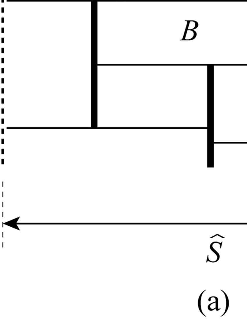
Figure 1.1. (a) The union of vertical segments is $\mathcal{A}$. (b) The shaded region represents $W$.

For a vertical annulus $A=l\times J$, $U=\mathrm{Int}(L\times J)$ is called a vertical solid torus (for short v.s.-torus) with the geodesic core $A$, where $L$ be an equidistant regular neighborhood of $l$ in $S$. Then $L\times J$ is the closure $\overline{U}$ of $U$ in $S\times\widehat{\mathbf{R}}$. We set $\partial\overline{U}=\partial U$ for simplicity. A simple loop in $\partial U$ is a longitude of $U$ if it is isotopic in $\partial U$ to a component of $\partial A$. A meridian of $\partial U$ is a simple loop in $\partial U$ which is non-contractible in $\partial U$ but contractible in $\overline{U}$. For any annulus union $\mathcal{A}$ in $\widehat{S}\times\widehat{\mathbf{R}}$, there exists a disjoint union $\mathcal{V}$ of v.s.-tori the union of whose geodesic cores is equal to $\mathcal{A}$. Then $\mathcal{V}$ is called a v.s.-torus union with the geodesic core $\mathcal{A}$. In general, the union $\mathcal{V}^{\bullet}$ of the closures of components of $\mathcal{V}$ is not equal to the closure $\overline{\mathcal{V}}$ of $\mathcal{V}$ in $S\times\widehat{\mathbf{R}}$. A horizontal surface of $(S\times\widehat{\mathbf{R}},\mathcal{V})$ is a compact connected surface $F$ in $S\times\{a\}$ for some $a\in\widehat{\mathbf{R}}$ with $\mathrm{Int}F\cap\mathcal{V}^{\bullet}=\emptyset$ and $\partial F\subset\mathcal{V}^{\bullet}$. The horizontal surface is critical if it is contained in a critical horizontal surface of $(\widehat{S}\times\mathbf{R},\mathcal{A})$. For any $B\in\mathcal{B}$, the closure $\mathbf{B}$ of $B\setminus\mathcal{V}^{\bullet}$ in $S\times\widehat{\mathbf{R}}$ is a brick of $(S\times\widehat{\mathbf{R}},\mathcal{V})$. Note that $\mathbf{B}$ is a compact subset of $S\times\widehat{\mathbf{R}}$. The brick decomposition $\boldsymbol{\mathcal{B}}$ of $(S\times\widehat{\mathbf{R}},\mathcal{V})$ is the set of bricks of $(S\times\widehat{\mathbf{R}},\mathcal{V})$. Then the union $W=\bigcup\boldsymbol{\mathcal{B}}$ satisfies

$$S\times\mathbf{R}\setminus\mathcal{V}\subset W\subset S\times\widehat{\mathbf{R}}\setminus\mathcal{V},$$

see Fig. 1.1 (b). When $\mathbf{B}\in\boldsymbol{\mathcal{B}}$ is contained in $B\in\mathcal{B}$, set $\partial_{\mathrm{hz}}\mathbf{B}=\partial_{\mathrm{hz}}B\cap\mathbf{B}$, $\partial_{\pm}\mathbf{B}=\partial_{\pm}B\cap\mathbf{B}$ and let $\partial_{\mathrm{vt}}\mathbf{B}$ be the closure of $\partial\mathbf{B}\setminus\partial_{\mathrm{hz}}\mathbf{B}$ in $\partial\mathbf{B}$.

1.4. Geometric limits and bounded geometry

We say that a sequence $\{(N_{n},x_{n})\}$ of hyperbolic 3-manifolds with base points converges geometrically to a hyperbolic 3-manifold $(N_{\infty},x_{\infty})$ with base point if there exist monotone decreasing and increasing sequences $\{K_{n}\}$, $\{R_{n}\}$ with $\lim_{n\rightarrow\infty}K_{n}=1$, $\lim_{n\rightarrow\infty}R_{n}=\infty$ and $K_{n}$-bi-Lipschitz maps

$$g_{n}:\mathcal{N}_{R_{n}}(x_{n},N_{n})\longrightarrow\mathcal{N}_{R_{n}}(x_{\infty},N_{\infty}),$$

where $\mathcal{N}_{R}(x,N)$ denotes the closed $R$-neighborhood of $x$ in $N$. It is well known that, if $\inf\{\mathrm{inj}_{N_{n}}(x_{n})\}>0$, then $\{(N_{n},x_{n})\}$ has a geometrically convergent subsequence, for example see [JM, BP]. If we take a Margulis constant $\varepsilon>0$ sufficiently small, then one can choose the bi-Lipschitz maps so that $g_{n}(\mathcal{N}_{R_{n}}(x_{n},N_{n})_{[\varepsilon,\infty)})=\mathcal{N}_{R_{n}}(x_{\infty},N_{\infty})_{[\varepsilon,\infty)}$, where $\mathcal{N}_{R}(x,N)_{[\varepsilon,\infty)}=\mathcal{N}_{R}(x,N)\cap N_{[\varepsilon,\infty)}$.

In general, the topological type of the limit manifold $N_{\infty}$ is very complicated, for example see [OS]. In spite of the fact, by observing situations in geometric limits, we often know the existence of useful uniform constants. We will give here typical examples.

Example 1.3.

Let $F$ be a connected compact surface and $N$ a hyperbolic 3-manifolds as in Subsection 1.2. Suppose that $\mathrm{Teich}_{\varepsilon}(F)$ is the Teichmüller space such that, for any $\sigma\in\mathrm{Teich}(F)$, $F(\sigma)$ represents a hyperbolic structure on $F$ each boundary component of which is a geodesic loop of length $\varepsilon$. Let $f_{i}:F(\sigma_{i})\longrightarrow N_{[\varepsilon,\infty)}$ $(i=0,1)$ be $K$-Lipschitz maps properly homotopic to each other in $N_{[\varepsilon,\infty)}$, where $K\geq 1$ and $\sigma_{i}\in\mathrm{Teich}_{\varepsilon}(F)$ $(i=0,1)$. For the homotopy $H:F\times[0,1]\longrightarrow N_{[\varepsilon,\infty)}$ and a point $x\in F$, the image $H(\{x\}\times[0,1])$ is said to be a homotopy arc connecting $f_{0}(F)$ and $f_{1}(F)$. Here we will show by invoking a geometric limit argument that there exists a constant $d_{0}>0$ depending only on $\varepsilon,d_{1},K$ and the topological type of $S$ such that, if there exists a homotopy arc connecting $f_{0}(F)$ with $f_{1}(F)$ of length at most $d_{1}$, then $\mathrm{dist}_{\mathrm{Teich}_{\varepsilon}(F)}(\sigma_{0},\sigma_{1})<d_{0}$.

Suppose contrarily that there would exist a sequence of pairs of homotopy equivalence $K$-Lipschitz maps $f_{i,n}:F(\sigma_{i,n})\longrightarrow N_{n[\varepsilon,\infty)}$ with homotopy arcs $\alpha_{n}$ connecting $f_{0,n}(F)$ with $f_{1,n}(F)$ of length $\leq d_{1}$ and $\mathrm{dist}_{\mathrm{Teich}_{\varepsilon}(F)}(\sigma_{0,n},\sigma_{1,n})\geq n$, where $N_{n}$ are hyperbolic 3-manifolds as in Subsection 1.2. Since the $\varepsilon/K$-thin part of $F(\sigma_{i,n})$ is empty, there exists a $K^{\prime}$-bi-Lipschitz map $\gamma_{i,n}:F(\sigma_{0})\longrightarrow F(\sigma_{i,n})$ for some fixed $\sigma_{0}\in\mathrm{Teich}_{\varepsilon}(F)$, where $K^{\prime}$ is a constant depending only on $\varepsilon$, $K$ and $S$. We note that $\gamma_{i,n}$ does not necessarily preserve the marking on $F$. Let $Q_{n}$ be the union of bounded components of $N_{n[\varepsilon,\infty)}\setminus f_{0,n}(F)\cup f_{1,n}(F)$ and $R_{n}$ a small regular neighborhood of $f_{0,n}(F)\cup f_{1,n}(F)$ in $N_{n[\varepsilon,\infty)}$. Then $J_{n}=R_{n}\cup Q_{n}$ is a compact connected subset of $N_{n[\varepsilon,\infty)}$. By [FHS], we know that $f_{0,n}$ is properly homotopic to $f_{1,n}$ in $J_{n}$. If we take a base point $x_{n}$ of $N_{n}$ in $J_{n}$, then $\{(N_{n},x_{n})\}$ has a subsequence, still denoted by $\{N_{n}\}$, converges geometrically to a hyperbolic 3-manifold $(N_{\infty},x_{\infty})$. Thus we have $K_{n}$-bi-Lipschitz maps $g_{n}:\mathcal{N}_{R_{n}}(x_{n},N_{n})\longrightarrow\mathcal{N}_{R_{n}}(x_{\infty},N_{\infty})$ as above.

For any point $y\in J_{n}$ with $\mathrm{dist}_{N_{n}[\varepsilon,\infty)}(y,f_{0,n}(F)\cup f_{1,n}(F))>1$, we have a pleated map $g:\widehat{S}\longrightarrow N_{n}$ such that there exists a component $L$ of $g(\widehat{S})\cap N_{n[\varepsilon,\infty)}$ meeting the $1$-neighborhood of $x$ in $N_{n[\varepsilon,\infty)}$. It is not hard to see that $L$ meets $f_{0,n}(F)\cup\alpha_{n}\cup f_{1,n}(F)$ non-trivially and the diameter of $L$ is bounded by a constant depending only on $\varepsilon$, $S$. Thus the diameter of $J_{n}$ is less than a constant $R>0$ depending only on $\varepsilon,d_{1},K,S$ and hence $J_{n}$ is contained in $\mathcal{N}_{R_{n}}(x_{n},N_{n})_{[\varepsilon,\infty)}$ for all sufficiently large $n$.

By the Ascoli-Arzelà Theorem, if necessarily passing to subsequences, one can show that $\psi_{i,n}=g_{n}\circ f_{i,n}\circ\gamma_{i,n}:F(\sigma_{0})\longrightarrow N_{\infty[\varepsilon,\infty)}$ $(i=0,1)$ converge uniformly to $KK^{\prime}$-Lipschitz maps $\varphi_{i}:F(\sigma_{0})\longrightarrow N_{\infty[\varepsilon,\infty)}$. Since $\psi_{i,n}$ $(i=0,1)$ is properly homotopic to $\varphi_{i}$ for all sufficiently large $n$ and $f_{0,n}\circ\gamma_{0,n}$ is properly homotopic to $f_{1,n}\circ\gamma_{1,n}$ in $J_{n}$ up to marking, there exists a diffeomorphism (hence a $K^{\prime\prime}$-bi-Lipschitz map for some $K^{\prime\prime}\geq 1$) $\alpha:F(\sigma_{0})\longrightarrow F(\sigma_{0})$ such that $\varphi_{0}$ is properly homotopic to $\varphi_{1}\circ\alpha$ in a small compact neighborhood of $g_{n}(J_{n})$ in $N_{\infty[\varepsilon,\infty)}$. This implies that, for any non-contractible simple closed curve $l$ in $F$, $\gamma_{0,n}(l)$ is homotopic to $\gamma_{1,n}\circ\alpha(l)$ in $F$. Thus $\gamma_{1,n}\circ\alpha\circ\gamma_{0,n}^{-1}:F(\sigma_{0,n})\longrightarrow F(\sigma_{1,n})$ is a marking-preserving ${K^{\prime}}^{2}K^{\prime\prime}$-bi-Lipschitz map for all sufficiently large $n$, which contradicts that $\mathrm{dist}_{\mathrm{Teich}_{\varepsilon}(F)}(\sigma_{0,n},\sigma_{1,n})\geq n$. This shows that the existence of our desired uniform constant $d_{0}$.

Example 1.4.

We work in the situation as in the previous example and suppose moreover that there exists a constant $d_{2}>0$ with $\mathrm{dist}_{N_{n[\varepsilon,\infty)}}(f_{0,n}(F),f_{1,n}(F))\geq d_{2}$ for all $n$ and each $f_{i,n}$ is properly homotopic in $N_{n[\varepsilon,\infty)}$ to an embedding. By [FHS], one can suppose that such an embedding is contained in an arbitrarily small regular neighborhood of $f_{i,n}(F)$ in $N_{n[\varepsilon,\infty)}$ and the image of the homotopy is in $J_{n}$ given as above. Then $\varphi_{i}:F\longrightarrow N_{\infty[\varepsilon,\infty)}$ $(i=0,1)$ are also homotopic to embeddings $\varphi_{i}^{\prime}$ contained in an arbitrarily small regular neighborhood of $\varphi_{i}(F)$ in $N_{\infty[\varepsilon,\infty)}$ and the image of the homotopy is in $g_{n}(J_{n})$ for a sufficiently large $n$. By the standard theory of 3-manifold topology (for example see [Wa, He]), the union $\varphi_{0}^{\prime}(F)\cup\varphi_{1}^{\prime}(F)$ bounds a submanifold $B$ of $N_{\infty[\varepsilon,\infty)}$ contained in $g_{n}(J_{n})$ and homeomorphic to $F\times[0,1]$. Then, for all sufficiently large $n$, $B_{n}=g_{n}^{-1}(B)$ is the submanifold of $N_{n[\varepsilon,\infty)}$ such that $\mathrm{Fr}(B_{n})$ consists of two components $F_{i,n}$ $(i=0,1)$ properly homotopic to $f_{i,n}(F)$ in $J_{n}$. Since the composition $g_{m}^{-1}\circ g_{n}|B_{n}$ defines a marking-preserving $K_{m}K_{n}$-bi-Lipschitz map from $B_{n}$ to $B_{m}$ and since $\lim_{m,n\rightarrow\infty}K_{m}K_{n}=1$, we know that $B_{n}$’s have the geometry uniformly bounded by constants depending only on $\varepsilon,d_{1},d_{2}$ and the topological type of $S$.

Remark 1.5.

Deform the metric on $N_{n[\varepsilon,\infty)}$ in a small collar neighborhood of $\partial N_{n[\varepsilon,\infty)}$ so that $\partial N_{n[\varepsilon,\infty)}$ is locally convex but the sectional curvature of $N_{n[\varepsilon,\infty)}$ is still pinched. We here consider the case that $f_{i,n}:F(\sigma_{i})\longrightarrow N_{n[\varepsilon,\infty)}$ $(i=0,1)$ are embeddings which have the least area among all maps homotopic to $f_{i,n}$ without moving $f_{i,n}|_{\partial F(\sigma_{i})}$ and such that $\mathrm{Area}(F(\sigma_{i}))$ is bounded by a constant independent of $n$. Then the limits $\varphi_{i}:F\longrightarrow N_{\infty[\varepsilon,\infty)}$ are least area maps (see [HS, Lemma 3.3]), and hence by [FHS] they are also embeddings. Thus, in Example 1.4, one can suppose that $\varphi_{i}^{\prime}=\varphi_{i}$ and hence the frontier of the manifold $B$ is $\varphi_{0}(F)\cup\varphi_{1}(F)$.

2. Three-dimensional approach to hierarchies

We study hierarchies in the curve graph $\mathcal{C}(S)$ introduced by [MM2]. We realize them as families of annulus unions in $\widehat{S}\times\widehat{\mathbf{R}}$, the original idea of which is due to [Bow3, Section 4].

2.1. Hierarchies

Let $\boldsymbol{p}_{\nu}=(\boldsymbol{p}_{-},\boldsymbol{p}_{+})$ be the pair of generalized pants decompositions on $\widehat{S}$ given in Subsection 1.2. We denote by $\mathcal{B}_{0}$ and $\widehat{\mathcal{B}}_{0}$ the single element set $\{\widehat{S}\times\widehat{\mathbf{R}}\}$. Consider a tight geodesic $g_{0}=\{v_{i}\}_{i\in I}$ with $\boldsymbol{i}(g_{0})=\boldsymbol{p}_{-}$ and $\boldsymbol{t}(g_{0})=\boldsymbol{p}_{+}$, where $I$ is an interval in $\mathbf{Z}$. In this section, we always assume that, for any disjoint union $v$ of simple geodesic loop $l_{1},\dots,l_{k}$ in $\widehat{S}$, $A(v)$ represents a union of vertical annuli $A_{i}$ $(i=1,\dots,k)$ in $\widehat{S}\times\widehat{\mathbf{R}}$ with $A_{i}^{S}=l_{i}$ and $A_{i}^{\mathbf{R}}=A_{j}^{\mathbf{R}}$ for all $i,j\in\{1,\dots,k\}$. Thus $A(v)$ is determined uniquely from $v$ and $A(v)^{\mathbf{R}}$.

Suppose that $\xi(S)>1$ and $\boldsymbol{p}_{-}$, $\boldsymbol{p}_{+}$ are in $\widehat{S}\times\{-\infty\}$ and $\widehat{S}\times\{\infty\}$ respectively. When $i\in I$ is not either $\inf(I)$ or $\sup(I)$, $A(v_{i})$ is defined to be the union of vertical annuli in $\widehat{S}\times\mathbf{R}$ with $A(v_{i})^{\mathbf{R}}=[i,i+1]$. When $i=\sup{I}<\infty$ (resp. $i=\inf{I}>-\infty$), let $A(v_{i})^{\mathbf{R}}=[i,\infty]$ (resp. $A(v_{i})^{\mathbf{R}}=[-\infty,i+1]$). We say that $\mathcal{A}(g_{0})=\bigcup_{i=0}^{n}A(v_{i})$ is the annulus union determined from the tight geodesic $g_{0}$. Let $\mathcal{B}_{1}$ be the brick decomposition of $(\widehat{S}\times\widehat{\mathbf{R}},\mathcal{A}(g_{0}))$. An element $B\in\mathcal{B}_{1}$ is said to be connectable if both $\partial_{\pm}B\cap\mathcal{A}_{0}$ are not empty, where $\mathcal{A}_{0}=\mathcal{A}(g_{0})\cup\boldsymbol{p}_{-}\cup\boldsymbol{p}_{+}$. Let $\widehat{\mathcal{B}}_{1}$ be the subset of $\mathcal{B}_{1}$ consisting of connectable bricks $B$ with $\xi(B)>1$, where $\xi(B)=\xi(B^{S})$. If $\xi_{\mathrm{max}}(\mathcal{B}_{1})=\max\{\xi(B);B\in\mathcal{B}_{1}\}>1$, then any $B\in\mathcal{B}_{1}$ with $\xi(B)=\xi_{\mathrm{max}}(\mathcal{B}_{1})$ is an element of $\widehat{B}_{1}$.

For any $B\in\widehat{\mathcal{B}}_{1}$, consider a tight geodesic $g_{B}$ in $B^{S}$ with $\boldsymbol{i}(g_{B})=(\partial_{-}B\cap\mathcal{A}_{0})^{S}$ and $\boldsymbol{t}(g_{B})=(\partial_{+}B\cap\mathcal{A}_{0})^{S}$. One can define the annulus union $\mathcal{A}_{B}$ of vertical annuli in $B$ determined from $g_{B}$ as above. In particular, $\mathcal{A}_{B}$ consists of vertical annuli with the same width unless the length of $g_{B}$ is finite and $B^{\mathbf{R}}\cap\{-\infty,\infty\}\neq\emptyset$. Note that $\mathcal{A}_{B}$ is a single annulus when the initial vertex of $g_{B}$ is equal to the terminal vertex of $g_{B}$. Set $\mathcal{A}_{1}=\mathcal{A}_{0}\cup\bigl{(}\bigcup_{B\in\widehat{\mathcal{B}}_{1}}\mathcal{A}_{B}\bigr{)}$, $\boldsymbol{i}(\mathcal{A}_{B})=\partial_{-}B\cap\mathcal{A}_{0}$ and $\boldsymbol{t}(\mathcal{A}_{B})=\partial_{+}B\cap\mathcal{A}_{0}$.

Repeating the same argument at most $\xi(S)-1$ times, say $k$ times, one can show that each element $B$ of the set $\mathcal{B}_{k}$ of bricks of $(\widehat{S}\times\widehat{\mathbf{R}},\mathcal{A}_{k-1})$ has $\xi(B)=1$. Since $\xi_{\mathrm{max}}(\mathcal{B}_{k})=1$, each $B\in\mathcal{B}_{k}$ is connectable. We set then $\mathcal{B}_{k}=\widehat{\mathcal{B}}_{k}$. Let $g_{B}=\{w_{i}\}$ be a tight geodesic in $B^{S}$ with $\boldsymbol{i}(g_{B})=(\partial_{-}B\cap\mathcal{A}_{k-1})^{S}$ and $\boldsymbol{t}(g_{B})=(\partial_{+}B\cap\mathcal{A}_{k-1})^{S}$. Since $w_{i}\cap w_{i+1}\neq\emptyset$, we need to add a buffer brick between $A(w_{i})$ and $A(w_{i+1})$ to make them mutually disjoint. Suppose that $B^{\mathbf{R}}=[a,b]$. If $a\neq-\infty$ and $b\neq\infty$ and $g_{B}=(w_{0},w_{1},\dots,w_{m})$, then $A(w_{i})^{\mathbf{R}}=[a+2i\tau,a+(2i+1)\tau]$ for $i=0,1,\dots,m$, where $\tau=(b-a)/(2m+1)$. Note that $B^{S}\times[a+(2i+1)\tau,a+(2i+2)\tau]$ is the buffer brick between $A(w_{i})$ and $A(w_{i+1})$. If $a\neq-\infty$ and $b=\infty$ and $g_{B}=(w_{0},w_{1},\dots,w_{m})$, then $A(w_{i})^{\mathbf{R}}=[a+2i,a+2i+1]$ for $i=0,1,\dots,m-1$ and $A(w_{m})^{\mathbf{R}}=[a+2m,\infty]$. If $a\neq-\infty$ and $b=\infty$ and $g_{B}=(w_{0},w_{1},\dots)$, then $A(w_{i})^{\mathbf{R}}=[a+2i,a+2i+1]$ for all $i$. In the case that $a=-\infty$, $A(w_{i})$ for $w_{i}\in g_{B}$ is defined similarly. As above, let $\mathcal{A}_{B}=\bigcup_{w_{i}\in g_{B}}A(w_{i})$, $\boldsymbol{i}(\mathcal{A}_{B})=\partial_{-}B\cap\mathcal{A}_{k-1}$ and $\boldsymbol{t}(\mathcal{A}_{B})=\partial_{+}B\cap\mathcal{A}_{k-1}$.

When $B\in\widehat{\mathcal{B}}_{j}$, we say that the level of $B$ is $j$ and denote it by $\mathrm{level}(B)$. The set $H_{\nu}$ of all tight geodesics appeared in this construction is called a hierarchy associated to the pair $\boldsymbol{p}_{\nu}=(\boldsymbol{p}_{-},\boldsymbol{p}_{+})$ of generalized pants decompositions and

$$\mathcal{A}_{H_{\nu}}=\mathcal{A}_{k-1}\cup\bigl{(}\bigcup_{B\in\mathcal{B}_{k}}\mathcal{A}_{B}\bigr{)}$$

is the annulus union determined by $H_{\nu}$. Note that the set $H_{\nu}$ is not necessarily defined from $\boldsymbol{p}_{\nu}$ uniquely.

For any $B\in\widehat{B}_{j}$, a maximal brick $C$ in $B$ with $\mathrm{Int}C\cap\mathcal{A}_{B}=\emptyset$ and $\partial_{\mathrm{vt}}C\subset\mathcal{A}_{B}$ is called a subbrick of $B$. From our construction, for any $B\in\widehat{\mathcal{B}}_{j}$ with $0<j\leq k$, there exists either a brick $B^{\prime}\in\mathcal{B}_{j-1}$ with $\partial_{+}B^{\prime}=\partial_{+}B$ or a subbrick $C$ of some element of $\widehat{\mathcal{B}}_{j-1}$ with $\partial_{+}C=\partial_{+}B$. In the former case, $B^{\prime}$ is not in $\widehat{\mathcal{B}}_{j-1}$, otherwise $B$ would be split by $\mathcal{A}_{B^{\prime}}\subset\mathcal{A}_{j-1}$. Repeating the same argument, we have eventually a brick $B_{0}\in\widehat{\mathcal{B}}_{j_{0}}$ for some $j_{0}<j$ which contains a subbrick $C$ with $\partial_{+}C=\partial_{+}B$. Then we say that $B$ is directly forward subordinate to $B_{0}$ and denote it by $B\ {\searrow}\!\!{}^{d}\ B_{0}$. The directly backward subordinate $B_{0}\ {}^{d}\!\!{\swarrow}\ B$ is defined similarly, see Fig. 2.1. It is possible that $B$ is directly forward and backward to the same brick $B_{0}$, i.e. $B_{0}\ {}^{d}\!\!{\swarrow}\ B\ {\searrow}\!\!{}^{d}\ B_{0}$.

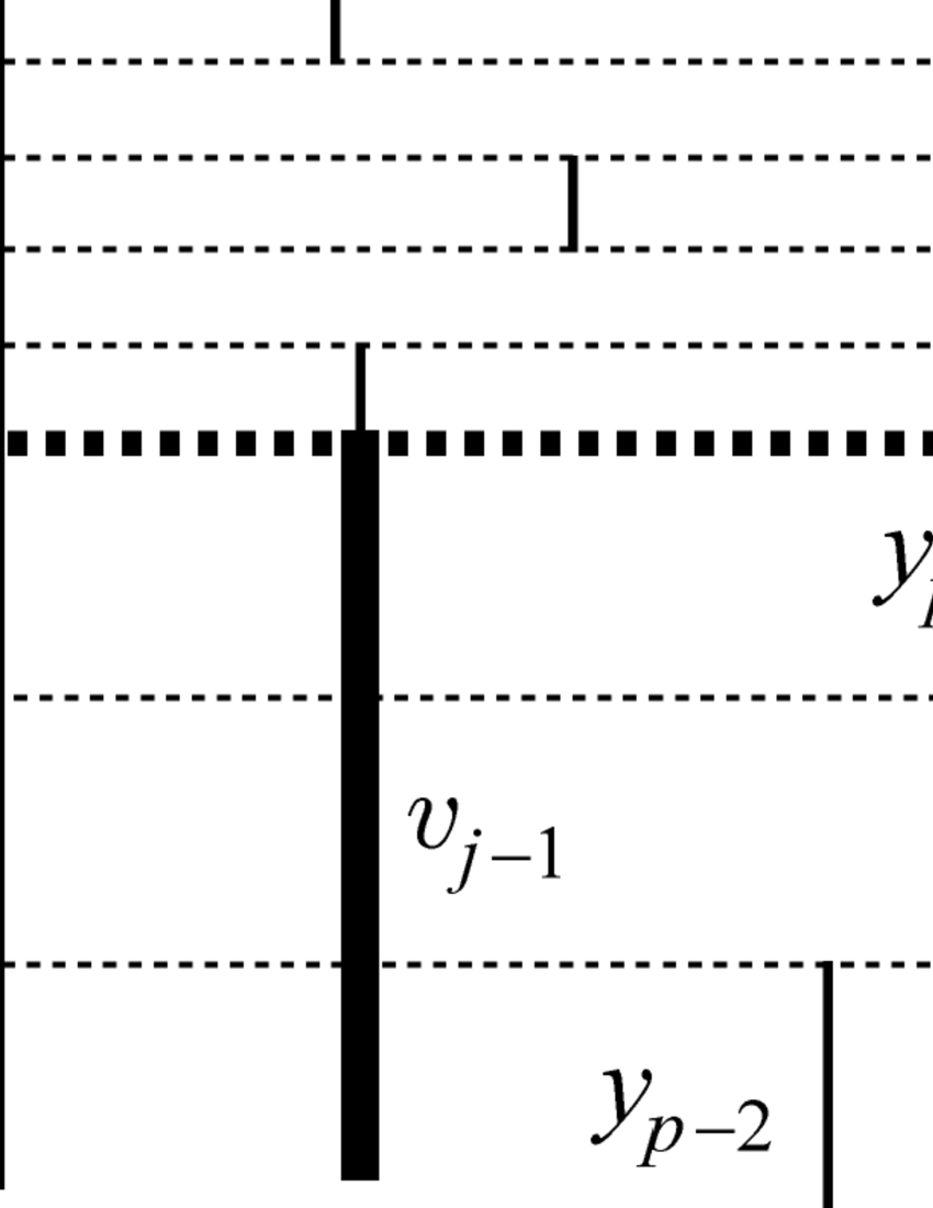
Figure 2.1. Let $g_{0}=(\dots,v_{j-1},v_{j},v_{j+1},\dots)$ be a tight geodesic in the closed surface $S$ of genus $2$. Let $B_{a}\in\widehat{\mathcal{B}}_{1}$ $(a=j\pm 1)$ be the element with $\partial_{\mathrm{vt}}B_{a}=A(v_{a})$. Let $B_{j,1},B_{j,2}$ be the elements of $\mathcal{B}_{1}$ whose vertical boundaries are $A(v_{j})$ and such that $B_{j,1}$ is connectable but $B_{j,2}$ is not. $(v_{j}=x_{0},x_{1},x_{2},\dots)$ is a tight geodesic in $B_{j+1}^{S}$ and $(\dots,y_{p-1},y_{p-1},y_{p}=v_{j})$ is a tight geodesic in $B_{j-1}^{S}$. The shaded region represents an element $B=C_{j-1}\cup B_{j,2}\cup C_{j+1}$ of $\widehat{\mathcal{B}}_{2}$ with $B_{j-1}\ {}^{d}\!\!{\swarrow}\ B\ {\searrow}\!\!{}^{d}\ B_{j+1}$. In fact, we have $\partial_{+}B=\partial_{+}C_{j+1}$ and $\partial_{-}B=\partial_{-}C_{j-1}$, where $C_{a}$ $(a=j\pm 1)$ is the subbrick of $B_{a}$ as illustrated in the figure.

Since only horizontal surfaces of $(\widehat{S}\times\widehat{\mathbf{R}},\mathcal{A}_{i})$ contained in $\mathrm{Int}B$ for some $B\in\widehat{\mathcal{B}}_{i+1}$ are split by $\mathcal{A}_{i+1}$, any critical horizontal surface of $(\widehat{S}\times\widehat{\mathbf{R}},\mathcal{A}_{i})$ is still a (possibly non-critical) horizontal surface of $(\widehat{S}\times\widehat{\mathbf{R}},\mathcal{A}_{i+1})$. The relation $B\ {\searrow}\!\!{}^{d}\ B_{0}$ for $B\in\widehat{\mathcal{B}}_{j}$ and $B_{0}\in\widehat{\mathcal{B}}_{j_{0}}$ implies that, for any $i$ with $j_{0}<i\leq j$, $\partial_{+}B$ is the positive front of some element $B_{i}$ of $\mathcal{B}_{i}$. Since $G=\partial_{+}B\setminus\mathcal{A}_{j_{0}}$ is a union of critical horizontal surfaces of $(\widehat{S}\times\widehat{\mathbf{R}},\mathcal{A}_{j_{0}})$, each component $F$ of $G$ is a horizontal surface of $(\widehat{S}\times\widehat{\mathbf{R}},\mathcal{A}_{j_{0}+1})$. Since moreover $F\subset\partial_{+}B_{j_{0}+2}$, $F$ is critical with respect to $\mathcal{A}_{j_{0}+1}$. Repeating the same argument, one can show that $F$ is a critical horizontal surface of $(\widehat{S}\times\widehat{\mathbf{R}},\mathcal{A}_{j-1})$. It follows that $G=\partial_{+}B\setminus\mathcal{A}_{j-1}=\partial_{+}B\setminus\boldsymbol{t}(\mathcal{A}_{B})$ and hence $\boldsymbol{t}(\mathcal{A}_{B})=\partial_{+}B\cap\mathcal{A}_{j_{0}}$.

2.2. Single brick occupation

Let $\mathcal{A}_{0},\dots,\mathcal{A}_{k-1},\mathcal{A}_{H_{\nu}}$ be the annulus unions and $\mathcal{B}_{0},\dots,\mathcal{B}_{k}$ the brick decompositions given in Subsection 2.1.

Lemma 2.1.

Any two components of $\mathcal{A}_{H_{\nu}}$ are not parallel in $S\times\mathbf{R}$.

Proof.

Suppose that $\mathcal{A}_{H_{\nu}}$ contains distinct mutually parallel components $A,A^{\prime}$. When more than one elements are parallel to $A$, we may assume that $A^{\prime}$ is closest to $A$ among them and $\max A^{\mathbf{R}}<\min{A^{\prime}}^{\mathbf{R}}$. Let $B$ (resp. $B^{\prime}$) be the element of $\widehat{\mathcal{B}}_{k}$ with $\partial_{+}A\subset\mathrm{Int}B$ (resp. $\partial_{-}A^{\prime}\subset\mathrm{Int}B^{\prime}$). Since any two components of $\mathcal{A}_{B}$ are not mutually parallel, $\mathrm{Int}B\cap\mathrm{Int}B^{\prime}$ is empty. Consider a pair of two directly subordinate sequences

(2.1) $$B_{0}\ {\searrow}\!\!{}^{d}\ B_{1}\ {\searrow}\!\!{}^{d}\ \cdots\ {\searrow}\!\!{}^{d}\ B_{m+1},\quad B_{n+1}^{\prime}\ {}^{d}\!\!{\swarrow}\ \cdots\ {}^{d}\!\!{\swarrow}\ B_{1}^{\prime}\ {}^{d}\!\!{\swarrow}\ B^{\prime}_{0}$$

satisfying the following conditions.

1. $B_{0}=B$, $B_{0}^{\prime}=B^{\prime}$, and $\mathrm{Int}B_{i}\cap\mathrm{Int}B_{j}^{\prime}=\emptyset$ for any $0\leq i\leq m$ and $0\leq j\leq n$.

2. The pair (2.1) has the minimum $\max\{\mathrm{level}(B_{m+1}),\mathrm{level}(B_{n+1}^{\prime})\}$ among all pairs of subordinate sequences satisfying the condition (i).

Note that any $B_{i}$ and $B_{j}^{\prime}$ meet the vertical annulus $A_{0}$ with $\partial_{-}A_{0}=\partial_{-}A$ and $\partial_{+}A_{0}=\partial_{+}A^{\prime}$ non-trivially.

First, we will show that $B_{m+1}=B_{n+1}^{\prime}$. For the symmetricity, we may assume that $\mathrm{level}(B_{m+1})\leq\mathrm{level}(B_{n+1}^{\prime})$. Take the entry $B_{i}$ in the the directly forward subordinate sequence with

$$\mathrm{level}(B_{i+1})\leq\mathrm{level}(B_{n+1}^{\prime})<\mathrm{level}(B_{i}).$$

Then there exists an element of $D\in\mathcal{B}_{a}$ with $D\setminus\partial_{-}D\supset\partial_{+}B_{i}$, where $a=\mathrm{level}(B_{n+1}^{\prime})$. Then, in particular, $(\partial_{+}B_{i})^{\mathbf{R}}\leq(\partial_{+}D)^{\mathbf{R}}$. Suppose that $D\neq B_{n+1}^{\prime}$. Since $A$ penetrates both $D$ and $B_{n+1}^{\prime}$, this implies $(\partial_{+}D)^{\mathbf{R}}\leq(\partial_{-}B_{n+1}^{\prime})^{\mathbf{R}}$. If $D\in\widehat{\mathcal{B}}_{a}$, then $B_{i}\ {\searrow}\!\!{}^{d}\ D$ and hence $D=B_{i+1}$. Since then $\mathrm{Int}B_{i+1}\cap\mathrm{Int}B_{n+1}^{\prime}=\emptyset$,

$$B_{0}\ {\searrow}\!\!{}^{d}\ B_{1}\ {\searrow}\!\!{}^{d}\ \cdots\ {\searrow}\!\!{}^{d}\ B_{i+1}\ {\searrow}\!\!{}^{d}\ B_{i+2},\quad B_{n+2}^{\prime}\ {}^{d}\!\!{\swarrow}\ \cdots\ {}^{d}\!\!{\swarrow}\ B_{1}^{\prime}\ {}^{d}\!\!{\swarrow}\ B^{\prime}_{0}$$

is a sequence satisfying the condition (i) and $\max\{\mathrm{level}(B_{i+2}),\mathrm{level}(B_{n+2}^{\prime})\}<a$. If $D\in\mathcal{B}_{a}\setminus\widehat{\mathcal{B}}_{a}$, then $D\neq B_{i+1}$ and hence $\mathrm{level}(B_{i+1})<a$. Thus

$$B_{0}\ {\searrow}\!\!{}^{d}\ B_{1}\ {\searrow}\!\!{}^{d}\ \cdots\ {\searrow}\!\!{}^{d}\ B_{i+1},\quad B_{n+2}^{\prime}\ {}^{d}\!\!{\swarrow}\ \cdots\ {}^{d}\!\!{\swarrow}\ B_{1}^{\prime}\ {}^{d}\!\!{\swarrow}\ B^{\prime}_{0}$$

is a sequence satisfying the condition (i) and $\max\{\mathrm{level}(B_{i+1}),\mathrm{level}(B_{n+2}^{\prime})\}<a$. In either case, this contradicts the minimality condition (ii). It follows that $D=B_{n+1}^{\prime}$. Since this implies $D\in\widehat{\mathcal{B}}_{a}$, $B_{i+1}=D$. Thus we have $i=m$ and $B_{m+1}=B_{n+1}^{\prime}=D$.

For short, set $D^{S}=F$, $A_{0}^{S}=l$, $v=\mathrm{Fr}(\partial_{+}B_{m})$, $w=\mathrm{Fr}(\partial_{-}B_{n}^{\prime})$ and let $t_{m}$ be the component of $\boldsymbol{t}(\mathcal{A}_{B_{m}})$ such that $t_{m}^{S}$ is the terminal vertex of $g_{B_{m}}$. Since $A_{0}\cap(\mathrm{Fr}(\partial_{+}B_{m})\cup\mathrm{Fr}(\partial_{-}B_{n}^{\prime}))=\emptyset$,

$$d_{\mathcal{C}(F)}(v^{S},w^{S})\leq d_{\mathcal{C}(F)}(v^{S},l)+d_{\mathcal{C}(F)}(l,w^{S})=2.$$

Suppose first that $d_{\mathcal{C}(F)}(v^{S},w^{S})=2$ and consider the union $J$ of components of $\mathcal{A}(g_{D})$ with $(\partial_{-}J)^{\mathbf{R}}=v^{\mathbf{R}}$ and $(\partial_{+}J)^{\mathbf{R}}=w^{\mathbf{R}}$, see Fig. 2.2.

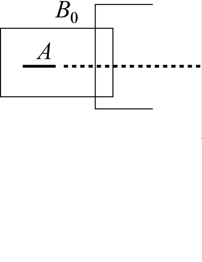
Figure 2.2. The case of $d_{\mathcal{C}(F)}(v^{S},w^{S})=2$.

Since $l\cap(v^{S}\cap w^{S})=\emptyset$, the tightness of $g_{D}$ implies either $l\subset J^{S}$ or $l\cap J^{S}=\emptyset$. However, the former does not occur since $A$ and $A^{\prime}$ are a closest pair. So, we have $A_{0}\cap t_{m}=\emptyset$. When $d_{\mathcal{C}(F)}(v^{S},w^{S})=1$, either $t_{m}\cap\partial_{-}B_{n}^{\prime}=\emptyset$ or $t_{m}\subset w$ holds. This also implies $A_{0}\cap t_{m}=\emptyset$.

Repeating the same argument for $B_{m-1},B_{m-2},\dots,B_{0}=B$, one can show that $A_{0}\cap t_{0}=\emptyset$. This contradicts that the surface $\partial_{+}B$ with $\xi(\partial_{+}B)=1$ can not contain mutually disjoint two curves. Thus any two components of $\mathcal{A}_{H_{\nu}}$ are not parallel to each other. ∎

The following lemma is a geometric version of the fourth assertion of Theorem 4.7 (Structure of Sigma) in [MM2].

Lemma 2.2.

Suppose that $B,B^{\prime}$ are elements of $\widehat{\mathcal{B}}_{a}$ and $\widehat{\mathcal{B}}_{b}$ respectively. If $B^{S}=B^{\prime}{}^{S}$, then $B=B^{\prime}$.

Proof.

We suppose that $B\neq B^{\prime}$ and induce a contradiction.

Since any two elements of $\widehat{B}_{a}$ have mutually disjoint interiors, if $\mathrm{Int}B\cap\mathrm{Int}B^{\prime}\neq\emptyset$, then $a\neq b$, say $a<b$. The assumption $B\in\widehat{\mathcal{B}}_{a}$ implies $\mathcal{A}_{B}\subset\mathcal{A}_{a}\subset\mathcal{A}_{b-1}$. Since $B^{S}=B^{\prime}{}^{S}$, $\mathrm{Int}B\cap\mathrm{Int}B^{\prime}\neq\emptyset$ implies $\mathrm{Int}B^{\prime}\cap\mathcal{A}_{B}\neq\emptyset$. This contradicts the fact that $\mathrm{Int}B^{\prime}\cap\mathcal{A}_{b-1}(\supset\mathrm{Int}B^{\prime}\cap\mathcal{A}_{B})$ is empty. Thus we have $\mathrm{Int}B\cap\mathrm{Int}B^{\prime}=\emptyset$.

Now, we consider a sequence

$$B=B_{0}\ {\searrow}\!\!{}^{d}\ B_{1}\ {\searrow}\!\!{}^{d}\ \cdots\ {\searrow}\!\!{}^{d}\ B_{m+1}=D=B_{n+1}^{\prime}\ {}^{d}\!\!{\swarrow}\ \cdots\ {}^{d}\!\!{\swarrow}\ B_{1}^{\prime}\ {}^{d}\!\!{\swarrow}\ B^{\prime}_{0}=B^{\prime}$$

as in the proof of Lemma 2.1. Let $E$ be the brick in $\widehat{S}\times\widehat{\mathbf{R}}$ with $\partial_{-}E=\partial_{-}B$ and $\partial_{+}E=\partial_{+}B^{\prime}$. We set $E^{S}=H$ and $H_{j}=E\cap\partial_{+}B_{j}$. Since $H\subset\partial_{+}B_{m}^{S}\cap\partial_{-}B_{n-1}^{S}$, the smallest surface $F^{\prime}$ in $F=D^{S}$ with geodesic boundary and containing $F\setminus\mathrm{Int}(\partial_{+}B_{m}^{S}\cap\partial_{-}B_{n-1}^{S})$ is disjoint from $\mathrm{Int}H$. Since $g_{D}$ is a tight geodesic in $F$, the terminal vertex $t_{m}^{S}$ of $g_{B_{m}}$ with $t_{m}\subset\boldsymbol{t}(\mathcal{A}_{B_{m}})$ is contained in $F^{\prime}$ and hence $\mathrm{Int}H_{m}\cap t_{m}=\emptyset$. Repeating the same argument for $B_{m-1},\dots,B_{0}=B$, one can show that $\mathrm{Int}(\partial_{+}B_{0})=\mathrm{Int}H_{0}$ is disjoint from $t_{0}$. This contradicts that $B_{0}$ is a connectable brick with $B_{0}\ {\searrow}\!\!{}^{d}\ B_{1}$. Thus we have $B=B^{\prime}$. ∎

Let $B$ be an element of $\mathcal{B}_{i}$. If $B$ is not connectable, then $\mathrm{Int}B\cap\mathcal{A}_{i}=\emptyset$. Thus there exists a $C\in\mathcal{B}_{i+1}$ with $C\supset B$ and $C^{S}=B^{S}$ (possibly $B=C$). Repeating the same argument if $C$ is not connectable, we have eventually a unique element $B^{\vee}$ of $\widehat{\mathcal{B}}_{j}$ with $j\geq i$, $B^{\vee}\supset B$ and $B^{\vee S}=B^{S}$, which is called the expanding connectable brick of $B$. For example, $C_{j-1}\cup B_{j,2}\cup C_{j+1}\in\widehat{\mathcal{B}}_{2}$ in Fig. 2.1 is the expanding connectable brick of $B_{j,2}\in\mathcal{B}_{1}$.

The following lemma suggests that a large part of any longer brick $Q$ in $\widehat{S}\times\widehat{\mathbf{R}}$ with $\partial_{\mathrm{vt}}Q\subset\mathcal{A}_{H_{\nu}}$ is occupied by a single brick in $\widehat{\mathcal{B}}_{a}$ for some $a$.

Lemma 2.3 (Single brick occupation).

There exists an integer $n_{0}$ depending only on $\xi(S)$ such that, for any brick $Q$ in $\widehat{S}\times\widehat{\mathbf{R}}$ with $\xi(Q)\geq 1$ and $\partial_{\mathrm{vt}}Q\subset\mathcal{A}_{H_{\nu}}$, there is a set $\mathcal{B}_{Q}=\{B_{1},\dots,B_{n}\}$ of bricks in $Q$ with $\partial_{\mathrm{vt}}B_{i}\subset\mathcal{A}_{H_{\nu}}$ and satisfying the following conditions.

1. $n\leq n_{0}$ and $\overline{\bigcup\mathcal{B}_{Q}}=\overline{B}_{1}\cup\cdots\cup\overline{B}_{n}\supset Q$.

2. For at most one of the elements of $\mathcal{B}_{Q}$, say $B_{1}$, there exists a brick $C$ in $\widehat{\mathcal{B}}_{a}$ with $C^{S}=Q^{S}$ and $C\cap Q=B_{1}$ for some $a$. For all other bricks $B_{i}$ of $\mathcal{B}_{Q}$, $\partial_{\mathrm{vt}}B_{i}\cap\mathrm{Int}Q$ is non-empty.

We note that $B_{i}$ are not necessarily elements of $\mathcal{B}_{a}$ $(a=0,\dots,k)$.

Proof.

When $Q^{S}=\widehat{S}$, the pair $C=\widehat{S}\times\widehat{\mathbf{R}}\in\widehat{\mathcal{B}}_{0}$ and $\mathcal{B}_{Q}=\{Q\}$ satisfy the conditions (i) and (ii). So we may assume that $Q^{S}\neq\widehat{S}$ or equivalently $\partial_{\mathrm{vt}}Q\neq\emptyset$. In particular, $\xi(\widehat{S})>1$. Recall that, for each entry $v_{i}$ of the tight geodesic $g_{0}=\{v_{i}\}$ in $\widehat{S}$, $A(v_{i})$ is contained in $\mathcal{A}_{H_{\nu}}$. Since $\partial_{\mathrm{vt}}Q\subset\mathcal{A}_{H_{\nu}}$, $A(v_{i})^{\mathbf{R}}\cap\mathrm{Int}Q^{\mathbf{R}}\neq\emptyset$ means that $d_{\mathcal{C}(\widehat{S})}(w_{i},x)\leq 1$ for any vertices $w_{i}$ of $v_{i}$ and any component $x$ of $\partial_{\mathrm{vt}}Q^{S}$. It follows that $A(v_{i})^{\mathbf{R}}\cap\mathrm{Int}Q^{\mathbf{R}}\neq\emptyset$ for at most three succeeding entries $v_{i}$ of $g_{0}$. Thus the brick decomposition of $(Q,\mathcal{A}_{0}\cap Q)$ consists of at most $-3\chi(Q^{S})$ subbricks $C_{1},\dots,C_{m}$ of $Q$. Let $\mathcal{B}_{Q}^{(0)}$ be the set of $C_{i}$ with $\partial_{\mathrm{vt}}C_{i}\cap\mathrm{Int}Q\neq\emptyset$. For any $C_{i}$ not in $\mathcal{B}_{Q}^{(0)}$, there exists a unique $D_{i}$ of $\mathcal{B}_{1}$ with $D_{i}\cap Q\supset C_{i}$. Let $\mathcal{B}_{Q}^{(1)}$ be the set of $C_{i}$ with $D_{i}^{S}=Q^{S}$.

Suppose that $C_{i}$ is not in $\mathcal{B}_{Q}^{(0)}\cup\mathcal{B}_{Q}^{(1)}$. Then $Q^{S}$ is a proper subsurface of $D_{i}^{S}$ and $\mathrm{Int}D_{i}\cap\partial_{\mathrm{vt}}Q$ is not empty. We repeat the argument as above for $(D_{i}^{\vee},D_{i}^{\vee}\cap Q)$ instead of $(\widehat{S}\times\widehat{\mathbf{R}},Q)$, where $D_{i}^{\vee}$ is the expanding connectable brick of $D_{i}$. Then we have the sets $\mathcal{B}_{D_{i}^{\vee}\cap Q}^{(0)}$ and $\mathcal{B}_{D_{i}^{\vee}\cap Q}^{(1)}$ of bricks in $D_{i}^{\vee}\cap Q$ as above. Since $1<\xi(D_{i}^{\vee})<\xi(\widehat{S})$, this repetition finishes at most $\xi(\widehat{S})-\xi(Q)$ times. Eventually we have at most $(-3\chi(Q^{S}))^{\xi(\widehat{S})-\xi(Q)}$ bricks $B_{j}^{\prime}$ in $Q$ with $\bigcup_{j}\overline{B_{j}^{\prime}}\supset Q$, $\partial_{\mathrm{vt}}B_{j}^{\prime}\subset\mathcal{A}_{H_{\nu}}$ such that either $\partial_{\mathrm{vt}}B_{j}^{\prime}\cap\mathrm{Int}Q\neq\emptyset$ or there exists an element $D_{j}^{\vee}\in\widehat{\mathcal{B}}_{a}$ for some $a$ with $D_{j}^{\vee}\supset B_{j}^{\prime}$ and $D_{j}^{\vee S}=Q^{S}$. By Lemma 2.2, all $D_{j}^{\vee}$ appeared in the latter case are the same brick $C$. The set $\mathcal{B}_{Q}$ consisting of all $B_{j}^{\prime}$ in the former case and $Q\cap C$ (if the latter case occurs) satisfies the conditions (i) and (ii) by setting $n_{0}=(-3\chi(\widehat{S}))^{\xi(\widehat{S})-1}$. ∎

3. The model manifold

We will define the model manifold and a piecewise Riemannian metric on it as in [Mi2, Section 8].

A constant $c$ is said to be uniform if $c$ depends only on the topological type of $S$ and previously determined uniform constants, and independent of the end invariants $\nu=(\nu_{-},\nu_{+})$. Throughout the remainder of this paper, for a given constant $k$, a uniform constant $c(k)$ means that it depends only on previously determined uniform constants and $k$.

3.1. Metric on the brick union

Let $\mathcal{A}=\mathcal{A}_{H_{\nu}}$ be the annulus union associated to $H_{\nu}$ given in Section 2 and $\mathcal{V}$ a v.s.-torus union with the geodesic core $\mathcal{A}$. Let $\boldsymbol{\mathcal{B}}$ be the brick decomposition of $(S\times\widehat{\mathbf{R}},\mathcal{V})$ and let $W=\bigcup\boldsymbol{\mathcal{B}}$. Recall that for any $B\in\boldsymbol{\mathcal{B}}$, $\xi(B)=\xi(B^{S})$ is either zero or one. Suppose that $\Sigma_{0,3}$ is a hyperbolic three-holed sphere such that each component of $\partial\Sigma_{0,3}$ is a geodesic loop of length $\varepsilon_{1}$, where $\varepsilon_{1}$ is the constant given in Subsection 1.2. Let $B_{0,3}$ be the product metric space $\Sigma_{0,3}\times[0,1]$. Let $\Sigma_{0,4}$ be a four-holed sphere which has two essential simple closed curves $l_{0},l_{1}$ with the geometric intersection number $i(l_{0},l_{1})=2$, and let $B_{0,4}=\Sigma_{0,4}\times[0,1]$ topologically. Let $A_{i}$ $(i=0,1)$ be a regular neighborhood of $l_{i}\times\{i\}$ in $\Sigma_{0,4}\times\{i\}$. Suppose that $B_{0,4}$ has a piecewise Riemannian metric such that each component of $\Sigma_{0,4}\times\{i\}\setminus\mathrm{Int}A_{i}$ is isometric to the hyperbolic surface $\Sigma_{0,3}$, each component of $A_{0}\cup A_{1}\cup\partial_{\mathrm{vt}}B$ is isometric to the product annulus $S^{1}(\varepsilon_{1})\times[0,1]$ and $\mathrm{dist}_{B_{0,4}}(\partial_{-}B_{0,4},\partial_{+}B_{0,4})=1$, where $S^{1}(\varepsilon_{1})$ is a round circle in the Euclidean plane of circumference $\varepsilon_{1}$. Let $\Sigma_{1,1}$ be a fixed one-holed torus $\Sigma_{1,1}$ with geodesic boundary of length $\varepsilon_{1}$ and essential simple closed curves $l_{0},l_{1}$ with $i(l_{0},l_{1})=1$. Then a piecewise Riemannian metric on $B_{1,1}=\Sigma_{1,1}\times[0,1]$ is defined similarly. We note that these metrics are independent of $\nu$.

For any element $B\in\boldsymbol{\mathcal{B}}$ of type $(i,j)\in\{(0,3),(0,4),(1,1)\}$, consider a diffeomorphism $h_{B}:B_{i,j}\longrightarrow B$ such that $h_{B}(\partial_{\mathrm{vt}}B_{i,j})=\partial_{\mathrm{vt}}B$ and moreover $h_{B}(A_{\pm})=\partial_{\pm}B\cap\mathcal{U}$ when $\xi(B)=1$, where $A_{-}=A_{0}$ and $A_{+}=A_{1}$. One can choose these homeomorphisms so that, for any $B,B^{\prime}$ in $\boldsymbol{\mathcal{B}}$ with $F=\partial_{+}B\cap\partial_{-}B^{\prime}\neq\emptyset$, $(h_{B}|_{h_{B}^{-1}(F)})\circ(h_{B^{\prime}}|_{F})^{-1}$ is an isometry. Then $W$ has the piecewise Riemannian metric induced from those on $B_{0,3},B_{0,4},B_{1,1}$ via embeddings $h_{B}:B\longrightarrow W$. Since any automorphism $\eta:\Sigma_{0,3}\longrightarrow\Sigma_{0,3}$ is isotopic to a unique isometry, the metric on $W$ is uniquely determined up to ambient isotopy.

3.2. Construction of the model manifold

We extend $W$ to the manifold $M_{\nu}[0]$ with piecewise Riemannian metric as in [Mi2, Subsections 3.4 and 8.3]. For any subset $C$ of $S$, we set $C\times\{\infty\}=C^{\{+\}}$ and $C\times\{-\infty\}=C^{\{-\}}$.

Let $\mathcal{V}_{\mathrm{p.c.}}$ (resp. $\mathcal{V}_{\mathrm{g.f.}}$) be the union of components $U$ of $\mathcal{V}$ such that the closure $\overline{U}$ in $S\times\widehat{\mathbf{R}}$ contains a component of $\boldsymbol{q}_{-}^{\{-\}}\cup\boldsymbol{q}_{+}^{\{+\}}$ (resp. $\boldsymbol{r}_{-}^{\{-\}}\cup\boldsymbol{r}_{+}^{\{+\}}$), where $\boldsymbol{r}_{\pm}=\bigcup_{F_{i}\in\mathcal{GF}_{\pm}}\boldsymbol{r}_{i}$. If we denote the complement $\mathcal{V}\setminus(\mathcal{V}_{\mathrm{p.c.}}\cup\mathcal{V}_{\mathrm{g.f.}})$ by $\mathcal{V}_{\mathrm{int.}}$, then $\mathcal{V}$ is represented by the disjoint union

$$\mathcal{V}=\mathcal{V}_{\mathrm{int.}}\cup\mathcal{V}_{\mathrm{g.f.}}\cup\mathcal{V}_{\mathrm{p.c.}}.$$

For any $F_{i}$ in $\mathcal{GF}_{+}$ (resp. in $\mathcal{GF}_{-}$), we suppose that $F_{i}=F_{i}^{\{+\}}$ (resp. $F_{i}=F_{i}^{\{-\}}$) and denote the closure of $(F_{i}\cap S^{\{\pm\}})\setminus\overline{\mathcal{V}}_{\mathrm{p.c.}}$ in $S^{\{\pm\}}$ by $F_{i}^{\prime}$, see Fig. 3.1 (a). Thus $F_{i}^{\prime}$ is a compact surface obtained from $F_{i}$ by deleting the parabolic cusp components. For the conformal structure $\sigma_{i}\in\mathrm{Teich}(F_{i})$ at infinity given in Subsection 1.2, consider the conformal rescaling $\tau_{i}$ of $\sigma_{i}\in\mathrm{Teich}(F_{i})$ such that $\tau_{i}/\sigma_{i}$ is a continuous map which is equal to $1$ on $F_{i}(\sigma_{i})_{[\varepsilon_{1},\infty)}$ and each component of $F_{i}(\sigma_{i})_{(0,\varepsilon_{1}]}$ is a Euclidean cylinder with respect to the $\tau_{i}$-metric. There exists a piecewise Riemannian metric $\upsilon_{i}$ on $F_{i}^{\prime}$ such that $F_{i}^{\prime}(\upsilon_{i})_{(0,\varepsilon_{1}]}$ is equal to $F_{i}^{\prime}\cap\overline{\mathcal{U}}_{\mathrm{g.f.}}$, each component of $F_{i}^{\prime}(\upsilon_{i})_{(0,\varepsilon_{1}]}$ is isometric to a Euclidean cylinder $S^{1}(\varepsilon_{1})\times[0,n]$ with $n\in\mathbf{N}$, and each component of $F_{i}^{\prime}(\upsilon_{i})\setminus\mathrm{Int}F_{i}^{\prime}(\upsilon_{i})_{(0,\varepsilon_{1}]}$ is isometric to $\Sigma_{0,3}$. It is not hard to choose such a metric $\upsilon_{i}$ so that the identity $F_{i}^{\prime}(\tau_{i})\longrightarrow F_{i}^{\prime}(\upsilon_{i})$ is uniformly bi-Lipschitz. Note that our $\upsilon_{i}$ corresponds to the metric ${\sigma^{m}}^{\prime}$ given in [Mi2, Subsection 8.3]. Endow the union $R_{i}=F_{i}^{\prime}\times[-1,0]\cup\partial F_{i}^{\prime}\times[0,\infty)$ with a piecewise Riemannian metric such that (i) $F_{i}^{\prime}\times\{-1\}$ is equal to $F_{i}^{\prime}(\upsilon_{i})$, (ii) $F_{i}^{\prime}\times\{0\}\cup\partial F_{i}^{\prime}\times[0,\infty)$ is isometric $F_{i}(\tau_{i})$ via an isometry whose restriction on $F_{i}^{\prime}$ is the identity, (iii) $\partial F_{i}^{\prime}\times[-1,0]$ is a Euclidean cylinder of width 1 and (iv) the identity from $F_{i}^{\prime}\times[-1,0]$ to the product metric space $F_{i}^{\prime}(\upsilon_{i})\times[-1,0]$ is uniformly bi-Lipschitz. We call that the metric space $R_{i}$ is a boundary brick associated to $\sigma_{i}\in\mathrm{Teich}(F_{i})$ for $F_{i}\in\mathcal{GF}_{+}$. A boundary brick associated to $\sigma_{j}\in\mathrm{Teich}(F_{j})$ for $F_{j}\in\mathcal{GF}_{-}$ is defined similarly. Then $M_{\nu}[0]$ is the metric space obtained by attaching $R_{i}$ to $W$ for any $F_{i}\in\mathcal{GF}_{a}$ $(a=\pm)$ by the isometry $(\partial_{a}B_{1}\cup\cdots\cup\partial_{a}B_{m})\times\{-1\}\longrightarrow\partial_{a}B_{1}\cup\cdots\cup\partial_{a}B_{m}$ isotopic to the identity, where $B_{1},\dots,B_{m}$ are the elements of $\boldsymbol{\mathcal{B}}$ meeting $F_{i}^{\prime}$ non-trivially, see Fig. 3.1 (b).

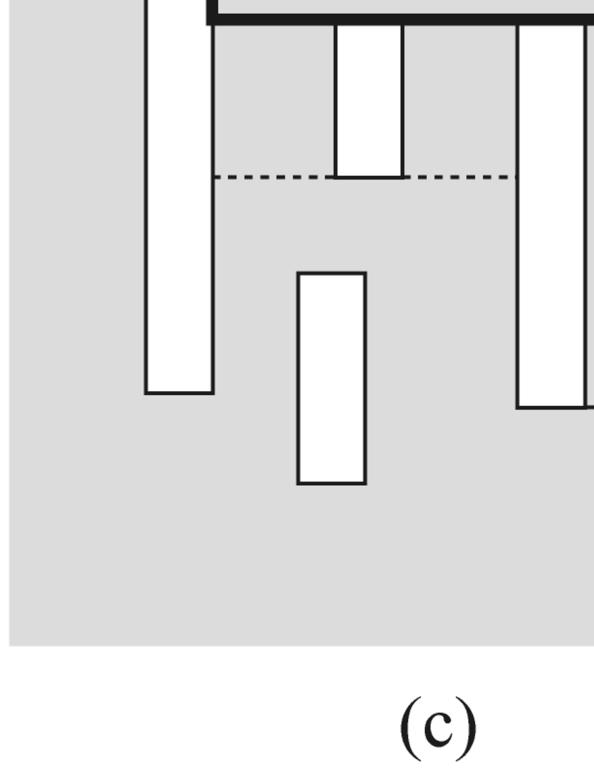
Figure 3.1. (a) Each white rectangle labeled with ‘p.c.’ (resp. ‘g.f.’) represents a component of $\mathcal{V}_{\mathrm{p.c.}}$ (resp. $\mathcal{V}_{\mathrm{g.f.}}$). The shaded regions in (a)–(d) represent $W$, $M_{\nu}[0]$, $M\!E_{\nu}[0]$ and $M_{\nu}$ respectively.

Extend furthermore $M_{\nu}[0]$ by attaching the spaces $F_{i}\times[0,\infty)$ with metric $ds^{2}=\tau_{i}e^{2r}+dr^{2}$ $(r\in[0,\infty))$ for $F_{i}\in\mathcal{GF}_{a}$ $(a=\pm)$ to $M_{\nu}[0]$ by identifying $F_{i}\times\{0\}$ with the ‘outer boundary’ $F_{i}^{\prime}\times\{0\}\cup\partial F_{i}^{\prime}\times[0,\infty)$ of $R_{i}$. We set the extended manifold $M_{\nu}[0]\cup E_{\nu}$ by $M\!E_{\nu}[0]$, where $E_{\nu}=\bigcup_{F_{i}\in\mathcal{GF}_{+}\cup\mathcal{GF}_{-}}F_{i}\times[0,\infty)$. From our construction, we can re-embed $M\!E_{\nu}[0]$ to $S\times\mathbf{R}$ so that there exists a homeomorphism $\eta:\mathcal{V}\longrightarrow\widehat{S}\times\mathbf{R}\setminus M\!E_{\nu}[0]\subset\widehat{S}\times\mathbf{R}$ isotopic to the inclusion $\mathcal{V}\subset\widehat{S}\times\mathbf{R}$ and such that, for any component $U$ of $\mathcal{V}\setminus\mathcal{V}_{\mathrm{g.f.}}$, $\eta|_{U}$ is the identity, see Fig. 3.1 (c). We denote $\eta(\mathcal{V}_{\mathrm{int.}})$ by $\mathcal{U}_{\mathrm{int.}}$, $\eta(\mathcal{V}_{\mathrm{g.f.}})$ by $\mathcal{U}_{\mathrm{g.f.}}$ and $\eta(\mathcal{V}_{\mathrm{p.c.}})\cup\mathcal{U}_{(\widehat{S}\setminus S)}$ by $\mathcal{U}_{\mathrm{p.c.}}$ respectively, where $\mathcal{U}_{(\widehat{S}\setminus S)}=(\widehat{S}\setminus S)\times\mathbf{R}$. Then the complement $\mathcal{U}=\widehat{S}\times\mathbf{R}\setminus M\!E_{\nu}[0]$ is represented by the disjoint union

(3.1) $$\mathcal{U}=\mathcal{U}_{\mathrm{int.}}\cup\mathcal{U}_{\mathrm{g.f.}}\cup\mathcal{U}_{\mathrm{p.c.}}.$$

For any component $U$ of $\mathcal{U}$, the frontier $\partial U$ of $U$ in $\widehat{S}\times\mathbf{R}$ is a torus if $U\subset\mathcal{U}\setminus\mathcal{U}_{\mathrm{p.c.}}$, otherwise $\partial U$ is an open annulus. We set here

$$M_{\nu}=M_{\nu}[0]\cup\mathcal{U}\quad\mbox{and}\quad M\!E_{\nu}=M_{\nu}\cup E_{\nu}\ (=\widehat{S}\times\mathbf{R}).$$

3.3. Meridian coefficients

Let $U=U(v)$ denote the component of $\mathcal{U}\setminus\mathcal{U}_{(\widehat{S}\setminus S)}$ such that $\eta^{-1}(U)\subset\mathcal{V}$ is a v.s.-torus with geodesic core $A(v)$. From our construction of the metric on $M_{\nu}[0]$, any component $\partial U(v)$ is a Euclidean cylinder which has the foliation $\mathcal{F}_{U}=\mathcal{F}_{v}$ consisting of geodesic longitudes of length $\varepsilon_{1}$. For any complex number $z$ with $\mathrm{Im}(z)>0$ and $\eta>0$, we denote the quotient map $\mathbf{C}\longrightarrow\mathbf{C}/\eta(\mathbf{Z}+z\mathbf{Z})$ by $\pi_{z,\eta}$. If $U\subset\mathcal{U}\setminus\mathcal{U}_{\mathrm{p.c.}}$, then we have a unique $\omega\in\mathbf{C}$ with $\mathrm{Im}(\omega)>0$ such that there exists an orientation-preserving isometry from the quotient space $\mathbf{C}/\varepsilon_{1}(\mathbf{Z}+\omega\mathbf{Z})$ to $\partial U$ which maps $\pi_{w,\varepsilon_{1}}(\mathbf{R})$ (resp. $\pi_{w,\varepsilon_{1}}(\omega\mathbf{R})$) to a longitude (resp. a meridian) of $U$. We denote the $\omega$ by $\omega_{M}(U)$ or $\omega_{M}(v)$ and call it the meridian coefficient of $\partial U$. If $U\subset\mathcal{U}_{\mathrm{p.c.}}$, then we define $\omega_{M}(U)=\sqrt{-1}\infty$. Note that $\varepsilon_{1}\mathrm{Im}(\omega_{M}(U))$ is a positive integer whenever $U\subset\mathcal{U}\setminus\mathcal{U}_{\mathrm{p.c.}}$. In fact, the brick decomposition $\boldsymbol{\mathcal{B}}$ induces the decomposition on $\partial U$ consisting of two horizontal annuli with integer width and $\varepsilon_{1}\mathrm{Im}(\omega_{M}(U))-2$ vertical annuli of width one.

For any integer $k>0$, consider the union $\mathcal{U}[k]$ of components $U$ of $\mathcal{U}$ with $|\omega_{M}(U)|\geq k$ and

$$M_{\nu}[k]=M_{\nu}[0]\cup(\mathcal{U}\setminus\mathcal{U}[k])\quad\mbox{and}\quad M\!E_{\nu}[k]=M_{\nu}[k]\cup E_{\nu}.$$

Thus $M_{\nu}=M_{\nu}[k]\cup\mathcal{U}[k]$ and $M\!E_{\nu}=M\!E_{\nu}[k]\cup\mathcal{U}[k]$. We suppose that each component $U$ of $\mathcal{U}\setminus\mathcal{U}[k]$ has a Riemannian metric extending the Euclidean metric on $\partial U$ and isometric to a hyperbolic tube with geodesic core. These metrics define piecewise Riemannian metrics on $M_{\nu}[k]$ and $M\!E_{\nu}[k]$.

4. The Lipschitz model theorem

The Lipschitz Model Theorem given in [Mi2] is a homotopy equivalence map from $M_{\nu}$ to the augmented core $\widehat{C}_{\rho}$ of $N_{\rho}$ such that the restriction to $M_{\nu}[k]$ is a $K$-Lipschitz map for some uniform constant $K$ independent of $\nu,\rho$. The following is the precise statement.

Theorem 4.1 (Lipschitz Model Theorem).

There exists a degree-one, homotopy equivalence map $f:M_{\nu}\longrightarrow\widehat{C}_{\rho}$ with $\pi_{1}(f)=\rho$ and satisfying the following conditions, where $K\geq 1,k\in\mathbf{N}$ are constants independent of $\nu,\rho$.

1. The image $\mathbb{T}[k]=f(\mathcal{U}[k])$ is a union of components of $N_{\rho(0,\varepsilon_{1})}$ with $\mathbb{T}[k]\supset N_{\rho(0,\varepsilon_{2})}$ for some uniform constant $0<\varepsilon_{2}\leq\varepsilon_{1}$ and the restriction $f|_{\mathcal{U}[k]}:\mathcal{U}[k]\longrightarrow\mathbb{T}[k]$ defines a bijection between the components of $\mathcal{U}[k]$ and $\mathbb{T}[k]$.

2. $f(M_{\nu}[k])=\widehat{C}_{\rho}[k]$ and the restriction $f|_{M_{\nu}[k]}:M_{\nu}[k]\longrightarrow\widehat{C}_{\rho}[k]$ is a $K$-Lipschitz map, where $\widehat{C}_{\rho}[k]=\widehat{C}_{\rho}\setminus\mathbb{T}[k]$.

3. The restriction $f|_{\partial M_{\nu}}:\partial M_{\nu}\longrightarrow\partial\widehat{C}_{\rho}$ is a $K$-bi-Lipschitz homeomorphism which can be extended to a $K$-bi-Lipschitz map $f^{\prime}:E_{\nu}\longrightarrow E_{N}$ and moreover to a conformal map from $\partial_{\infty}M\!E_{\nu}$ to $\partial_{\infty}N_{\rho}$. (Moreover, one can construct the map $f$ so that, for any boundary brick $R_{i}$, $f|_{R_{i}}:R_{i}\longrightarrow f(R_{i})$ is $K$-bi-Lipschitz and $f^{-1}(f(R_{i}))=R_{i}$.)

The proof starts with the restriction $f_{0}:M_{\nu}\longrightarrow N_{\rho}$ of a marking-preserving homeomorphism $S\times\mathbf{R}\longrightarrow N_{\rho}$. Minsky’s proof needs the following two lemmas which correspond to Lemmas 7.9 and 10.1 in [Mi2] respectively.

Lemma 4.2 (Length Upper Bounds).

There exists a uniform constant $d_{0}$ such that, for any vertex $v$ appeared in $H_{\nu}$, $l_{\rho}(v)\leq d_{0}$.

Recall that $H_{\nu}$ is the hierarchy defined in Section 2. For any curve $c$ in $M_{\nu}$, $l_{\rho}(c)$ denotes the length of the geodesic in $N_{\rho}$ freely homotopic to $f_{0}(c)$ if any and otherwise $l_{\rho}(c)=0$. We also define $l_{\rho}(v)=l_{\rho}(c)$ for a curve $v$ in $S$ with $v=c^{S}$. As was stated in Introduction, an alternative proof of Lemma 4.2 is given by [Bow2], see also [So] where this lemma is proved by full geometric limit arguments along ideas in [Bow2].

The other key lemma for the Lipschitz Model Theorem is replaced by the following lemma. We will give a shorter proof of it.

Lemma 4.3.

Suppose that $\varepsilon$ is any positive number and there exists a constant $L>0$ with $l_{\rho}(c)\leq L\mathrm{length}_{M_{\nu}[0]}(c)$ for any rectifiable curve $c$ in $M_{\nu}[0]$. Then, there exists a constant $d_{1}$ depending only on $\varepsilon,\varepsilon_{1},L$ such that, for any component $U(v)$ of $\mathcal{U}$ with $|\omega_{M}(v)|>d_{1}$, $l_{\rho}(v)\leq\varepsilon$.

Proof.

Let $\lambda$ be the geodesic loop in $N_{\rho}$ freely homotopic to $f_{0}(v)$. Suppose that $l_{\rho}(v)>\varepsilon$. If $\varepsilon_{1}\mathrm{Im}(\omega_{M}(v))\geq n$, then there exist at least $n$ mutually non-homotopic pleated maps $p_{j}:F(\sigma_{j})\longrightarrow N_{\rho}$ such that each $p_{j}(\partial F)$ contains $\lambda$ , where $F$ is a compact 3-holed sphere. Since $l_{\rho}(v)=\mathrm{length}_{N_{\rho}}(\lambda)>\varepsilon$, all $p_{j}(F(\sigma_{j})_{[\varepsilon,\infty)})$ are contained in a uniformly bounded neighborhood of $\lambda$ in $N_{\rho[\varepsilon,\infty)}$. From this boundedness, we know that $\mathrm{Im}(\omega_{M}(v))$ is bounded by a constant $d$ depending only on $\varepsilon$ and $\varepsilon_{1}$.

Set $U(v)=U$ and let $m$ be the shortest geodesic in $\partial U$ among all geodesics meeting a leaf $l$ of the foliation $\mathcal{F}_{v}$ transversely in a single point. The length of $m$ is at most $(d+1)\varepsilon_{1}$. If $m$ is a meridian of $U$, then $|\omega_{M}(v)|=\mathrm{length}_{\partial U}(m)/\varepsilon_{1}\leq d+1$. Otherwise, $f_{0}|_{m}$ is homotopic to a cyclic covering $\eta:m\longrightarrow\lambda$ whose degree is at most $L(d+1)\varepsilon_{1}/\varepsilon$. This means that the geometric intersection number $\alpha$ of $m$ with a meridian $m_{0}$ of $U$ is at most $L(d+1)\varepsilon_{1}/\varepsilon$. Under a suitable choice of the orientations of $m$ and $l$, the homology class $[m_{0}]\in H_{1}(\partial U,\mathbf{Z})$ is represented by $[m]+\alpha[l]$ and hence

$$|\omega_{M}(v)| =\frac{1}{\varepsilon_{1}}\mathrm{length}_{\partial U}(m_{0})\leq\frac{1}{\varepsilon_{1}}(\mathrm{length}_{\partial U}(m)+\alpha\mathrm{length}_{\partial U}(l))$$

$$\leq(d+1)\Bigl{(}1+\frac{L\varepsilon_{1}}{\varepsilon}\Bigr{)}=:d_{1}.$$

This completes the proof. ∎

4.1. Minsky’s construction

Here we will review briefly how Minsky constructs the Lipschitz map.

Recall that, for each element $B$ of the brick decomposition $\boldsymbol{\mathcal{B}}$ of $(S\times\widehat{\mathbf{R}},\mathcal{V})$ defined in Subsection 3.1, either $\xi(B)=0$ or 1 holds. Let $\boldsymbol{\mathcal{B}}_{\partial}$ be the set of boundary bricks associated to elements of $\mathcal{GF}_{+}\cup\mathcal{GF}_{-}$. In Subsection 3.2, we re-embedded $M_{\nu}[0]=\bigcup(\boldsymbol{\mathcal{B}}\cup\boldsymbol{\mathcal{B}}_{\partial})$ into $S\times\mathbf{R}$ so that $\mathcal{V}$ is identified with $\mathcal{U}\setminus\mathcal{U}_{(\widehat{S}\setminus S)}$, see Fig. 3.1. For any element $B=F\times[a,b]$ of $\boldsymbol{\mathcal{B}}$ with $\xi(B)=0$, let $F_{B}$ be the horizontal core $F\times\bigl{\{}\frac{(b-a)}{2}\bigr{\}}$ of $B$ . Then $f_{0}|_{F_{B}}:F_{B}\longrightarrow N_{\rho}$ is homotopic to a pleated map $f_{B}$ such that, for each component $l$ of $\partial F_{B}$, $f_{B}(l)$ is either a closed geodesic in $N_{\rho}$ or the ideal point of a parabolic cusp component of $N_{\rho(0,\varepsilon_{1})}$. Fix a hyperbolic metric on $F$ isometric to $\Sigma_{0,3}$. By Length Upper Bounds Lemma (Lemma 4.2), there exists a marking-preserving $K_{1}$-bi-Lipschitz map $i_{B}:F\longrightarrow F_{B}(\sigma_{B})_{[\varepsilon_{0},\infty)}$ for some uniform constant $K_{1}\geq 1$, where $\varepsilon_{0}$ is the constant given in Subsection 1.2 and $\sigma_{B}$ is the hyperbolic structure on $F_{B}$ induced from that on $N_{\rho}$ via $f_{B}$. Steps 1–6 in [Mi2, Section 10] define a map $f_{6}:M_{\nu}\longrightarrow N_{\rho}$ homotopic to $f_{0}$ and satisfying the following conditions.

1. For any $B\in\boldsymbol{\mathcal{B}}$ with $\xi(B)=0$, $f_{6}|_{F_{B}}=f_{B}\circ i_{B}$.

2. For any vertex $v$ appeared in $H_{\nu}$ and satisfying $l_{\rho}(v)\leq\varepsilon_{1}$, $f_{6}(U(v))$ is contained in a component of $N_{\rho(0,\varepsilon_{1})}$.

3. For any $k\geq 0$, there exist uniform constants $L(k)\geq 1$ and $\varepsilon(k)\in(0,\varepsilon_{0})$ such that the restriction $f_{6}|_{M_{\nu}[k]}$ is $L(k)$-Lipschitz and $f_{6}(M_{\nu}[k])\cap N_{\rho(0,\varepsilon(k))}=\emptyset$.

Applying Lemma 4.3 to $f_{6}|_{M_{\nu}[0]}$ for $L=L(0)$, one can choose $k$ so that $l_{\rho}(v)\leq\delta$ for any $U(v)$ with $|\omega_{M}(v)|\geq k$, where $\delta>0$ is a constant less than $\varepsilon_{1}/2$. By the property (b), $f_{6}(U(v))$ is contained in a component $\mathbf{T}(v)$ of $N_{\rho(0,\varepsilon_{1})}$. Let $\mathbb{T}[k]$ be the union of all $\mathbf{T}(v)$ with $|\omega_{M}(v)|\geq k$. Lemma 2.1 implies that $f_{6}$ defines a bijection between the components of $\mathcal{U}[k]$ and $\mathbb{T}[k]$. Here we may take the $k$ and hence $\delta$ so that $f_{6}(M_{\nu}[k])\cap\mathbf{T}_{\delta}(v)=\emptyset$ for any component $U(v)$ of $\mathcal{U}[k]$, where $\mathbf{T}_{\delta}(v)$ is the component of $N_{\rho(0,\delta)}$ contained in $\mathbf{T}(v)$. Fixing such a $k$ and deforming $f_{6}$ by a homotopy whose support is contained in a neighborhood of $\mathcal{U}[k]$ in $M_{\nu}$, we have a $K_{7}$-Lipschitz map $f_{7}$ with $f_{7}(\mathcal{U}[k])=\mathbb{T}[k]$ and $f_{7}^{-1}(\mathbb{T}[k])=\mathcal{U}[k]$. Here we set $\varepsilon_{2}=\varepsilon(k)$ for the $k$. A Lipschitz map $f=f_{8}$ is obtained by extending the definition of $f_{7}$ to $\mathcal{U}_{\mathrm{p.c.}}$. Minsky shows that the map $f$ is a proper degree one map satisfying the conditions of Theorem 4.1. The extension of $f$ to a $K$-bi-Lipschitz map $f^{\prime}:E_{\nu}\longrightarrow E_{N}$ is proved by hyperbolic geometric arguments together with some differential geometric ones in [Mi2, Subsection 3.4].

4.2. Additional properties of the Lipschitz map

By the form (3.1) of $\mathcal{U}$ and the property (i) of Theorem 4.1, $\mathbb{T}[k]$ is represented as the disjoint union:

$$\mathbb{T}[k]=\mathbb{T}[k]_{\mathrm{int.}}\cup\mathbb{T}[k]_{\mathrm{g.f.}}\cup\mathbb{T}[k]_{\mathrm{p.c.}}.$$

We set $\widehat{g}=(f\cup f^{\prime}):M\!E_{\nu}\longrightarrow N_{\rho}$ and consider the restriction

(4.1) $$g=\widehat{g}|_{M\!E_{\nu}[k]}:M\!E_{\nu}[k]\longrightarrow N_{\rho}[k]:=N_{\rho}\setminus\mathbb{T}[k].$$

Let $\overline{\mathcal{U}[k]}$ be the closure of $\mathcal{U}[k]$ in $M\!E_{\nu}[k]$. Recall that a horizontal surface in $M\!E_{\nu}[k]$ (resp. $M_{\nu}[k]$) is a connected surface $F$ in $S\times\{a\}$ (resp.  $S\times\{a\}\cap M_{\nu}[k]$) for some $a\in\mathbf{R}$ with $\mathrm{Int}F\cap\overline{\mathcal{U}[k]}=\emptyset$ and $\partial F\subset\overline{\mathcal{U}[k]}$.

Proposition 4.4.

For any horizontal surface $F$ in $M_{\nu}[k]$, the restriction $g|_{F}$ is properly homotopic an embedding $h:F\longrightarrow N_{\rho}[k]$ which is uniformly bi-Lipschitz onto the embedded surface contained in the $1$-neighborhood of $g(F)$ in $N_{\rho}[k]$.

Proof.

Set $M\!E_{\nu}^{\prime}=M\!E_{\nu}\setminus\mathcal{U}_{(\widehat{S}\setminus S)}$ and $N_{\rho}^{\prime}=N_{\rho}\setminus\mathbb{T}_{(\widehat{S}\setminus S)}$, where $\mathbb{T}_{(\widehat{S}\setminus S)}=\widehat{g}(\mathcal{U}_{(\widehat{S}\setminus S)})\subset\mathbb{T}[k]_{\mathrm{p.c.}}$. Then $M\!E_{\nu}[k]$ is a subset of $M\!E_{\nu}^{\prime}$. Suppose that $U_{1},\dots,U_{m}$ are the components of $\mathcal{U}[k]\setminus\mathcal{U}_{\mathrm{p.c.}}$ such that the closure $\overline{U}_{j}$ in $M\!E_{\nu}[k]$ meets $\partial F$ non-trivially. Let denote $\widehat{g}(U_{j})=\mathbf{T}_{j}$ and $U_{1}^{m}=U_{1}\cup\cdots\cup U_{m}$, $\mathbf{T}_{1}^{m}=\mathbf{T}_{1}\cup\cdots\cup\mathbf{T}_{m}$. Let $\{Q_{1},\dots,Q_{n}\}$ be the set of components of $N_{\rho}^{\prime}\setminus(g(F)\cup\mathbf{T}_{1}^{m})$ such that the closure of $Q_{i}$ in $N_{\rho}^{\prime}$ is compact. By Otal [Ot], $\mathbf{T}_{1}^{m}$ is unlinked in $N_{\rho}^{\prime}$. Hence, by [FHS], $g|_{F}$ is properly homotopic to an embedding in the union of the (closed) $1$-neighborhood $R$ of $g(F)$ in $N_{\rho}[k]$ and $Q_{1},\dots,Q_{n}$. Note that the union is also a compact set. Suppose that $Q_{1}$ contains a component $\mathbf{T}$ of $\mathbb{T}[k]$ and $U$ is the component of $\mathcal{U}[k]$ with $\widehat{g}(U)=\mathbf{T}$.

There exists a properly embedded surface $S_{0}$ in $M\!E_{\nu}[k]$ with $S_{0}\supset F$ and such that the inclusion $S_{0}\subset M\!E_{\nu}^{\prime}$ is a homotopy equivalence and one of the two components of $M\!E_{\nu}^{\prime}\setminus S_{0}$, say $P$, is disjoint from $\overline{U}\cup U_{1}^{m}$. Fix a horizontal surface $S_{1}$ in $P$ sufficiently far away from $S_{0}$. Then $\widehat{g}|_{M\!E_{\nu}^{\prime}\setminus(\overline{U}\cup U_{1}^{m})}:M\!E_{\nu}^{\prime}\setminus(\overline{U}\cup U_{1}^{m})\longrightarrow N_{\rho}^{\prime}\setminus(\overline{\mathbf{T}}\cup\mathbf{T}_{1}^{m})$ is properly homotopic to a map $\alpha$ such that $\alpha|_{S_{1}}$ is an embedding. Let $P_{0}$ be the closure of the bounded component of $M\!E_{\nu}^{\prime}\setminus S_{0}\cup S_{1}$, and let $A_{i}$ $(i=1,\dots,m)$ be a properly embedded vertical annulus in $P_{0}$ such that one of the components of $\partial A_{i}$ is a longitude of $\partial U_{i}$, see Fig. 4.1.

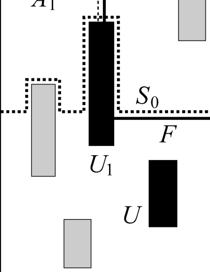
Figure 4.1.

If necessary deforming $\alpha$ by a proper homotopy again, we may assume that that the restriction $\alpha|_{A_{1}\cup\cdots\cup A_{m}}$ is also an embedding. It follows from the fact that any two components of $\overline{\mathbf{T}}\cup\mathbf{T}_{1}^{m}$ are not parallel in $M\!E_{\nu}^{\prime}$ and hence $\alpha|_{A_{i}}$ can not wind around any component of $\overline{\mathbf{T}}\cup\mathbf{T}_{1}^{m}$ homotopically essentially. Thus $F$ is properly isotopic to a surface $F^{\prime}$ in $M\!E_{\nu}^{\prime}\setminus(\overline{U}\cup U_{1}^{m})$ with $F^{\prime}\subset S_{1}\cup A_{1}\cup\cdots\cup A_{m}$ such that $\alpha|_{F^{\prime}}$ is an embedding. This shows that $g|_{F}$ is properly homotopic to an embedding in $N_{\rho}\setminus(\overline{\mathbf{T}}\cup\mathbf{T}_{1}^{m})$. Since $Q_{2},\dots,Q_{2}$ are the components of $N_{\rho}^{\prime}\setminus(g(F)\cup\mathbf{T}_{1}^{m}\cup\overline{\mathbf{T}}$) whose closures in $N_{\rho}^{\prime}\setminus\overline{\mathbf{T}}$ are compact, again by [FHS] $g|_{F}$ is properly homotopic to an embedding in $R\cup(Q_{2}\cup\cdots\cup Q_{m})$. Repeating the same argument repeatedly, one can show that $g|_{F}$ is properly homotopic to an embedding $h$ in $R\cup Q_{u_{1}}\cup\cdots\cup Q_{u_{a}}\subset N_{\rho}[k]$, where $\{Q_{u_{1}},\dots,Q_{u_{a}}\}$ is the subset of $\{Q_{1},\dots,Q_{n}\}$ with $Q_{u_{j}}\cap\mathbb{T}[k]=\emptyset$.

The uniform bi-Lipschitz property for a suitable embedding $h$ is derived easily from geometric limit arguments together with the uniform boundedness of the geometry on $R\cup Q_{u_{1}}\cup\cdots\cup Q_{u_{a}}$. ∎

A horizontal section of $M\!E_{\nu}[k]$ is the union of horizontal surfaces of $M\!E_{\nu}[k]$ in the same level $S\times\{a\}$ for some $a\in\mathbf{R}$. For any horizontal section $\Sigma$ of $M\!E_{\nu}[k]$, let $U_{\Sigma}$ be the union of the components $U$ of $\mathcal{U}[k]\setminus\widehat{\mathcal{U}}$ with $\partial U\cap\Sigma\neq\emptyset$. Then, $\Sigma$ separates $M\!E_{\nu}^{\prime}\setminus U_{\Sigma}$ into the $(+)$ and $(-)$-end components $P_{+},P_{-}$. By Proposition 4.4, $g:M\!E_{\nu}[k]\longrightarrow N_{\rho}[k]$ is properly homotopic to a map $\beta$ such that $\beta|_{\Sigma}$ is an embedding. The map $\beta$ is extended to a proper degree-one map $\widehat{\beta}:M\!E_{\nu}^{\prime}\longrightarrow N_{\rho}^{\prime}$. The embedded surface $\widehat{\beta}(\Sigma)=\beta(\Sigma)$ also separates $N_{\rho}^{\prime}\setminus\mathbf{T}_{\Sigma}$ to the $(+)$ and $(-)$-end components $Q_{+},Q_{-}$, where $\mathbf{T}_{\Sigma}=\widehat{\beta}(U_{\Sigma})=\widehat{g}(U_{\Sigma})$. Since $\widehat{\beta}$ defines a bijection between $\mathcal{U}[k]$ and $\mathbb{T}[k]$, if a component $U$ of $\mathcal{U}[k]$ is in $P_{-}$, then $\widehat{\beta}(P_{+})\cap\mathbf{T}=\emptyset$ for $\mathbf{T}=\widehat{\beta}(U)=\widehat{g}(U)$. Since $\widehat{\beta}(P_{+})\supset Q_{+}$, $\mathbf{T}$ is contained in $Q_{-}$. Similarly, for any component $U$ of $\mathcal{U}[k]\cap P_{+}$, $\widehat{g}(U)$ is contained in $Q_{+}$. This means that the pair $(\Sigma,\beta(\Sigma))$ preserves the orders of $\mathcal{U}[k]$ and $\mathbb{T}[k]$.

Corollary 4.5.

The map $g$ of (4.1) is properly homotopic to a homeomorphism $g_{0}$.

Proof.

Let $\mathcal{H}_{0}$ be a maximal set of horizontal surfaces in $M_{\nu}[k]$ such that any two elements of $\mathcal{H}_{0}$ are not mutually parallel in $M_{\nu}[k]$. From Proposition 4.4 together with the order-preserving property of horizontal surfaces, we know that, for any $F_{1},F_{2}\in\mathcal{H}_{0}$, the restrictions $g|_{F_{1}}$ and $g|_{F_{2}}$ are properly homotopic to mutually disjoint embedded surfaces. By [FHS], $g$ is properly homotopic to a map $g^{\prime}$ such that $g^{\prime}|_{\bigcup_{F\in\mathcal{H}_{0}}F}$ is an embedding, where $g^{\prime}(F)$ has the least area among all surfaces properly homotopic to $g(F)$ on a fixed Riemannian metric on $N_{\rho}[k]$ with respect to which $\partial N_{\rho}[k]$ is locally convex. By using standard arguments in 3-manifold topology (see for example [Wa, He]), one can prove that $g^{\prime}$ is properly homotopic to a homeomorphism $g_{0}$ without moving $g^{\prime}|_{\bigcup_{F\in\mathcal{H}_{0}}F}$. ∎

In [Bow3, Proposition 3.1], this corollary is proved under more general settings. We note that Corollary 4.5 does not necessarily imply that $g_{0}$ is Lipschitz. In fact, since we used the free boundary value problem of the minimal surface theory, we can not control the position of least area surfaces in $N_{\rho}[k]$. For the proof of the bi-Lipschitz model theorem, we need to apply the fixed boundary value problem.

Let $F$ be any horizontal surface in $M_{\nu}[k]$. Since $F\cap\mathcal{U}=F\cap(\mathcal{U}\setminus\mathcal{U}[k])$ and the geometries on all components of $\mathcal{U}\setminus\mathcal{U}[k]$ are uniformly bounded, one can show that any two horizontal surfaces in $M_{\nu}[k]$ with the same topological type are uniformly bi-Lipschitz up to marking.

Remark 4.6 (Technical modifications on $g$).

Since the length of $g(l)$ is at most $K\varepsilon_{1}$ for any boundary component $l$ of a horizontal surface in $M_{\nu}[k]$, we may assume by slightly modifying $g$ that the image $g(\partial F)$ is a disjoint union of closed geodesics in $\partial\mathbb{T}[k]$ for any horizontal surface $F$.

Let $U$ be a component of $\mathcal{U}[k]\setminus\mathcal{U}_{(\widehat{S}\setminus S)}$ and $\mathbf{T}=\widehat{g}(U)$. If $\partial U$ is a torus, then it consists of two horizontal annuli and two vertical annuli. Otherwise, $\partial U$ consists of one horizontal annulus and two vertical half-open annuli. Let $L$ be the set of longitudes $l_{i}$ in $\partial U$ corresponding to the boundary components of these horizontal annuli, $F(l_{i})$ the horizontal surface in $M_{\nu}[k]$ with $\partial F(l_{i})\supset l_{i}$ and $A_{j}$ the horizontal annuli in $\partial U$ with $\partial A_{j}\subset L$. Note that $L$ has either two or four components. We say that $g|_{L}$ is well-ordered if $g|_{\partial U}:\partial U\longrightarrow\partial\mathbf{T}$ is properly homotopic rel. $L$ to a homeomorphism. Since the diameter of any horizontal surface $F$ in $M_{\nu}[k]$ is less than a uniform constant $\delta_{0}$, $\mathrm{diam}_{N_{\rho}[k]}(g(F))<K\delta_{0}$. As in the proof of Proposition 4.4, there exists a proper homotopy for $g$ whose support consists of at most four components of uniformly bounded diameter and which moves $g$ to a map $\gamma$ such that $\gamma|_{\bigcup F(l_{i})\,\cup\,\bigcup A_{j}}$ is an embedding into a small regular neighborhood of $g\bigl{(}\bigcup F(l_{i})\cup\bigcup A_{j}\bigr{)}$ in $N_{\rho}[k]$, see Fig. 4.2.

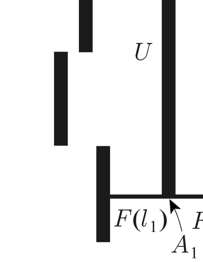
Figure 4.2. The dotted curves in the right side represent $\gamma\bigl{(}\bigcup F(l_{i})\bigr{)}$.

Thus one can modify the Lipschitz map $g$ in a small neighborhood $\mathcal{N}(\partial U)$ of $\partial U$ in $M_{\nu}[k]$ by a uniformly bounded-transferring homotopy so that $g^{\mathrm{new}}|_{\partial U}=\gamma|_{\partial U}$ and hence $g^{\mathrm{new}}|_{L}$ is well-ordered. Here the homotopy being uniformly bounded-transferring means that $\sup_{x\in M_{\nu}[k]}\{\mathrm{dist}_{N_{\rho}[k]}(g(x),\gamma(x))\}$ is less than a uniform constant. The reason why we did not define $g^{\mathrm{new}}=\gamma$ totally in $M_{\nu}[k]$ is to do such a modification of $g$ on each component of $\partial\mathcal{U}[k]$ independently and simultaneously. The Lipschitz constant of $g^{\mathrm{new}}$ may be greater than the original constant, but still denoted by $K$.

Since $N_{\rho}[k]\subset N_{[\varepsilon_{2},\infty)}$ by Theorem 4.1 (i), modifying $g$ again if necessarily, one can suppose that $\mathrm{dist}_{\partial\mathbf{T}}(\partial_{-}A,\partial_{+}A)\geq\varepsilon_{2}/2$ for the closure $A$ of any component of $\partial\mathbf{T}\setminus g(L)$.

4.3. Position of the images of horizontal surfaces

Let $\boldsymbol{\mathcal{Q}}$ be the brick decomposition of $(M_{\nu},\mathcal{U}[k])$. Note that $\boldsymbol{\mathcal{Q}}$ may contain a brick $Q$ the form of which is either $F\times(-\infty,a]$ or $F\times[b,\infty)$ or $S\times\mathbf{R}$. For example, when $Q=F\times[b,\infty)$, $Q$ contains components of $\mathcal{U}\setminus\mathcal{U}[k]$ exiting the end of $Q$. We say that a component of $\partial_{\mathrm{hz}}Q$ contained in $S\times\mathbf{R}$ (resp. in $S\times\{-\infty,\infty\}$) is a real front (resp. an ideal front) of $Q$. Let $\sigma(F)$ be the metric on a horizontal surface $F$ in $Q\in\boldsymbol{\mathcal{Q}}$ induced from that on $M_{\nu}[k]$ and set $\mathrm{dist}(\sigma(F),\sigma(F^{\prime}))=\mathrm{dist}_{\mathrm{Teich}(Q^{S})}(\sigma(F),\sigma(F^{\prime}))$.

Let $F,F^{\prime}$ be horizontal surfaces in $Q\in\boldsymbol{\mathcal{Q}}$. Then $\mathrm{dist}_{M_{\nu}[k]}(F,F^{\prime})$ is the length of a shortest arc $\alpha$ in $M_{\nu}[k]$ connecting $F$ with $F^{\prime}$. However, such an arc $\alpha$ may not be homotopic into $Q$ rel. $\partial\alpha$. So we consider the covering $p:\widetilde{M}_{\nu}[k]\longrightarrow M_{\nu}[k]$ associated to $\pi_{1}(Q)\subset\pi_{1}(M_{\nu}[k])$ and set $\mathrm{dist}_{M_{\nu}[k];Q}(F,F^{\prime})=\mathrm{dist}_{\widetilde{M}_{\nu}[k]}(\widetilde{F},\widetilde{F}^{\prime})$, where $\widetilde{F}$, $\widetilde{F}^{\prime}$ are the lifts of $F$, $F^{\prime}$ to $\widetilde{M}_{\nu}[k]$. One can define $\mathrm{dist}_{N_{\rho}[k];Q}(g(F),g(F^{\prime}))$ and $\mathrm{diam}_{N_{\rho}[k];Q}(g(B))$ for any brick $B$ in $Q$ similarly by using the covering $q:\widetilde{N}_{\rho}[k]\longrightarrow N_{\rho}[k]$ associated to $g_{*}(\pi_{1}(Q))\subset\pi_{1}(N_{\rho}[k])$. Note that, since $B$ is embedded in $Q$, $B$ and its lift to $\widetilde{M}_{\nu}[k]$ have the same diameter.

Lemma 4.7.

For any $d>0$, there exists a uniform constant $\iota(d)$ satisfying the following conditions. Let $F_{j}$ $(j=0,1)$ be horizontal surfaces in $Q\in\boldsymbol{\mathcal{Q}}$ which contains simple non-contractible loops $w_{j}$ of length not greater than $\varepsilon_{1}$. If the geometric intersection number $i(w_{0}^{S},w_{1}^{S})\geq\iota(d)$, then $\mathrm{dist}_{N_{\rho}[k];Q}(g(F_{0}),g(F_{1}))\geq d$.

Proof.

Form the construction of $M_{\nu}[k]$, we know that horizontal surfaces in $Q$ have uniformly bounded geometry up to marking. Since moreover $N_{\rho}[k]\subset N_{\rho[\varepsilon_{2},\infty)}$, a geometric limit argument as in Example 1.3 shows the existence of a uniform constant $\tau(d)>0$ such that, if $d(\sigma(F_{0}),\sigma(F_{1}))\geq\tau(d)$, then $\mathrm{dist}_{N_{\rho}[k];Q}(g(F_{0}),g(F_{1}))\geq d$.

Suppose here that $d(\sigma(F_{0}),\sigma(F_{1}))<\tau(d)$. Then the length of a shortest loop $w_{1}^{\prime}$ in $F_{0}$ freely homotopic to $w_{1}$ in $Q$ is bounded from above by a uniform constant $l(\tau(d))$. Let $\alpha$ be any arc $\alpha$ in $F_{0}$ with $\partial\alpha\subset w_{0}$ such that $\alpha$ is not homotopic in $F$ rel. $\partial\alpha$ to an arc in $w_{0}$. It is not hard to see that the length of $\alpha$ is not less than a uniform constant $\lambda>0$. Since $\lambda i(w_{0}^{S},w_{1}^{S})\leq\mathrm{length}_{F_{0}}(w_{1}^{\prime})<l(\tau(d))$, $\iota(d):=\lambda^{-1}l(\tau(d))$ is our desired uniform constant. ∎

For any brick $Q$ of $\boldsymbol{\mathcal{Q}}$, we will define a new brick decomposition $\boldsymbol{\mathcal{D}}_{Q}$ on $Q$. From the definition of meridian coefficients in Subsection 3.3, we know that, for any component $U$ of $\mathcal{U}\setminus\mathcal{U}[k]$, the diameter of $\partial U$ is less than a uniform constant $\delta_{1}$. We may assume that $\delta_{1}>1$. Let $B$ be any brick of $Q$ such that at least one component $A$ of $\partial_{\mathrm{vt}}B$ is contained in $\partial U$ for some component $U$ of $\mathcal{U}\setminus\mathcal{U}[k]$. Since any point of $B$ is connected with a point of $A$ along a path in a horizontal surface in $B$, the diameter of $B$ is at most $2\delta_{0}+\delta_{1}$. By Lemma 2.3, either the diameter of $Q$ is less than $n_{0}(2\delta_{0}+\delta_{1})$ or there exists a brick $C$ of $\widehat{\mathcal{B}}_{a}$ for some $a$ such that $Q^{S}$ is a compact core of $C^{S}$ and the compliment of $B_{Q}=C\cap Q$ in $Q$ consists of at most two components the closures $B_{\alpha}$ of which are bricks of diameter less than $n_{0}(2\delta_{0}+\delta_{1})$. Hence $\mathrm{diam}_{N_{\rho}[k];Q}(g(B_{\alpha}))$ is less than the uniform constant $Kn_{0}(2\delta_{0}+\delta_{1})=:\gamma_{0}$. These $B_{\alpha}$ are called the complementary brick of $B_{Q}$ in $Q$. Since $\delta_{1}>1$, $\gamma_{0}>K(\delta_{0}+1)$.

According to [Mi1, Lemma 2.1], there exists a uniform constant $d_{0}=d_{0}(2\gamma_{0})$ such that $d_{\mathcal{C}(F)}(u,v)\geq d_{0}$ implies $i(u,v)\geq\iota(2\gamma_{0})$ for any $u,v\in\mathcal{C}_{0}(F)$, where $\iota(\cdot)$ is the uniform constant given in Lemma 4.7. Let $g_{C}$ be the tight geodesic in $C^{S}$ defined in Subsection 2.1. Consider the subsequence $g_{B_{Q}}=\{v_{i}\}_{i\in I}$ of the tight geodesic $g_{C}$ consisting of entries $v_{i}$ with $A(v_{i})\cap\mathrm{Int}B_{Q}\neq\emptyset$, where $I$ is an interval in $\mathbf{Z}$. In the case of $\xi(Q)=1$, one can adjust $B_{Q}$ in $Q$ so that $\mathcal{A}_{g_{B_{Q}}}\cap\partial_{\pm}B_{Q}\neq\emptyset$ if $\partial_{\pm}B_{Q}\neq\emptyset$.

Suppose that the cardinality $|I|$ of $I$ is greater than $2d_{0}$. Then there exists a maximal subsequence $\{i_{j}\}_{j\in J}$ of $I=\{i\}$ with $d_{0}\leq i_{j+1}-j_{j}<2d_{0}$ and containing $\inf I$, $\sup I$ if they are bounded. Consider horizontal surfaces $F_{j}$ $(j\in J)$ in $Q$ such that $F_{j}\subset B_{Q}$ and $F_{j}\cap A(v_{i_{j}})\neq\emptyset$ if $i_{j}\not\in\{\inf I,\sup I\}$ and $F_{j}=\partial_{-}Q$ if $i_{j}=\inf I$, $F_{j}=\partial_{+}Q$ if $i_{j}=\sup I$. Let $\boldsymbol{\mathcal{D}}_{Q}$ be the set of bricks $D_{j}$ in $Q$ with $\partial_{\mathrm{hz}}D_{j}=F_{j}\cup F_{j+1}$. In the case that $|I|\leq 2d_{0}$, we suppose that $\boldsymbol{\mathcal{D}}_{Q}$ is the single point set $\{Q\}$. We denote the union $\bigcup_{Q\in\boldsymbol{\mathcal{Q}}}\boldsymbol{\mathcal{D}}_{Q}$ by $\boldsymbol{\mathcal{D}}$.

For any element of $D$ in $\boldsymbol{\mathcal{D}}_{Q}$ with $\partial_{\mathrm{hz}}D\cap\partial_{\mathrm{hz}}Q=\emptyset$, if $\xi(D)>1$, then $\partial_{-}D$ and $\partial_{+}D$ are connected by the union $R$ of at most $2d_{0}$ bricks in $D$ of diameter not greater than $2\delta_{0}+\delta_{1}$. Since each horizontal surface $F^{\prime}$ of $D$ meets $R$ non-trivially, the diameter of $D$ is less than $2d_{0}(2\delta_{0}+\delta_{1})+2\delta_{0}=:\delta_{2}^{\prime}$. If $\xi(D)=1$, then $D$ contains at most $2d_{0}$ buffer bricks each of which is isometric to either $B_{0,4}$ or $B_{1,1}$. Then one can retake the uniform constant $\delta_{2}^{\prime}$ if necessary so that $\mathrm{diam}(D)<\delta_{2}^{\prime}$ even if $\xi(D)=1$. In the case that $\partial_{\mathrm{hz}}D\cap\partial_{\mathrm{hz}}Q\neq\emptyset$, $D$ contains at most two complementary bricks $B_{\alpha}$. Since $\mathrm{diam}(B_{\alpha})<n_{0}(2\delta_{0}+\delta_{1})$, the diameter of $D$ is less than $\delta_{2}^{\prime}+2n_{0}(2\delta_{0}+\delta_{1})=:\delta_{2}$. It follows that $\delta_{2}$ is a uniform constant with

(4.2) $$\mathrm{diam}(D)<\delta_{2}\quad\mbox{for any $D\in\boldsymbol{\mathcal{D}}$.}$$

Similarly, each component of $\partial_{\mathrm{vt}}D$ is an annulus of diameter less than $\delta_{2}$.

We say that a sequence of horizontal surfaces $\{Y_{l}\}_{l\in L}$ in $Q$ indexed by an interval in $\mathbf{Z}$ ranges in order in $M_{\nu}[k]$ if $\widetilde{Y}_{l-1}$ and $\widetilde{Y}_{l+1}$ are contained in distinct components of $\widetilde{M}_{\nu}[k]\setminus\widetilde{Y}_{l}$ for any $\{l-1,l,l+1\}\subset L$, where $\widetilde{Y}_{u}$ is the lift of $Y_{u}$ to the covering $p:\widetilde{M}_{\nu}[k]\longrightarrow M_{\nu}[k]$ associated to $\pi_{1}(Q)\subset\pi_{1}(M_{\nu}[k])$. The definition of $\{g(Y_{l})\}_{l\in L}$ ranging in order in $N_{\rho}[k]$ is defined similarly when $g(Y_{l})\cap g(Y_{l+1})=\emptyset$ for any $\{l,l+1\}\subset I$.

Lemma 4.8.

Let $Q$ be a element of $\boldsymbol{\mathcal{Q}}$ such that $\boldsymbol{\mathcal{D}}_{Q}$ has at least two elements. Then, for the sequence $\{F_{j}\}_{j\in J}$ of horizontal surfaces in $Q$ as above, $\{g(F_{j})\}$ ranges in order in $N_{\rho}[k]$ and, for any $j\in J$ and $n\in\mathbf{N}$ with $F_{j+n}$ well defined,

(4.3) $$\mathrm{dist}_{N_{\rho}[k];Q}(g(F_{j}),g(F_{j+n}))\geq n\gamma_{0}.$$

Proof.

Set $F_{j}^{\prime}=\partial_{\pm}B_{Q}$ if $F_{j}=\partial_{\pm}Q$ and $F_{j}^{\prime}=F_{j}$ otherwise. Both $F_{j}^{\prime}\cap A(v_{i_{j}})$ and $F_{j+1}^{\prime}\cap A(v_{j_{j+1}})$ contain simple non-contractible loops $w_{1}$, $w_{2}$ of length $\varepsilon_{1}$, respectively. Since $d_{\mathcal{C}(Q^{S})}(w_{1}^{S},w_{2}^{S})=i_{1}\geq d_{0}$, $i(w_{1}^{S},w_{2}^{S})\geq\iota(2\gamma_{0})$. By Lemma 4.7, $\mathrm{dist}_{N_{\rho}[k];Q}(g(F_{j}^{\prime}),g(F_{j+1}^{\prime}))\geq 2\gamma_{0}$. For the proof, we need to consider the case that $F_{u}^{\prime}\neq F_{u}$ or $F_{u+1}^{\prime}\neq F_{u+1}$ for some $u\in J$, say $F_{u}\neq F_{u}^{\prime}$. Then $F_{u+1}^{\prime}=F_{u+1}$ since $\boldsymbol{\mathcal{D}}_{Q}$ has at least two elements. There exists a complementary brick $B_{\alpha}$ with $\partial_{\mathrm{hz}}B_{\alpha}=F_{u}\cup F_{u}^{\prime}$. Since $\mathrm{diam}_{N_{\rho}[k];Q}(g(B_{\alpha}))\leq\gamma_{0}$, $\mathrm{dist}_{N_{\rho}[k];Q}(g(F_{u}),g(F_{u+1}))\geq\gamma_{0}$. It follows that $\mathrm{dist}_{N_{\rho}[k];Q}(g(F_{j}),g(F_{j+1}))\geq\gamma_{0}$ for any $j\in J$.

If $\{g(F_{j}^{\prime}),g(F_{j+1}^{\prime}),g(F_{j+2}^{\prime})\}$ did not range in order in $N_{\rho}[k]$, then for some integer $a$ with $i_{j}\leq a\leq i_{j+2}$, there would exist horizontal surfaces $G_{a}$, $G_{a}^{\prime}$ in $B_{Q}$ with $G_{a}\cap A(v_{a})\neq\emptyset$, $\mathrm{dist}_{M_{\nu}[k];Q}(G_{a},G_{a}^{\prime})\leq 1$ and $g(G_{a}^{\prime})\cap g(F_{j+b}^{\prime})\neq\emptyset$, where $b=2$ if $i_{j}\leq a\leq i_{j+1}$ and $b=0$ if $i_{j+1}\leq a\leq i_{j+2}$. Here $G_{a}^{\prime}$ is taken to be equal to $G_{a}$ unless $\xi(Q)=1$ and $G_{a}^{\prime}$ is in a buffer brick. Since $d_{\mathcal{C}(Q^{S})}(v_{a},v_{i_{j+b}})\geq d_{0}$, Lemma 4.7 would imply $\mathrm{dist}_{N_{\rho}[k];Q}(g(G_{a}),g(F_{j+b}^{\prime}))\geq 2\gamma_{0}$. On the other hand, since $g(G_{a}^{\prime})\cap g(F_{j+b}^{\prime})\neq\emptyset$,

$$\mathrm{dist}_{N_{\rho}[k];Q}(g(F_{j+b}^{\prime}),g(G_{a})) \leq\mathrm{diam}_{N_{\rho}[k];Q}(g(G_{a}^{\prime}))+\mathrm{dist}_{N_{\rho}[k];Q}(g(G_{a}^{\prime}),g(G_{a}))$$

$$\leq K\delta_{0}+K<\gamma_{0}.$$

This contradiction shows that $\{g(F_{j}^{\prime}),g(F_{j+1}^{\prime}),g(F_{j+2}^{\prime})\}$ ranges in order in $N_{\rho}[k]$. Since $\mathrm{dist}_{N_{\rho}[k];Q}(g(F_{v}^{\prime}),g(F_{v+1}^{\prime}))\geq 2\gamma_{0}$ for $v=j,j+1$, $\mathrm{dist}_{N_{\rho}[k];Q}(g(F_{w}),g(F_{w}^{\prime}))\leq\gamma_{0}$ for $w=j,j+2$ and $F_{j+1}^{\prime}=F_{j+1}$, it follows that $\{g(F_{j}),g(F_{j+1}),g(F_{j+2})\}$ also ranges in order and hence $\{g(F_{j})\}$ does. Then the inequality (4.8) is derived immediately from $\mathrm{dist}_{N_{\rho}[k];Q}(g(F_{j}),g(F_{j+1}))\geq\gamma_{0}$ for any $j$. ∎

For any component $U$ of $\mathcal{U}[k]$, $\partial U$ has the foliation $\mathcal{F}_{U}$ consisting of geodesic longitudes of length $\varepsilon_{1}$. By Remark 4.6, the boundary $\partial\mathbf{T}$ of $\mathbf{T}=\widehat{g}(U)$ can have the foliation $\mathcal{G}_{U}$ consisting of geodesic leaves such that $g(l)\in\mathcal{G}_{U}$ for any leaf $l$ of $\mathcal{F}_{U}$. Thus $g|_{\partial U}$ defines a $K$-Lipschitz map $\theta_{U}:\mathcal{F}_{U}\longrightarrow\mathcal{G}_{U}$, where $\mathcal{F}_{U}$ and $\mathcal{G}_{U}$ have the metrics defined by the leaf distance in the Euclidean cylinders $\partial U$ and $\partial\mathbf{T}$ respectively. Any contractible component of $\mathcal{F}_{U}$ or $\mathcal{G}_{U}$ can be identified with an interval in $\mathbf{R}$ as a metric space. For any annulus $A$ in $\partial U$ with geodesic boundary, the subfoliation of $\mathcal{F}_{U}$ with the support $A$ is denoted by $\mathcal{F}_{A}$. When $A$ is vertical, for any $x\in\mathcal{F}_{A}$, the horizontal surface in $M_{\nu}[k]$ which has a boundary component corresponding to $x$ is denoted by $F(x)$. If $F(x)$ is a component of $\partial_{\mathrm{hz}}D$ for some $D\in\boldsymbol{\mathcal{D}}$, then $x$ is called a sectional point.

5. Geometric proof of the bi-Lipschitz model theorem

In this section, we will present a hyperbolic geometric proof of the bi-Lipschitz model theorem given in [BCM].

Theorem 5.1 (Bi-Lipschitz Model Theorem).

There exist uniform constants $K^{\prime}\geq 1,k>0$ such that there is a marking-preserving $K^{\prime}$-bi-Lipschitz homeomorphism $\varphi:M\!E_{\nu}[k]\longrightarrow N_{\rho}[k]$ which can be extended to a conformal homeomorphism from $\partial_{\infty}M\!E_{\nu}$ to $\partial_{\infty}N$.

For the proof, we need the following two lemmas.

Lemma 5.2.

For any component $U$ of $\mathcal{U}[k]$, let $A$ be a vertical component of $\partial U$. Then there exists a uniform constant $a_{0}$ such that, for any $x_{0},x_{1}\in\mathcal{F}_{A}$ with $\mathrm{dist}_{\mathcal{F}_{U}}(x_{0},x_{1})\geq a_{0}$, $\mathrm{dist}_{\mathcal{G}_{U}}(\theta_{U}(x_{0}),\theta_{U}(x_{1}))\geq K$.

Proof.

Since each component of $\partial_{\mathrm{vt}}D$ $(D\in\boldsymbol{\mathcal{D}})$ has diameter less than $\delta_{2}$, for any $x_{i}\in\mathcal{F}_{A}$, there exists a sectional point $y_{i}\in\mathcal{F}_{A}$ with $|x_{i}-y_{i}|\leq\delta_{2}/2$. Since $\theta_{U}$ is $K$-Lipschitz, it suffices to show that there exists a uniform constant $a_{0}$ with $|y_{0}-y_{1}|<a_{0}-\delta_{2}$ for any sectional points $y_{0},y_{1}$ in $\mathcal{F}_{A}$ with $|\theta_{U}(y_{0})-\theta_{U}(y_{1})|<K(\delta_{2}+1)$. We may assume that $y_{0}<y_{1}$ and $\theta_{U}(y_{0})\leq\theta_{U}(y_{1})$. Consider the annulus $A^{\prime}$ in $\partial\mathbf{T}$ with $\mathcal{G}_{A^{\prime}}=[\theta_{U}(y_{0}),\theta_{U}(y_{1})]$, where $\mathbf{T}=\widehat{g}(U)$. Set $X=g(F(y_{0}))\cup A^{\prime}\cup g(F(y_{1}))$. Since $\mathrm{diam}_{N_{\rho}[k];Q}(g(F(y_{i})))\leq K\delta_{0}$ for $i=0,1$, $\mathrm{diam}(X)<K(2\delta_{0}+\delta_{2}+1)$.

Suppose that $g(F(y))\cap X$ is empty for some sectional point $y\in(y_{0},y_{1})$. We may assume that $\theta_{U}(y)<\theta_{U}(y_{0})$. Since $g$ is properly homotopic to a homeomorphism $g_{0}$ by Corollary 4.5, one can exchange the positions of $g(F(y))$ and $g(F(y_{0}))$ by a proper homotopy in $N_{\rho}[k]$. If necessary modifying $g_{0}$ near $A$, we may assume that $g_{0}(\partial_{A}F(y_{0}))=g(\partial_{A}F(y_{0}))$, where $\partial_{A}F(y_{0})=F(y_{0})\cap A$. Since $g(F(y))\cap g(F(y_{0}))=\emptyset$ and $g_{0}(F(y_{0}))\cap g_{0}(F(y))=\emptyset$, by [FHS] there exist properly embedded mutually disjoint surfaces $H_{y}$, $H_{y_{0}}$, $H_{y}^{\prime}$ in $N_{\rho}[k]$ such that $g(F(y))$ is properly homotopic to $H_{y}$ rel. $g(\partial_{A}F(y))$, both $g(F(y_{0}))$ and $g_{0}(F(y_{0}))$ to $H_{y_{0}}$ rel. $g(\partial_{A}F(y_{0}))$, and $g_{0}(F(y))$ to $H_{y}^{\prime}$ rel. $g_{0}(\partial_{A}F(y))$. Since $H_{y}\cup H_{y}^{\prime}$ excises from $N_{\rho}[k]$ a topological brick $B$ containing $H_{y_{0}}$ as a proper subsurface, $H_{y}$ is properly homotopic to $H_{y_{0}}$ in $N_{\rho}[k]$. This implies that $F(y)$ and $F(y_{0})$ are properly homotopic to each other in $M_{\nu}[k]$ and hence contained in the same brick $Q\in\boldsymbol{\mathcal{Q}}$.

Let $Z$ be the set of sectional points $z$ of $\mathcal{F}_{A\cap Q}$ with $z>y_{0}$. By Lemma 4.8, $\theta_{U}(z_{+})<\theta_{U}(y_{0})$ and $\theta_{U}(Z)$ is contained in the interval $[\theta_{U}(z_{+}),\theta_{U}(y_{0}))$, where $F(z_{+})\subset\partial_{+}Q$. Since $\theta_{U}(z)<\theta_{U}(y_{1})$ for any $z\in Z$, $y_{1}$ is not in $Z$. If $y^{\prime}$ is the smallest sectional point in $(z_{+},y_{1}]$, then $g(F(y^{\prime}))$ meets $X$ non-trivially. Let $A^{\prime\prime}$ be the annulus in $\partial\mathbf{T}$ with $\mathcal{G}_{A^{\prime\prime}}=[\theta_{U}(z_{+}),\theta_{U}(y^{\prime})]$ (or $[\theta_{U}(y^{\prime}),\theta_{U}(z_{+})]$) and $Y=A^{\prime\prime}\cup g(F(y^{\prime}))$. Since $\mathrm{diam}(A^{\prime\prime})\leq K\delta_{2}$, $\mathrm{diam}(Y)\leq K(\delta_{0}+\delta_{2})$. If $g(F(z))\cap Y=\emptyset$ for $z\in Z$, then the positions of $g(F(y^{\prime}))$ and $g(F(z))$ would be exchanged by proper homotopy in $N_{\rho}[k]$. This contradicts that $y^{\prime}\not\in Z$. Hence $g(F(z))$ intersects $X^{\prime}=\mathcal{N}_{K(\delta_{0}+\delta_{2})}(X,N_{\rho}[k])$. It follows that $g(F(y))\cap X^{\prime}\neq\emptyset$ for any sectional point $y$ in $[y_{0},y_{1}]$.

The interval $[y_{0},y_{1}]$ has at least $(y_{1}-y_{0}-\delta_{2})/\delta_{2}$ sectional points $y_{\alpha}$. Since the surfaces $F(y_{\alpha})$ have mutually non-parallel simple non-contractible loops $l_{\alpha}$ with $\mathrm{length}_{N_{\rho}[k]}(g(l_{\alpha}))\leq K\varepsilon_{1}$ and $\mathrm{diam}(X^{\prime})$ is uniformly bounded, by a geometric limit argument as in Example 1.3, one can prove that $(y_{1}-y_{0}-\delta_{2})/\delta_{2}$ is less than a uniform constant $m_{0}$. Thus we have $|y_{0}-y_{1}|<a_{0}-\delta_{2}$ for $a_{0}:=(m_{0}+2)\delta_{2}$. ∎

For an interval $J$ in $\mathcal{F}_{U}$, an interval $I$ in $\mathcal{G}_{U}$ with $\partial I=\theta_{U}(\partial J)$ is the reduced image of $J$ if $\theta_{U}|_{J}$ is homotopic rel. $\partial J$ to a homeomorphism to $I$.

Lemma 5.3.

There exist uniform constants $K_{0},d_{3}$ such that $\theta_{U}$ is homotopic to a $K_{0}$-bi-Lipschitz map $\zeta_{U}:\mathcal{F}_{U}\longrightarrow\mathcal{G}_{U}$ such that $\mathrm{dist}_{\mathcal{G}_{U}}(\theta_{U}(x),\zeta_{U}(x))<d_{3}$ for any $x\in\mathcal{F}_{U}$.

Proof.

Consider any component $U\in\mathcal{U}[k]$ such that $\partial U$ contains a vertical annulus component $A$ with $\mathrm{diam}_{\mathcal{F}_{U}}(\mathcal{F}_{A})\geq a_{0}$. Let $\{x_{i}\}$ be a sequence in $\mathcal{F}_{A}$ with $a_{0}\leq x_{i+1}-x_{i}\leq 2a_{0}$ and $\mathcal{F}_{A}=\bigcup_{i}J_{i}$, where $J_{i}=[x_{i},x_{i+1}]$. By Lemma 5.2, the reduced image $I_{i}$ of $J_{i}$ satisfies

(5.1) $$K\leq\mathrm{diam}_{\mathcal{G}_{U}}(I_{i})\leq\mathrm{diam}_{\mathcal{G}_{U}}(\theta_{U}(J_{i}))\leq 2Ka_{0}.$$

Thus $\theta_{U}|_{\mathcal{F}_{A}}:\mathcal{F}_{A}\longrightarrow\mathcal{G}_{U}$ is homotopic to the map $\zeta_{A}:\mathcal{F}_{A}\longrightarrow\mathcal{G}_{U}$ rel. $\{x_{i}\}$ such that, for any $J_{i}$, the restriction $\zeta_{A}|_{J_{i}}$ is an affine map onto $I_{i}$. Then, by (5.1), $\mathrm{dist}_{\mathcal{G}_{U}}(\theta_{U}(x),\zeta_{A}(x))<2Ka_{0}$ for any $x\in\mathcal{F}_{A}$. If $I_{i}\cap I_{i+1}\setminus\{x_{i+1}\}$ were not empty, then there would exist $z_{i}\in J_{i}$ and $z_{i+1}\in J_{i+1}$ with $\max\{x_{i+1}-z_{i},z_{i+1}-x_{i+1}\}=a_{0}$ and $\theta_{U}(z_{i})=\theta_{U}(z_{i+1})$. Since $z_{i+1}-z_{i}\geq a_{0}$, this contradicts Lemma 5.2. Thus, by (5.1), $\zeta_{A}$ is a uniformly bi-Lipschitz map onto an interval in $\mathcal{G}_{U}$.

Let $A^{\prime}$ be a horizontal component of $\partial U$. If $A^{\prime}$ is not contained in a boundary brick in $\boldsymbol{\mathcal{B}}_{\partial}$, then $A^{\prime}$ is isometric to $S^{1}(\varepsilon_{1})\times[0,1]$ as defined in Subsection 3.1 and hence $\mathrm{diam}_{\mathcal{F}_{U}}(\mathcal{F}_{A^{\prime}})=1$. By Remark 4.6, the reduced image $I$ of $\mathcal{F}_{A^{\prime}}$ satisfies

$$\frac{\varepsilon_{2}}{2}\leq\mathrm{diam}_{\mathcal{G}_{U}}(I)\leq\mathrm{diam}_{\mathcal{G}_{U}}(\theta_{U}(\mathcal{F}_{A^{\prime}}))\leq K.$$

Thus $\theta_{U}|_{\mathcal{F}_{A^{\prime}}}:\mathcal{F}_{A^{\prime}}\longrightarrow\mathcal{G}_{U}$ is homotopic to a uniformly bi-Lipschitz map $\zeta_{A^{\prime}}:\mathcal{F}_{A^{\prime}}\longrightarrow I^{\prime}\subset\mathcal{G}_{U}$ rel. $\partial\mathcal{F}_{A^{\prime}}$ by a uniformly bounded-transferring homotopy. If $A^{\prime}$ is contained in a boundary brick, then $\zeta_{A^{\prime}}=\theta_{U}|_{A^{\prime}}:A^{\prime}\longrightarrow\mathcal{G}_{U}$ is already uniformly bi-Lipschitz onto the image by Theorem 4.1 (iii). The union $\zeta_{U}$ of these bi-Lipschitz maps is our desired map. ∎

Proof of Theorem 5.1.

By Lemma 5.3, there exists a uniform constant $K_{1}$ such that $g:M\!E_{\nu}[k]\longrightarrow N_{\rho}[k]$ is properly homotopic to a $K_{1}$-Lipschitz map $g_{1}$ with $\mathrm{dist}_{N_{\rho}[k]}(g(x),g_{1}(x))\leq d_{3}+1$ for any $x\in M\!E_{\nu}[k]$ and such that the restriction $g_{1}|_{\partial U}$ induces the $K_{1}$-bi-Lipschitz map $\zeta_{U}:\mathcal{F}_{U}\longrightarrow\mathcal{G}_{U}$ for any component $U$ of $\mathcal{U}[k]$, where the support of the homotopy is contained in a small collar neighborhood of $\partial\mathcal{U}[k]$ in $M\!E_{\nu}[k]$. Here ‘$+1$’ just means that $d_{3}+1$ is a constant strictly greater than $d_{3}$. Since the original $g|_{E_{\nu}}:E_{\nu}\longrightarrow E_{N}$ is uniformly bi-Lipschitz by Theorem 4.1 (iii), we may suppose that $g_{1}|_{E_{\nu}}$ is also a uniformly bi-Lipschitz map onto $E_{N}$.

Deform the metric on $N_{\rho}[k]$ in a small collar neighborhood of $\partial N_{\rho}[k]$ so that $\partial N_{\rho}[k]$ is locally convex but the sectional curvature of $N_{\rho}[k]$ is still pinched by $-1$ and some uniform constant $\kappa_{0}>0$. For any critical horizontal surface $G_{\alpha}$ of $M\!E_{\nu}[k]$, let $H_{\alpha}$ be a surface in $N_{\rho}[k]$ which has the least area with respect to the modified metric on $N_{\rho}[k]$ among all surfaces properly homotopic to $g_{1}(G_{\alpha})$ without moving their boundaries. By Proposition 4.4, $g_{1}(G_{\alpha})$ is properly homotopic to an embedding without moving the boundary. By [FHS], $H_{\alpha}$ is also an embedded surface and $H_{\alpha}\cap H_{\beta}=\emptyset$ whenever $H_{\alpha}\neq H_{\beta}$. Since the area of $G_{\alpha}$ is less than some uniform constant $A_{0}$, $\mathrm{Area}(H_{\alpha})\leq\mathrm{Area}(g_{1}(G_{\alpha}))\leq K_{1}^{2}A_{0}$. Since $N_{\rho}[k]\subset N_{\rho[\varepsilon_{2},\infty)}$ by Theorem 4.1 (i), the injectivity radius of $H_{\alpha}$ is not less than $\varepsilon_{2}$. Since moreover the intrinsic curvature of $H_{\alpha}$ at any point is at most $\kappa_{0}$, the diameter of $H_{\alpha}$ is less than a uniform constant. As was seen in Example 1.4 and Remark 1.5, there exists a uniform constant $K_{2}>1$ such that $g_{1}$ is homotopic without moving $g_{1}|_{\partial M\!E_{\nu}[k]}$ to a $K_{2}$-Lipschitz map $g_{2}$ the restriction $g_{2}|_{G_{\alpha}}$ of which is a $K_{2}$-bi-Lipschitz map onto $H_{\alpha}$ for any $G_{\alpha}$.

Let $\{F_{j}\}$ be the sequence of horizontal surfaces in $Q\in\boldsymbol{\mathcal{Q}}$ given in Lemma 4.8. Since $g_{2}$ is obtained from $g$ by a uniformly bounded-transferring homotopy, there exists a uniform constant $a_{1}\in\mathbf{N}$ and a subsequence $\mathcal{Y}_{Q}=\{Y_{l}\}_{l\in L}$ of $\{F_{j}\}$ with $Y_{l}=F_{j_{l}}$ indexed by an interval $L$ in $\mathbf{Z}$ which satisfies the following conditions if $\boldsymbol{\mathcal{D}}_{Q}$ contains at least $(a_{1}-1)$ bricks.

1. $Y_{\inf L}=\partial_{-}Q$ and $Y_{\sup L}=\partial_{+}Q$ if any.

2. $j_{l+1}-j_{l}\leq a_{1}$ and $\mathrm{dist}_{N_{\rho}[k];Q}(g_{2}(Y_{l}),g_{2}(Y_{l+1}))\geq 3\gamma_{0}$ for any $\{l,l+1\}\subset L$.

3. The sequence $\{g_{2}(Y_{l})\}$ ranges in order from $g_{2}(\partial_{-}Q)$ to $g_{2}(\partial_{+}Q)$ in $N_{\rho}[k]$.

By (4.2) and (ii), $\mathrm{dist}_{N_{\rho}[k];Q}(g_{2}(Y_{l}),g_{2}(Y_{l+1}))\leq K_{2}\delta_{2}a_{1}$. Set $\mathcal{Y}=\bigcup_{Q\in\boldsymbol{\mathcal{Q}}}\mathcal{Y}_{Q}$. Note that the $\gamma_{0}$-neighborhoods $\mathcal{N}_{\gamma_{0}}(g_{2}(Y_{u}))$ of $g_{2}(Y_{u})$ in $N_{\rho}[k]$ for $Y_{u}\in\mathcal{Y}_{Q}$ not in $\partial_{\mathrm{hz}}Q$ are mutually disjoint and disjoint from the $\gamma_{0}$-neighborhood of $g_{2}(\partial_{\mathrm{hz}}Q)$. By Proposition 4.4, for any $Y_{u}\in\mathcal{Y}\setminus\bigcup_{\alpha}\{G_{\alpha}\}$, the restriction $g_{2}|Y_{u}:Y_{u}\longrightarrow N_{\rho}[k]$ is properly homotopic to an embedding $h_{u}$ which is a $K_{3}$-bi-Lipschitz map onto a surface contained in $\mathcal{N}_{\gamma_{0}}(g_{2}(Y_{u}))$ for some uniform constant $K_{3}\geq 1$. Since the geometries on these embedded surfaces are uniformly bounded, there exists a uniform constant $K^{\prime}\geq\max\{K_{2},K_{3}\}$ as in Example 1.4 such that $g_{2}$ is properly homotopic to a $K^{\prime}$-bi-Lipschitz map $\varphi$ with $\varphi|_{\bigcup_{\alpha}G_{\alpha}}=g_{2}|_{\bigcup_{\alpha}G_{\alpha}}$ and $\varphi|_{Y_{u}}=h_{u}$ for any $Y_{u}\in\mathcal{Y}\setminus\{G_{\alpha}\}$. This completes the proof. ∎

It is well known that the bi-Lipschitz model theorem together with standard hyperbolic geometric arguments implies the Ending Lamination Conjecture.

Theorem 5.4 (Ending Lamination Conjecture).

Let $N_{\rho},N_{\rho^{\prime}}$ be hyperbolic $3$-manifolds as in Subsection 1.2 which have the same end invariant set $\nu$. Then, any marking-preserving homeomorphism $f:N_{\rho}\longrightarrow N_{\rho^{\prime}}$ is properly homotopic to an isometry.

Proof.

By Theorem 5.1, there exist marking-preserving uniformly bi-Lipschitz maps $\varphi:M\!E_{\nu}[k]\longrightarrow N_{\rho}[k]$ and $\varphi^{\prime}:M\!E_{\nu}[k]\longrightarrow N_{\rho^{\prime}}[k]$ which are extended to conformal homeomorphisms from $\partial_{\infty}M\!E_{\nu}[k]$ to $\partial_{\infty}N_{\rho}$ and $\partial_{\infty}N_{\rho^{\prime}}$ respectively. One can furthermore extend $\varphi,\varphi^{\prime}$ to uniformly bi-Lipschitz maps $\widehat{\varphi}:M\!E_{\nu}\longrightarrow N_{\rho}$ and $\widehat{\varphi}^{\prime}:M\!E_{\nu}\longrightarrow N_{\rho^{\prime}}$ by using standard arguments of hyperbolic geometry, for example see [BCM, Lemma 8.5] or [Bow3, Lemma 5.8]. Then $\Phi=\widehat{\varphi}^{\prime}\circ\widehat{\varphi}^{-1}:N_{\rho}\longrightarrow N_{\rho^{\prime}}$ is a marking-preserving bi-Lipschitz map. The $\Phi$ is lifted to a bi-Lipschitz map $\widetilde{\Phi}:\mathbf{H}^{3}\longrightarrow\mathbf{H}^{3}$ between the universal coverings, which is equivariant with respect to the covering transformations. The map $\widetilde{\Phi}$ is extended to a quasi-conformal homeomorphism $\widetilde{\Phi}_{\partial}$ on the Riemann sphere $\widehat{\mathbf{C}}$ such that $\widetilde{\Phi}_{\partial}|_{\Omega_{\rho}}$ is a conformal homeomorphism from $\Omega_{\rho}$ to $\Omega_{\rho^{\prime}}$, where $\Omega_{\rho}$ is the domain of discontinuity of the Kleinian group $\rho(\pi_{1}(S))$. By Sullivan’s Rigidity Theorem [Su], $\widetilde{\Phi}_{\partial}$ is an equivariant conformal map on $\widehat{\mathbf{C}}$ and hence extended to an equivariant isometry $\widetilde{\Psi}:\mathbf{H}^{3}\longrightarrow\mathbf{H}^{3}$, which covers an isometry $\psi:N_{\rho}\longrightarrow N_{\rho^{\prime}}$ properly homotopic to $f$. ∎

References

- [BP] R. Benedetti and C. Petronio, Lectures on hyperbolic geometry, Universitext, Springer-Verlag, Berlin, 1992.
- [Bo] F. Bonahon, Bouts des variétés hyperboliques de dimension , Ann. of Math. 124 (1986) 71-158.
- [Bow1] B. Bowditch, Intersection numbers and the hyperbolicity of the curve complex, J. Reine Angew. Math. 598 (2006) 105-129.
- [Bow2] B. Bowditch, Length bounds on curves arising from tight geodesics, Geom. Funct. Anal. 17 (2007) 1001-1042.
- [Bow3] B. Bowditch, Geometric models for hyperbolic 3-manifolds, preprint (2006).
- [BBES] J. Brock, K. Bromberg, R. Evans and J. Souto, in preparation.
- [BCM] J. Brock, R. Canary and Y. Minsky, The classification of Kleinian surface groups, II: The Ending Lamination Conjecture, E-print math.GT/0412006.
- [FHS] M. Freedman, J. Hass and P. Scott, Least area incompressible surfaces in -manifolds, Invent. Math. 71 (1983) 609-642.
- [Ham] U. Hamenstädt, Train tracks and the Gromov boundary of the complex of curves, Spaces of Kleinian groups, pp. 187-207, London Math. Soc. Lecture Note Ser., 329, Cambridge Univ. Press, Cambridge, 2006.
- [Har] W. Harvey, Boundary structure of the modular group, Riemann surfaces and related topics: Proceedings of the 1978 Stony Brook Conference (State Univ. New York, Stony Brook, N.Y., 1978), pp. 245-251, Ann. of Math. Studies No. 97, Princeton Univ. Press, Princeton, N.J. 1981.
- [HS] J. Hass and P. Scott, The existence of least area surfaces in -manifolds, Trans. Amer. Math. Soc. 310 (1988) 87-114.
- [He] J. Hempel, -Manifolds, Ann. of Math. Studies, No. 86, Princeton Univ. Press, Princeton, N.J. 1976.
- [JM] T. Jørgensen and A. Marden, Geometric and algebraic convergence of Kleinian groups, Math. Scand. 66 (1990) 47-72.
- [Kla] E. Klarreich, The boundary at infinity of the curve complex and the relative Teichmüller space, preprint (1999).
- [Ma] A. Marden, Outer Circles: An introduction to hyperbolic -manifolds, Cambridge Univ. Press, 2007.
- [MM1] H. Masur and Y. Minsky, Geometry of the complex of curves, I: Hyperbolicity, Invent. Math. 138 (1999) 103-149.
- [MM2] H. Masur and Y. Minsky, Geometry of the complex of curves, II: Hierarchical structure., Geom. Funct. Anal. 10 (2000) 902-974.
- [MT] K. Matsuzaki and M. Taniguchi, Hyperbolic manifolds and Kleinian groups, Oxford Univ. Press (1998).
- [Mi1] Y. Minsky, Bounded geometry for Kleinian groups, Invent. Math. 146 (2001) 143-192.
- [Mi2] Y. Minsky, The classification of Kleinian surface groups I: models and bounds, Ann. of Math. (to appear).
- [OS] K. Ohshika and T. Soma, Geometry and topology of geometric limits I, in preparation.
- [Ot] J.-P. Otal, Sur le nouage des géodésiques dans les variétés hyperboliques, C. R. Acad. Sci. Paris Ser. I Math. 320 (1995) 847-852.
- [Re] M. Rees, The ending laminations theorem direct from Teichmüller geodesics, E-print math/0404007 v5.
- [So] T. Soma, Geometric limits and length bounds on curves, preprint.
- [Su] D. Sullivan, On the ergodic theory at infinity of an arbitrary discrete group of hyperbolic motions, Riemann surfaces and related topics, Proceedings of the 1978 Stony Brook Conference (State Univ. New York, Stony Brook, N.Y., 1978) pp. 465-496, Ann. of Math. Stud., 97, Princeton Univ. Press, Princeton, N.J., 1981.
- [Th1] W. Thurston, The geometry and topology of -manifolds, Lecture Notes, Princeton Univ., Princeton (1978), on line at http://www.msri.org/publications/books/gt3m/.
- [Th2] W. Thurston, Three dimensional manifolds, Kleinian groups and hyperbolic geometry, Bull. Amer. Math. Soc. 6 (1982) 357-381.
- [Wa] F. Waldhausen, On irreducible -manifolds which are sufficiently large, Ann. of Math. 87 (1968) 56-88.