Algorithms for Temperature-Aware Task
Scheduling in Microprocessor Systems

Abstract

We study scheduling problems motivated by recently developed techniques for microprocessor thermal management at the operating systems level. The general scenario can be described as follows. The microprocessor’s temperature is controlled by the hardware thermal management system that continuously monitors the chip temperature and automatically reduces the processor’s speed as soon as the thermal threshold is exceeded. Some tasks are more CPU-intensive than other and thus generate more heat during execution. The cooling system operates non-stop, reducing (at an exponential rate) the deviation of the processor’s temperature from the ambient temperature. As a result, the processor’s temperature, and thus the performance as well, depends on the order of the task execution. Given a variety of possible underlying architectures, models for cooling and for hardware thermal management, as well as types of tasks, this scenario gives rise to a plethora of interesting and never studied scheduling problems.

We focus on scheduling real-time jobs in a simplified model for cooling and thermal management. A collection of unit-length jobs is given, each job specified by its release time, deadline and heat contribution. If, at some time step, the temperature of the system is $\tau$ and the processor executes a job with heat contribution $h$, then the temperature at the next step is $(\tau+h)/2$. The temperature cannot exceed the given thermal threshold $T$. The objective is to maximize the throughput, that is, the number of tasks that meet their deadlines. We prove that, in the offline case, computing the optimum schedule is NP-hard, even if all jobs are released at the same time. In the online case, we show a $2$-competitive deterministic algorithm and a matching lower bound.

1 Introduction

Background.

The problem of managing the temperature of processor systems is not new; in fact, the system builders had to deal with this challenge since the inception of computers. Since early 1990s, the introduction of battery-operated laptop computers and sensor systems highlighted the related issue of controlling the energy consumption.

Most of the initial work on these problems was hardware and systems oriented, and only during the last decade substantial progress has been achieved on developing models and algorithmic techniques for microprocessor temperature and energy management. This work proceeded in several directions. One direction is based on the fact that the energy consumption is a fast growing function of the processor speed (or frequency). Thus we can save energy by simply slowing down the processor. Here, algorithmic research focussed on speed scaling – namely dynamically adjusting the processor speed over time to optimize the energy consumption while ensuring that the system meets the desired performance requirements. Another technique (applicable to the whole system, not just the microprocessor) involves power-down strategies, where the system is powered-down or even completely turned off when some of its components are idle. Since changing the power level of a system introduces some overhead, scheduling the work to minimize the overall energy usage in this model becomes a challenging optimization problem.

Models have also been developed for the processor’s thermal behavior. Here, the main objective is to ensure that the system’s temperature does not exceed the so-called thermal threshold, above which the processor cannot operate correctly, or may even be damaged. In this direction, techniques and algorithms have been proposed for using speed-scaling to optimize the system’s performance while maintaining the temperature below the threshold.

We refer the reader to the survey by Irani and Pruhs [5], and references therein, for more in-depth information on the models and algorithms for thermal and energy management.

Temperature-aware scheduling.

The above models address energy and thermal management at the micro-architecture level. In contrast, the problem we study in this paper addresses the issue of thermal management at the operating systems level. Most of the previous work in this direction focussed on multi-core systems, where one can move tasks between the processors to minimize the maximum temperature [9, 1, 2, 6, 7, 8, 4, 10]. However, as it has been recently discovered, even in single-core systems one can exploit variations in heat contributions among different tasks to reduce the processor’s temperature through appropriate task scheduling [1, 4, 6, 7, 11]. In this scenario, the microprocessor’s temperature is controlled by the hardware dynamic thermal management (DTM) system that continuously monitors the chip temperature and automatically reduces the processor’s speed as soon as the thermal threshold (maximum safe operating temperature) is exceeded. Typically, the frequency is reduced by half, although it can be further reduced to one fourth or even one eighth, if needed. Running at a lower frequency, the CPU generates less heat. The cooling system operates non-stop, reducing (at an exponential rate) the deviation of the processor’s temperature from the ambient temperature. Once the chip cools down to below the threshold, the frequency is increased again.

Different tasks use different microprocessor units in different ways; in particular, some tasks are more CPU-intensive than other. As a result, the processor’s thermal behavior – and thus the performance as well – depends on the order of the task execution. In particular, Yang et al.  [11] point out that, based on the standard model for the microprocessor thermal behavior, for any given two tasks, scheduling the “hotter” job before the “cooler” one, results in a lower final temperature than after the reverse order. They take advantage of this phenomenon to reduce the number of DTM invocations, thus improving the performance of the OS scheduler.

With multitudes of possible underlying architectures (for example, single- vs. multi-core systems), models for cooling and hardware thermal management, as well as types of jobs (real-time, batch, etc.), the scenario outlined above gives rise to a plethora of interesting and never yet studied scheduling problems.

Our model.

We focus on scheduling real-time jobs in a somewhat simplified model for cooling and thermal management. The time is divided into unit time slots and each job has unit length. (These jobs represent unit slices of the processes present in the OS scheduler’s queue.) We assume that the heat contributions of these jobs are known. This is counterintuitive, but reasonably realistic, for, as discussed in [11], these values can be well approximated using appropriate prediction methods.

In our thermal model we assume, without loss of generality, that the ambient temperature is $0$ and that the heat contributions are expressed in the units of temperature (that is, by how much they would increase the chip temperature in the absence of cooling). In reality [11], during the execution of a job, its heat contribution is spread over the whole time slot and so is the effect of cooling; thus, the final temperature can be expressed using an integral function. In this paper, we use a simplified model where we first take into account the job’s heat contribution, and then apply the cooling, where the cooling simply reduces the temperature by half.

Finally, we assume that only one processor frequency is available. Consequently, if there is no job whose execution does not cause a thermal violation, the processor must stay idle through the next time slot.

Our results.

Summarizing, our scheduling problem can be now formalized as follows. A collection of unit-length jobs is given, each job $j$ with a release time $r_{j}$, deadline $d_{j}$ and heat contribution $h_{j}$. If, at some time step, the temperature of the system is $\tau$ and the processor executes a job $j$, then the temperature at the next step is $(\tau+h_{j})/2$. The temperature cannot exceed the given thermal threshold $T$. The objective is to compute a schedule which maximizes the number of tasks that meet their deadlines.

We prove that in the offline case computing the optimum schedule is NP-hard, even if all jobs are released at the same time and have equal deadlines. In the online case, we show a $2$-competitive deterministic algorithm and a matching lower bound.

2 Terminology and Notation

The input consists of $n$ unit-length jobs that we number $1,2,\ldots,n$. Each job $j$ is specified by a triple $(r_{j},d_{j},h_{j})\in\mathbb{N}\times\mathbb{N}\times\mathbb{Q}$, where $r_{j}$ is its release time, $d_{j}$ is the deadline and $h_{j}$ is its heat contribution. The time is divided into unit-length slots and each job can be executed in any time slot in the interval $[r_{j},d_{j}]$. By $\tau_{u}$ we denote the processor temperature at time $u$. The initial temperature is $\tau_{0}=0$, and it changes according to the following rules: if the temperature of the system at a time $u$ is $\tau_{u}$ and the processor executes a job $j$ then the temperature at time $u+1$ is $\tau_{u+1}=(\tau_{u}+h_{j})/2$. The temperature cannot exceed the given thermal threshold $T$. Without loss of generality, we assume that $T=1$. Thus if $(\tau_{u}+h_{j})/2>1$ then $j$ cannot be executed at time $u$. Idle slots are treated as executing a job with heat contribution $0$, that is, after an idle slot the temperature decreases by half.

Given an instance, as above, the objective is to compute a schedule with maximum throughput, where throughput is defined as the number of completed jobs. Extending the standard notation for scheduling problems, we denote the offline version of this problem by $1|r_{i},h_{i},p_{i}=1|\sum U_{i}$.

In the online version, denoted $1|\textrm{online-}r_{i},h_{i},p_{i}=1|\sum U_{i}$, jobs are available to the algorithm at their release time. Scheduling decisions of the algorithm cannot depend on the jobs that have not yet been released.

Example.

Suppose we have four jobs, specified in notation $j\to(r_{j},d_{j},h_{j})$: $1\to(0,2,0.4)$, $2\to(0,4,0.6)$, $3\to(2,3,1.9)$, $4\to(4,6,0.8)$.

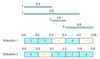
Figure 1: Example of two schedules.

Figure 1 shows these jobs and two schedules. Numbers above the schedules denote temperatures. In the first schedule, when we schedule job $2$ at time $1$, the processor is too hot to execute job $3$, so it will not complete job $3$ at all. In the second schedule, we stay idle in step 2, allowing us to complete all jobs.

3 The NP-Completeness Proofs

In this section we prove that the scheduling problem $1|r_{i},h_{i},p_{i}=1|\sum U_{i}$ is NP-hard. For the sake of exposition, we start with a proof for the general case, and later we give a proof for the special case when all release times and deadlines are equal.

Theorem 1

The offline problem $1|r_{i},h_{i},p_{i}=1|\sum U_{i}$ is NP-hard.

Proof: We use a reduction from the 3-Partition problem, defined as follows: we are given a set $S$ of $3n$ positive integers $a_{1},\ldots,a_{3n}$ such that $\beta/4<a_{i}<\beta/2$ for all $i$, where $\beta=\frac{1}{n}\sum a_{i}$. The goal is to partition $S$ into $n$ subsets, each subset with the total sum equal exactly $\beta$. (By the assumption on the $a_{i}$, each subset will have to have exactly $3$ elements.) This partition of $S$ will be called a $3$-partition. 3-Partition is well-known to be NP-hard [3] in the strong sense, that is, even if $\max_{i}a_{i}\leq p(n)$, for some polynomial $p(n)$.

We now describe the reduction. For the given instance of 3-Partition we construct an instance of $1|r_{i},h_{i},p_{i}=1|\sum U_{i}$ with $4n$ jobs. These jobs will be of two types:

(i) First, we have $3n$ jobs that correspond to the instance of 3-Partition. For every $1\leq i\leq 3n$ we create a job of heat contribution $2-2^{1-a_{i}}$, release time $1$ and deadline $n(\beta+1)$.

(ii) Next, we create $n$ additional “gadget” jobs. These jobs are tight, meaning that their deadline is just one unit after the release time. The first of these jobs has heat contribution $2$ and release time $0$. Then, for each $1\leq j\leq n-1$, we have a job with heat contribution $1$ and release time $j(\beta+1)$.

We claim that $S$ has a 3-partition if and only if the instance of $1|r_{i},h_{i},p_{i}=1|\sum U_{i}$ constructed above has a schedule with throughput $4n$ (that is, with all jobs completed).

The main idea is this: Imagine that at some moment the temperature is $1$, and we want to schedule a job of heat contribution $2-2^{1-x}$, for some integer $x\geq 1$. Then we must first wait $x-1$ time units, so that the processor cools down to $(\frac{1}{2})^{x-1}=2^{1-x}$, before we can schedule that job, and then right at the completion of this job the temperature is $1$ again. The analogous property holds, in fact, even if at the beginning the temperature was some $\tau>1/2$, except that then, after completing this job, the new temperature will be $\tau^{\prime}=(\tau 2^{1-x}+2-2^{1-x})/2>(2^{1-x}/2+2-2^{1-x})/2=1-2^{-x-1}\geq 1/2$, that is, it may be different than $\tau$ but still strictly greater than $1/2$. With this observation in mind, the proof of the above claim is quite easy.

$(\Leftarrow)$ First we show that if there is a solution to the scheduling problem, then $S$ has a 3-partition. Note that the tight jobs divide the time into $n$ intervals of length $\beta$ each. Also each of the $3n$ other jobs is scheduled in exactly one of these intervals. This defines a partition of $S$ into $n$ sets.

Now we claim that after every job execution the temperature is strictly more than $1/2$. This is true for the first job to be scheduled, since it has heat contribution $2$. Each other job in the instance, including the tight jobs, has heat contribution at least $1$. Therefore right after its execution the temperature is at least $1/2$, already if we take only this job into account. But there is also a declining but non-zero temperature contribution from the first tight job. So overall the temperature after every execution is strictly more than $1/2$.

Together with the earlier observation, this implies that every non-tight job of heat contribution $2^{1-{a_{i}}}$ must be preceded by $a_{i}-1$ idle units, thus using $a_{i}$ time slots in total. Therefore every set in the above mentioned partition has the total sum at most $\beta$. Since there are at most $n$ sets in the partition, the total sum of each must be exactly $\beta$. This proves that $S$ has a $3$-partition.

$(\Rightarrow)$ Now we show the other implication, namely that if $S$ has a $3$-partition then there is a solution to the scheduling instance. Simply schedule the tight jobs at their release time. This divides the time into $n$ intervals of length $\beta$ each. Assign each of the $n$ sets in the partition to a distinct interval and schedule its jobs in this interval: every integer $a_{i}$ in the set corresponds to a job of heat contribution $2-2^{1-{a_{i}}}$, and we schedule it preceded with $a_{i}-1$ idle time units. The jobs of the set can be scheduled in an arbitrary order, the important property being that, since their total sum is $\beta$, they all fit exactly in this interval. After all jobs in one set are executed the temperature is exactly $1$, and during the execution the temperature does not exceed $1$ (because we pad the schedule with enough idle slots). All release time and deadline constraints are satisfied, so the scheduling instance has a feasible solution as well.

It remains to show that the above instance of $1|r_{i},h_{i},p_{i}=1|\sum U_{i}$ can be produced in polynomial time from the instance of 3-Partition. Indeed, every number $a_{i}$ is mapped to some number $2-2^{1-a_{i}}$, which is described with $O(a_{i})$ bits. Since we assumed that all numbers $a_{i}$ for $1\leq i\leq n$ are polynomial in $n$, the reduction will take polynomial time, and the proof is complete. $\Box$

The above construction used the constraints of the release times and deadlines to fix tight jobs that force a partition of the time into intervals. We can actually prove a stronger result, namely that the problem remains NP-complete even if all release times are $0$ and all deadlines are equal. Why is it interesting? One common approach in designing on-line algorithms for scheduling is to compute the optimal schedule for the pending jobs, and use this schedule to make the decision as to what execute next. The set of pending jobs forms an instance where all jobs have the same release time. Our NP-hardness result does not necessarily imply that the above method cannot work (assuming that we do not care about the running time of the online algorithm), but it makes this approach much less appealing, since reasoning about the properties of the pending jobs is likely to be very difficult.

Theorem 2

The offline problem $1|r_{i},h_{i},p_{i}=1|\sum U_{i}$ is strongly NP-hard even for the special case when jobs are released at time $0$ and all deadlines are equal.

Proof: The reduction is from Numerical-3D-Matching. In this problem, we are given 3 sets $A,B,C$ of $n$ non-negative integers each and a positive integer $\beta$. A 3-dimensional numerical matching is a set of $n$ triples $(a,b,c)\in A\times B\times C$ such that each number is matched exactly once (appears in exactly one triple) and all triples $(a,b,c)$ in the set satisfy $a+b+c=\beta$. Numerical-3D-Matching is known to be NP-complete even when the values of all numbers are bounded by a polynomial in $n$, it is referenced as problem [SP16] in [3]. (Clearly, this problem is quite similar to 3-Partition that we used in the previous proof.)

Without loss of generality, we can assume (A1) that every $x\in A\cup B\cup C$ satisfies $x\leq\beta$ and (A2) that $\sum_{x\in A\cup B\cup C}x=\beta n$.

We now describe the reduction. Let be the constant $\alpha=1/25$ and the function $f:x\mapsto\alpha(1+x/8\beta)$. The instance of $1|r_{i},h_{i},p_{i}=1|\sum U_{i}$ will have $4n+1$ jobs, all with release time $0$ and deadline $4n+1$. These jobs will be of two types:

(i) First we have $3n$ jobs that correspond to the instance of Numerical-3D-Matching: for every $a\in A$, there is a job of heat contribution $8f(a)$, for every $b\in B$, there is a job of heat contribution $4f(b)$, and for every $c\in C$, there is a job of heat contribution $2f(c)$. We call these jobs, respectively, $A$-jobs, $B$-jobs and $C$-jobs.

(ii) Next, we have $n+1$ “gadget” jobs. The first of these jobs has heat contribution $2$, and the remaining ones $1.75$. We call these jobs, respectively, $2$- and $1.75$-jobs.

We claim that the instance $A,B,C,\beta$ has a numerical $3$-dimensional matching if and only if the instance of $1|r_{i},h_{i},p_{i}=1|\sum U_{i}$ that we constructed has a schedule with all jobs completed not later than at time $4n+1$.

The idea of the proof is that the gadget jobs are so hot that they need to be scheduled only every 4-th time unit, separating the time into $n$ blocks of 3 consecutive time slots each. Every remaining job has a heat contribution that consists of two parts: a constant part ($8\alpha$, $4\alpha$ or $2\alpha$) and a tiny variable part that depends on the instance of the matching problem. This constant part is so large that in every block there is a single $A$-job, a single $B$-job and a single $C$-job, and they must be scheduled in that order. This defines a partitioning of $A,B,C$ into triplets of the form $(a,b,c)\in A\times B\times C$. Since the gadget jobs are so hot, they force every triple $(a,b,c)$ to satisfy $a+b+c\leq\beta$. We now make this argument formal.

$(\Rightarrow)$ Suppose there is a solution to the instance of Numerical-3D-Matching. We construct a schedule where all jobs complete at or before time $4n+1$. Schedule the $2$-job at time $0$, and all other gadget jobs every $4$-th time slot. Now the remaining slots are grouped into blocks consisting of $3$ consecutive time slots each. For $i=1,2,\ldots,n$, associate the $i$-th triple $(a,b,c)$ from the matching with the $i$-th block, and the corresponding $A$-,$B$- and $C$-jobs are executed in this block in the order $A,B,C$ — see Figure 2.

Figure 2: The structure of the schedules in the proof.

By construction, every job meets the deadline, so it remains to show that the temperature never exceeds $1$. The non-gadget jobs have all heat contribution smaller than $1$, by assumption (A1), so execution of a non-gadget job cannot increase the temperature to above $1$, as long as the temperature before was not greater than $1$.

Now we show by induction that right after the execution of a gadget job the temperature is exactly $1$. This is clearly the case after execution of the first job, since its heat contribution is $2$. Now let $u$ be the time when a $1.75$-job is scheduled, and suppose that at time $u-3$ the temperature was $1$. Let $(a,b,c)$ be the triple associated with the block consisting of time slots between $u-3$ and $u$. Then, by $a+b+c=\beta$, at time $u$ the temperature is

$$\frac{1}{8}+\frac{8f(a)}{8}+\frac{4f(b)}{4}+\frac{2f(c)}{2}\;=\;\frac{1}{8}+\alpha\left(3+\frac{a+b+c}{8\beta}\right)\;=\;\frac{1}{8}+\alpha\left(\frac{24}{8}+\frac{1}{8}\right)\;=\;\frac{1}{4}.$$

This shows that at time $u+1$, after scheduling a $1.75$-job, the temperature is again $(1.75+1/4)/2=1$. We conclude that the schedule is feasible.

$(\Leftarrow)$ Now we show the remaining implication. Suppose the instance of $1|r_{i},h_{i},p_{i}=1|\sum U_{i}$ constructed above has a schedule where all jobs meet the deadline $4n+1$. We show that there exists a matching of $A,B,C$.

We first show that this schedule must have the form from Figure 2. First, note that since all $4n+1$ jobs have deadline $4n+1$, all jobs must be scheduled without any idle time between time $0$ and $4n+1$. This means that the gadget job of heat contribution $2$ must be scheduled at time $0$, because that is the only moment of temperature $0$. Also note that every job has heat contribution at least $2f(0)=2\alpha$.

Now we claim that all $1.75$-jobs have to be scheduled every $4$-th time unit. This holds because two units after scheduling a $1.75$-job, the temperature is at least

$$\frac{1.75}{8}+\frac{2\alpha}{4}+\frac{2\alpha}{2}>1/4.$$

Therefore two executions of $1.75$-jobs must be at least $4$ time units apart, and this is only possible if they are scheduled exactly at times $4i$ for $i=1,\ldots,n$.

We claim that after every execution of a gadget job, the temperature is at least $\tau=364/375$. Clearly this is the case after the execution of the $2$-job. Now assume that at time $4i+1$, for some $i=0,\ldots,n-1$, the claim holds. Then at time $4i+5$, after the execution of the next $1.75$-job, the temperature is at least

$$\frac{\tau}{16}+\frac{2\alpha}{16}+\frac{2\alpha}{8}+\frac{2\alpha}{4}+\frac{1.75}{2}=\tau.$$

We show now that every block contains exactly one $A$-job, one $B$-job and one $C$-job, in that order. Towards contradiction, suppose that some $A$-job is scheduled at the 2nd position of a block, say at time $4i+2$ for some $i\in\{0,\ldots,n-1\}$. Its heat contribution is at least $8f(0)$. Therefore the temperature at time $4i+4$ would be at least

$$\frac{\tau}{8}+\frac{2\alpha}{8}+\frac{8\alpha}{4}+\frac{2\alpha}{2}>1/4,$$

contradicting that a $1.75$-job is scheduled at that time: A similar argument shows that $A$-jobs cannot be scheduled at position $3$ in a block, and therefore the $1$st position of a block is always occupied by an $A$-job.

By an analogous reasoning, we show that a $B$-job cannot be scheduled at the $3$rd position of some block. It it were scheduled there, the temperature at the end of block would be at least

$$\frac{\tau}{8}+\frac{8\alpha}{8}+\frac{2\alpha}{4}+\frac{4\alpha}{2}>1/4,$$

again contradicting that a $1.75$-job is scheduled at the end of the block.

We showed that every block contains jobs that correspond to some triple $(a,b,c)\in A\times B\times C$. It remains to show that each such triple satisfies $a+b+c=\beta$. Let $(a_{i},b_{i},c_{i})$ be the triple corresponding to the $i$-th block, for $1\leq i\leq n$.

Define $t_{0}=1$ and

$$t_{i} = \frac{1}{16}\cdot 8f(a_{i})+\frac{1}{8}\cdot 4f(b_{i})+\frac{1}{4}\cdot 2f(c_{i})+\frac{1}{2}\cdot 1.75$$

$$= \frac{1}{400}[374+(a_{i}+b_{i}+c_{i})/\beta].$$

Thus $t_{i}$ represents the contribution of the $i$th block and a following gadget job to the temperature right after this gadget job. This implies that, for $1\leq k\leq n$, the temperature at time $4k+1$ is exactly $\sum_{i=0}^{k}(1/16)^{k-i}t_{i}$. By Assumption (A2), $\sum_{i=1}^{n}(a_{i}+b_{i}+c_{i})=n\beta$, and thus $\sum_{i=1}^{n}t_{i}=\frac{15}{16}n$.

Define $p_{i}=t_{i}-15/16$ for $i=1,2,...,n$. From the previous paragraph,

$$\sum_{i=1}^{n}p_{i}\;=\;0.$$ (1)

As mentioned earlier, $\sum_{i=0}^{k}(1/16)^{k-i}t_{i}$ is the temperature at time $4k+1$, so we have $\sum_{i=0}^{k}(1/16)^{k-i}t_{i}\leq 1$. Therefore, for all $1\leq k\leq n$ we get

$$16^{-k}\sum_{i=1}^{k}16^{i}p_{i} = 16^{-k}\sum_{i=1}^{k}16^{i}(t_{i}-15/16)$$

$$= \sum_{i=0}^{k}(1/16)^{k-i}t_{i}-(1/16)^{k}-15\sum_{i=1}^{k}(1/16)^{k-i+1}$$

$$\leq 1-(1/16)^{k}-15(1-(1/16)^{k})/15\;=\;0.$$

We conclude that for $k=1,2,...,n$ we have

$$\sum_{i=1}^{k}16^{i}p_{i} \leq 0.$$ (2)

To complete the proof, it remains to show that $p_{i}=0$ for all $i$, for this will imply that $a_{i}+b_{i}+c_{i}=\beta$, which in turn implies that there is a matching. We prove this claim by contradiction. Suppose that not all $p_{i}$’s are zero. Let $\ell$ be the smallest index such that $p_{\ell}>0$ and

$$p_{1}+\ldots+p_{\ell}\geq 0.$$ (3)

Clearly, $\ell\geq 2$. By the minimality of $\ell$, for every $2\leq k\leq\ell-1$ we have

$$p_{1}+\ldots+p_{k-1}\leq 0\text{ \>\>and\>\> }p_{k}+\ldots+p_{\ell}\geq 0.$$

There are $\sigma_{i}>0$, $i=1,...,\ell$ ,such that $\sum_{i=1}^{j}\sigma_{i}=16^{j}$. Then

$$\sum_{j=1}^{\ell}16^{j}p_{j}\;=\;\sum_{j=1}^{\ell}\sum_{i=1}^{j}\sigma_{i}p_{j}\;=\;\sum_{i=1}^{\ell-1}\sigma_{i}\sum_{j=i}^{\ell}p_{i}+\sigma_{\ell}p_{\ell}\;>\;0,$$

because all terms are non-negative and $p_{\ell}>0$. This contradicts (2).

It remains to show that the above instance of $1|h_{i},p_{i}=1|\sum U_{i}$ can be produced in polynomial time from the instance of Numerical-3D-Matching. Indeed, every number $x\in A\cup B\cup C$ is mapped to some fraction, where both the denominator and numerator are linear in $x$ and $\beta$. Therefore if we represent fractions by writing the denominator and numerator, and not as some rounded decimal expansion, the reduction will take polynomial time, and the proof is complete. $\Box$

Theorem 2 implies that other variants of temperature-aware scheduling are NP-hard as well. Consider for example the problem $1|h_{i},p_{i}=1|C_{\max}$, where the objective is to minimize the makespan, that is, the maximum completion time. In the decision version of this problem we ask if all jobs can be completed by some given deadline $C$ – which is exactly what we proved above to be NP-hard. It also gives us NP-hardness of $1|h_{i},p_{i}=1|\sum C_{j}$. To prove this, we can use the decision version of this problem where we ask if there is a schedule for which the total completion time is at most $n(n-1)/2$ (where $n$ is the number of jobs).

4 An Online Competitive Algorithm

In this section we show that there is a $2$-competitive algorithm for $1|\textrm{online-}r_{i},h_{i},p_{i}=1|\sum U_{i}$. We will show, in fact, that a large class of deterministic algorithms is $2$-competitive.

Given a schedule, we will say that a job $j$ is pending at time $u$ if $j$ is released, not expired (that is, $r_{j}\leq u<d_{j}$) and $j$ has not been scheduled before $u$. If the temperature at time $u$ is $\tau_{u}$ and $j$ is pending, then we call $j$ admissible if $\tau_{u}+h_{j}\leq 2$, that is, $j$ is not too hot to be executed.

We say that a job $j$ dominates a job $k$ if $j$ is both not hotter and has the same or smaller deadline than $k$, that is $h_{j}\leq h_{k}$ and $d_{j}\leq d_{k}$. If at least one of these inequalities is strict, then we say that $j$ strictly dominates $k$. An online algorithm is called reasonable if at each step (i) it schedules a job whenever one is admissible (the non-waiting property), and, if there is one, (ii) it schedules an admissible job that is not strictly dominated by another pending job. The class of reasonable algorithms contains, for example, the following two natural algorithms:

CoolestFirst: Always schedule a coolest admissible job (if there is any), breaking ties in favor of jobs with earlier deadlines.

EarliestDeadlineFirst: Always schedule an admissible job (if there is one) with the earliest deadline, breaking ties in favor of cooler jobs.

If two jobs have the same deadlines and heat contributions, both algorithms give preference to one of them arbitrarily.

Theorem 3

Any reasonable algorithm for $1|\textrm{online-}r_{i},h_{i},p_{i}=1|\sum U_{i}$ is $2$-competitive.

Proof: Let ${\cal A}$ be any reasonable algorithm. We fix some instance, and we compare the schedules produced by ${\cal A}$ and the adversary on this instance. The proof is based on a charging scheme that maps jobs executed by the adversary to jobs executed by ${\cal A}$ in such a way that no job in ${\cal A}$’s schedule gets more than two charges.

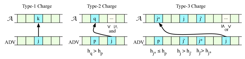
Figure 3: Four types of charges. The vertical inequality signs between the schedules show the relation between the temperatures.

We now describe this charging scheme. (See Figure 3 for illustration.) There will be three types of charges, depending on whether ${\cal A}$ is busy or idle at a given time step and on the relative temperatures of the schedules of ${\cal A}$ and the adversary. The temperature at time $u$ in the schedules of ${\cal A}$ and the adversary will be denoted by $\tau_{u}$ and $\tau^{\prime}_{u}$, respectively.

Suppose that at some time $u$, ${\cal A}$ schedules a job $k$ while the adversary schedules a job $j$, or that the adversary is idle (we treat this case as if executing a job $j$ with $h_{j}=0$.) Then step $u$ will be called a relative-heating step if $k$ is strictly hotter than $j$, that is $h_{k}>h_{j}$. Note that if $\tau_{v}>\tau^{\prime}_{v}$ for some time $v$, then a relative-heating step must have occurred before time $v$.

Consider now a job $j$ scheduled by the adversary, say at time $v$. The charge of $j$ is defined as follows:

Type 1 Charges: If ${\cal A}$ schedules a job $k$ at time $v$, charge $j$ to $k$. Otherwise, we are idle, and then we have two more cases.

Type-2 Charges: Suppose that ${\cal A}$ is hotter than the adversary at time $v$ but not at $v+1$, that is $\tau_{u}>\tau^{\prime}_{u}$ and $\tau_{u+1}\leq\tau^{\prime}_{u+1}$. In this case we charge $j$ to the job $q$ executed by ${\cal A}$ in the last relative-heating step before $v$. (As explained above, this step exists.)

Type-3 Charges: Suppose now that either ${\cal A}$ is not hotter than the adversary at $v$ or ${\cal A}$ is hotter than the adversary at $v+1$. In other words, $\tau_{v}\leq\tau^{\prime}_{v}$ or $\tau_{v+1}>\tau^{\prime}_{v+1}$. (Note that in the latter case we must also have $\tau_{v}>\tau^{\prime}_{v}$ as well, since the algorithm is idle.)

We claim that $\tau_{v}+h_{j}\leq 2$, which means that neither $j$ or any job $\ell$ with $h_{\ell}\leq h_{j}$ can be pending at $v$. To justify this, we consider the two sub-cases of the condition for type-3 charges. If $\tau_{v}\leq\tau^{\prime}_{v}$, the claim is trivial, since then $\tau_{v}+h_{j}\leq\tau^{\prime}_{v}+h_{j}\leq 2$, because the adversary executes $j$ at time $v$. So assume now that $\tau_{v+1}>\tau^{\prime}_{v+1}$. Since ${\cal A}$ is idle, we have $\tau_{v+1}\leq 1/2$. Therefore $h_{j}=2\tau^{\prime}_{v+1}-\tau^{\prime}_{v}\leq 2\tau^{\prime}_{v+1}\leq 1$, and the claim follows because $\tau_{v}\leq 1$ as well.

From the above claim, $j$ was scheduled by ${\cal A}$ at some time $u<v$. To find a job that we can charge $j$ to, we construct a chain of jobs $j,j^{\prime},j^{\prime\prime},\ldots,j^{\ast}$ with strictly decreasing heat contributions. Further, all jobs in this chain except $j^{\ast}$ will be executed by ${\cal A}$ at relative-heating steps. This chain will be determined uniquely by $j$, and we will charge $j$ to $j^{\ast}$. If, at time $u$, the adversary is idle or schedules an equal or hotter job, then $j^{\ast}=j$, that is, we charge $j$ to itself (its “copy” in ${\cal A}$’s schedule). Otherwise, if the adversary schedules $j^{\prime}$ at time $u$ then $j^{\prime}$ is strictly cooler than $j$, that is $h_{j^{\prime}}<h_{j}$. Now we claim that the algorithm schedules $j^{\prime}$ at some time before $v$. Indeed, if $j^{\prime}$ is scheduled before $u$, we are done. Otherwise, $j^{\prime}$ is pending at $u$, and, since the algorithm never schedules a dominated job, we must have $d_{j^{\prime}}\geq d_{j}\geq v+1$. By our earlier observation and by $h_{j^{\prime}}<h_{j}$, if ${\cal A}$ did not schedule $j^{\prime}$ before $v$, then $j^{\prime}$ would have been admissible at $v$, contradicting the fact ${\cal A}$ is idle at $v$. So now the chain is $j,j^{\prime}$. Let $u^{\prime}$ be the time when ${\cal A}$ schedules $j^{\prime}$. If the adversary is idle at time $u^{\prime}$ or if $j^{\prime}$ is not hotter than the job executed by the adversary at time $u^{\prime}$, we take $j^{\ast}=j^{\prime}$. Otherwise, we take $j^{\prime\prime}$ to be the job executed by the adversary at time $u^{\prime}$, and so on. This process must end at some point, since we deal with strictly cooler and cooler jobs. So the job $j^{\ast}$ is well-defined.

This completes the description of the charging scheme. Now we show that any job scheduled by ${\cal A}$ will get at most two charges. Obviously, each job in ${\cal A}$’s schedule gets at most one type-1 charge. In-between any two time steps that satisfy the condition of the type-2 charge there must be a relative-heating step, so the type-2 charges are assigned to distinct relative-heating steps. As for type-3 charges, every chain defining a type-3 charge is uniquely defined by the first considered job, and these chains are disjoint. Therefore type-3 charges are assigned to distinct jobs.

Now let $k$ be a job scheduled by ${\cal A}$ at some time $v$. By the previous paragraph, $k$ can get at most one charge of each type. We claim that $k$ cannot get charges of each type $1$, $2$ and $3$. Indeed, if $k$ receives a type-1 charge, then the adversary is not idle at time $v$, and schedules some job $\ell$. If $k$ also receives a type-2 charge, then $v$ must be a relative-heating step, that is $h_{k}>h_{\ell}$. But to receive a type-3 charge, $k$ would be the last job $j^{\ast}$ in a chain of some job $j$, and since the chain was not extended further, we must have $h_{k}\leq h_{\ell}$. So type-1, type-2 and type-3 charges cannot coincide.

Summarizing the argument, we have that every job scheduled by the adversary is charged to some job scheduled by ${\cal A}$, and every job scheduled by ${\cal A}$ receives no more than $2$ charges. Therefore the competitive ratio of ${\cal A}$ is not more than $2$. $\Box$

5 A Lower Bound on the Competitive Ratio

Theorem 4

Every deterministic online algorithm for $1|\textrm{online-}r_{i},h_{i},p_{i}=1|\sum U_{i}$ has competitive ratio at least $2$.

Proof: Fix some deterministic online algorithm ${\cal A}$. We (the adversary) release a job $1\to(0,3,1.2)$ (in notation $j\to(r_{j},d_{j},h_{j})$). If ${\cal A}$ schedules it at time $0$, we release at time $1$ a tight job $2\to(1,2,1.6)$ and schedule it followed by $1$. ${\cal A}$’s schedule is too hot at time $1$ to execute job $2$. If ${\cal A}$ does not schedule job $1$ at time $0$, then we schedule it at $0$ and release at time $2$ (and schedule) a tight job $3\to(2,3,1.6)$ at time $2$. In this case, ${\cal A}$ cannot complete both jobs $1$ and $3$ without violating the thermal threshold. In both cases we schedule two jobs, while ${\cal A}$ schedules only one, completing the proof. (See Figure 4.) $\Box$

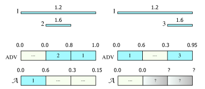
Figure 4: The lower bound for deterministic algorithms.

6 Final Comments

Many open problems remain. Perhaps the most intriguing one is to determine the randomized competitive ratio for the problem we studied. The proof of Theorem 4 can easily be adapted to prove the lower bound of $1.5$, but we have not been able to improve the upper bound of $2$; this is, in fact, the main focus of our current work on this scheduling problem. One approach, based on Theorem 3, would be to randomly choose, at the beginning of computation, two different reasonable algorithms ${\cal A}_{1}$, ${\cal A}_{2}$, each with probability $1/2$, and then deterministically execute the chosen ${\cal A}_{i}$. So far, we have been able to show that for many natural choices for ${\cal A}_{1}$ and ${\cal A}_{2}$ (say, CoolestFirst and EarliestDeadlineFirst), this approach does not work.

Extensions of the cooling model can be considered, where the temperature after executing $j$ is $(\tau+h_{j})/R$, for some $R>1$. Even this formula, however, is only a discrete approximation for the true model (see, for example, [11]), and it would be interesting to see if the ideas behind our $2$-competitive algorithm can be adapted to these more realistic cases.

In reality, thermal violations do not cause the system to idle, but only to reduce the frequency. With frequency reduced to half, a unit job will execute for two time slots. Several frequency levels may be available.

We assumed that the heat contributions are known. This is counter-intuitive, but not unrealistic, since the ”jobs” in our model are unit slices of longer jobs. Prediction methods are available that can quite accurately predict the heat contribution of each slice based on the heat contributions of the previous slices. Nevertheless, it may be interesting to study a model where exact heat contributions are not known.

Other types of jobs may be studied. For real-time jobs, one can consider the case when not all jobs are equally important, which can be modeled by assigning weights to jobs and maximizing the weighted throughput. For batch jobs, other objective functions can be optimized, for example the flow time.

One more realistic scenario would be to represent the whole processes as jobs, rather then their slices. This naturally leads to scheduling problems with preemption and with jobs of arbitrary processing times. When the thermal threshold is reached, the execution of a job is slowed down by a factor of $2$. Here, a scheduling algorithm may decide to preempt a job when another one is released or, say, when the processor gets too hot.

Finally, in multi-core systems one can explore the migrations (say, moving jobs from hotter to cooler cores) to keep the temperature under control. This leads to even more scheduling problems that may be worth to study.

References

- [1] F. Bellosa, A. Weissel, M. Waitz, and S. Kellner. Event-driven energy accounting for dynamic thermal management. In Workshop on Compilers and Operating Systems for Low Power, 2003.
- [2] J. Choi, C-Y. Cher, H. Franke, H. Hamann, A. Weger, and P. Bose. Thermal-aware task scheduling at the system software level. In International Symposium on Low Power Electronics and Design,, pages 213–218, 2007.
- [3] M.R. Garey and D.S. Johnson. Computers and Intractability: A Guide to the Theory of NP-Completeness. W.H.Freeman and Co., 1979.
- [4] M. Gomaa, M. D. Powell, and T. N. Vijaykumar. Heat-and-run: leveraging smt and cmp to manage power density through the operating system. SIGPLAN Not., 39(11):260–270, 2004.
- [5] S. Irani and K. R. Pruhs. Algorithmic problems in power management. SIGACT News, 36(2):63–76, 2005.
- [6] M. Martonosi J. Donald. Techniques for multicore thermal management: Classification and new exploration. In Proceedings of the International Symposium on Computer Architecture, pages 78–88, 2006.
- [7] A. Kumar, L. Shang, L-S. Peh, and N. K. Jha. HybDTM: a coordinated hardware-software approach for dynamic thermal management. In DAC ’06: Proceedings of the 43rd Annual Conference on Design Automation, pages 548–553, 2006.
- [8] E. Kursun, C.-Y. Cher, A. Buyuktosunoglu, and P. Bose. Investigating the effects of task scheduling on thermal behavior. In the 3rd Workshop on Temperature-Aware Computer Systems, 2006.
- [9] A. Merkel and F. Bellosa. Balancing power consumption in multiprocessor systems. SIGOPS Oper. Syst. Rev., 40(4):403–414, 2006.
- [10] J. Moore, J. Chase, P. Ranganathan, and R. Sharma. Making scheduling ”cool”: temperature-aware workload placement in data centers. In ATEC’05: Proceedings of the USENIX Annual Technical Conference 2005 on USENIX Annual Technical Conference, pages 5–5, 2005.
- [11] J. Yang, X. Zhou, M. Chrobak, and Y. Zhang. Dynamic thermal management through task scheduling. In IEEE International Symposium on Performance Analysis of Systems and Software, 2008. To appear.