Introduction to the Pinch Technique

Abstract

These notes are a short introduction to the pinch technique. We present the one-loop calculations for basic QCD Green’s functions. The equivalence between the pinch technique and the background field method is explicitly shown at the one-loop level. We review the absorptive pinch technique in the last sections. These lectures are a compilation of relevant papers on this subject and are prepared for the third Modave Summer School in Mathematical Physics.

1 Introduction

When quantizing gauge theories in the continuum one must invariably resort to an appropriate gauge-fixing procedure in order to remove redundant (non-dynamical) degrees of freedom originating from the gauge invariance of the theory. Thus, one adds to the gauge invariant (classical) Lagrangian ${\cal L}_{\rm I}$ a gauge-fixing term ${\cal L}_{\rm GF}$, which allows for the consistent derivation of Feynman rules. At this point a new type of redundancy makes its appearance, this time at the level of the building blocks defining the perturbative expansion. In particular, individual off-shell Green’s functions ($n$-point functions) carry a great deal of unphysical information, which disappears when physical observables are formed. $S$-matrix elements, for example, are independent of the gauge-fixing scheme and parameters chosen to quantize the theory, they are gauge-invariant (in the sense of current conservation), they are unitary (in the sense of conservation of probability), and well behaved at high energies. On the other hand Green’s functions depend explicitly (and generally non-trivially) on the gauge-fixing parameter entering in the definition of ${\cal L}_{\rm GF}$, they grow much faster than physical amplitudes at high energies (e.g. they grossly violate the Froissart-Martin bound [3]), and display unphysical thresholds. Last but not least, in the context of the standard path-integral quantization by means of the Faddeev-Popov Ansatz, Green’s functions satisfy complicated Slavnov-Taylor identities [4] involving ghost fields, instead of the usual Ward identities generally associated with the original gauge invariance.

The above observations imply that in going from unphysical Green’s functions to physical amplitudes, subtle field theoretical mechanisms are at work, implementing vast cancellations among the various Green’s functions. Interestingly, these cancellations may be exploited in a very particular way by the Pinch Technique (PT) [5, 6, 7, 8]: A given physical amplitude is reorganized into sub-amplitudes, which have the same kinematic properties as conventional $n$-point functions (self-energies, vertices, boxes) but, in addition, they are endowed with important physical properties. This has been accomplished diagrammatically, at the one- and two-loop level, by recognizing that longitudinal momenta circulating inside vertex and box diagrams generate, by “pinching” out internal fermion lines, propagator-like terms. The latter are reassigned to conventional self-energy graphs in order to give rise to effective Green’s functions which manifestly reflect the properties generally associated with physical observables. In particular, the PT Green’s function are independent of the gauge-fixing scheme and parameters chosen to quantize the theory ($\xi$ in covariant gauges, $n_{\mu}$ in axial gauges, etc.), they are gauge-invariant, i.e., they satisfy simple tree-level-like Ward identities associated with the gauge symmetry of the classical Lagrangian ${\cal L}_{\rm I}$, they display only physical thresholds, and, finally, they are well behaved at high energies.

Given the subtle nature of the problem, the question naturally arises, what set of physical criteria must be satisfied by a resummation algorithm, in order for it to qualify as “physical”. In other words, what are the guiding principles, which will allow one to determine whether or not the resumed quantity carries any physically meaningful information, and to what extend it captures the essential underlying dynamics? To address these questions in this notes, we postulate a set of field-theoretical requirements that we consider crucial when attempting to define a proper resumed propagator. Our considerations propose an answer to the question of how to analytically continue the Lehmann–Symanzik–Zimmermann formalism [9] in the off-shell region of Green’s functions in a way which is manifestly gauge-invariant and consistent with unitarity. In addition, we demonstrate that the off-shell Green’s functions obtained by the pinch technique satisfy all these requirements. In fact, these requirements are, in a way, inherent within the PT approach, as we will see in detail in what follows.

In particular, the following is required from an off-shell, one-particle irreducible (1PI), effective two-point function:

• Resummability. The effective two-point functions must be resummable. For the conventionally defined two-point functions, the resummability can be formally derived from the path integral. In the $S$-matrix PT approach, the resummability of the effective two-point functions is more involved and must be based on a careful analysis of the structure of the $S$-matrix to higher orders in perturbation theory [10].

• Analyticity of the off-shell Green’s function. An analytic two-point function has the property that its real and imaginary parts are related by a dispersion relation (DR), up to a maximum number of two subtractions. The latter is a necessary condition when considering renormalizable Green’s functions, as we will discuss in Sec. 6.

• Unitarity and the optical relation. In the conventional framework, unitarity is defined only for on-shell $S$-matrix elements, leading to the familiar optical theorem (OT) for the forward scattering. Here, we postulate the validity of the optical relation for the off-shell Green’s function, when embedded in an $S$-matrix element, in a way which will become clear in what follows. An important consequence of this requirement is that the imaginary part of the off-shell Green’s function should not contain any unphysical thresholds. As a counter-example, it is shown in [11] that this pathology is in fact induced by the quantum fields in the background-field-gauge (BFG) method [12, 13, 14, 16] for $\xi_{Q}\not=1$.

• Gauge invariance. As has been mentioned above, one has to require that the effective Green’s functions are gauge-fixing parameter (GFP) independent and satisfy Ward identities in compliance with the classical action. For instance, the latter is guaranteed in the BFG method but not the former. This condition also guarantees that gauge invariance does not get spoiled after Dyson summation of the GFP-independent self-energies. In some of the recent literature, the terms of gauge invariance and gauge independence have been used for two different aspects. For example, in the BFG the classical background fields respect gauge invariance in the classical action. However, this fact does not ensure that the quantum fields respect some form of quantum gauge invariance, neither does imply that some kind of a Becchi-Rouet-Stora (BRS) symmetry [17] is present for the fields inside the quantum loops after fixing the gauge of the theory [18, 19]. In our discussion, when referring to gauge invariance, we will encompass both meanings, i.e., gauge invariance of the tree-level classical particles as well as BRS invariance of the quantum fields. A direct but non-trivial consequence of the gauge invariance and of the abelian-type Ward identitites that the effective off-shell Green’s functions satisfy is that for large asymptotic momenta transfers ($s\to\infty$), the self-energy under construction must capture the running of the gauge coupling, as it happens in Quantum ElectroDynamics (QED). Because of the abelian-type WIs and on account of resummation, the above argument can be generalized to $n$-point functions. In addition, the off-shell $n$-point transition amplitudes should display the correct high-energy limit as is dictated by the Equivalence Theorem [20].

• Multiplicative renormalization. Since we are interested in renormalizable theories, i.e., theories containing operators of dimension no higher than four, the off-shell Green’s functions calculated within an approach should admit renormalization. However, this requirement alone is not sufficient when resummation is considered. The appearance of a two-point function in the denominator of a resummed propagator makes it unavoidable to demand that renormalization be multiplicative. Otherwise, the analytic expressions will suffer from spurious ultraviolet (UV) divergences. Particular examples of the kind are some ghost-free gauges, such as the light-cone or planar gauge [21].

• Position of the pole. Since the position of the pole is the only gauge-invariant quantity that one can extract from conventional self-energies, any acceptable resummation procedure should give rise to effective self-energies which do not shift the position of the pole. This requirement drastically reduces the arbitrariness in constructing effective two-point correlation function.

The first question one may wonder in this context is about the conceptual and phenomenological advantages of being able to work with such special Green’s functions. We briefly discuss here some concept where the pinch technique was used.

• QCD effective charge: The unambiguous extension of the concept of the gauge-independent, renormalization group invariant, and process independent [22] effective charge from QED to QCD [23, 5], is of special interest for several reasons [24]. The PT construction of this quantity accomplishes the explicit identification of the conformally-(in)variant subsets of QCD graphs [25], usually assumed in the field of renormalon calculus [26].

• Breit-Wigner resummations, resonant transition amplitudes, unstable particles: The Breit-Wigner procedure used for regulating the physical singularity appearing in the vicinity of resonances ($\sqrt{s}\sim M$) is equivalent to a reorganization of the perturbative series [27]. In particular, the Dyson summation of the self-energy $\Pi(s)$ amounts to removing a particular piece from each order of the perturbative expansion, since from all the Feynman graphs contributing to a given order $n$ one only picks the part which contains $n$ self-energy bubbles $\Pi(s)$, and then one takes $n\to\infty$. Given that non-trivial cancellations involving the various Green’s function is generally taking place at any given order of the conventional perturbative expansion, the act of removing one of them from each order may distort those cancellations, this is indeed what happens when constructing non-Abelian running widths. The pinch technique ensures that all unphysical contributions contained inside $\Pi(s)$ have been identified and properly discarded, before $\Pi(s)$ undergoes resummation [10, 28].

• Off-shell form-factors: In non-Abelian theories, their proper definition poses in general problems related to the gauge invariance [29]. Some representative cases have been the magnetic dipole and electric quadrupole moments of the $W$ [30], the top-quark magnetic moment [31], and the neutrino charge radius [32]. The pinch technique allows for an unambiguous definition of such quantities. Most notably, the gauge-independent, renormalization-group- invariant, and target-independent neutrino charge radius constitutes a genuine physical observable, since it can be extracted (at least in principle) from experiments [33].

• Schwinger-Dyson equations: This infinite system of coupled non-linear integral equations for all Green’s functions of the theory is inherently non-perturbative and can accommodate phenomena such as chiral symmetry breaking and dynamical mass generation. In practice one is severely limited in their use, and a self-consistent truncation scheme is needed. The main problem in this context is that the Schwinger-Dyson equations are built out of gauge-dependent Green’s functions. Since the cancellation mechanism is very subtle, involving a delicate conspiracy of terms from all orders, a casual truncation often gives rise to gauge-dependent approximations for ostensibly gauge-independent quantities [34, 35]. The role of the pinch technique in this problem is to trade the conventional Schwinger-Dyson series for another, written in terms of the new, gauge-independent building blocks [5, 36, 37]. The upshot of this program is then to truncate this new series, by keeping only a few terms in a “dressed-loop” expansion, and maintain exact gauge-invariance, while at the same time accommodating non-perturbative effects. Further explanations of this non perturbative pinch technique can be found in [38].

• Other interesting applications include the gauge-invariant formulation of the $\rho$ parameter at one-[39] and two-loops [40], various finite temperature calculations [41], a novel approach to the comparison of electroweak data with theory [42], resonant CP violation [43], the construction of the two-loop PT quark self-energy [44], and more recently the issue of particle mixings [45].

The algorithms of the S-matrix and the intrinsic pinch technique, presented in these notes, allow us to extract Green’s functions with appropriate physical properties. These algorithms are easily perform at the one-loop level. Nevertheless, even though the generalisation up to an arbitrary number of loop is straightforward, the calculation become quickly tedious. Fortunately, a correspondence between the PT and the background field method was found and allow us to apply directly the Feynman rules of the latter to obtain the same Green’s functions.

The Background Field Method (BFM) was first introduced by DeWitt [12] as a technique for quantizing gauge field theories while retaining explicit gauge invariance. In its original formulation, DeWitt worked only for one-loop calculations. The multi-loop extension of the method was given by ’t Hooft [13], DeWitt [14], Boulware [15], and Abbott [16]. Using these extensions of the background field method, explicit two-loop calculations of the $\beta$ function for pure Yang-Mills theory was made first in the Feynman gauge [16, 46], and later in the general gauge [47].

Both pinch technique and background field method have the same interesting feature. The Green’s functions (gluon self-energies, proper gluon-vertices, etc.) constructed by the two methods retain the explicit gauge invariance, thus obey the naive Ward identities. As a result, for example, a computation of the QCD $\beta$-function coefficient is much simplified. The only thing we need to do is to construct the gauge-invariant gluon self-energy in either method and to examine its ultraviolet-divergent part. Either method gives the same correct answer [6, 16]. The connection between the background field method and the pinch technique was first established for the one- [48] and two-loop [49] levels. The extension of the pinch technique to all orders for QCD was carried out and the connection was shown to persist also to all orders in [50]. This connection also hold in the electroweak sector where the PT construction to all orders was performed in [51].

These notes are a compilation of many papers on this subject. We refer the interested readers to these references for further developments. We present in these lectures notes two versions of the pinch technique for a Yang-Mills theory. The S-matrix pinch technique and the intrinsic pinch technique are explain in Sec. 2 on the example of the gluon self-energy. We review the background field method in Sec. 3 where the equivalence of the BFM and the conventional effective actions is proved. We show also that the BFM gluon self-energy correspond to the PT gluon self-energy at the one-loop level. In Sec. 4, we develop the construction on the gauge-invariant proper 3-gluon vertex by the intrinsic pinch technique and the background field method, and we give the Ward identity satisfied by this proper vertex. The Ward identity satisfied by the gauge-invariant 4-gluon vertex is also presented. Some basic concepts of quantum field and their implications are reviewed in Sec. 5. The absorptive pinch technique construction is presented in Sec. 6. The first appendix is devoted to Ward and Slanov-Taylor identities. Finally, a short development with the dimensional regularization and the Feynman rules are relegated to the appendix B and C.

2 The Pinch Technique

2.1 The S-matrix pinch technique

The gluon self-energy is the simplest example that demonstrate how the pinch technique works. We define the gluon self-energy $i\Pi_{\mu\nu}$ as the sum of all one particle irreducible diagrams with two gluon legs. The one loop contributions are

(2.1)

This self-energy is transverse thanks to the Ward identity (see Appendix A), like in QED, and can be written

$$\Pi_{\mu\nu}(q)=t_{\mu\nu}(q)\Pi(q^{2}),$$ (2.2)

with the transverse projector $t_{\mu\nu}(q)=g_{\mu\nu}-q_{\mu}q_{\nu}q^{-2}$. This implies that the gluon remains massless at any order in perturbation theory and also that $\Pi$ can be renormalized with only one renormalization factor. A straightforward calculation shows the this conventional (renormalized) gluon self-energy, written here at the one-loop level with $n_{f}$ flavours of massless fermion

$$\Pi(q^{2})=\frac{g^{2}q^{2}}{16\pi^{2}}\left\{\left[\left(-\frac{13}{6}+\frac{\xi}{2}\right)N+\frac{2}{3}n_{f}\right]\ln(\frac{q^{2}}{\mu^{2}})+\left(\frac{97}{36}+\frac{\xi}{2}+\frac{\xi^{2}}{4}\right)N-\frac{10}{9}n_{f}\right\},$$ (2.3)

depends on the gauge-fixing parameter $\xi$, in the Lorentz covariant gauges, defined by the free gluon propagator

$$\Delta_{\mu\nu}^{(0)}(q)=\frac{-i}{q^{2}}\left[g_{\mu\nu}-(1-\xi)\frac{q_{\mu}q_{\nu}}{q^{2}}\right].$$ (2.4)

Resuming all one-particle irreducible graphs, the full gluon two-point function reads

$$\Delta_{\mu\nu}=-i\left[t_{\mu\nu}(q)\Delta(q^{2})+\xi\frac{q_{\mu}q_{\nu}}{q^{4}}\right],\quad\text{where }\quad\Delta(q^{2})=\frac{1}{q^{2}-\Pi(q^{2})}.$$ (2.5)

Note that the dressed propagator depends on the gauge-fixing parameter on a trivial way, given by the tree level propagator (see Appendix A), but also through the self-energy. Although it is possible to sum the renormalized gluon self-energy in a Dyson series to give a radiatively corrected gluon propagator, the quantity defined by analogy with the QED effective charge is in general gauge-, scale- and scheme-dependent, and at asymptotic $q^{2}$ does not match on to the QCD running coupling defined from the renormalization group. The interested readers may find more information on the gauge-invariant QCD effective charge in [24]. Let us mention also that in axial gauges, the gluon propagator is not multiplicatively renormalizable [5].

Others pathologies of conventional Green’s functions can be seen on the example on the Higgs-boson self-energy [28]. At the one loop level, the $W$ corrections,

leads to a Higgs self-energy,

$$\begin{split}\Pi_{H}=\frac{\alpha_{W}}{4\pi}\bigg{[}&\left(\frac{(q^{2})^{2}}{4M_{W}^{2}}-q^{2}+3M_{W}^{2}\right)B_{0}(q^{2},M_{W}^{2},M_{W}^{2})\\ &+\frac{M_{H}^{4}-(q^{2})^{2}}{4M_{W}^{2}}B_{0}(q^{2},\xi_{W}M_{W}^{2},\xi_{W}M_{W}^{2})\bigg{]},\end{split}$$ (2.6)

with

$$B_{0}(q^{2},m_{1}^{2},m_{2}^{2})=(2\pi\mu)^{4-d}\int\frac{d^{d}k}{i\pi^{2}}\frac{1}{(k^{2}-m_{1}^{2})[(k+q)^{2}-m_{2}^{2}]},$$ (2.7)

which clearly develops unphysical threshold, i.e. $\xi_{W}$-dependent threshold. Moreover the $(q^{2})^{2}$ term violates the Froissard-Martin bound (see Sec.5). As explained in [28], these pathologies disappear after the pinch technique has been carried out.

In QED the photon self-energy (also called the vacuum polarisation tensor) is easily computed at the one loop level,

$$\Pi_{\text{QED}}^{(1)}(q^{2})=\frac{\alpha}{3\pi}q^{2}\left[\ln\left(\frac{q^{2}}{m^{2}}\right)-\frac{5}{3}\right],$$ (2.8)

since the only diagram is a fermion loop. $m$ is the electron mass and we used the on-shell regularization scheme. This expression show us that, first, the photon remains massless and, secondly, the strength of the interaction increases with the Euclidean momentum $q^{2}$. The modification of the photon propagator induced by a fermion loop can be absorbed in the definition of the fine structure

$$\alpha(q^{2})=\frac{\alpha}{1-(\alpha/3\pi)\ln(q^{2}/Am^{2})},$$ (2.9)

with $A=\exp(5/3)$. As we will see, it is also possible to define an effective charge gauge-independent for QCD.

We now review the S-matrix pinch technique as it applies to the effective propagator. The idea is to begin with something we know to be gauge invariant, the S-matrix, and extract from this the corresponding gauge-invariant Green’s function. Note that it is the proper self-energy will be gauge invariant, the propagator has a trivial gauge dependence through the free propagator and this induces an equally trivial dependence in the two-points Green’s function.

Consider the S-matrix element T for the elastic scattering of two fermions of masses $m_{1}$ and $m_{2}$. By asymptotic freedom, perturbation theory is relevant for large momenta, i.e. in the ultra-violet region, the quarks are free states and satisfy the Dirac equation $(p\!\!\!/-m)u(p)=iS^{-1}(p)u(p)=0$. To any order in perturbation theory, T is independent of the gauge-fixing parameter $\xi$ [52]. But, as an explicit calculation shows, the conventionally defined proper self-energy at the one-loop level depends on $\xi$. At the one-loop level, this dependence is cancelled by contributions from other graphs, such as (e), (f) and (g) in Fig. 1, which, at first glance, do not seem to be propagator-like. Note that the graphs (f) and (g) have a mirror counterpart and the graph (e) has a crossed counterpart not shown in Fig. 1. That this cancelation must occur and can be employed to defined a gauge-invariant self-energy, is evident from the decomposition

$$T(s,t,m_{1},m_{2})=T_{1}(t,\xi)+T_{2}(t,m_{1},m_{2},\xi)+T_{3}(s,t,m_{1},m_{2},\xi),$$ (2.10)

where the function $T_{1}(t)$ depends only on the Mandelstram variable $t=-(p^{\prime}_{1}-p_{1})^{2}=-q^{2}$, and not on $s=(p_{1}+p_{2})^{2}$ or on the external masses. Typically, self-energy, vertex, and box diagrams contribute to $T_{1}$, $T_{2}$ and $T_{3}$, respectively. Moreover, such contributions are $\xi$ dependent. However, as the sum $T(s,t,m_{1},m_{2})$ is gauge invariant, it is easy to show that Eq. (2.10) can be recast in the form

$$T(s,t,m_{1},m_{2})=\hat{T}_{1}(t)+\hat{T}_{2}(t,m_{1},m_{2})+\hat{T}_{3}(s,t,m_{1},m_{2}),$$ (2.11)

where the $\hat{T}_{i}\ (i=1,2,3)$ are separately $\xi$ independent. To proof this assertion we derive Eq. (2.10) to obtain $\partial^{2}T_{3}/\partial s\partial\xi=0$. Hence $T_{3}$ can be written as

$$T_{3}(s,t,m_{1},m_{2},\xi)=\hat{T}_{3}(s,t,m_{1},m_{2})+T^{\prime}_{3}(t,m_{1},m_{2},\xi).$$ (2.12)

The part $T^{\prime}_{3}$ is added to $T_{2}$ and we can iterate this process to obtain the decomposition (2.11).

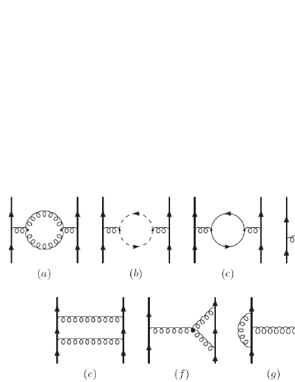
Figure 1: Fermions scattering at order $g^{4}$

.

.5 The propagator-like parts of graphs such as Fig. 7, which enforce the gauge independence of $T_{1}(t)$, are called “pinch parts”. The pinch part emerge every time a gluon propagator or an elementary three-gluon vertex contribute a longitudinal momentum $k_{\mu}$ to the original graph’s numerator. The action of such a term is to trigger an elementary Ward identity of the form

$$k^{\mu}\gamma_{\mu}\equiv k\!\!\!/ = (p\!\!\!/+k\!\!\!/-m)-(p\!\!\!/-m),$$ (2.13)

$$= iS^{-1}(p+k)-iS^{-1}(p),$$

once it gets contracted with a $\gamma$ matrix. The first term on the right-hand side of Eq. (2.13) will remove the internal fermion propagator, that is a “pinch”, whereas $S^{-1}(p)$ vanish on shell.

Returning to the decomposition of Eq.(2.10), the function $\hat{T}_{1}$ is gauge invariant and may be identified with the contribution of the new propagator. We can construct the new propagator, or equivalently $\hat{T}_{1}$, directly from the Feynman rules. In doing so it is evident that any value for the gauge parameter $\xi$ may be chosen, since $\hat{T}_{1}$, $\hat{T}_{2}$ and $\hat{T}_{3}$ are all independent of $\xi$. The simplest of covariant gauges is certainly the Feynman gauge ($\xi=1$), which removes the longitudinal part of the gluon propagator. Therefore the only possibility for pinching in four-fermions amplitudes arises from the momentum of the three-gluon vertices, and the only propagator-like contributions come from graph of Fig. 2 (and its mirror counterpart).

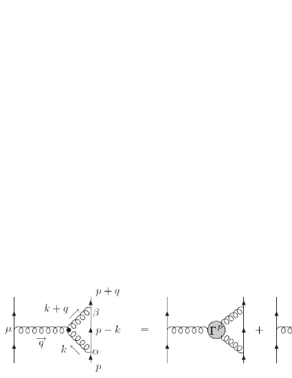
Figure 2: Decomposition of the vertex diagram in its pinch and regular parts.

The amplitude of this diagram ($\bm{T}_{a}$ are the generators of the gauge group)

$$\bar{u}_{1}(ig\bm{T}_{a})\gamma^{\mu}u_{1}\frac{(-i)}{q^{2}}gf^{abc}\int\frac{d^{4}k}{(2\pi)^{4}}\frac{\Gamma_{\alpha\mu\beta}(k,q)}{k^{2}(k+q)^{2}}\bar{u}_{2}(ig\bm{T}_{b})\gamma^{\alpha}S(p-k)(ig\bm{T}_{c})\gamma^{\beta}u_{2}$$ (2.14)

has a pinch part $i\Pi_{\mu\nu}^{P}$ who belongs to $\hat{T}_{1}(t)$ of the form

$$[\bar{u}_{1}(ig\bm{T}_{a})\gamma^{\mu}u_{1}]\frac{(-i)}{q^{2}}\ i\Pi^{P}_{\mu\nu}\delta^{ab}\ \frac{(-i)}{q^{2}}[\bar{u}_{2}(ig\bm{T}_{b})\gamma^{\nu}u_{2}].$$ (2.15)

The correct color factor is recover by using the antisymmetry of the structure constants

$$2f^{abc}\bm{T}_{b}\bm{T}_{c}=f^{abc}\left[\bm{T}_{b},\bm{T}_{c}\right]=if^{abc}f^{bcd}\bm{T}_{d}=iN\delta^{ad}\bm{T}_{d}.$$ (2.16)

This relation is valid for any representation $\bm{T}^{a}$ of the Lie algebra $\mathfrak{su}(N)$ where $N$ is the color number. If we take the adjoint representation $(\bm{T}^{a})^{bc}=-if^{abc}$, we get another relation

$$2f^{axy}f^{bxz}f^{cyz}=Nf^{abc},$$ (2.17)

useful when dealing with the 4-gluon vertex. To explicit calculate the pinching contribution of the graph of Fig. 2, it is convenient to decompose the vertices into two pieces. A piece $\Gamma^{F}$ which has terms with external momentum $q$ and a piece $\Gamma^{P}$ which carries the internal momentum only:

$$\Gamma_{\alpha\mu\beta}(k,q) = (k-q)_{\beta}g_{\alpha\mu}+(k+2q)_{\alpha}g_{\mu\beta}-(2k+q)_{\mu}g_{\beta\alpha}$$

$$= \Gamma_{\alpha\mu\beta}^{F}(k,q)+\Gamma_{\alpha\mu\beta}^{P}(k,q)$$

$$\Gamma_{\alpha\mu\beta}^{F}(k,q) = -(2k+q)_{\mu}g_{\alpha\beta}+2q_{\alpha}g_{\mu\beta}-2q_{\beta}g_{\mu\alpha}$$

$$\Gamma_{\alpha\mu\beta}^{P}(k,q) = k_{\alpha}g_{\mu\beta}+(k+q)_{\beta}g_{\alpha\mu}$$

Now $\Gamma^{F}_{\mu\nu\alpha}$ satisfies a Feynman-gauge Ward identity:

$$q^{\mu}\Gamma^{F}_{\alpha\mu\beta}=[k^{2}-(k+q)^{2}]g_{\alpha\beta},$$ (2.19)

where the Right Hand Side (RHS) is the difference of two inverse propagators in the Feynman gauge. As for $\Gamma^{P}_{\mu\nu\alpha}$, it gives rise to pinch parts when contracted with $\gamma$ matrices

$$g_{\mu\alpha}(q\!\!\!/+k\!\!\!/) = ig_{\mu\alpha}[S^{-1}(p+q)-S^{-1}(p-k)],$$

$$g_{\nu\alpha}k\!\!\!/ = ig_{\nu\alpha}[S^{-1}(p)-S^{-1}(p-k)].$$ (2.20)

Both $S^{-1}(p+q)$ and $S^{-1}(p)$ vanish on shell, whereas the two terms proportional to $S^{-1}(p-k)$ pinch out the internal fermion propagator in graph of Fig. 2, and so we are left with two “pinch” (propagator-like) parts and one “regular” (purely vertex-like) part, namely

$$= i\Pi_{\mu\nu}^{P}\gamma^{\mu}$$ (2.21)

$$= Ng^{2}\int\frac{d^{4}k}{(2\pi)^{4}}\frac{1}{k^{2}(k+q)^{2}}(g_{\mu\nu}\gamma^{\nu})$$

regular part $$= \frac{1}{2}Ng^{2}\int\frac{d^{4}k}{(2\pi)^{4}}\frac{\gamma^{\rho}S(p-k)\gamma^{\sigma}}{k^{2}(k+q)^{2}}{\Gamma}^{F}_{\rho\sigma\mu}$$ (2.22)

We can always add a $q_{\mu}$ term in the expression of the pinch part since this term vanishes when contracted with the conserved current of the quark $\bar{u}(p)\gamma^{\mu}u(p+q)$. The cancellation with the self-energy is more evident if we write the total pinch contribution of the vertex-like diagrams

$$\boxed{i\Pi^{P}_{\mu\nu}(q)=2Ng^{2}q^{2}t_{\mu\nu}(q)\int\frac{d^{4}k}{(2\pi)^{4}}\frac{1}{k^{2}(k+q)^{2}}}$$ (2.23)

A factor two comes from the mirror contribution and the $q^{2}$ is added to recover the expression (2.15). This multiplicative factor $q^{2}$ will lead us in the following to the rule of the intrinsic pinch technique.

2.2 The intrinsic pinch technique

Now, we have computed the pinch part coming from the graph (f) of Fig. 7. We have to add this expression to the conventional amplitude of (2.1). This amplitude is equal to (we omit the color factor $\delta^{ab}$)

$$i\Pi_{\mu\nu}^{0}=\frac{Ng^{2}}{2(2\pi)^{4}}\int\frac{d^{4}k}{k^{2}(k+q)^{2}}\left[\Gamma_{\alpha\mu\beta}(k,q)\Gamma_{\beta\nu\alpha}(k+q,-q)-k_{\mu}(k+q)_{\nu}-k_{\nu}(k+q)_{\mu}\right],$$ (2.24)

The gluon loop gives a symmetry factor $1/2$. The amplitude of ghost loop diagram was symmetrized and the fermi statistique of the ghosts leads to a minus sign. Note also that the expressions of the vertices $\Gamma_{\alpha\mu\beta}(k,q)$ and $\Gamma_{\beta\nu\alpha}(k+q,-q)$ are equal. As previously, we decompose the vertices $\Gamma_{\alpha\mu\beta}$ given by (2.1) into a regular and a pinch parts. We rewrite the product of the two vertices as

$$\Gamma_{\alpha\mu\beta}\Gamma_{\beta\nu\alpha}=\Gamma_{\alpha\mu\beta}^{F}\Gamma_{\beta\nu\alpha}^{F}+\Gamma_{\alpha\mu\beta}^{P}\Gamma_{\beta\nu\alpha}+\Gamma_{\alpha\mu\beta}\Gamma_{\beta\nu\alpha}^{P}-\Gamma_{\alpha\mu\beta}^{P}\Gamma_{\beta\nu\alpha}^{P}.$$ (2.25)

Now, the momenta in $\Gamma^{P}$ trigger tree-level Ward identities on the full vertex:

$$k^{\alpha}\Gamma_{\alpha\mu\beta}(k,q) = (k+q)^{2}t_{\mu\beta}(k+q)-q^{2}t_{\mu\beta}(q),$$ (2.26a)

$$(k+q)^{\beta}\Gamma_{\alpha\mu\beta}(k,q) = k^{2}t_{\mu\alpha}(k)-q^{2}t_{\mu\alpha}(q).$$ (2.26b)

Where the transverse projector $t_{\mu\nu}$ was previously defined. The first term of (2.25) is saved in its entirety since, as it generates no pinch. The fourth plays a role in canceling the ghost loop

$$\Gamma_{\alpha\mu\beta}^{P}\Gamma_{\beta\nu\alpha}^{P}=k^{2}g_{\mu\nu}+(k+q)^{2}g_{\mu\nu}+k_{\mu}(k+q)_{\nu}+k_{\nu}(k+q)_{\mu},$$ (2.27)

and the others two can be rewritten as

$$\Gamma_{\alpha\mu\beta}^{P}\Gamma_{\beta\nu\alpha}+\Gamma_{\alpha\mu\beta}\Gamma_{\beta\nu\alpha}^{P}=-4q^{2}t_{\mu\nu}(q)+2k^{2}t_{\mu\nu}(k)+2(k+q)^{2}t_{\mu\nu}(k+q).$$ (2.28)

We see that the first term is cancelled by the pinch contribution (2.23). In the “intrinsic” pinch technique, introduce in Ref. [6], we simply drop this term proportional to $q^{2}$. Indeed, the gauge dependence of the ordinary graphs is cancelled by the contributions of the pinch graphs. Since the pinch graphs are always missing one or more propagators corresponding to the external legs, the gauge-dependent parts of the ordinary graphs must also be missing one or more external propagator legs. So if we extract systematically from the proper graphs the part which are missing external propagator legs, i.e. proportional to $q^{2}$, and simply throw them away, we obtain the gauge-invariant results. Some others terms, like $k^{2}g_{\mu\nu}$, vanish by the rules of the dimensional regularization (B.1) and the gauge invariant gluon self-energy reads

$$i\widehat{\Pi}_{\mu\nu}(q)=\frac{Ng^{2}}{2(2\pi)^{4}}\int\frac{d^{4}k}{k^{2}(k+q)^{2}}\left[\Gamma_{\alpha\mu\beta}^{F}(k,q)\Gamma_{\beta\nu\alpha}^{F}(k+q,-q)-2(2k+q)_{\mu}(2k+q)_{\nu}\right].$$ (2.29)

Note that this expression is the sum of a gluon-like and a ghost-like contributions. Each contribution is separatively transverse. We will see in the section 3 that this gauge-invariant gluon self-energy is exactly the self-energy of the background gluon in BFM in Feynman gauge.

Of course, we want to go a step further and compute the integral. To this end, we use the results

$$\Gamma_{\alpha\mu\beta}^{F}\Gamma_{\beta\nu\alpha}^{F} = -8q^{2}t_{\mu\nu}(q)+4(2k+q)_{\mu}(2k+q)_{\nu},$$

$$\int\frac{d^{4}k}{k^{2}(k+q)^{2}}(2k+q)_{\mu}(2k+q)_{\nu} = \frac{1}{3}q^{2}t_{\mu\nu}(q)\int\frac{d^{4}k}{k^{2}(k+q)^{2}}.$$

The second is easily obtained if we notice that the left hand side is transverse, and hence proportional to $t_{\mu\nu}(q)$. The coefficient is found by performing the trace. The gauge-independent self-energy becomes

$$\boxed{i\widehat{\Pi}_{\mu\nu}^{ab}(q)=\frac{11}{3}Ng^{2}\delta^{ab}q^{2}t_{\mu\nu}(q)\int\frac{d^{4}k}{(2\pi)^{4}}\frac{1}{k^{2}(k+q)^{2}}}$$ (2.30)

The integral is not convergent in 4 dimensions. The renormalization scheme we use is the dimensional regularization since it preserves the gauge-invariance of the theory. To regularize this integral we need to introduce a Feynman parameter $l=k+xq$ and a arbitrary mass $\mu$ to keep the interaction constant $g$ dimensionless. We find

$$g^{2}\int\frac{d^{4}k}{(2\pi)^{4}}\frac{1}{k^{2}(k+q)^{2}} = \mu^{2\epsilon}g^{2}\int\frac{d^{d}l}{(2\pi)^{d}}\int_{0}^{1}\frac{dx}{(l^{2}-x(x-1)q^{2})^{2}},$$

$$= ig^{2}\int_{0}^{1}\frac{dx}{(4\pi)^{d/2}}\frac{\Gamma(\epsilon)}{\Gamma(2)}\left(\frac{\mu^{2}}{\Delta}\right)^{\epsilon},$$

$$= i\frac{g^{2}}{(4\pi)^{2}}\int_{0}^{1}dx\left(\frac{2}{\epsilon}+\ln 4\pi-\gamma+\ln\frac{\Delta}{\mu^{2}}+\cal O(\epsilon)\right),$$

$$= i\frac{g^{2}}{16\pi^{2}}\ln\frac{q^{2}}{\mu^{2}},$$

where we set $\Delta=x(x-1)q^{2}$. A factor $i$ arises when performing a Wick rotation in the integral ($q^{2}>0$ since we are working with Euclidean momenta). This $i$ factor cancel with the one in the definition of $i\Pi_{\mu\nu}$. In our development we followed the rules of the $\overline{MS}$. Finally the gauge-invariant self-energy reads

$$\widehat{\Pi}(q^{2})=-bg^{2}q^{2}\ln(q^{2}/\mu^{2}),$$ (2.31)

and $b=11N/48\pi^{2}$, the coefficient in front of $(-g^{3})$ in the usual one loop $\beta$ function in a pure gauge theory. The inclusion of fermions is straightforward. In a theory with $n_{f}$ quark flavours, the first coefficient of the $\beta$-function becomes $b=(11N-2n_{f})/48\pi^{2}$.

The final expression of the gauge-independent propagator is

$$\boxed{\widehat{\Delta}^{-1}(q^{2})=q^{2}\left[1+bg^{2}\ln\left(\frac{q^{2}}{\mu^{2}}\right)\right]}$$ (2.32)

We see that the gluon remains massless in perturbation theory. The dynamically generated mass of the gluon is a non-perturbative feature of the non-abelian gauge theory [5, 62]. Due to the abelian Ward identities satisfied by the pinch technique effective Green’s functions, the renormalization constants of the gauge-coupling and the effective self-energy satisfy the QED relation $Z_{g}=\widehat{Z}_{A}^{1/2}$. Hence the product $\widehat{d}(q^{2})=g^{2}\widehat{\Delta}(q^{2})$ forms a renormalization-group invariant ($\mu$-independent) quantity for large momenta $q^{2}$,

$$\widehat{d}(q^{2})=\frac{\bar{g}^{2}(q^{2})}{q^{2}}.$$ (2.33)

$\bar{g}(q^{2})$ is the renormalization-group invariant effective charge of QCD,

$$\overline{g}^{2}(q^{2})=\frac{g^{2}}{1+bg^{2}\ln(q^{2}/\mu^{2})}=\frac{1}{b\ln(q^{2}/\Lambda_{QCD}^{2})},$$ (2.34)

with $\Lambda_{QCD}=\mu\exp[-1/(2bg^{2})]$. The value, $\Lambda_{QCD}\approx 300$ MeV, can be related to experimental data and defines the limit of the validity of the perturbation theory. It is worth mentioning that its value is actually scheme and order dependent. This effective charge, defined as the radiative corrections to the coupling constant, matches, for large momenta, onto the running coupling constant, defined as the solution of the renormalization group equation

$$\mu\frac{\partial g}{\partial\mu}=\beta(g)=-bg^{3},$$ (2.35)

at the one-loop level.

2.3 The gluon self-energy in a general covariant gauges

The previous section showed how the pinch technique works. We took the simplest example of the Feynman gauge, but the same technique can be used in the general Lorentz gauges. In this case, momenta are also present in the gluon propagator. And thus, the other diagrams like (e) and (g) in Fig. 1 give a non zero pinch contribution to the gluon self-energy. Of course, these contributions are proportional to $\lambda=\xi-1$. The expressions of these pinch parts can be found by simply using the tree-level Ward identities (2.13).

The pinch contribution of the box diagram (and its mirror graph) is given by

$$B^{P}_{\mu\nu}(q)=\lambda Nq^{4}\bigg{[}t_{\mu\nu}\int\frac{d^{4}k}{(2\pi)^{4}}\frac{1}{k^{4}(k+q)^{2}}+\frac{\lambda}{2}t_{\mu\rho}t_{\sigma\nu}\ \int\frac{d^{4}k}{(2\pi)^{4}}\frac{k^{\rho}k^{\sigma}}{k^{4}(k+q)^{4}}\bigg{]}.$$ (2.36)

In this subsection, we did not write the $q$-dependence of the transverse projector $t_{\mu\nu}\equiv t_{\mu\nu}(q)$. The graphs such as (g) in Fig. 1 have a contribution,

$$V_{1,\mu\nu}^{P}(q)=-\lambda Nq^{2}t_{\mu\nu}\int\frac{d^{4}k}{(2\pi)^{4}}\frac{1}{k^{4}},$$ (2.37)

who vanishes by the rules of the dimensional regularization (B.1). We are left with the pinch part of the vertex graph proportional to $\lambda$ :

$$V_{2,\mu\nu}^{P}(q)=\lambda Nq^{2}\bigg{[}t_{\mu\nu}\int\frac{d^{4}k}{(2\pi)^{4}}\frac{k^{2}+4k\cdot q}{k^{4}(k+q)^{2}}-\lambda q^{2}t_{\mu\rho}t_{\sigma\nu}\ \int\frac{d^{4}k}{(2\pi)^{4}}\frac{k^{\rho}k^{\sigma}}{k^{4}(k+q)^{4}}\bigg{]}.$$ (2.38)

The sum of all these terms are equal to the pinch part in the general covariant gauges

$$i\Pi^{P}_{\mu\nu}(q)|_{\xi\neq 1} = B^{t}_{\mu\nu}(q)+V_{1,\mu\nu}^{P}(q)+V_{2,\mu\nu}^{P}(q),$$ (2.39)

$$= \lambda Nq^{2}\bigg{[}t_{\mu\nu}\int\frac{d^{4}k}{(2\pi)^{4}}\frac{2k\cdot q}{k^{4}(k+q)^{2}}-\frac{\lambda}{2}q^{2}t_{\mu\rho}t_{\sigma\nu}\ \int\frac{d^{4}k}{(2\pi)^{4}}\frac{k^{\rho}k^{\sigma}}{k^{4}(k+q)^{4}}\bigg{]},$$

$$= -i\frac{\lambda}{4}(\lambda+8)Ng^{2}t_{\mu\nu}.$$

You can indeed check that this expression is the opposite of the gauge dependent part of the conventional self-energy.

3 The Background Field Method

The background field method (BFM) is an elegant and powerful formalism whereby gauge invariance of the generating functional is preserved. The method was first introduced by DeWitt [12], and was extended by ’t Hooft [13], Boulware [15] and Abbot [16]. In our exposition, we will follow the very readable account of the last author.

In the first subsection, we present the generating functional for the connected and irreducible Green’s functions of the conventional theory and in the background field method. The equivalence of the background field method and the conventional approach is developed in the second subsection. Finally, in the last subsection, we recover the PT gauge-invariant self-energy by the background field method.

3.1 Path integral formalism

Consider the generating functional for pure Yang-Mills field. Fermions play no role in the background field method, they are treated as in the ordinary formalism, and will be neglected. We write it as

$$Z[J]=\int{\cal D}Q\det\left[\frac{\delta G^{a}}{\delta w^{b}}\right]\exp\left(i\int d^{4}x\left[{\cal L}(Q)-\frac{1}{2\xi}G_{a}G^{a}+J^{\mu}_{a}Q^{a}_{\mu}\right]\right),$$ (3.1)

with the usual definitions :

$${\cal L}(Q) = -\frac{1}{4}F_{\mu\nu}^{a}F^{\mu\nu}_{a},$$ (3.2)

$$F_{\mu\nu}^{a} = \partial_{\mu}Q_{\nu}^{a}-\partial_{\nu}Q_{\mu}^{a}+gf^{abc}Q_{\mu}^{b}Q_{\nu}^{c}.$$ (3.3)

$G^{a}$ is the gauge-fixing term, and in the covariant Lorentz gauges, we have $G^{a}=\partial^{\mu}Q_{\mu}^{a}$. $\delta G^{a}/\delta w^{b}$ is the derivative of the gauge-fixing term under an infinitesimal gauge transformation

$$\delta Q^{a}_{\mu}=-f^{abc}\omega^{b}Q_{\mu}^{c}+\frac{1}{g}\partial_{\mu}\omega^{a}.$$ (3.4)

Under this transformation, $F_{\mu\nu}^{a}$ becomes $F_{\mu\nu}^{a}-f^{abc}\omega^{b}F_{\mu\nu}^{c}$ and thus ${\cal L}(Q)$ is gauge-invariant. The functional derivatives of $Z[J]$ with respect to $J$ are the disconnected Green functions of the theory. The connected Green functions are generated by $W[J]=-i\ln Z[J]$. Finally, one defines the effective action by making the Legendre transformation

$$\Gamma[\bar{Q}]=W[J]-\int d^{4}xJ^{\mu}_{a}\bar{Q}_{\mu}^{a},\quad\text{where }\quad\bar{Q}^{a}_{\mu}=\frac{\delta W}{\delta J^{\mu}_{a}}.$$ (3.5)

The derivative of the effective action with respect to $\bar{Q}$ are the one-particle-irreducible Green’s functions of the theory.

We now define quantities analogous to $Z$, $W$, and $\Gamma$ in the background field method. We denote these by $\tilde{Z}$, $\tilde{W}$, and $\tilde{\Gamma}$. They are define exactly like the conventional generating functionals except that the field in the classical lagrangian is written not $Q$ but as $A+Q$, where $A$ is the background field. We do not couple the background field to the source $J$. Thus, we define

$$\tilde{Z}[J,A]=\int{\cal D}Q\det\left[\frac{\delta\tilde{G}^{a}}{\delta w^{b}}\right]\exp i\int d^{4}x\left[{\cal L}(A+Q)-\frac{1}{2\xi_{Q}}\tilde{G}_{a}\tilde{G}^{a}+J^{\mu}_{a}Q^{a}_{\mu}\right],$$ (3.6)

where $\delta\tilde{G}^{a}/\delta\omega^{b}$ is the derivative of the gauge-fixing term under the infinitesimal gauge transformation $\delta Q^{a}_{\mu}=-f^{abc}\omega^{b}(A^{c}_{\mu}+Q^{c}_{\mu})+(1/g)\partial_{\mu}\omega^{a}$. As previously, $\xi_{Q}$ is an arbitrary parameter, and thus there are a background Feynman gauge ($\xi_{Q}=1$), a background Landau gauge ($\xi_{Q}=0$), etc. Then, just as in the conventional approach, we define $\tilde{W}[J,A]=-i\ln\tilde{Z}[J,A]$ and the background effective action

$$\Gamma[\tilde{Q},A]=\tilde{W}[J,A]-\int d^{4}xJ^{\mu}_{a}\tilde{Q}_{\mu}^{a},\quad\text{where }\quad\tilde{Q}^{a}_{\mu}=\frac{\delta\tilde{W}}{\delta J^{\mu}_{a}}.$$ (3.7)

Since there are several field variables being used here, it is worthwhile to summarize them :

• $Q_{\mu}^{a}=$ the quantum field, the variable of the integration in the functional formalism;

• $A_{\mu}^{a}=$ the background field;

• $\bar{Q}_{\mu}^{a}=\delta W/\delta J_{\mu}^{a}=$ the argument of the conventional effective action $\Gamma[\bar{Q}]$;

• $\tilde{Q}_{\mu}^{a}=\delta\tilde{W}/\delta J_{\mu}^{a}=$ the quantum field argument of the background field effective action $\tilde{\Gamma}[\tilde{Q},A]$;

Since ${\cal L}(Q)$ is invariant under (3.4), ${\cal L}(A+Q)$ is invariant under

$$\delta Q_{\mu}^{a} = -f^{abc}\omega^{b}Q_{\mu}^{c},$$ (3.8a)

$$\delta A_{\mu}^{a} = -f^{abc}\omega^{b}A_{\mu}^{c}+\frac{1}{g}\partial_{\mu}\omega^{a}.$$ (3.8b)

The transformation (3.8a) corresponds simply to a change of variables in $\tilde{Z}[J,A]$. If we perform the transformation $\delta J_{\mu}^{a}=-f^{abc}\omega^{b}J_{\mu}^{c}$, and choose the background field gauge condition

$$\tilde{G}^{a}=\partial^{\mu}Q_{\mu}^{a}+gf^{abc}A_{\mu}^{b}Q_{\mu}^{c},$$ (3.9)

such that $\tilde{G}_{\mu}^{a}\tilde{G}_{a}^{\mu}$ is invariant under (3.8), we see that $\tilde{Z}[J,A]$ and $\tilde{W}[J,A]$ are invariant. It then follows that $\tilde{\Gamma}[\tilde{Q},A]$ is invariant under the transformations

$$\delta A_{\mu}^{a} = -f^{abc}\omega^{b}A_{\mu}+\frac{1}{g}\partial_{\mu}\omega^{a},$$ (3.10a)

$$\delta\tilde{Q}_{\mu}^{a} = -f^{abc}\omega^{b}\tilde{Q}_{\mu}^{c},$$ (3.10b)

in the background field gauge. In particular, $\tilde{\Gamma}[0,A]$ must be an explicit gauge-invariant functional of $A$ since (3.10a) is just an ordinary gauge transformation of the background field. The quantity $\tilde{\Gamma}[0,A]$ is the gauge-invariant effective action which one computes in the background field method. In sect. 3.2, it will be shown that $\tilde{\Gamma}[0,A]$ is equal to the usual effective action $\Gamma[\bar{Q}]$, with $\bar{Q}=A$, calculated in an unconventional gauge which depends on $A$. Thus $\tilde{\Gamma}[0,A]$ can be used to generate the S-matrix of a gauge theory in exactly the same way as the usual effective action is employed.

3.2 Equivalence of the background field method

We now derive relationships between $Z$, $W$, $\Gamma$ and the analogous quantities $\tilde{Z}$, $\tilde{W}$, and $\tilde{\Gamma}$ of the background field method. This is done by making the change of variables $Q\rightarrow Q-A$ in Eq. (3.6). One then finds that when $\tilde{Z}[J,A]$ is calculated in the background field gauge of Eq. (3.9),

$$\tilde{Z}[J,A]=Z[J]\exp\left(-i\int d^{4}xJ_{a}^{\mu}A_{\mu}^{a}\right),$$ (3.11)

where $Z[J]$ is the conventional generation functional of eq. (3.1) evaluated with the gauge-fixing term

$$G^{a}=\partial^{\mu}Q_{\mu}^{a}-\partial^{\mu}A_{\mu}^{a}+gf^{abc}A_{\mu}^{b}Q_{\mu}^{c}.$$ (3.12)

One can verify that the ghost determinant of $\tilde{Z}$ in the background field gauge goes over into the correct ghost determinant for $Z$ in the gauge of Eq. (3.12). Note that because of the presence of the background field $A$ in the gauge-fixing term (3.12), $\tilde{W}$ will be a functional of $A$ as well as $J$. It follows from (3.11) that $W$ and $\tilde{W}$ are related by

$$\tilde{W}[J,A]=W[J]-\int d^{4}xJ^{\mu}_{a}A_{\mu}^{a}.$$ (3.13)

Like $Z[J]$, $W[J]$ depends on $A$ through the gauge-fixing term. Taking a derivative of (3.13) with respect to $J$ and recalling that $\bar{Q}=\delta W/\delta J$ and $\tilde{Q}=\delta\tilde{W}/\delta J$ we find that

$$\tilde{Q}^{a}_{\mu}=\bar{Q}^{a}_{\mu}-A_{\mu}^{a}.$$ (3.14)

Finally, performing a Legendre transformation on the relation (3.13) we have a relation between the background field effective action and the conventional effective action

$$\tilde{\Gamma}[\tilde{Q},A]=\Gamma[\bar{Q}]|_{\bar{Q}=\tilde{Q}+A}=\Gamma[\tilde{Q}+A].$$ (3.15)

The gauge-invariant effective action is just $\tilde{\Gamma}[0,A]$ so from (3.15) we have the identity we need

$$\tilde{\Gamma}[0,A]=\Gamma[\bar{Q}]|_{\bar{Q}=A}.$$ (3.16)

In this identity, $\tilde{\Gamma}$ is calculated in the background field gauge of eq. (3.9) and $\Gamma$ in the gauge of (3.12). Thus, in eq. (3.16), $\Gamma$ depends on $A$ both through this gauge-fixing term and because $\bar{Q}=A$.

The gauge-invariant effective action, $\tilde{\Gamma}[0,A]$, is computed by summing all one-particle irreducible diagrams with $A$ fields on external legs and $Q$ field inside loops. No $Q$ field propagators appear on external lines (since $\tilde{Q}=0$) and likewise no $A$ field propagators occur inside loops (since the functional integral is only over $Q$). Note that because $A$ appears in the gauge condition (3.12) and acts as a source there, the one-particle-irreducible Green’s functions calculated from the gauge-invariant effective action will be very different from those calculated by the conventional methods in normal gauges. Nevertheless, the relation (3.16) assures us that all gauge-independent physical quantities will come out the same in either approach. Because the effective action involves only one-particle-irreducible diagrams, vertices with only line outgoing quantum line will never contribute. The Feynman rules in the background field method are given in appendix B.

3.3 The self-energy of the background gluon

With the Feynman rules given in appendix B, we can compute easily the expression of the gluon self-energy. This is the sum of a gluon and a ghost contribution. We only display these two relevant graphs on Fig. 3 since the two others vanish by the rules of the dimensional regularization. Before evaluating the amplitude of the remaining diagrams, let us remark that the three-point vertex with one background field, define as $\tilde{\Gamma}^{abc}_{\alpha\mu\beta}=gf^{abc}\tilde{\Gamma}_{\alpha\mu\beta}$ with

$$\tilde{\Gamma}_{\alpha\mu\beta}(p,q,r)=\left(p-q+\frac{1}{\xi_{Q}}r\right)_{\beta}g_{\alpha\mu}+\left(q-r-\frac{1}{\xi_{Q}}p\right)_{\alpha}g_{\mu\beta}+(r-p)_{\mu}g_{\alpha\beta},$$ (3.17)

correspond to the expression of the $\Gamma_{\alpha\mu\beta}^{F}$ in eq. (2.1) when it is evaluated in the background Feynman gauge $\xi_{Q}=1$, i.e.

$$\tilde{\Gamma}_{\alpha\mu\beta}(k,q,-q-k)|_{\xi_{Q}=1}=-(2k+q)_{\mu}g_{\alpha\beta}+2q_{\alpha}g_{\mu\beta}-2q_{\beta}g_{\mu\alpha}.$$ (3.18)

This fact gives a hint that the background field method may reproduce the same results which are obtained by the pinch technique.

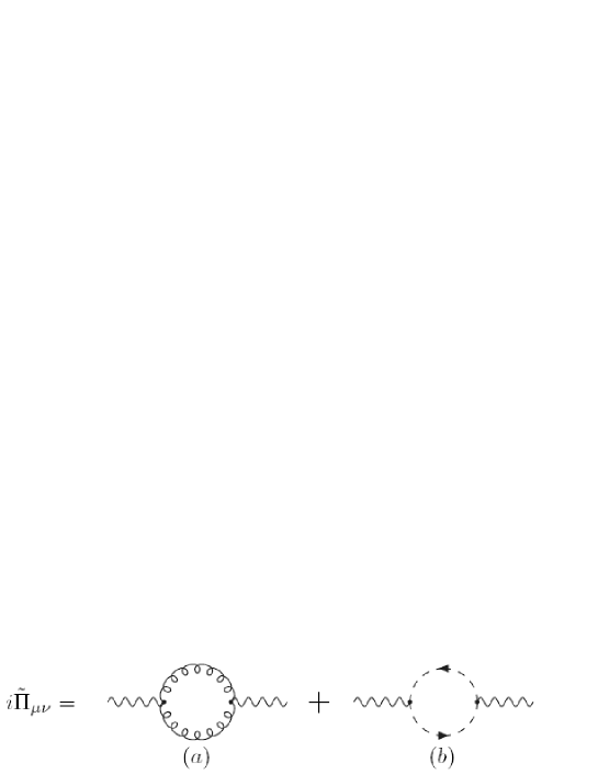
Figure 3: Background gluon self energy.

Now, we calculate the gluon self-energy in the background field method with the background Feynman gauge. Amplitudes of the diagrams 3(a) and 3(b) give the contributions

$$i\widehat{\Pi}^{(a)}_{\mu\nu}(q) = \frac{Ng^{2}}{2}\int\frac{d^{4}k}{(2\pi)^{4}}\frac{1}{k^{2}(k+q)^{2}}\Gamma_{\alpha\mu\beta}^{F}(k,q)\Gamma_{\beta\nu\alpha}^{F}(k+q,-q),$$ (3.19a)

$$i\widehat{\Pi}_{\mu\nu}^{(b)} = -Ng^{2}\int\frac{d^{4}k}{(2\pi)^{4}}\frac{1}{k^{2}(k+q)^{2}}(2k+q)_{\mu}(2k+q)_{\nu},$$ (3.19b)

which correspond respectively to the first and second terms in the expression of the gauge-invariant self-energy $\widehat{\Pi}_{\mu\nu}$ of Eq. (2.29). We proved, by a explicit calculations, that the pinch technique gauge-invariant self-energy of the gluon can be recover easier by the background field method in the Feynman gauge at the one-loop level. We now continue our analysis and show that this equivalence still holds for the 3-gluon and the 4-gluon vertex.

4 Gauge-invariant gluon vertex

4.1 Gauge-independent three-gluon vertex with the intrinsic pinch technique

The calculation of the gauge-invariant three-gluon vertex by the S-matrix pinch technique is much more tedious that for the propagator. The road map of the way the vertex is constructed is given in [6]. But here, we shall just explain the construction of the vertex by the intrinsic pinch technique.

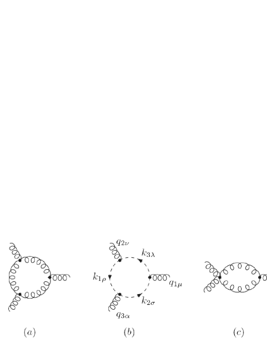
Figure 4: One loop graphs for the conventional 3-gluon vertex.

The relevant graphs for the three-gluon vertex at the one-loop level are depicted in Fig. 4. The contribution of the gluon loop and the symmetrized ghost loop read

$$\Gamma^{\ref{vm:fig:Vertex3g}(a)}_{\mu\nu\alpha} = \frac{iNg^{2}}{2(2\pi)^{4}}\int\frac{d^{4}k}{k^{2}_{1}k^{2}_{2}k^{2}_{3}}\Gamma_{\sigma\mu\lambda}(k_{2},q_{1},-k_{3})\Gamma_{\lambda\nu\rho}(k_{3},q_{2},-k_{1})\Gamma_{\rho\alpha\sigma}(k_{1},q_{3},-k_{2}),$$ (4.1)

$$\Gamma^{\ref{vm:fig:Vertex3g}(b)}_{\mu\nu\alpha} = -\frac{iNg^{2}}{2(2\pi)^{4}}\int\frac{d^{4}k}{k^{2}_{1}k^{2}_{2}k^{2}_{3}}\left(k_{1\nu}k_{2\alpha}k_{3\mu}+k_{1\alpha}k_{2\mu}k_{3\nu}\right),$$ (4.2)

where we omit the group theoretical factor $gf^{abc}$. The momenta and Lorentz indices are defined in Fig. 4(b). All momenta $q_{i}$ are incoming such that $k_{3}=k$, $k_{1}=k+q_{2}$, and $k_{2}=k-q_{1}$. As previously, we rewrite the 3-gluon vertices in $\Gamma^{P}+\Gamma^{F}$ form. We let the $\Gamma^{P}$ generate Ward identities and drop the terms proportional to $q^{2}_{i}$ . The numerator of the gluon loop amplitude can be written as

$$\Gamma^{F}_{1}\Gamma^{F}_{2}\Gamma_{3}^{F}+\Gamma^{P}_{1}\Gamma_{2}\Gamma_{3}+\Gamma_{1}\Gamma^{P}_{2}\Gamma_{3}+\Gamma_{1}\Gamma_{2}\Gamma_{3}^{P}-\Gamma^{P}_{1}\Gamma^{P}_{2}\Gamma_{3}-\Gamma^{P}_{1}\Gamma_{2}\Gamma_{3}^{P}-\Gamma_{1}\Gamma^{P}_{2}\Gamma_{3}^{P}+\Gamma^{P}_{1}\Gamma^{P}_{2}\Gamma_{3}^{P}.$$ (4.3)

Here each vertex labeled $1$ carried the indices $\sigma\mu\lambda$, each vertex labeled $2$ carried the indices $\lambda\nu\rho$, and each vertex labeled $3$ carried the indices $\rho\alpha\sigma$ ; 1,2,3 refer to the exterior momentum labels. For instance, the first term on the RHS of (4.3) really means

$$\Gamma^{F}_{\sigma\mu\lambda}(k_{2},q_{1},-k_{3})\Gamma^{F}_{\lambda\nu\rho}(k_{3},q_{2},-k_{1})\Gamma^{F}_{\rho\alpha\sigma}(k_{1},q_{3},-k_{2}).$$ (4.4)

As with the propagator, the first term on the RHS of (4.3) contains no pinch. Each of the next six terms has pinches (i.e. term in $q^{2}_{i}$) coming from the action of $\Gamma^{P}$ on the full vertex $\Gamma$, via the Ward identities (2.26). Some terms can refer to an internal momentum $k_{i}^{2}$, in which case they give rise to an integral with only two propagators. Let us note that the last term in (4.3), with three $\Gamma^{P}$’s,

$$\begin{split}(\Gamma^{P}_{1}\Gamma^{P}_{2}\Gamma_{3}^{P})_{\mu\nu\alpha}=&k_{3}^{2}(k_{2\mu}g_{\alpha\nu}+k{{}_{1\nu}}g_{\alpha\mu})+k_{2}^{2}(k_{3\mu}g_{\alpha\nu}+k{{}_{1\nu}}g_{\alpha\mu})\\ &+k_{1}^{2}(k_{2\mu}g_{\alpha\nu}+k{{}_{3\nu}}g_{\alpha\mu})+k_{1\nu}k_{2\alpha}k_{3\mu}+k_{1\alpha}k_{2\mu}k_{3\nu},\end{split}$$ (4.5)

yields terms who cancel exactly the ghost contribution since the three first terms vanish by symmetric integration. When we drop the $q_{i}^{2}$ generated by the Ward identity we find the expressions for the others of Eq. (4.3). We have

$$(\Gamma^{P}_{1}\Gamma_{2}\Gamma_{3})_{\mu\nu\alpha} = k_{1}^{2}\left[\Gamma_{\nu\alpha\mu}(k_{1},q_{3},-k_{2})+\Gamma_{\mu\nu\alpha}(k_{3},q_{1},-k_{1})\right]$$ (4.6)

$$-k_{2}^{2}k_{1\nu}g_{\alpha\nu}-k_{3}^{2}k_{1\alpha}g_{\mu\nu}-k_{1\nu}k_{2\alpha}k_{2\mu}+k_{1\alpha}k_{3\mu}k_{3\nu},$$

$$-(\Gamma^{P}_{1}\Gamma_{2}^{P}\Gamma_{3})_{\mu\nu\alpha} = -k_{3}^{2}\Gamma_{\nu\alpha\mu}(k_{1},q_{3},-k_{2})+k_{2}^{2}t_{\alpha\mu}(k_{2})k_{3\nu}+k_{1}^{2}t_{\alpha\nu}(k_{1})k_{3\mu}.$$ (4.7)

Finally, it remains to add the contribution of the graph 4(c) and the two similar ones (by legs permutation). The expression of the gauge-invariant 3-gluon vertex at the one-loop level is then the sum of three terms

$$\widehat{\Gamma}_{\mu\nu\alpha}(q_{1},q_{2},q_{3})=\Gamma_{\mu\alpha\nu}+\frac{iNg^{2}}{2(2\pi)^{4}}\int\frac{d^{4}k}{k^{2}_{1}\ k^{2}_{2}\ k^{2}_{3}}\left(A_{\alpha\mu\nu}+B_{\alpha\mu\nu}\right)-C_{\alpha\mu\nu}.$$ (4.8)

Introducing the notation

$$A(i)=\frac{iNg^{2}}{2(2\pi)^{4}}\int\frac{d^{4}k}{k^{2}(k+q_{i})^{2}},$$ (4.9)

we will see in the following that each of the three terms

$$A_{\alpha\mu\nu} = \Gamma^{F}_{\sigma\mu\lambda}(k_{2},q_{1})\Gamma^{F}_{\lambda\nu\rho}(k_{3},q_{2})\Gamma^{F}_{\rho\alpha\sigma}(k_{1},q_{3}),$$

$$B_{\alpha\mu\nu} = 2(k_{2}+k_{3})_{\mu}(k_{3}+k_{1})_{\nu}(k_{1}+k_{2})_{\alpha},$$

$$C_{\alpha\mu\nu} = 8(q_{1\alpha}g_{\mu\nu}-q_{1\nu}g_{\mu\alpha})A(1)+8(q_{2\mu}g_{\alpha\nu}-q_{2\alpha}g_{\mu\nu})A(2)$$

$$+8(q_{3\nu}g_{\mu\alpha}-q_{3\mu}g_{\nu\alpha})A(3),$$

is equal to a amplitude of a graph in the background field method. We presented here only the ghost and gluon contributions to the one-loop amplitude but the inclusion of fermion and scalar loops are straightforward. Binger and Brodsky found that the forms factor in $d$ dimensions of each contributions satisfy a relation very closely linked to supersymmetry [63].

4.2 Gauge-independent three-gluon vertex with the background field method

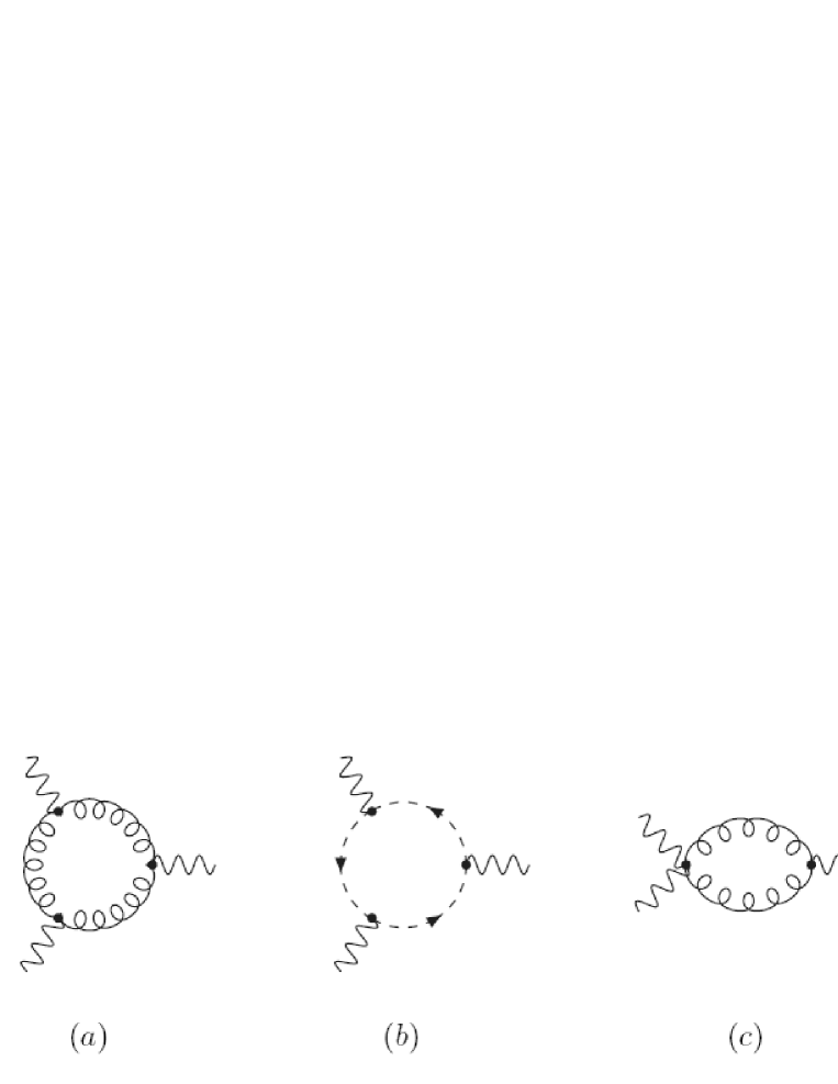
Figure 5: One loop graph for the 3-gluon vertex in the background field method.

We saw in the previous section that the one-loop gluon self-energy derived with the pinch technique can also be obtained, in a easier way, by the background field method in the Feynman gauge. We, now, shall show that the background field method can also be applied to obtain the PT gauge-invariant three gluon vertex at the one-loop level.

The relevant diagrams are shown in Fig. 5, where the conventions for momenta and Lorentz and color indices are displayed in Fig. 4. With the fact that an $AQQ$ vertex in the Feynman gauge, $\widetilde{\Gamma}_{\xi_{Q}=1}$, is equivalent to $\Gamma^{F}$, it is easy to show that the contribution of the diagram 5(a) is

$$\Gamma^{5(a)}_{\mu\nu\alpha}(q_{1},q_{2},q_{3})=\frac{iNg^{2}}{2(2\pi)^{4}}\int\frac{d^{4}k}{k^{2}_{1}k^{2}_{2}k^{2}_{3}}\Gamma^{F}_{\sigma\mu\lambda}(k_{2},q_{1})\Gamma^{F}_{\lambda\nu\rho}(k_{3},q_{2})\Gamma^{F}_{\rho\alpha\sigma}(k_{1},q_{3}).$$ (4.10)

The contribution of the diagram 5(b) (and the similar one with the ghost running the other way) is

$$\Gamma^{5(b)}_{\mu\nu\alpha}(q_{1},q_{2},q_{3})=\frac{iNg^{2}}{(2\pi)^{4}}\int\frac{d^{4}k}{k^{2}_{1}k^{2}_{2}k^{2}_{3}}(k_{2}+k_{3})_{\mu}(k_{3}+k_{1})_{\nu}(k_{1}+k_{2})_{\alpha}.$$ (4.11)

When we calculate the diagram 5(c), again we use the Feynman gauge ($\xi_{Q}=1$) for the four-point vertex with two background fields. Remembering that the diagram 5(c) has a symmetric factor $\frac{1}{2}$ and adding the two other similar diagrams, we find

$$\begin{split}\Gamma^{5(c)}_{\mu\nu\alpha}(q_{1},q_{2},q_{3})=&8(q_{1\alpha}g_{\mu\nu}-q_{1\nu}g_{\mu\alpha})A(1)+8(q_{2\mu}g_{\alpha\nu}-q_{2\alpha}g_{\mu\nu})A(2)\\ &+8(q_{3\nu}g_{\mu\alpha}-q_{3\mu}g_{\nu\alpha})A(3).\end{split}$$ (4.12)

Finally, the contribution of the diagram 5(d) (and two other similar diagrams) turns out to be null because of the group-theoretical identity for the structure constants $f^{abc}$ such as

$$f^{ead}(f^{dbx}f^{xce}+f^{dcx}f^{xbe})=0.$$ (4.13)

Now adding the contributions from the diagrams (a)-(c) in Fig. 5 and omitting the overall group-theoretic factor $gf^{abc}$, we find that the result coincides with the expression of Eq.(4.8) which was obtained by the intrinsic pinch technique. Also we note that each contribution from the diagrams (a)-(c), respectively, corresponds to a particular term in Eq.(4.8).

We close this section with a mention that the constructed $\widehat{\Gamma}_{\mu\nu\alpha}(q_{1},q_{2},q_{3})$ is related to the gauge-invariant propagator $\widehat{\Delta}$ of Eq.(2.32) through a Ward identity

$$q_{1}^{\mu}\widehat{\Gamma}_{\mu\nu\alpha}(q_{1},q_{2},q_{3})=t_{\nu\alpha}(q_{2})\widehat{\Delta}^{-1}(q_{2})-t_{\nu\alpha}(q_{3})\widehat{\Delta}^{-1}(q_{3}),$$ (4.14)

which is indeed a naive extension of the tree-level one. It is very important to note that the Ward identity makes no reference to ghost Green’s functions as the usual covariant-gauge Ward identities do. Finally, we note that the RHS of (4.14) is not a difference of two inverse propagators, because the projection operators $t_{\mu\nu}$ has no inverse.

4.3 Gauge-invariant four-gluon vertex

The construction of the gauge-invariant 4-gluon vertex at the one-loop by the S-matrix pinch technique is described in [64]. This is a tedious work because of the number of the graphs. In addition, new complications arise from the fact that one-particle-reducible and one-particle-irreducible graphs exchange contributions in a nontrivial way. We do not report here the (very) lengthy expression of the vertex but, in his paper, Papavassiliou shows that it obeys the Ward identity

$$\begin{split}q_{1}^{\mu}\widehat{\Gamma}_{\mu\nu\alpha\beta}^{abcd}(q_{1},q_{2},q_{3},q_{4})=&f^{abx}\widehat{\Gamma}^{cdx}_{\nu\alpha\beta}(q_{1}+q_{2},q_{3},q_{4})\\ &+f^{acx}\widehat{\Gamma}^{bdx}_{\nu\alpha\beta}(q_{2},q_{1}+q_{3},q_{4})\\ &+f^{adx}\widehat{\Gamma}^{bcx}_{\nu\alpha\beta}(q_{2},q_{3},q_{1}+q_{4}).\end{split}$$ (4.15)

which is a extension of the tree-level one. In this equation, in the same way we defined the 3-gluon vertex $g\widehat{\Gamma}^{cdx}_{\nu\alpha\beta}$, we defined the 4-gluon vertex by $-ig^{2}\widehat{\Gamma}_{\mu\nu\alpha\beta}^{abcd}$.

The construction of the gauge-invariant 4-gluon vertex was also done in [65] in the context of the background field method. The relevant graph and their amplitude can be found in this reference. It is also proved that the 4-gluon vertex satisfies the same Ward identity that the pinch technique one. Hence we are lead to the conclusion that (at least) the longitudinal parts of the two vertex $\tilde{\Gamma}_{\mu\nu\alpha\beta}^{abcd}$ (with 4 background gluons) and $\widehat{\Gamma}_{\mu\nu\alpha\beta}^{abcd}$ are equal.

5 First principles and mathematical tools

Quantum field theory is based on fundamental principles, such as the conservation of probability, causality, analyticity or gauge invariance. Using these assumptions, we shall derive constraints on the Green’s functions of the theory, namely the dispersion relations, the optical theorem and the Ward identities.

5.1 Analyticity and renormalization

Analyticity is one of the most important properties that governs physical transition amplitudes. Correlation functions are considered to be analytic in their kinematic variables, which is expressed by means of the so-called Dispersion Relations (DRs) [53, 54, 55]. They were first derived in optics as a consequence of analyticity and causality. In this section, we briefly review some important facts about DRs and renormalization and discuss the subtleties encountered in non-Abelian gauge theories.

If a complex function $f(z)$ is analytic in the interior of and upon a closed curve, $C_{\uparrow}$ shown in Fig. 6, and $x+i\varepsilon$ (with $x,\varepsilon\in$ R and $\varepsilon>0$) is a point within the closed curve $C_{\uparrow}$, we then have the Cauchy’s integral form,

$$f(x+i\varepsilon)\ =\ \frac{1}{2\pi i}\oint_{C_{\uparrow}}dz\,\frac{f(z)}{z-x-i\varepsilon}\ ,$$ (5.1)

where $\oint$ denotes that the path $C_{\uparrow}$ is singly wound. Using Schwartz’s reflection principle, one also obtains

$$f(x-i\varepsilon)\ =\ -\,\frac{1}{2\pi i}\oint_{C_{\downarrow}}dz\,\frac{f(z)}{z-x+i\varepsilon}\ .$$ (5.2)

Note that $C_{\uparrow}^{*}=C_{\downarrow}$. Sometimes, an analytic function is called holomorphic; both terms are equivalent for complex functions.

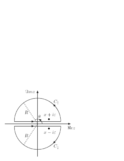
Figure 6: Contours of complex integration.

Of significant importance in the discussion of physical processes is a DR, which relates the imaginary part of an analytic function $f(x)$ to its real part, and vice versa. We assume for the moment that the analytic function $f(z)$ has the asymptotic behaviour $|f(z)|\leq C/R^{k}$, for large radii $R$, where $C$ is a real nonnegative constant and $k>0$; this assumption will be relaxed later on, giving rise to more involved DR. Taking now the limit $\varepsilon\to 0$, it is easy to evaluate $\Re ef(x)$ through

$$2\Re ef(x)\ =\ `\lim_{\varepsilon\to 0}\mbox{'}\Big{[}f(x+i\varepsilon)+f^{*}(x-i\varepsilon)\Big{]}\ =\ `\lim_{\varepsilon\to 0}\mbox{'}\,\frac{1}{\pi}\int\limits_{-\infty}^{+\infty}dx^{\prime}\,\Im m\left(\frac{f(x^{\prime})}{x^{\prime}-x-i\varepsilon}\right)\,+\,\Gamma_{\infty}.$$ (5.3)

Here, $`\lim_{\varepsilon\to 0}\mbox{'}$ means that the limit should be taken after the integration has been performed, and

$$\Gamma_{\infty}\ =\ \frac{1}{\pi}\lim_{R\to\infty}\,\Re e\,\int_{0}^{\pi}d\theta\,f(Re^{i\theta})\,.$$ (5.4)

Because of the assumed asymptotic behaviour of $f(z)$ at infinity, the integral over the upper infinite semicircle in Fig. 1, $\Gamma_{\infty}$, can be easily shown to vanish. Employing the well-known identity for distributions (the symbol P in front of the integral stands for principle value integration),

$$`\lim_{\varepsilon\to 0}\mbox{'}\,\frac{1}{x^{\prime}-x-i\varepsilon}\ =\ \mbox{P}\frac{1}{x^{\prime}-x}\ +\ i\pi\delta(x^{\prime}-x),$$

we arrive at the unsubtracted dispersion relation,

$$\Re ef(x)\ =\ \frac{1}{\pi}\,\mbox{P}\,\int\limits^{+\infty}_{-\infty}dx^{\prime}\,\frac{\Im mf(x^{\prime})}{x^{\prime}-x}\ .$$ (5.5)

Following a similar line of arguments, one can express the imaginary part of $f(x)$ as an integral over $\Re ef(x)$.

In the previous derivation, the assumption that $|f(z)|$ approaches zero sufficiently fast at infinity has been crucial, since it guarantees that $\Gamma_{\infty}\to 0$. However, if we were to relax this assumption, additional subtractions need to be included in order to arrive at a finite expression. For instance, for $|f(z)|\leq CR^{k}$ with $k<1$, it is sufficient to carry out a single subtraction at a point $x=a$. In this way, one has

$$\Re ef(x)\ =\ \Re ef(a)\ +\ \frac{(x-a)}{\pi}\,\mbox{P}\,\int\limits_{-\infty}^{+\infty}dx^{\prime}\,\frac{\Im mf(x^{\prime})}{(x^{\prime}-a)(x^{\prime}-x)}\ .$$ (5.6)

From Eq. (5.6), $\Re ef(x)$ can be obtained from $\Im mf(x)$, up to a unknown, real constant $\Re ef(a)$. Usually, the point $a$ is chosen in a way such that $\Re ef(a)$ takes a specific value on account of some physical requirement. For example, if $\Im mf(q^{2})$ is the imaginary part of the magnetic form factor of an electron with photon virtuality $q^{2}$, one can prescribe that the physical condition $\Re ef(0)=0$ should hold true in the Thomson limit.

We next focus on the study of some crucial analytic properties of off-shell transition amplitudes within the context of renormalizable field theories. In such theories, one is allowed to have at most two subtractions for a two-point correlation function. If $\Pi(s=q^{2})$ is the self-energy function of a scalar particle with mass $m$ and off-shell momentum $q$ —the fermionic or vector case is analogous— then the real (or dispersive) part of this amplitude can be fully determined by its imaginary (or absorptive) part via the expression

$$\Re e\Pi(s)\ =\ \Re e\Pi(m^{2})\,+\,(s-m^{2})\Re e\Pi^{\prime}(m^{2})\,+\,\frac{(s-m^{2})^{2}}{\pi}\mbox{P}\,\int\limits_{0}^{+\infty}ds^{\prime}\,\frac{\Im m\Pi(s^{\prime})}{(s^{\prime}-m^{2})^{2}(s^{\prime}-s)}\ .\quad$$ (5.7)

From Eq. (5.7), one can readily see that the two subtractions, $\Re e\Pi(m^{2})$ and the derivative $\Re e\Pi^{\prime}(m^{2})$, respectively correspond to the mass and wave-function renormalization constants in the on-mass shell scheme. At higher orders, internal renormalizations of $\Im m\Pi(s)$, due to counterterms coming from lower orders, should also be taken into account. Then, Eq. (5.7) is still valid, i.e., it holds to order $n$ provided $\Im m\Pi(s)$ is renormalized to order $n-1$. In general, the function $\Im m\Pi(s)$ has its support in the non-negative real axis, i.e., for $s\geq 0$. This can be attributed to the semi-boundness of the spectrum of the Hamiltonian, Spec$H\geq 0$ [56]. Note that for spectrally represented two-point correlation functions, we have the additional condition $\Im m\Pi(m^{2})\geq 0~{}$[57, 58].

As has been mentioned above, in renormalizable field theories it is required that $\Pi(s)$ should be finite after two subtractions have been performed. This implies that

$$|\Pi(s)|\ \leq\ Cs^{k}\,,\qquad\mbox{with}\quad k<2,$$ (5.8)

as $s\to\infty$. Obviously, the same inequality holds true for the real as well as the imaginary part of $\Pi(s)$. In pure non-abelian Yang-Mills theories, such as quark-less QCD, the transverse part, $\Pi_{T}(s)$, of the gluon vacuum polarization behaves asymptotically as, see Eq. (2.31),

$$\Pi_{T}(s)\ \to\ C\,s\Big{(}\ln\frac{s}{\mu^{2}}\Big{)}^{n}\ .$$

This result is consistent with Eq. (5.8), for any $n<\infty$. Furthermore, we mention in passing that the Froissart–Martin bound [3],

$$|\Pi(s)|\ \leq\ C\,s^{3}\Big{(}\ln\frac{s}{s_{0}}\Big{)}^{2},$$ (5.9)

at $s\to\infty$, which may be derived from axiomatic methods of field theory, is weaker than Eq. (5.8). In fact, the Froissart-Martin bound [3] refers to the asymptotic behaviour of a total cross section, $\sigma(s)$, in the limit $s\to\infty$. This is expressed as $\sigma(s)\,\leq\,C[\ln(s/s_{0})]^{2}$. Furthermore, the optical theorem gives the relation $s\,\sigma(s)=\Im mT(s)$, where $T(s)$ is the forward-scattering amplitude. If one assumes the absence of accidental cancellations between the two-point function, $\Pi(s)$, and higher $n$-point functions within the expression $\Im mT(s)$, one can derive that

$$|\Im m\Pi(s)|\,\leq\,Cs^{2}\Im mT(s)\,\leq\,Cs^{3}[\ln(s/s_{0})]^{2}.$$

Because of analyticity, the $s$-dependence of $\Im m\Pi(s)$ will affect the high-$s$ behaviour of $|\Pi(s)|$. Even if we assume that the $s$-dependence thus induced on $|\Pi(s)|$ is the most modest possible, i.e., $|\Pi(s)|\sim\Im m\Pi(s)$ as $s\rightarrow\infty$, still the tightest upper bound one could obtain from these considerations is that of Eq. (5.9). The analytic expression of gluon vacuum polarization satisfies Eq. (5.9). As a counter-example to this situation, we may consider the Higgs self-energy in the unitary gauge; the absorptive part of the Higgs self-energy has an $s^{2}$ dependence at high energies, and its resummation [59] is therefore not justified.

In the context of gauge field theories, one should anticipate a similar analytic structure for two-point correlation functions. However, an extra complication appears in such theories when off-shell transition amplitudes are considered. In a theory with spontaneous symmetry breaking, such as the Standard Model for example, this complication originates from the fact that, in addition to the physical particles of the spectrum of the Hamiltonian, unphysical gauge dependent degrees of freedom, such as would-be Goldstone bosons and ghost fields make their appearance. Although on-shell transition amplitudes contain only the physical degrees of freedom of the particles involved on account of unitarity, their continuation to the off-shell region is ambiguous, because of the presence of unphysical Landau poles, introduced by the aforementioned unphysical particles. A reasonable prescription for accomplishing such an off-shell continuation, which is very close in spirit to the previous example of the scalar theory, would be to continue analytically an off-shell amplitude by taking only physical Landau singularities into account.

Consider for example the off-shell propagator of a gauge particle in the conventional $R_{\xi}$ gauges or BFGs, which runs inside a quantum loop,

$$\Delta_{0\mu\nu}^{(\xi_{Q})}(q)\ =\ t_{\mu\nu}(q)\,\frac{-i}{q^{2}-M^{2}}\,-\,\ell_{\mu\nu}(q)\,\frac{i\xi_{Q}}{q^{2}-\xi_{Q}M^{2}}\ ,\text{ with}\quad\ell_{\mu\nu}(q)\ =\ \frac{q_{\mu}q_{\nu}}{q^{2}}\ .$$ (5.10)

One can write two separate DRs for the transverse self-energy, $\Pi_{T}$, of a massive gauge boson, which crucially depend on the pole structure of Eq. (5.10), namely

$$\Re e\bar{\Pi}_{T}(s) = \Re e\bar{\Pi}_{T}(M^{2})+(s-M^{2})\Re e\bar{\Pi}^{\prime}_{T}(M^{2})+\frac{(s-M^{2})^{2}}{\pi}$$ (5.11)

$$\times\mbox{P}\,\int\limits_{\{M^{2}_{phys}\}}^{+\infty}ds^{\prime}\,\frac{\Im m\bar{\Pi}_{T}(s^{\prime})}{(s^{\prime}-M^{2})^{2}(s^{\prime}-s)}\,,$$

$$\Re e\bar{\Pi}^{(\xi_{Q})}_{T}(s) = (s-M^{2})\Re e\bar{\Pi}^{\prime(\xi_{Q})}_{T}(M^{2})+\frac{(s-M^{2})^{2}}{\pi}\mbox{P}\,\int\limits_{\{M^{2}_{unphys}\}}^{+\infty}ds^{\prime}\,\frac{\Im m\bar{\Pi}_{T}^{(\xi_{Q})}(s^{\prime})}{(s^{\prime}-M^{2})^{2}(s^{\prime}-s)}\,.$$

In the first DR given in Eq. (5.11), the real part of $\Pi_{T}$, $\Re e\bar{\Pi}_{T}$, is determined from branch cuts induced by physical poles, where the masses of the real on-shell particles in the loop are collectively denoted by $\{M^{2}_{phys}\}$. In what follows we refer to such a DR as physical DR. Note that $\Re e\bar{\Pi}_{T}$ depends only implicitly on the gauge choice. In fact, $\Re e\bar{\Pi}_{T}$ can be viewed as the truncated part of the self-energy that will survive if $\Re e{\Pi}_{T}$ is embedded in a $S$-matrix element. In Eq. (5.1), the dispersive part of the two-point function depends explicitly on $\xi_{Q}$-dependent unphysical thresholds, collectively denoted by $\{M^{2}_{unphys}\}$, which are induced by the longitudinal parts of the gauge propagators contained in $\Im m\bar{\Pi}_{T}^{(\xi_{Q})}$. Evidently, one has the decomposition

$$\Im m\Pi_{T}(s)\ =\ \Im m\bar{\Pi}_{T}(s)+\Im m\bar{\Pi}_{T}^{(\xi_{Q})}(s)\,,\quad\Re e\Pi_{T}(s)\ =\ \Re e\bar{\Pi}_{T}(s)+\Re e\bar{\Pi}_{T}^{(\xi_{Q})}(s)\,.$$ (5.13)

From Eq. (5.10), one can now isolate that part of the propagator that should be used in a physical DR. For $\xi_{Q}\not=1$, one has

$$\Delta_{0\mu\nu}^{(\xi_{Q})}\ \to\ U_{\mu\nu}(q)\ \equiv\ \Delta_{0\mu\nu}^{(\infty)}(q)\,.$$ (5.14)

It is therefore obvious that the ‘physical’ sector of an off-shell transition amplitude in BFG (for $\xi_{Q}\not=1$) —or equivalently, the part of the off-shell matrix element that satisfies a physical DR— is effectively obtained by considering all the internal propagators in the unitary gauge ($\xi_{Q}\to\infty$), but leaving the Feynman rules for the vertices in the general $\xi_{Q}$ gauge.

In view of a physical DR, the gauge $\xi_{Q}=1$ is very specific, since the physical and unphysical poles coincide in such a case, making them indistinguishable. At one-loop order, the results of this gauge are found to collapse to those obtained via the PT [48]. Finally we remark in passing that, if $\bar{\Pi}_{T}$ in $\xi_{Q}\not=1$ is used for a definition of a ‘physical’ self-energy, one encounters problems with the high-energy unitarity behaviour, even though the full $\Pi(\xi_{Q})$ is asymptotically well-behaved. In the case of the one-loop $Z$ self-energy for example, for $\xi_{Q}\not=1$ [48], $\bar{\Pi}_{T}$ contains terms proportional to $q^{4}$; all such terms eventually cancel in the entire $\Pi(\xi_{Q})$ against the part that contains the unphysical poles. Incidentally, it is interesting to notice that the recovery of the correct asymptotic behaviour is the more delayed, i.e., it happens for larger values of $q^{2}$, the larger the value of $\xi_{Q}$. However, if one was to resum only the $\bar{\Pi}_{T}$ part, the terms proportional to $q^{4}$ would survive, leading to bad high energy behaviour. If, on the other hand, one had resummed the full $\Pi(\xi_{Q})$, then one would have introduced unphysical poles, as explained above.

5.2 Unitarity and gauge invariance

In this section, we will briefly discuss the basic field-theoretical consequences resulting from the unitarity of the $S$-matrix theory, and establish its connection with gauge invariance. In addition to the requirement of explicit gauge invariance, the necessary conditions derived from unitarity will constitute our guiding principle to analytically continue $n$-point correlation functions in the off-shell region. Furthermore, we arrive at the important conclusion that the resummed self-energies, in addition to being GFP independent, must also be “unitary”, in the sense that they do not spoil unitarity when embedded in an $S$-matrix element.

The $T$-matrix element of a reaction $i\to f$ is defined via the relation

$$\langle f|S|i\rangle\ =\ \delta_{fi}\ +\ i(2\pi)^{4}\delta^{(4)}(P_{f}-P_{i})\langle f|T|i\rangle,$$ (5.15)

where $P_{i}$ ($P_{f}$) is the sum of all initial (final) momenta of the $|i\rangle$ ($|f\rangle$) state. Furthermore, imposing the unitarity relation $S^{\dagger}S=1$, consequence of the conservation of the probability, leads to the optical theorem:

$$\langle f|T|i\rangle-\langle i|T|f\rangle^{*}\ =\ i\sum_{i^{\prime}}(2\pi)^{4}\delta^{(4)}(P_{i^{\prime}}-P_{i})\langle i^{\prime}|T|f\rangle^{*}\langle i^{\prime}|T|i\rangle.$$ (5.16)

In Eq. (5.16), the sum $\sum_{i^{\prime}}$ should be understood to be over the entire phase space and spins of all possible on-shell intermediate particles $i^{\prime}$. A corollary of this theorem is obtained if $i=f$. In this particular case, we have

$$2\Im m\langle i|T|i\rangle\ =\sum_{f}(2\pi)^{4}\delta^{(4)}(P_{f}-P_{i})|\langle f|T|i\rangle|^{2}.$$ (5.17)

In the conventional $S$-matrix theory with stable particles, Eqs (5.16) and (5.17) hold also perturbatively. To be precise, if one expands the transition $T=T^{(1)}+T^{(2)}+\cdots+T^{(n)}+\cdots$, to a given order $n$, one has

$$T^{(n)}_{fi}-T^{(n)*}_{if}\ =\ i\sum_{i^{\prime}}(2\pi)^{4}\delta^{(4)}(P_{i^{\prime}}-P_{i})\sum\limits_{k=1}^{n-1}T^{(k)*}_{i^{\prime}f}T^{(n-k)}_{i^{\prime}i}.$$ (5.18)

There are two important conclusions that can be drawn from Eq. (5.18). First, the anti-hermitian part of the LHS of Eq. (5.18) contains, in general, would-be Goldstone bosons or ghost fields [60]. Such contributions manifest themselves as Landau singularities at unphysical points, e.g., $q^{2}=\xi_{Q}M_{W}^{2}$ for a $W$ propagator in a general BFG. However, unitarity requires that these unphysical contributions should vanish, as can be read off from the RHS of Eq. (5.18). Second, the RHS explicitly shows the connection between gauge invariance and unitarity at the quantum loop level. To lowest order for example, the RHS consists of the product of GFP independent on-shell tree amplitudes, thus enforcing the gauge-invariance of the imaginary part of the one-loop amplitude on the LHS.

The above powerful constraints imposed by unitarity will be in effect as long as one computes full amplitudes to a finite order in perturbation theory. However, for resummation purposes, a certain sub-amplitude, i.e., a part of the full amplitude, must be singled out and subsequently undergo a Dyson summation, while the rest of the $S$-matrix is computed to a finite order $n$. Therefore, if the resummed amplitude contains gauge artifacts and/or unphysical thresholds, the cancellations imposed by Eq. (5.18) will only operate up to order $n$, introducing unphysical contributions of order $n+1$ or higher. To avoid the contamination of the physical amplitudes by such unphysical artifacts, we impose the following two requirements on the effective Green’s functions, when one attempts to continue them analytically in the off-shell region for the purpose of resummation:

• The off-shell $n$-point correlation functions ought to be derivable from or embeddable into $S$-matrix elements.

• The off-shell Green’s functions should not display unphysical thresholds induced by unphysical Landau singularities, as has been described above.

Even though property (i) is automatic for Green’s functions generated by the functional differentiation of the conventional path-integral functional, in general the off-shell amplitudes so obtained fail to satisfy property (ii). In the PT framework instead, both conditions are satisfied: Effective Green’s functions are directly derived from the $S$-matrix amplitudes (so condition (i) is satisfied by construction) and contain only physical thresholds, so that unitarity is not explicitly violated [10].

In our discussion of unitarity at one-loop, we will make extensive use of the following two-body Lorentz-invariant phase-space (LIPS) integrals: The scalar integral

$$\int dX_{LIPS} = \frac{1}{(2\pi)^{2}}\,\int d^{4}k_{1}\int d^{4}k_{2}\,\delta_{+}(k^{2}_{1}-m^{2}_{1})\delta_{+}(k^{2}_{2}-m^{2}_{2})\delta^{(4)}(q-k_{1}-k_{2})$$ (5.19)

$$= \theta(q^{0})\theta[q^{2}-{(m_{1}+m_{2})}^{2}]\,\frac{1}{8\pi\,q^{2}}\,\lambda^{1/2}(q^{2},m_{1}^{2},m_{2}^{2})\,,$$

where $\lambda(x,y,z)=(x-y-z)^{2}-4yz$ and $\delta_{+}(k^{2}-m^{2})\equiv\theta(k^{0})\delta(k^{2}-m^{2})$, and the tensor integral:

$$\int dX_{LIPS}{(k_{1}-k_{2})}_{\mu}{(k_{1}-k_{2})}_{\nu} = \Big{\{}\frac{\lambda(q^{2},m_{1}^{2},m_{2}^{2})}{3q^{2}}\,t_{\mu\nu}(q)+\,\Big{[}\frac{\lambda(q^{2},m_{1}^{2},m_{2}^{2})}{q^{2}}-q^{2}$$ (5.20)

$$+2(m^{2}_{1}+m^{2}_{2})\Big{]}\,\ell_{\mu\nu}(q)\,\Big{\}}\times\int dX_{LIPS}\,.$$

6 The absorptive pinch technique construction

6.1 Forward scattering in QCD

In this section, we show that a self-consistent picture may be obtained by resorting to such fundamental properties of the $S$-matrix as unitarity and analyticity, using as additional input only elementary Ward identities (EWIs) for tree-level, on-shell processes, and tree-level vertices and propagators. It is important to emphasize that the gauge-fixing parameter (GFP) independence of the results emerges automatically from the previous considerations.

We begin from the right-hand-side (RHS) of the optical relation given in Eq. (5.17). The RHS involves on-shell physical processes, which satisfy the EWIs. It turns out that the full exploitation of those EWIs leads unambiguously to a decomposition of the tree-level amplitude into propagator-, vertex- and box-like structures. The propagator-like structure corresponds to the imaginary part of the effective propagator under construction. By imposing the additional requirement that the effective propagator be an analytic function of $q^{2}$ one arrives at a dispersion relation (DR), which, up to renormalization-scheme choices, leads to a unique result for the real part.

Consider the forward scattering process $q{\bar{q}}\rightarrow q{\bar{q}}$. From the optical theorem, we then have

$$2\Im m\langle q\bar{q}|T|q\bar{q}\rangle\ =\left(\frac{1}{2}\right)\,\int dX_{LIPS}\,\langle q\bar{q}|T|gg\rangle\langle gg|T|q\bar{q}\rangle^{*}\,.$$ (6.1)

In Eq. (6.1), the statistical factor 1/2 in parentheses arises from the fact that the final on-shell gluons should be considered as identical particles in the total rate. We consider only physical gluon as intermediate states. The inclusion of quarks will lead to the contribution of the quark loop in the self-energy. We now set ${\cal M}=\langle q\bar{q}|T|q\bar{q}\rangle$ and ${\cal T}=\langle q\bar{q}|T|gg\rangle$, and focus on the RHS of Eq. (6.1). Diagrammatically, the amplitude ${\cal T}$ consists of two distinct parts: $t$ and $u$-channel graphs that contain an internal quark propagator, ${{\cal T}_{t}}^{ab}_{\mu\nu}$, as shown in Figs. 7(a) and 7(b), and an $s$-channel amplitude, ${{\cal T}_{s}}^{ab}_{\mu\nu}$, which is given in Fig. 7(c). The subscript “$s$” and “$t$” refers to the corresponding Mandelstam variables, i.e. $s=q^{2}=(p_{1}+p_{2})^{2}=(k_{1}+k_{2})^{2}$, and $t=(p_{1}-k_{1})^{2}=(p_{2}-k_{2})^{2}$. Defining the quark current

$$V_{\rho}^{c}\ =\ g\bar{v}(p_{2})\,\frac{\lambda^{c}}{2}\gamma_{\rho}\,u(p_{1})\,,$$ (6.2)

we have that

$${\cal T}^{ab}_{\mu\nu}={{\cal T}_{s}}^{ab}_{\mu\nu}(\xi)+{{\cal T}_{t}}^{ab}_{\mu\nu}\,,$$ (6.3)

with

$${{\cal T}_{s}}^{ab}_{\mu\nu}(\xi) = -gf^{abc}\,\Delta^{(\xi),\rho\lambda}_{0}(q)\Gamma_{\lambda\mu\nu}(q,-k_{1},-k_{2})\,V_{\rho}^{c}\,,$$ (6.4)

$${{\cal T}_{t}}^{ab}_{\mu\nu} = -ig^{2}\bar{v}(p_{2})\Big{(}\,\frac{\lambda^{b}}{2}\gamma^{\nu}\,\frac{1}{\not\!p_{1}-\not\!k_{1}-m}\,\frac{\lambda^{a}}{2}\gamma^{\mu}\ +\ \frac{\lambda^{a}}{2}\gamma^{\mu}\,\frac{1}{\not\!p_{1}-\not\!k_{2}-m}\,\gamma^{\nu}\frac{\lambda^{b}}{2}\,\Big{)}u(p_{1})\,,\qquad$$ (6.5)

where

$$\Gamma_{\lambda\mu\nu}(q,-k_{1},-k_{2})\ =\ (k_{1}-k_{2})_{\lambda}g_{\mu\nu}\,+\,(q+k_{2})_{\mu}g_{\lambda\nu}\,-\,(q+k_{1})_{\nu}g_{\lambda\nu}\,.$$ (6.6)

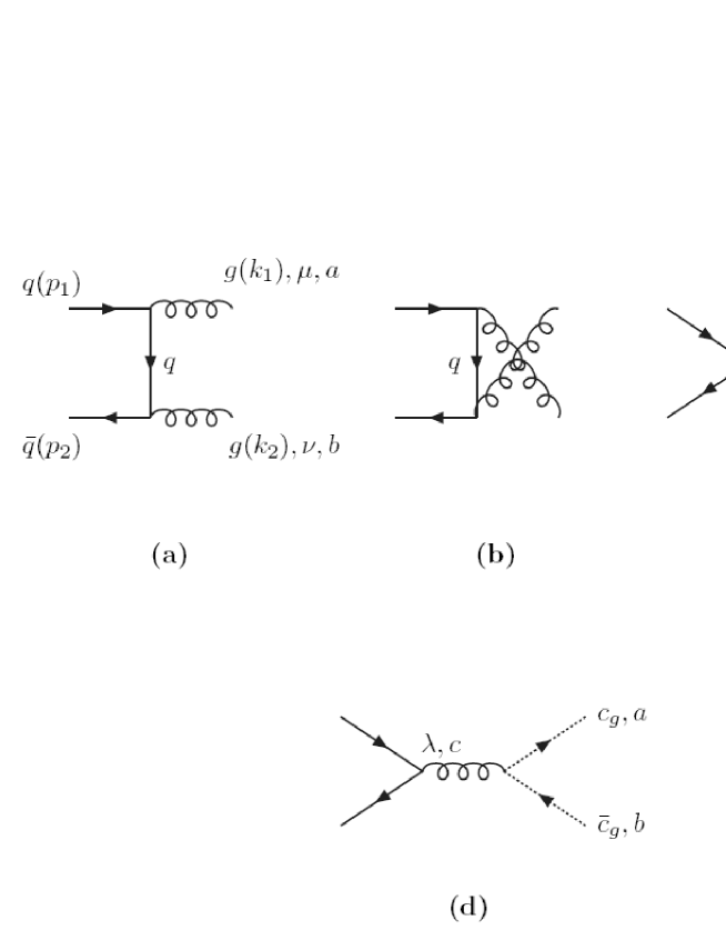
Figure 7: Diagrams (a)–(c) contribute to ${\cal T}^{ab}_{\mu\nu}$, and diagram (d) to ${\cal S}^{ab}$.

Notice that ${\cal T}_{s}$ depends explicitly on the GFP $\xi$, through the tree-level gluon propagator $\Delta^{(\xi)}_{0\mu\nu}(q)$, whereas ${\cal T}_{t}$ does not. The explicit expression of $\Delta^{(\xi)}_{0\mu\nu}(q)$ depends on the specific gauge fixing procedure chosen. In addition, we define the quantities ${\cal S}^{ab}$ and ${\cal R}^{ab}_{\mu}$ as follows:

$${\cal S}^{ab} = gf^{abc}\,\frac{k^{\sigma}_{1}}{q^{2}}\,V_{\sigma}^{c}=-gf^{abc}\,\frac{k^{\sigma}_{2}}{q^{2}}\,V_{\sigma}^{c}$$ (6.7)

and

$${\cal R}_{\mu}^{ab}\ =\ gf^{abc}\,V_{\mu}^{c}\,.$$ (6.8)

Clearly,

$$k_{1}^{\sigma}{\cal R}_{\sigma}^{ab}\ =\ -k_{2}^{\sigma}{\cal R}_{\sigma}^{ab}\ =\ q^{2}{\cal S}^{ab}.$$ (6.9)

We then have

$$\Im m{\cal M} = \frac{1}{4}\,{\cal T}^{ab}_{\mu\nu}\,P^{\mu\sigma}(k_{1},\eta_{1})\,P^{\nu\lambda}(k_{2},\eta_{2})\,{\cal T}^{ab*}_{\sigma\lambda}$$ (6.10)

$$= \frac{1}{4}\Big{[}{{\cal T}_{s}}^{ab}_{\mu\nu}(\xi)+{{\cal T}_{t}}^{ab}_{\mu\nu}\Big{]}\,P^{\mu\sigma}(k_{1},\eta_{1})\,P^{\nu\lambda}(k_{2},\eta_{2})\,\Big{[}{{\cal T}_{s}}^{ab*}_{\sigma\lambda}(\xi)+{{\cal T}_{t}}^{ab*}_{\sigma\lambda}\Big{]},$$

where the polarization tensor $P^{\mu\nu}(k,\eta)$ is given by

$$\sum_{\text{Phys.}}\epsilon_{\mu}^{a}(k)\epsilon_{\nu}^{a}(k)=P_{\mu\nu}(k,\eta)\ =\ -g_{\mu\nu}+\frac{\eta_{\mu}k_{\nu}+\eta_{\nu}k_{\mu}}{\eta k}+\eta^{2}\frac{k_{\mu}k_{\nu}}{{(\eta k)}^{2}}\,.$$ (6.11)

Moreover, we have that on-shell, i.e., for $k^{2}=0$, $k^{\mu}P_{\mu\nu}=0$. By virtue of this last property, we see immediately that if we write the three-gluon vertex of Eq. (6.6) in the form

$$\Gamma_{\lambda\mu\nu}(q,-k_{1},-k_{2}) = [(k_{1}-k_{2})_{\lambda}g_{\mu\nu}+2q_{\mu}g_{\lambda\nu}-2q_{\nu}g_{\lambda\mu}]\ +\ (-k_{1\mu}g_{\lambda\nu}+k_{2\nu}g_{\lambda\mu})$$ (6.12)

$$= \Gamma^{F}_{\lambda\mu\nu}(q,-k_{1},-k_{2})\ +\ \Gamma^{P}_{\lambda\mu\nu}(q,-k_{1},-k_{2})\,,$$

the term $\Gamma^{P}_{\rho\mu\nu}$ dies after hitting the polarization vectors $P_{\mu\sigma}(k_{1},\eta_{1})$ and $P_{\nu\lambda}(k_{2},\eta_{2})$. Therefore, if we denote by ${\cal T}_{s}^{F}(\xi)$ the part of ${\cal T}_{s}$ which survives, Eq. (6.10) becomes

$$\Im m{\cal M}\ =\ \frac{1}{4}\,\big{[}{\cal T}_{s}^{F}(\xi)+{\cal T}_{t}\big{]}^{ab}_{\mu\nu}\,P^{\mu\sigma}(k_{1},\eta_{1})\,P^{\nu\lambda}(k_{2},\eta_{2})\,\big{[}{\cal T}_{s}^{F}(\xi)+{\cal T}_{t}\big{]}^{ab*}_{\sigma\lambda}\,.$$ (6.13)

The next step is to verify that any dependence on the GFP inside the propagator $\Delta^{(\xi)}_{0\mu\nu}(q)$ of the off-shell gluon will disappear. This is indeed so, because the longitudinal parts of $\Delta_{0\mu\nu}$ either vanish because the external quark current is conserved, or because they trigger the following EWI:

$$q^{\mu}\Gamma^{F}_{\mu\alpha\beta}(q,-k_{1},-k_{2})\ =\ (k_{1}^{2}\ -\ k_{2}^{2})g_{\alpha\beta}\,,$$ (6.14)

which vanishes on shell. This last EWI is crucial, because in general, current conservation alone is not sufficient to guarantee the GFP independence of the final answer. In the covariant gauges for example, the gauge fixing term is proportional to $q^{\mu}q^{\nu}$; current conservation kills such a term. But if we had chosen an axial gauge instead, i.e.

$$\Delta^{(\tilde{\eta})}_{0\mu\nu}(q)\ =\ \frac{iP_{\mu\nu}(q,\tilde{\eta})}{q^{2}}\,,$$ (6.15)

where $\tilde{\eta}\neq\eta$ in general, then only the term ${\tilde{\eta}_{\nu}}q_{\mu}$ vanishes because of current conservation, whereas the term ${\tilde{\eta}_{\mu}}q_{\nu}$ can only disappear if Eq. (6.14) holds. So, Eq. (6.13) becomes

$$\Im m{\cal M}\ =\ \frac{1}{4}({\cal T}_{s}^{F}+{\cal T}_{t})^{ab}_{\mu\nu}\,P^{\mu\sigma}(k_{1},\eta_{1})\,P^{\nu\lambda}(k_{2},\eta_{2})\,({\cal T}_{s}^{F}+{\cal T}_{t})^{ab*}_{\sigma\lambda}\,,$$ (6.16)

where the GFP-independent quantity ${\cal T}_{s}^{F}$ is given by

$${{\cal T}_{s}}^{F,ab}_{\mu\nu}\ =\ -gf^{abc}\,\frac{g^{\rho\lambda}}{q^{2}}\,\,\Gamma^{F}_{\lambda\mu\nu}(q,-k_{1},-k_{2})\,V_{\rho}^{c}\,.$$ (6.17)

Next, we want to show that the dependence on $\eta_{\mu}$ and $\eta^{2}$ stemming from the polarization vectors disappears. Using the on shell conditions $k_{1}^{2}=k_{2}^{2}=0$, we can easily verify the following EWIs:

$$k_{1}^{\mu}{{\cal T}_{s}}^{F,ab}_{\mu\nu} = 2k_{2\nu}{\cal S}^{ab}\,-\,{\cal R}_{\nu}^{ab}\,,$$ (6.18)

$$k_{2}^{\nu}{{\cal T}_{s}}^{F,ab}_{\mu\nu} = 2k_{1\mu}{\cal S}^{ab}\,+\,{\cal R}_{\mu}^{ab}\,,$$ (6.19)

$$k_{1}^{\mu}{{\cal T}_{t}}^{ab}_{\mu\nu} = {\cal R}_{\nu}^{ab}\,,$$ (6.20)

$$k_{2}^{\nu}{{\cal T}_{t}}^{ab}_{\mu\nu} = -{\cal R}_{\mu}^{ab}\,,$$ (6.21)

from which we have that

$$k_{1}^{\mu}k_{2}^{\nu}{{\cal T}_{s}}^{F,ab}_{\mu\nu} = q^{2}{\cal S}^{ab}\,,$$ (6.22)

$$k_{1}^{\mu}k_{2}^{\nu}{{\cal T}_{t}}^{ab}_{\mu\nu} = -q^{2}{\cal S}^{ab}\,.$$ (6.23)

Using the above EWIs, it is now easy to check that indeed, all dependence on both $\eta_{\mu}$ and $\eta^{2}$ cancels in Eq. (6.16), as it should, and we are finally left with (omitting the fully contracted colour and Lorentz indices):

$$\Im m{\cal M} = \frac{1}{4}\,\Big{[}\Big{(}{\cal T}_{s}^{F}{{\cal T}_{s}^{F}}^{*}-8{\cal S}{\cal S}^{*}\Big{)}+\Big{(}{\cal T}_{s}^{F}{\cal T}_{t}^{*}+{{\cal T}_{s}^{F}}^{*}{\cal T}_{t}\Big{)}+{\cal T}_{t}{\cal T}_{t}^{*}\Big{]}$$ (6.24)

$$= \Im m\widehat{{\cal M}}_{1}+\Im m\widehat{{\cal M}}_{2}+\Im m\widehat{{\cal M}}_{3}\,.$$

The first part is the genuine propagator-like piece (sum of a gluon and ghost parts), the second is the vertex, and the third the box. Employing the fact that

$$\Gamma^{F}_{\rho\mu\nu}\Gamma^{F,\mu\nu}_{\lambda}\ =\ -8q^{2}t_{\rho\lambda}(q)+4{(k_{1}-k_{2})}_{\rho}{(k_{1}-k_{2})}_{\lambda}$$ (6.25)

and

$${\cal S}{\cal S}^{*} = g^{2}\,N\,V^{c}_{\rho}\,\frac{k_{1}^{\rho}k_{1}^{\lambda}}{(q^{2})^{2}}\,V^{c}_{\lambda}$$ (6.26)

$$= \frac{g^{2}}{4}\,N\,V^{c}_{\rho}\,\frac{(k_{1}-k_{2})^{\rho}(k_{1}-k_{2})^{\lambda}}{(q^{2})^{2}}\,V^{c}_{\lambda}\,,$$

where $N$ is the eigenvalue of the Casimir operator in the adjoint representation for SU$(N)$, we obtain for $\Im m\widehat{{\cal M}}_{1}$

$$\Im m\widehat{{\cal M}}_{1}\ =\ \frac{g^{2}}{2}\,NV^{c}_{\mu}\,\frac{1}{q^{2}}\,\Big{[}-4q^{2}t^{\mu\nu}(q)\,+\,{(k_{1}-k_{2})}^{\mu}{(k_{1}-k_{2})}^{\nu}\Big{]}\,\frac{1}{q^{2}}\,V^{c}_{\nu}\,.$$ (6.27)

This last expression must be integrated over the available phase space. With the help of Eqs. (5.19) and (5.20), we arrive at the final expression

$$\Im m\widehat{{\cal M}}_{1}\ =\ V^{c}_{\mu}\,\frac{1}{q^{2}}\,\Im m\widehat{\Pi}^{\mu\nu}(q)\,\frac{1}{q^{2}}\,V^{c}_{\nu}\,,$$ (6.28)

with

$$\Im m\widehat{\Pi}_{\mu\nu}(q)\ =\ -\,\frac{\alpha_{s}}{4}\,\frac{11N}{3}\,q^{2}t_{\mu\nu}(q)\,,$$ (6.29)

and $\alpha_{s}=g^{2}/(4\pi)$.

Before we proceed, we make the following remark. It is well-known that the vanishing of the longitudinal part of the gluon self-energy is an important consequence of gauge invariance. One might naively expect that even if a non-vanishing longitudinal part had been induced by some contributions which do not respect gauge invariance, it would not have contributed to physical processes, since the gluon self-energy couples to conserved fermionic currents, thus projecting out only the transverse degrees of the gluon vacuum polarization. However, this expectation is not true in general. Indeed, if one uses, for example, the tree-level gluon propagator in the axial gauge, as given in Eq. (6.15), then there will be residual $\eta$-dependent terms induced by the longitudinal component of the gluon vacuum polarization, which would not vanish, despite the fact that the external quark currents are conserved. Such terms are obviously gauge dependent. Evidently, projecting out only the transverse parts of Green’s functions will not necessarily render them gauge invariant.

The vacuum polarization of the gluon within the PT is given by

$$\widehat{\Pi}_{\mu\nu}(q)\ =\ \frac{\alpha_{s}}{4\pi}\,\frac{11N}{3}\,t_{\mu\nu}(q)\,q^{2}\,\Big{[}\,\ln\Big{(}\frac{q^{2}}{\mu^{2}}\Big{)}\,+\,C_{UV}\,\Big{]}\,.$$ (6.30)

Here, $C_{UV}=1/\epsilon-\gamma+\ln 4\pi+C$, with $C$ being some constant and $\mu$ is a subtraction point. In Eq. (6.30), it is interesting to notice that a change of $\mu^{2}\to\mu^{\prime 2}$ gives rise to a variation of the constant $C$ by an amount $C^{\prime}-C=\ln\mu^{\prime 2}/\mu^{2}$. Thus, a general $\mu$-scheme renormalization yields

$$\widehat{\Pi}_{T}^{R}(s) = \widehat{\Pi}_{T}(s)\,-\,(s-\mu^{2})\Re e\widehat{\Pi}_{T}^{\prime}(\mu^{2})\,-\,\Re e\widehat{\Pi}_{T}(\mu^{2})$$ (6.31)

$$= \frac{\alpha_{s}}{4\pi}\,\frac{11N}{3}\,s\,\Big{[}\ln\Big{(}\frac{s}{\mu^{2}}\Big{)}\,-\,1\,+\,\frac{\mu^{2}}{s}\,\Big{]}\,.$$

From Eq. (5.7), one can readily see that $\Re e\widehat{\Pi}^{R}_{T}(s)$ can be calculated by the following double subtracted DR:

$$\Re e\widehat{\Pi}^{R}_{T}(s)\ =\ \frac{(s-\mu^{2})^{2}}{\pi}\ \mbox{P}\,\int\limits_{0}^{\infty}\,ds^{\prime}\frac{\Im m\widehat{\Pi}_{T}(s^{\prime})}{(s^{\prime}-\mu^{2})^{2}(s^{\prime}-s)}\,.$$ (6.32)

Inserting Eq. (6.29) into Eq. (6.32), it is not difficult to show that it leads to the result given in Eq. (6.31), a fact that demonstrates the analytic power of the DR.

It is important to emphasize that the above derivation rigorously proves the GFP independence of the one-loop PT effective Green’s functions, for every gauge fixing procedure. Indeed, in our derivation, we have solely relied on the RHS of the OT, which we have rearranged in a well-defined way, after having explicitly demonstrated its GFP-independence. The proof of the GFP-independence of the RHS presented here is, of course, expected on physical grounds, since it only relies on the use of EWIs, triggered by the longitudinal parts of the gluon tree-level propagators. Note that the tree-level tri-gluon coupling, $\Gamma_{\lambda\mu\nu}$, is uniquely given by Eq. (6.6). Since the GFP-dependence is carried entirely by the longitudinal parts of the gluon tree-level propagator in any gauge-fixing scheme whereas the $g^{\mu\nu}$ part is GFP-independent and universal, the proof presented here is generally true. Obviously, the final step of reconstructing the real part from the imaginary by means of a DR does not introduce any gauge-dependences.

6.2 The QCD analysis from BRS considerations

In this section, we will show how we can obtain the same answer by resorting only to the EWIs that one obtains as a direct consequence of the BRS symmetry of the quantum Lagrangian.

If we consider ${\cal T}_{\mu\nu}^{ab}$ as before, it is easy to show that it satisfies the following BRS identities [61]:

$$k^{\mu}_{1}{\cal T}_{\mu\nu}^{ab} = k_{2\nu}{\cal S}^{ab}\,,$$

$$k^{\nu}_{2}{\cal T}_{\mu\nu}^{ab} = k_{1\mu}{\cal S}^{ab}\,,$$

$$k^{\mu}_{1}k^{\nu}_{2}{\cal T}_{\mu\nu}^{ab} = 0\,,$$ (6.33)

where $S^{ab}$ is the ghost amplitude shown in Fig. 7(d); its closed form is given in Eq. (6.7).

Notice that the BRS identities of Eq. (6.33) are different from those listed in Eqs. (6.18)–(6.23), because the term $\Gamma_{\mu\nu\rho}^{P}$ had been removed in the latter case. Here, we follow a different sequence and do not kill the term $\Gamma_{\mu\nu\rho}^{P}$; instead, we will exploit the exact BRS identities from the very beginning.

We start again with the expression for $\Im m{\cal M}$ given in Eq. (6.10). First of all, it is easy to verify again that the dependence on the GFP of the off-shell gluon vanishes. This is so because of the tree-level EWI, involving the full vertex $\Gamma_{\mu\nu\rho}$,

$$q^{\lambda}\Gamma_{\lambda\mu\nu}(q,-k_{1},-k_{2})\ =\ k^{2}_{2}\,t_{\mu\nu}(k_{2})\ -\ k^{2}_{1}\,t_{\mu\nu}(k_{1})\,.$$ (6.34)

The RHS vanishes after contracting with the polarization vectors, and employing the on-shell condition $k^{2}_{1}=k^{2}_{2}=0$. Again, by virtue of the BRS identities and the on-shell condition $k_{1}^{2}=k_{2}^{2}=0$, the dependence of $\Im m{\cal M}$ on the parameters $\eta_{\mu}$ and $\eta^{2}$ cancels, and we eventually obtain

$$\Im m{\cal M} = \frac{1}{4}\,{\cal T}_{\mu\nu}\,P^{\mu\rho}(k_{1},\eta_{1})\,P^{\nu\sigma}(k_{2},\eta_{2})\,{\cal T}_{\rho\sigma}^{*}$$ (6.35)

$$= \frac{1}{4}\,\Big{(}{\cal T}^{\mu\nu}{\cal T}_{\mu\nu}^{*}\ -\ 2{\cal S}{\cal S}^{*}\Big{)}$$

$$= \frac{1}{4}\,\Big{[}({\cal T}_{s}^{F}+{\cal T}_{s}^{P}+{\cal T}_{t})^{\mu\nu}({\cal T}_{s}^{F}+{\cal T}_{s}^{P}+{\cal T}_{t})_{\mu\nu}^{*}\ -\ 2{\cal S}{\cal S}^{*}\Big{]}\,,$$

where

$${{\cal T}_{s}}^{P,ab}_{\mu\nu}=-gf^{abc}\,\frac{g^{\rho\lambda}}{q^{2}}\,\Gamma^{P}_{\lambda\mu\nu}(q,-k_{1},-k_{2})\,V_{\rho}^{c}\,.$$ (6.36)

At this point, one must recognize that due to the four-momenta of the trilinear vertex $\Gamma^{P}$ inside ${\cal T}_{s}^{P}$, one can further trigger the EWIs, exactly as one did in order to derive from Eq. (6.10) the last step of Eq. (6.35). In fact, only the process-independent terms contained in $\Im m{\cal M}$ will be projected out on account of the BRS identities of Eq. (6.33). It is important to emphasize that ${\cal T}_{s}^{F}$ and ${\cal T}_{t}$ do not contain any pinching momenta. This is particular to this example, where we have only two gluons as final states, but is not true for more gluons. To further exploit the EWIs derived from BRS symmetries, we re-write the RHS of Eq. (6.35) in the following way (we omit the fully contracted Lorentz indices):

$$\Im m{\cal M} = \frac{1}{4}\,\Big{[}({\cal T}_{t}+{\cal T}^{P}_{s}+{\cal T}^{F}_{s})({\cal T}_{t}+{\cal T}^{P}_{s}+{\cal T}^{F}_{s})^{*}\ -\ 2{\cal S}{\cal S}^{*}\Big{]}$$ (6.37)

$$= \frac{1}{4}\,\Big{[}({\cal T}^{F}_{s}{{\cal T}^{F}_{s}}^{*}-{\cal T}^{P}_{s}{{\cal T}^{P}_{s}}^{*}+{\cal T}^{P}_{s}{\cal T}^{*}+{\cal T}{{\cal T}^{P}_{s}}^{*}-2{\cal S}{\cal S}^{*})+({\cal T}_{t}{{\cal T}^{F}_{s}}^{*}+{\cal T}^{F}_{s}{\cal T}_{t}^{*})+{\cal T}_{t}{\cal T}_{t}^{*}\Big{]}$$

$$= \Im m\widehat{{\cal M}}_{1}+\Im m\widehat{{\cal M}}_{2}+\Im m\widehat{{\cal M}}_{3}\,.$$

In Eq. (6.37), the reader may recognize the rearrangement characteristic of the “intrinsic” PT, presented in Sec. 2.2.

Inserting the explicit form of ${\cal T}^{P}_{s}$ given in Eq. (6.36) into Eq. (6.37) and using the BRS identities,

$${\cal T}^{P}_{s}{\cal T}^{*} = -2{\cal S}{\cal S}^{*}\,,$$

$${\cal T}^{P}_{s}{\cal T}^{P*}_{s} = 2{\cal S}{\cal S}^{*}\,,$$ (6.38)

we obtain

$$\Im m\widehat{{\cal M}}_{1} = \frac{1}{4}\,\Big{(}{\cal T}^{F}_{s}{{\cal T}^{F}_{s}}^{*}-{\cal T}^{P}_{s}{{\cal T}^{P}_{s}}^{*}+{\cal T}^{P}_{s}{\cal T}^{*}+{{\cal T}^{P}_{s}}^{*}{\cal T}-2{\cal S}{\cal S}^{*}\Big{)}$$ (6.39)

$$= \frac{1}{4}\,\Big{(}{\cal T}^{F}_{s}{{\cal T}^{F}_{s}}^{*}-8{\cal S}{\cal S}^{*}\Big{)}\,,$$

which is the same result found in the previous section, i.e., Eq. (6.24).

An interesting by-product of the above analysis is that one is able to show the independence of the PT results of the number of the external fermionic currents. Indeed, the BRS identities in Eqs (6.33), as well as those given in Eq. (6.2), will still hold for any transition amplitude of $n$-fermionic currents to two gluons. By analogy, one can decompose the transition amplitude into ${\cal T}_{t}$ and ${\cal T}_{s}$ structures. Similarly, the form of the sub-structures ${\cal T}^{F}_{s}$ and ${\cal T}^{P}_{s}$ will then change accordingly. In fact, the only modification will be that the vector current, $V^{c}_{\rho}$, contained in Eqs. (6.17) and (6.36) will now represent the transition of one gluon to $n$-fermionic currents. Making use of the “intrinsic” PT, one then obtains the result given in Eq. (6.39). Hence, we can conclude that the PT does not depend on the number of the external fermionic currents attached to gluons.

7 Conclusion

We presented in this notes two versions of the pinch technique. The S-matrix pinch technique where the idea is to start with something we know to be gauge invariant to extract Green’s functions with physical properties. But resuming diagrams is a quite tedious task when the number of graphs increases. In the intrinsic version of the pinch technique, we let the pinch part of the vertex $\Gamma^{P}$ acting on the full vertex $\Gamma$. The Ward identities triggered generate terms proportional to the incoming momenta $q_{i}^{2}$. We simply drop these terms, cancelled in the S-matrix pinch technique by the pinch part coming from the others diagrams. These algorithm becomes lengthy as the number of loop increases. Fortunately, a correspondence was found with the background field method computed in the Feynman gauge. Finally, We review the absorptive pinch technique construction, how pinching at tree-level generates unitarity cuts of the one-loop PT Green’s functions.

Appendix A Ward identities

In classical mechanics, each symmetry provides a conserved current given by the Noether theorem. The quantum analogy to these conserved currents are constraints on the generating functional, and hence on the Green’s functions of the theory. When the symmetry is the gauge invariance, the relations are called the Ward identities, expressing that the divergences of Green’s functions vanish up to contact terms.

Ward identities in the background field method

Thorough this lecture notes we speak about the Ward identities. They are derived in QED by performing a particular change of variables (a gauge transformation) in the generating functional. In the BFM, they read in term of the effective action

$$\boxed{\partial_{\mu}\frac{\delta\tilde{\Gamma}}{\delta A^{a}_{\mu}(x)}+gf^{abc}A^{b}_{\mu}\frac{\delta\tilde{\Gamma}}{\delta A^{c}_{\mu}(x)}+ig\bm{T}^{a}\psi\frac{\delta\tilde{\Gamma}}{\delta\psi(x)}-ig\bm{T}^{a}\bar{\psi}\frac{\delta\tilde{\Gamma}}{\delta\bar{\psi}(x)}=0.}$$ (A.1)

This relation, given by $\delta\tilde{\Gamma}=0$, expresses the gauge invariance of the theory and imposes constraints on the irreducible Green’s functions (self-energies, vertex,…).

Now functionally differentiate respect to the background field and set all the fields to zero, we see that the background gluon self-energy, written here in momentum space, is transverse

$$k^{\mu}\tilde{\Pi}_{\mu\nu}(k)=0.$$ (A.2)

If we differentiate (A.1) respect to $\psi(y)$ and $\bar{\psi}(z)$, and set all the field to zero, we get the Ward identity of the gluon-quark vertex

$$\partial_{\mu}\frac{\delta^{3}\tilde{\Gamma}}{\delta A^{a}_{\mu}(x)\delta\psi(y)\delta\bar{\psi}(z)}=-ig\bm{T}^{a}\left(\frac{\delta^{2}\tilde{\Gamma}}{\delta\psi(x)\delta\bar{\psi}(z)}-\frac{\delta^{2}\tilde{\Gamma}}{\delta\bar{\psi}(x)\delta\psi(y)}\right).$$ (A.3)

This relation is very important because it implies the well-known relation (in QED) on the normalisation factors of the coupling constant and the gauge field

$$\boxed{Z_{e}=Z_{A}^{1/2}}$$ (A.4)

With the help of (A.4), we defined a renormalization group invariant running coupling in QED, but also in QCD thanks to the pinch technique. Finally, let us mention the relation between the vertex and the self-energy

$$q_{1}^{\mu}\tilde{\Gamma}^{abc}_{\mu\nu\rho}(q_{1},q_{2}q_{3})=-g\left(f^{abd}\tilde{\Pi}^{dc}_{\nu\rho}(-q_{3})-f^{adc}\tilde{\Pi}^{bd}_{\nu\rho}(q_{2})\right)$$ (A.5)

easy derived from (A.1) and showed by construction in Sec.4.1.

Slavnov-Taylor identities in QCD

We now derive the analogous relations for conventional QCD. They are called Slavnov-Taylor identities or generalized Ward identities. We will perform again a changement of variables but, this time, given by the BRS transformations. Since the integrant of the generating functional is invariant under these transformations, the Green’s functions of the theory also,

$$\boxed{\delta_{\text{BRS}}\langle 0|T[A_{\mu}^{a}(x)\ldots]|0\rangle=0}$$ (A.6)

Where the dots stand for any fields. The Slavnov-Taylor identities (A.6) involve ghost fields. For instance, starting from the trivial identity

$$\langle 0|T[q_{\alpha}(x)\bar{q}_{\beta}(y)\phi^{a}(z)]|0\rangle=0$$ (A.7)

and performing a BRS transformation, we arrive to the Slavnov-Taylor identity

$$-\frac{1}{q^{2}}q^{\mu}\Gamma_{\mu\alpha\beta}^{b}(q,p,r){\color[rgb]{1,0,0}D^{-1}_{ba}(q)}=S^{-1}_{\alpha\gamma}(-p){\color[rgb]{1,0,0}H^{a}_{\gamma\beta}(q,p,r)}-{\color[rgb]{1,0,0}\bar{H}^{a}_{\alpha\gamma}(-r,-q,-p)}S^{-1}_{\gamma\beta}(r),$$ (A.8)

analogous to (A.3) but plagued with ghost functions. $H$ is defined as follows,

$$H^{b}_{\alpha\gamma}(q,p,r)S_{\gamma\beta}(r)D^{ba}(q)=-\bm{(}T^{a})_{\alpha\gamma}\int e^{-ipx}e^{-iry}\langle 0|T[q_{\gamma}(x)\phi^{c}(x)\bar{q}_{\beta}(y)\bar{\phi}^{a}(0)]|0\rangle d^{4}xd^{4}y.$$

We can also derive others relations using the BRS invariance of the Green’s functions such as

$$q^{\mu}q^{\nu}D_{\mu\nu}(q)=q^{\mu}q^{\nu}D_{\mu\nu}^{(0)}(q),$$ (A.9)

where $D_{\mu\nu}^{(0)}(q)$ is the free propagator of the gluon, or

$$p^{\mu}q^{\nu}k^{\sigma}\Gamma_{\mu\nu\sigma}(p,q,r)=0.$$ (A.10)

The first one indicates that to any order in perturbation theory the longitudinal part of the propagator is equal to the corresponding part of the free propagator. Note then that a trivial gauge dependence remains in the full propagator.

Appendix B Dimensional Regularization

To regularize divergent integrals we use the dimensional regularization. This regularization scheme is useful for the pinch technique because it preserves the gauge invariance of the theory. Nevertheless, the rules of this scheme can lead to unconventional formula such as

$$\int\frac{d^{D}k}{(-k^{2})^{\alpha}}=0\quad,\quad\alpha>0.$$ (B.1)

We now proof this relation.

Applying a Wick rotation, the left-hand side of eq. (B.1) may be written as

$$\int\frac{d^{D}k}{(-k^{2})^{\alpha}}=i\frac{\pi^{D/2}}{\Gamma(D/2)}\int_{0}^{\infty}(K^{2})^{D/2-\alpha-1}dK^{2},$$ (B.2)

where $K^{2}=-k^{2}$. We see that Eq. (B.2) develops an ultraviolet divergence for $D>2\alpha$ while it has an infrared divergence for $D<2\alpha$. Thus the above integral has no mathematically meaningful region in $D$. In order to give a mathematical meaning to the integral in eq. (B.2), we split the integration in $K^{2}$ into the parts: The ultraviolet part $K^{2}>\Lambda^{2}$ and the infrared part $K^{2}<\Lambda^{2}$,

$$\int\frac{d^{D}k}{(-k^{2})^{\alpha}}=i\frac{\pi^{D/2}}{\Gamma(D/2)}[\int_{0}^{\Lambda^{2}}(K^{2})^{D/2-\alpha-1}dK^{2}+\int^{\infty}_{\Lambda^{2}}(K^{2})^{D/2-\alpha-1}dK^{2}].$$ (B.3)

O the right-hand side of this equation, the first integral is convergent for $D>2\alpha$ while the second one is convergent for $D<2\alpha$. Here the space-time dimension $D$ acts as a regulator for the infrared as well as ultraviolet. To distinguish the nature of the divergences we designate $D=D_{I}$ for the first integral and $D=D_{U}$ for the second. Performing the integration for $D_{I}>2\alpha$ and $D_{U}<2\alpha$ we obtain

$$\frac{\Gamma(D/2)}{i\pi^{D/2}}\int\frac{d^{D}k}{(-k^{2})^{\alpha}}=\frac{\Lambda^{D_{I}-2\alpha}}{\frac{1}{2}D_{I}-\alpha}-\frac{\Lambda^{D_{U}-2\alpha}}{\frac{1}{2}D_{U}-\alpha}.$$ (B.4)

We see that the two terms in Eq. (B.4) develop poles at $D_{I}=D_{U}=2\alpha$ corresponding to the infrared and ultraviolet divergence, respectively. The right-hand side of eq. (B.4) can be continued analytically to arbitrary values of $D_{I}$ and $D_{U}$ and hence the constrains $D_{I}>2\alpha$ and $D_{U}<2\alpha$ can be removed. If we identify $D_{I}$ with $D_{U}$ in Eq. (B.4), the right-hand side obviously vanishes.

Appendix C Feynman rules

In this Appendix we list for completeness the Feynman rules in the background field method in covariant gauges appearing in [16]. Note that in this gauges, the Feynman rules for the quantum field are the same that in the conventional formalism.

$$-i\left[g_{\mu\nu}-(1-\xi_{Q})\frac{k_{\mu}k_{\nu}}{k^{2}}\right]\frac{\delta^{ab}}{k^{2}+i\epsilon}$$ (C.1)

$$\frac{i\delta^{ab}}{k^{2}+i\epsilon}$$ (C.2)

$$gf^{abc}\left[\left(q-p_{1}\right)_{\nu}g_{\mu\alpha}+\left(p_{2}-q\right)_{\mu}g_{\nu\alpha}+\left(p_{1}-p_{2}\right)_{\alpha}g_{\mu\nu}\right]$$ (C.3)

$$gf^{abc}\left[\left(p_{1}-q+\frac{1}{\xi_{Q}}p_{2}\right)_{\nu}g_{\mu\alpha}+\left(q-p_{2}-\frac{1}{\xi_{Q}}p_{1}\right)_{\mu}g_{\nu\alpha}+\left(p_{2}-p_{1}\right)_{\alpha}g_{\mu\nu}\right]\!\!$$ (C.4)

$\displaystyle-ig^{2}\bigg{[}f^{abx}f^{xcd}\left(g_{\mu\alpha}g_{\nu\beta}-g_{\mu\beta}g_{\nu\alpha}\right)\bigg{.}$ $\displaystyle\bigg{.}+f^{adx}f^{xbc}\left(g_{\mu\nu}g_{\alpha\beta}-g_{\mu\alpha}g_{\nu\beta}\right)\bigg{.}$ $\displaystyle+\bigg{.}f^{acx}f^{xbd}\left(g_{\mu\nu}g_{\alpha\beta}-g_{\mu\beta}g_{\nu\alpha}\right)\bigg{]}$ (C.5)

$\displaystyle-ig^{2}\bigg{[}f^{abx}f^{xcd}\left(g_{\mu\alpha}g_{\nu\beta}-g_{\mu\beta}g_{\nu\alpha}+\frac{1}{\xi_{Q}}g_{\mu\nu}g_{\alpha\beta}\right)\bigg{.}$ $\displaystyle\bigg{.}+f^{adx}f^{xbc}\left(g_{\mu\nu}g_{\alpha\beta}-g_{\mu\alpha}g_{\nu\beta}-\frac{1}{\xi_{Q}}g_{\mu\beta}g_{\nu\alpha}\right)\bigg{.}$ $\displaystyle+\bigg{.}f^{acx}f^{xbd}\left(g_{\mu\nu}g_{\alpha\beta}-g_{\mu\beta}g_{\nu\alpha}\right)\bigg{]}$ (C.6)

$$gf^{abc}(p_{1}+p_{2})_{\mu}$$ (C.7)

$$gf^{abc}p_{\mu}$$ (C.8)

	$$-ig^{2}f^{acx}f^{xdb}g_{\mu\nu}$$ (C.9)
	$$-ig^{2}g_{\mu\nu}\left(f^{acx}f^{xdb}+f^{adx}f^{xcb}\right)$$ (C.10)

References

- [1] K. G. Wilson, Phys. Rev. D 10, 2445 (1974).
- [2] S. Arnone, T. R. Morris and O. J. Rosten, Eur. Phys. J. C 50 (2007) 467 [arXiv:hep-th/0507154]. T. R. Morris and O. J. Rosten, J. Phys. A 39 (2006) 11657 [arXiv:hep-th/0606189].
- [3] M. Froissart, Phys. Rev. 123 (1961) 1053. A. Martin, Phys. Rev. 129, 1432 (1963).
- [4] A. A. Slavnov, Theor. Math. Phys. 10, 99 (1972) [Teor. Mat. Fiz. 10, 153 (1972)]; J. C. Taylor, Nucl. Phys. B 33, 436 (1971).
- [5] J. M. Cornwall, Phys. Rev. D 26, 1453 (1982).
- [6] J. M. Cornwall and J. Papavassiliou, Phys. Rev. D 40, 3474 (1989).
- [7] J. Papavassiliou, Phys. Rev. D 41, 3179 (1990).
- [8] G. Degrassi and A. Sirlin, Phys. Rev. D 46, 3104 (1992).
- [9] H. Lehmann, K. Symanzik, and W. Zimmermann, Nuovo Cim. 1, 439 (1955); N. Bogoliubov and D. Shirkov, Fortschr. der Phys. 3, 439 (1955); N. Bogoliubov, B. Medvedev, and M. Polivanov, Fortschr. der Phys. 3, 169 (1958).
- [10] J. Papavassiliou and A. Pilaftsis, Phys. Rev. Lett. 75, 3060 (1995); Phys. Rev. D 53, 2128 (1996).
- [11] J. Papavassiliou and A. Pilaftsis, Phys. Rev. D 54 (1996) 5315 [arXiv:hep-ph/9605385].
- [12] B. S. DeWitt, Phys. Rev. 162, 1195 (1967); also in Dynamical Theory of Groups and Fields (Gordon and Breach, New York, 1963).
- [13] G. ’t Hooft, in Acta Universitatus Wratislavensis No. 368, XIIth Winter School of Theoretical Physics in Karpacz, February-March, 1975; also in Functional and Probabilistic Methods in Quantum Field Theory, Vol. I.
- [14] B. S. DeWitt, in Quantum Gravity 2, edited by C. J. Isham, R. Penrose, and D. W. Sciama (Oxford University Press, New York, 1981).
- [15] D. G. Boulware, Phys. Rev. D 23, 389 (1981).
- [16] L. F. Abbott, Nucl. Phys. B 185, 189 (1981); Acta Physica Polonica B 13, 33 (1982).
- [17] C. Becchi, A. Rouet, and R. Stora, Ann. Phys. (NY) 98, 287 (1976).
- [18] See, e.g., M. D’ Attanasio and T.M. Morris, Southampton preprint 1996, SHEP/96-08 (hep-th/9602156), and references therein.
- [19] A. Nyffeler and A. Schenk, Phys. Rev. D 53, 1494 (1996).
- [20] J.M. Cornwall, D.N. Levin, and G. Tiktopoulos, Phys. Rev. D10, 1145 (1974); E11, 972 (1975); C.E. Vayonakis, Lett. Nuovo Cim. 17, 383 (1976); M.S. Chanowitz and M.K. Gaillard, Nucl. Phys. B 261, 379 (1985).
- [21] Yu.L. Dokshitzer, D.I. Dyakonov, and S.I. Troyan, Phys. Rep. 58, 269 (1980); For a careful analysis on planar gauges, see, A. Andrai and J.C. Taylor, Nucl. Phys. B192, 283 (1981); D.M. Capper and G. Leibbrandt, Phys. Rev. D 25, 1002 (1982).
- [22] For the construction of gauge-invariant but process-dependent effective charges, see G. Grunberg, Phys. Rev. D 46, 2228 (1992).
- [23] J. M. Cornwall and G. Tiktopoulos, Phys. Rev. D 15, 2937 (1977).
- [24] N. J. Watson, Nucl. Phys. B 494, 388 (1997) [arXiv:hep-ph/9606381].
- [25] S. J. Brodsky, G. P. Lepage and P. B. Mackenzie, Phys. Rev. D 28, 228 (1983); S. J. Brodsky, E. Gardi, G. Grunberg and J. Rathsman, Phys. Rev. D 63, 094017 (2001); J. Rathsman, hep-ph/0101248.
- [26] A. H. Mueller, CU-TP-573 Talk given at Workshop on QCD: 20 Years Later, Aachen, Germany, 9-13 Jun 1992; S. Peris and E. de Rafael, Nucl. Phys. B 500, 325 (1997); M. Beneke, Phys. Rept. 317 (1999) 1, and references therein.
- [27] M. J. Veltman, Physica 29, 186 (1963); D. A. Dicus and V. S. Mathur, Phys. Rev. D 7, 3111 (1973); W. W. Repko and C. J. Suchyta, Phys. Rev. Lett. 62, 859 (1989); S. Dawson and S. Willenbrock, Phys. Rev. D 40, 2880 (1989); A. Pilaftsis, Z. Phys. C 47, 95 (1990); A. Dobado, Phys. Lett. B 237, 457 (1990); A. Sirlin, Phys. Rev. Lett. 67, 2127 (1991); Phys. Lett. B 267 (1991) 240; R. G. Stuart, Phys. Lett. B 262, 113 (1991); Phys. Lett. B 272, 353 (1991); G. Valencia and S. Willenbrock, Phys. Rev. D 46, 2247 (1992); Phys. Rev. Lett. 70, 3193 (1993); M. Nowakowski and A. Pilaftsis, Z. Phys. C 60, 121 (1993); A. Aeppli, G. J. van Oldenborgh and D. Wyler, Nucl. Phys. B 428, 126 (1994); U. Baur and D. Zeppenfeld, Phys. Rev. Lett. 75, 1002 (1995); M. Beuthe, R. Gonzalez Felipe, G. Lopez Castro and J. Pestieau, Nucl. Phys. B 498, 55 (1997); M. Passera and A. Sirlin, Phys. Rev. D 58, 113010 (1998); B. A. Kniehl and A. Sirlin, Phys. Rev. Lett. 81, 1373 (1998).
- [28] J. Papavassiliou and A. Pilaftsis, Phys. Rev. Lett. 80, 2785 (1998); Phys. Rev. D 58, 053002 (1998).
- [29] K. Fujikawa, B. W. Lee and A. I. Sanda, Phys. Rev. D 6, 2923 (1972).
- [30] J. Papavassiliou and K. Philippides, Phys. Rev. D 48, 4255 (1993).
- [31] J. Papavassiliou and C. Parrinello, Phys. Rev. D 50, 3059 (1994)
- [32] J. Bernabeu, L. G. Cabral-Rosetti, J. Papavassiliou and J. Vidal, Phys. Rev. D 62, 113012 (2000);
- [33] J. Bernabeu, J. Papavassiliou and J. Vidal, Phys. Rev. Lett. 89, 101802 (2002) [Erratum-ibid. 89, 229902 (2002)]; arXiv:hep-ph/0210055.
- [34] J. M. Cornwall, R. Jackiw and E. Tomboulis, Phys. Rev. D 10, 2428 (1974).
- [35] W. J. Marciano and H. Pagels, Phys. Rept. 36, 137 (1978).
- [36] N. E. Mavromatos and J. Papavassiliou, Phys. Rev. D 60, 125008 (1999).
- [37] V. Sauli, JHEP 0302 (2003) 001
- [38] D. Binosi and J. Papavassiliou, arXiv:0712.2707 [hep-ph].
- [39] G. Degrassi, B. A. Kniehl and A. Sirlin, Phys. Rev. D 48, 3963 (1993).
- [40] J. Papavassiliou, K. Philippides and K. Sasaki, Phys. Rev. D 53, 3942 (1996).
- [41] S. Nadkarni, Phys. Rev. Lett. 61, 396 (1988); G. Alexanian and V. P. Nair, Phys. Lett. B 352, 435 (1995); M. Passera and K. Sasaki, Phys. Rev. D 54, 5763 (1996); K. Sasaki, Nucl. Phys. B 472, 271 (1996); K. Sasaki, Nucl. Phys. B 490, 472 (1997)
- [42] K. Hagiwara, S. Matsumoto, D. Haidt and C. S. Kim, Z. Phys. C 64, 559 (1994) [Erratum-ibid. C 68, 352 (1994)]
- [43] A. Pilaftsis, Nucl. Phys. B 504, 61 (1997).
- [44] D. Binosi and J. Papavassiliou, Phys. Rev. D 65 (2002) 085003.
- [45] Y. Yamada, Phys. Rev. D 64, 036008 (2001); A. Pilaftsis, Phys. Rev. D 65, 115013 (2002); J. R. Espinosa and Y. Yamada, arXiv:hep-ph/0207351.
- [46] S. Ichinose and M. Omote, Nucl. Phys. B 203, 221 (1982).
- [47] D. M. Capper and A. MacLean, Nucl. Phys. B 203, 413 (1982).
- [48] A. Denner, G. Weiglein and S. Dittmaier, Phys. Lett. B 333, 420 (1994); S. Hashimoto, J. Kodaira, Y. Yasui and K. Sasaki, Phys. Rev. D 50, 7066 (1994); J. Papavassiliou, Phys. Rev. D 51, 856 (1995); A. Pilaftsis, Nucl. Phys. B 487, 467 (1997).
- [49] J. Papavassiliou, Phys. Rev. Lett. 84, 2782 (2000); Phys. Rev. D 62, 045006 (2000).
- [50] D. Binosi and J. Papavassiliou, J. Phys. G 30 (2004) 203 D. Binosi and J. Papavassiliou, Phys. Rev. D 66 (2002) 111901 [arXiv:hep-ph/0208189].
- [51] D. Binosi, J. Phys. G 30 (2004) 1021 [arXiv:hep-ph/0401182].
- [52] S. Weinberg, “Quantum Field Theory”, Tome 2
- [53] R. Krönig, J. Op. Soc. Am. 12, 547 (1926); H.A. Kramers, Atti Congr. Intern. Fisici Como (1927).
- [54] For an historic overview on DRs, see Proc. of the Ecole d’éte de physique théorique, Les Houches, Dispersion Relations and Elementary Particles, eds C. de Witt and R. Omnes (Herman Paris, 1960). According to M.L. Goldberger in these proceedings, the earliest reference one might find for the use of dispersion relations is due to Sellmeier, Pogg. Ann. 143, 271 (1871), who discussed the relation between the real and imaginary parts of a complex index of refraction.
- [55] R.J. Eden, P.V. Landshoff, P.J. Olive, and J.C. Polkinghorne, The analytic matrix, Cambridge University Press, Cambridge, (1966).
- [56] L. Khalfin, Zh. Eksper. Teor. Fiz. 33, 1371 (1957) [ Sov. Phys. JETP 6, 1053 (1958)].
- [57] See, e.g., J.D. Bjorken and S.D. Drell, Relativistic Quantum Field Theory, Mc Graw-Hill, Inc. 1965.
- [58] J. Zinn-Justin, Quantum Field Theory and Critical Phenomena, Clarendon Press, Oxford, 1989.
- [59] G. Valencia and S. Willenbrock, Phys. Rev. D46, 2247 (1992).
- [60] L.D. Fadeev and Y.N. Popov, Phys. Lett. B25, 29 (1967).
- [61] See, e.g., T.-P. Cheng and L.-F. Li, Gauge Theory of Elementary Particle Physics, Clarendon Press, Oxford, 1985, p. 277.
- [62] A. C. Aguilar and J. Papavassiliou, JHEP 0612 (2006) 012
- [63] M. Binger and S. J. Brodsky, Phys. Rev. D 74 (2006) 054016
- [64] J. Papavassiliou, Phys. Rev. D 47 (1993) 4728.
- [65] S. Hashimoto, J. Kodaira, Y. Yasui and K. Sasaki, Phys. Rev. D 50 (1994) 7066