Evidence for Resonance Line Scattering in the Suzaku X-ray Spectrum of the Cygnus Loop

Abstract

We present an analysis of the Suzaku observation of the northeastern rim of the Cygnus Loop supernova remnant. The high detection efficiency together with the high spectral resolution of the Suzaku X-ray CCD camera enables us to detect highly-ionized C and N emission lines from the Cygnus Loop. Given the significant plasma structure within the Suzaku field of view, we selected the softest region based on ROSAT observations. The Suzaku spectral data are well characterized by a two-component non-equilibrium ionization model with different best-fit values for both the electron temperature and ionization timescale. Abundances of C to Fe are all depleted to typically 0.23 times solar with the exception of O. The abundance of O is relatively depleted by an additional factor of two compared with other heavy elements. We found that the resonance-line-scattering optical depth for the intense resonance lines of O is significant and, whereas the optical depth for other resonance lines is not as significant, it still needs to be taken into account for accurate abundance determination.

1 Introduction

X-ray spectroscopic imaging observations of supernova remnants (SNRs) enable us to investigate the thermodynamic state of the hot plasma they contain. The spatial structure of electron temperature ($kT_{\rm e}$), ionization timescale, and elemental abundance have now been derived for many SNRs with ASCA, Chandra, XMM-Newton, and Suzaku. The X-ray emission from SNRs is usually assumed to be optically thin since the electron density is typically low (0.1$-$10 cm^-3). This is safely the case for continuum emission, however the optical depth for the resonance lines cannot be assumed to be negligibly small for bright SNRs, as first pointed out by Kaastra & Mewe (1995) in the context of X-ray observations. Resonance transitions are optically allowed transitions from the ground state of an ion. In the coronal limit, they are more likely to occur than other transitions, as there is a large population of ions in the ground state. If there is a sufficient ion column density along a particular line of sight, resonance line photons can be scattered out of that line of sight to appear at another location. Resonance line scattering, thus, leads to an underestimate of elemental abundances as well as biases in $kT_{\rm e}$ determined by line intensity ratios. It should be noted that any random or turbulent velocities will tend to decrease the effects of resonance line scattering.

The Cygnus Loop is one of the brightest SNRs in the soft X-ray band and appears as a rim-brightened shell. The Cygnus Loop is nearby (540 pc; Blair et al. 2005) and has a low neutral H column density (several $\times 10^{20}$ cm^-2) and large apparent size (2.$\!\!{}^{\circ}$5$\times$3.$\!\!{}^{\circ}$5; Levenson et al. 1997), which enable us to study its spatially-resolved soft X-ray emission. Analysis of IUE observations of the Cygnus Loop indicates a high shock velocity (130 km s^-1), departures from steady flow behind the shock, and significant optical depths for the UV resonance lines (Raymond et al. 1981). Subsequent studies (e.g., Raymond et al. 1988; Cornett et al. 1992) have shown that optical depth effects play an important role in shaping the UV and optical spectral and morphological properties of the Cygnus Loop.

In this paper, we report on the very soft X-ray emission of the northeastern region of the Cygnus Loop as observed with the Suzaku observatory (Mitsuda et al. 2007). The extended low energy range of the Suzaku X-ray CCD camera (XIS; Koyama et al. 2007) combined with their superior energy resolution allows us to detect highly ionized C and N emission lines from the northeastern region of the Cygnus Loop (Miyata et al. 2007; paper I, hereafter). These authors determined the abundances of C, N, and O independently for the first time for this source and found that their relative abundances are roughly consistent with solar values. Throughout the present paper, CGS units are used unless specified otherwise.

2 Observations and Data Screening

We observed the northeastern region of the Cygnus Loop supernova remnant with the Suzaku observatory on Nov. 24, 2005, during the time allocated to the science working group (observation ID 500021010). In this paper, we present results obtained with the back-illuminated CCD in order to utilize its substantially improved sensitivity at energies below 2 keV compared to the front-illuminated CCDs. Although the data employed in this paper are the same as those in paper I, here we apply the latest calibration files (revision 0.7), which allow, most importantly, for the correction of charge-transfer inefficiency (CTI) effects. For this we employed the CTI correction file ae_xi1_makepi_20060522.fits. We subtracted a blank-sky spectrum obtained from the Lockman hole (observation ID 100046010) since its observation date (Nov. 14, 2005) was close to that of the Cygnus Loop.

We used xisrmfgen version 2006-10-26 to make the spectral response matrix file (RMF) (Ishisaki et al. 2007), including the time-dependent degradation of the XIS energy resolution (which was not taken into account in paper I). We employed the Monte Carlo simulation software xissimarfgen version 2006-10-26 to calculate the ancillary response file (ARF), taking into account the degradation of detection efficiency caused by the build-up of contamination on the front of the XIS cameras (Koyama et al. 2007). We ignored the energy range of 1.7–1.9 keV since the gain calibration near the Si-edge of the detector has not yet been accurately calibrated.

3 Results

Spatially-resolved analysis with ASCA revealed significant variation of the plasma structure at the northeastern region of the Cygnus Loop (Miyata et al. 1994). Paper I presented results from spectral analysis of seven annular regions spanning the northeastern rim. We focus here on the emission region with the lowest electron temperature ($kT_{\rm e}$), for which the emission predominantly comes from highly ionized atoms of C, N, and O. Since the ROSAT PSPC had large effective area below the C edge with moderate energy resolution as well as good spatial resolution, we selected the region for further Suzaku analysis based on the PSPC data.

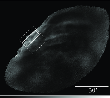
Figure 1: Band-ratio image of 1/4 keV band to 3/4 keV band at the northeastern region of the Cygnus Loop obtained with the ROSAT PSPC. White color represents enhanced 1/4 keV band emission. The dotted square shows the XIS field of view. The region extracted spectrum is shown by the white rectangular.

We retrieved the PSPC data (observation ID 500034) from the High Energy Astrophysics Science Archive Research Center Online Service, provided by the NASA/Goddard Space Flight Center. Figure 1 shows the image made by taking the ratio of flux in the 1/4 keV and 3/4 keV bands. As clearly shown in this image, there is significant spectral variation over the ROSAT field of view (FOV) in both the radial and azimuthal directions, with the very softest X-ray emission concentrated at the shock front. We thus extracted the Suzaku XIS spectrum from the region with the softest apparent X-ray emission (indicated by the white rectangular in figure 1). The size of this extraction region is 16.$\!{}^{\prime}$2$\times$5.$\!{}^{\prime}$9.

Figure 2 shows the extracted Suzaku XIS1 spectrum. Many emission lines are detected in the 0.2$-$1 keV region. To identify them, we fitted a parameterized spectral model consisting of 10 intrinsically narrow Gaussian functions with an underlying thermal bremsstrahlung continuum all absorbed by a photoelectric absorption function. The resultant best-fit emission line parameters and line identifications are summarized in table 1. We clearly detect line emission from highly-ionized C, N, and O. Based on this model fit, we calculate the line intensity ratios among different ionic species of N and O which enable us to estimate $kT_{\rm e}$ for the N and O emitting plasma. Assuming $kT_{\rm e}=0.13$ keV and collisional ionization equilibrium conditions, the strongest lines around 0.426 keV and 0.495 keV are N VI K$\alpha$ and N VII Ly$\alpha$, respectively, although there are also many emission lines from other elements present near these energies (ATOMDB ver 1.3.1; Smith et al. 2001). For comparison to the observed spectral results we use ATOMDB to calculate the intensity of all emission lines from all elements in the two energy bands: 0.48$-$0.51 keV and 0.41$-$0.44 keV, whose widths are intended to account, approximately, for the XIS energy resolution. Figure 3 shows the modeled line intensity ratio (0.48$-$0.51 keV band divided by 0.41$-$0.44 keV band) as a function of $kT_{\rm e}$. The two horizontal lines show the upper and lower limits for the observed intensity ratio between the 0.495 keV and 0.426 keV lines. Based on this figure, we find that the electron temperature of the plasma predominantly giving rise to the N emission is $kT_{\rm e}=0.127\pm 0.005$ keV which is consistent with that determined from the continuum emission (see table 1). We do a similar calculation for the energy bands around 0.564 eV and 0.653 eV. The bands used for the model calculations here, 0.63$-$0.67 keV and 0.54$-$0.58 keV, are dominated by emission from highly-ionized O and thus we only need to consider the O emission lines in ATOMDB. Figure 4 shows the modeled line intensity ratio. The electron temperature of the O-emitting plasma is $kT_{\rm e}=0.166\pm 0.001$ keV which is slightly higher than that of the continuum emission and N-emitting plasma. Given the significant dependence of the N and O line emissivities on temperature in this low $kT_{\rm e}$ regime, the results just presented suggest that there are at least two plasma components in this region.

We are thus led to investigate a two-component non-equilibrium ionization (NEI) model. We used Xspec ver 12.3 and the vnei NEI model (Borkowski et al. 2001) with the version number for the NEI models (NEIVERS) of 2.0. The free parameters are $kT_{\rm e}$, ionization timescale (log($n_{\rm e}t$) where $n_{\rm e}$ is the electron density and $t$ is the time since the plasma was shock heated), emission measure, the absorbing column density, $N_{\rm H}$, and the abundances of C, N, O, Ne, and Fe relative to their solar values (Anders & Grevesse 1989). The abundances of Mg, Si, S, Ar, and Ca were linked to that of Ne, while the Ni abundance was linked to Fe. $N_{\rm H}$ and abundances of the heavy elements were kept the same for both plasma components. The data are well reproduced by the vnei model as can been seen in figure 5, which plots the best-fit model in comparison to the spectral data. The best-fit parameter values are summarized in table 2. In paper I (see figure 5) there was extra scatter in the residuals plot associated with the emission lines, which has been greatly reduced in the present study thanks to our use of newer response matrix files that take into account the degradation of the XIS energy resolution.

The abundances of the heavy elements (with the exception of Si) are systematically larger than those presented in paper I. Updated calibration and response matrices files likely accounts for some of this discrepancy. The details of the model used for the fits differ as well. Here we use two NEI models with independent temperatures and ionization timescales, whereas before the ionization timescales were the same for the two plasma components. Another major difference is that here the abundances of Ne, Mg, Si, S, Ar, and Ca vary as a group with their relative abundances fixed at the solar values. In paper I the abundances of Ne, Mg, and Si varied freely, while Ar and Ca were fixed at their full solar values. It is important to note that the abundances we derive here for nearly all the heavy elements are $\sim$0.23, which means that their relative abundances are consistent with the solar values. This result strongly suggests that the soft X-ray emitting plasma is predominantly of interstellar origin. However, O stands out as being relatively depleted by a factor of two even though the O lines are among the strongest ones in this spectral range, as shown in table 1.

4 Discussion and Conclusion

We analyzed the very soft X-ray emission from the northeastern region of the Cygnus Loop with the Suzaku Observatory. The X-ray emitting plasma requires at least two spectral components; a high $kT_{\rm e}$ component with small ionization timescale and a low $kT_{\rm e}$ component with large ionization timescale.

Usually, X-ray emitting plasmas of SNRs are assumed to be optically thin because the typical density is quite low. Since the region we analyzed is very bright with a potentially large line-of-sight path length, however, this assumption may not be valid for some resonance lines. The line-center cross section of resonance scattering can be expressed as

$$\sigma={\sqrt{\pi}e^{2}\over mc}{f\over\nu}\left({v\over c}\right)^{-1}\simeq 1.86\times 10^{-9}\,{f\over E}\,v^{-1}\quad\mbox{cm}^{2}\ ,$$ (1)

where $f$ and $\nu$ are the oscillator strength and frequency, respectively, of the line transition concerned, $v$ is the root-mean-square kinetic velocity of the ion, $m$ is the electron mass and other quantities have their usual meanings. In the last expression, $E$ is the line energy in keV. The kinetic velocity is composed of thermal and turbulent motions, as

$$v^{2}=\left({2kT_{\rm i}\over m_{\rm i}}\right)^{2}+\xi^{2}\ ,$$ (2)

where $kT_{\rm i}$ is the ion temperature in keV, $m_{\rm i}$ is the ion mass, and $\xi$ represents the root-mean-square turbulent velocity due to motions other than thermal one. In the following analysis, we assume that the second term (turbulent motion) is negligibly small compared to the first one (thermal motion) in equation (2); the validity is discussed later.

The line-center optical depth for resonance scattering is given by

$$\tau=n_{z}\sigma L=\left({n_{z}\over n_{Z}}\right)\left({n_{Z}\over n_{\rm H}}\right)\left({n_{\rm H}\over n_{\rm e}}\right)\,n_{\rm e}\sigma L\ ,$$ (3)

where $L$ is the path length through the plasma, $n_{z}$ the ion density, $n_{Z}$ the element density, $n_{\rm H}$ the hydrogen density, and therefore $n_{z}/n_{Z}$ represents the ionic fraction, $n_{Z}/n_{\rm H}$ the elemental abundance relative to hydrogen. We assume $L=2.5$ pc and the emission volume to be 2.5$\times$0.93$\times$2.5 pc³. The electron density is obtained from the emission measure to be 1.25 and 1.35 cm^-3 for the high and low $kT_{\rm e}$ components, respectively, and $n_{\rm e}/n_{\rm H}$ is taken to be 1.2. For the ion temperature, we assume $kT_{\rm i}=kT_{\rm e}$ = 0.236 keV, which is the density-weighted mean value from table 2. In the calculation of $\sigma$ for the He-like K$\alpha$ lines, we summed the oscillator strengths for the three main lines of the He-like triplet, namely the forbidden ($z$), intercombination ($x+y$), and resonance ($w$) lines. The ionic fractions of O VII K$\alpha$ and O VIII K$\alpha$ were calculated by taking into account the NEI condition for each component separately (using Masai 1984). The density-weighted overall ionic fractions of O VII K$\alpha$ and O VIII K$\alpha$ were then determined to be 0.51 and 0.33, respectively. The inferred values of $\tau$ for O VII K$\alpha$ and O VIII K$\alpha$ turn out to be 0.54 and 0.16. Table 3 summarizes the resonance-line-scattering cross sections and optical depths for the K emission lines detected in the Suzaku data and shown in table 1. The optical depth of O VII K$\alpha$ is the largest whereas those of the other emission lines are not negligibly small.

In order to model the effect of self-absorption in a simple way, we employed the so-called “escape-factor” method (Irons 1979). We assume the global (source- and direction-average) Doppler-profile escape factor for plane-parallel “slab” geometry (Bhatia & Kastner 2000) which is a reasonable assumption for the shell-brightened appearance of the Cygnus Loop. Escape factor values for the relevant emission lines are summarized in table 3. All values are less than 0.87, indicating that our line intensities have been underestimated by a factor of 13% or more. Optical depth effects, therefore, play a significant role in the X-ray emission from the Cygnus Loop with the O abundance, in particular, being underestimated by a factor of 20–40%. However, optical depth effects alone cannot account for the entire abundance discrepancy of a factor of two that we observe. It should be noted as well that the escape factor is different for O VII K$\alpha$ and O VIII K$\alpha$, implying that the true line intensity ratio differs from the observed value. Correcting the line intensity ratio of O VIII K$\alpha$ to O VII K$\alpha$ for this effect results in a revised ratio of 0.21, which implies $kT_{\rm e}=0.15$ keV based on the APEC model of equilibrium ionization. This optical depth effect not only reduces derived elemental abundances but it also biases fitted $kT_{\rm e}$ measurements from their true values. Furthermore, varying the elemental abundance affects the calculation of the optical depth as shown in equation (3). Future work will be needed to develop more sophisticated emission codes that take optical depth effects into account.

We have made a few assumptions that tend to enhance the effects of resonance line scattering, including (a) temperature equipartition between electrons and ions, (b) no bulk motions, and (c) no turbulence. The temperature equipartition is a reasonable assumption for the region observed, as argued by Ghavamian et al. (2001) based on the optical spectra as well as by Miyata & Tsunemi (1999) on X-rays. Bulk motions may not be such a big problem for the Cygnus Loop due to its relatively low shock speed (few hundred km s^-1) and its large angular size on the sky. The region observed is right at the edge of the remnant’s rim and therefore can be approximated as a slab moving uniformly across the sky. This would not be the case if there was significant curvature of the remnant shell in the line of sight, or if we were viewing through the center of the remnant where the back part of the shell would be moving away from us while the front part was moving toward us. So the proximity of the Cygnus Loop to the Earth again favors resonance line scattering.

As for (c), very little information is available. One location where turbulence likely occurs is at the contact discontinuity of the ejecta in young SNRs. The instabilities that operate here drive turbulent eddies and vortices that imprint a random pattern of velocity flows onto the overall radial expansion of the ejecta. Any such turbulence has an effect of increasing the root-mean-square velocity broadening $v$ resulting in a reduction of the scattering cross section.

The forward shock in the adiabatic phase of remnant evolution is hydrodynamically stable and will not suffer this effect. But radiative cooling at the forward shock causes hydrodynamical instabilities (Blondin et al. 1998). Ultimately the amount of line broadening due to turbulence of this type will be some fraction of the shock velocity, so that younger SNRs will tend to have a higher line broadening and hence lower cross-section for resonance line scattering. If the part of the Cygnus Loop we observed is still in the Sedov phase of evolution, the conditions for minimal turbulence are met. Therefore, according to all three items discussed above, the Cygnus Loop is favored to have a significant effect due to resonance line scattering.

Since the Cygnus Loop appears to be a rim-brightened shell in the X-ray band, optical depth effects may only play an important role at the rim where the plasma path lengths are largest. The abundance of O relative to other heavy elements has been show to decrease at the shell region of the Cygnus Loop (e.g. Miyata & Tsunemi 1999). Likewise, Leahy (2004) analyzed Chandra data of the bright southwestern region and found that the abundances of O group elements (C, N, and O) is roughly half those of the Ne group (Ne, Na, Mg, Al, Si, S, and Ar) and Fe group (Ca, Fe, and Ni). The depleted O abundance relative to other elements is consistent with our results and suggests that optical depth effects might be important at the southwestern region too. It should be noted that Miyata & Tsunemi (1999) and Leahy (2004) assumed the C and N abundances relative to O to be solar because they had neither high enough spectral resolution nor sufficient effective area for detecting C and N lines. The Suzaku XIS camera enables us to determine the abundances of C, N, and O independently for diffuse X-ray sources so future additional observations with Suzaku are essential for abundance measurements. Katsuda et al. (2007) analyzed four Suzaku pointings of the northeastern region of the Cygnus Loop and showed that O is relatively depleted by a factor of two compared with other heavy elements. This result also supports our view for a significant optical depth effect. The Suzaku observatory has so far performed 8 mapping observations from the northeastern toward the southwestern region of the Cygnus Loop. Detailed analysis of the radial distribution of intensities of O VII K$\alpha$ and O VIII K$\alpha$ as well as their intensity ratios may help to clarify optical depth effects in the SNR. However, for this to work it will be necessary to separate out the effects of any intrinsic radial variation in the plasma temperature, which can also produce variations in the observed line intensity ratio.

In clusters of galaxies, an anomalous ratio of Fe K$\beta$ to K$\alpha$ emission lines has been observed, which is offered as evidence for resonance line scattering in the relatively dense central cluster plasma (e.g., Tawara 1995). Unfortunately, due to their NEI condition, the intensity ratio of the K$\beta$ to K$\alpha$ emission line complexes is not a good indicator of resonance line scattering in SNRs. For definitive answers, we need to resolve individual K-shell lines of He-like ions as well as the Ly$\alpha$ and Ly$\beta$ lines for a range of elemental species as a function of position across the extent of diffuse thermal X-ray sources. Hopefully in the near future X-ray microcalorimeters onboard $XEUS$, Con-X, and/or $NeXT$ will provide this capability and allow X-ray astronomers to use resonance scattering and other techniques to gain a deeper insight into the nature of SNRs.

We are grateful to all the other members of the Suzaku team. EM is supported by Grant-in-Aid for Specially Promoted Research (16002004) and the 21st Century COE Program, ‘Towards a new basic science: depth and synthesis’. JPH acknowledges support from NASA grant NNG05GP87G. This research has made use of data obtained through the High Energy Astrophysics Science Archive Research Center Online Service, provided by the NASA/Goddard Space Flight Center.

Table 1: Best-fit parameters of the Gaussian fitting.

Line energy (eV)	Intensity (photons s-1 cm-2)	Line identification
358$\pm$5	(3.0$\pm$0.1)$\times$10-2	C VI K$\alpha$
426$\pm$5	(1.1$\pm$0.1)$\times$10-2	N VI K$\alpha$
495$\pm$5	(3.9$\pm$0.2)$\times$10-3	N VII Ly$\alpha$, N VI K$\beta$
564$\pm$5	(3.20$\pm$0.05)$\times$10-2	O VII K$\alpha$
653$\pm$5	(8.7$\pm$0.1)$\times$10-3	O VIII Ly$\alpha$
722$\pm$5	(2.8$\pm$0.1)$\times$10-3	Fe XVII
792$\pm$6	(1.9$\pm$0.1)$\times$10-3	Fe XVII, Fe XVIII
837$\pm$7	(1.2$\pm$0.1)$\times$10-3	Fe XVII, O VIII Ly$\beta$
910$\pm$5	(2.01$\pm$0.06)$\times$10-3	Ne IX K$\alpha$
989$\pm$9	(2.6$\pm$0.7)$\times$10-4	Fe XVII, Ni XIX
Thermal bremsstrahlung	$kT_{\rm e}$ (keV)	0.13$\pm$0.01
Absorption	$N_{\rm H}$ ($\times 10^{20}$ cm-2)	1.9$\pm$0.2
$\chi^{2}$ (d.o.f.)∗	205 (195)

Errors quoted are 90% confidence level.
^∗ d.o.f. means degree of freedoms.

Table 2: Best-fit parameters of the vnei model fitting.

High $kT_{\rm e}$ component
$kT_{\rm e}$ (keV)	0.248${}^{+0.006}_{-0.001}$
log($n_{\rm e}t$)	10.6${}^{+0.02}_{-0.03}$
Emission measure∗ (cm-6pc3)	7.6$\pm$0.1
Low $kT_{\rm e}$ component
$kT_{\rm e}$ (keV)	0.224$\pm$0.001
log($n_{\rm e}t$)	11.98$\pm$0.06
Emission measure∗ (cm-6pc3)	8.8${}^{+1.9}_{-0.2}$
Element	Abundance
C	0.22$\pm$0.01
N	0.24$\pm$0.01
O	0.13$\pm$0.01
Ne,Mg,Si,S,Ar,Ca	0.23$\pm$0.01
Fe,Ni	0.24$\pm$0.01
$N_{\rm H}$ ($\times 10^{20}$ cm-2)	$<$ 2
$\chi^{2}$ (d.o.f.)	314 (204)

Errors quoted are 90% confidence level.
^∗ Emission measure is defined as $\int n_{\rm e}n_{\rm H}V$ where $n_{\rm H}$ is the Hydrogen density and $V$ is the emission volume.

Table 3: Cross section of resonance line scattering, optical depth, and escape factor for K emission lines detected.

Emission line identified	Cross section (10-16cm2)	Optical depth	Escape factor
C VI K$\alpha$	3.4	0.17	0.82
N VI K$\alpha$	6.0	0.11	0.87
O VII K$\alpha$	4.8	0.54	0.63
O VIII Ly$\alpha$	2.2	0.16	0.83
Ne IX K$\alpha$	3.3	0.17	0.82

Figure 2: Spectrum extracted from the softest region shown in figure 1. The best-fit curve of 10 Gaussian functions with the thermal bremsstrahlung model is shown by solid line. The contribution of each component is also shown by dotted line. Residuals between data and the best-fit model are shown in the lower panel.

Figure 3: Line intensity ratio of 0.48$-$0.51 keV band to 0.41$-$0.44 keV band. Two horizontal lines show the upper and lower limits for the intensity ratio of 0.495 eV line to 0.426 eV line.

Figure 4: Line intensity ratio of 0.63$-$0.67 keV band to 0.54$-$0.58 keV band. Two horizontal lines show the upper and lower limits for the intensity ratio of 0.653 eV line to 0.564 eV line.

Figure 5: Same as figure 2 but with the two component vnei model having different $kT_{\rm e}$ and different log($n_{\rm e}t$).

References

- [1] Anders, E., & Grevesse N. 1989, Geochim. Cosmochim. Acta, 53, 197
- [2] Bhatia, A.K. & Kastner, S.O., 2000, JQSRT, 67, 55
- [3] Blair, W.P., Sankrit, R., & Raymond, J.C. 2005, AJ, l29, 2268
- [4] Blondin, J.M. Wright, E.B. ,Borkowski, K.J. Reynolds, S.P., 1998, ApJ, 500, 342
- [5] Borkowski, K.J., Lyerly, W.J., & Reynolds, S.P. 2001, ApJ, 548, 820
- [6] Ghavamian, P., Raymond, J., Smith, C.R. & Hartigan, P. 2001, ApJ, 547, 995
- [Cornett et al.(1992)] Cornett, R. H., et al. 1992, ApJ, 395, L9
- [7] Irons, F.E., 1979, JQSRT, 22, 1
- [8] Ishisaki, Y. et al. 2007, PASJ, 59, S113
- [9] Kaastra, J.S. & Mewe, R. 1995, A&A, 302, L13
- [10] Katsuda, S., Tsunemi, H., Uchida, H., Miyata, E., Nemes, N., Miller, E.D., Mori, K., Hughes, J.P. 2007, PASJ, in press
- [11] Koyama, K. et al. 2007, PASJ, 59, S23
- [12] Leahy, D.A. 2004, MNRAS, 385, 351
- [13] Levenson, N.A. et al. 1997, ApJ, 484, 304
- [14] Masai, K. 1984, Ap&SS, 98, 367
- [15] Mitsuda, K. et al. 2007, PASJ, 59, S1
- [16] Miyata, E., Tsunemi, H., Pisarski, R., & Kissel, S.E. 1994, PASJ, 46, L101
- [17] Miyata, E., & Tsunemi, H. 1999, ApJ, 525, 305
- [18] Miyata, E., Katsuda, S., Tsunemi, H., Hughes, J.P., Kokubun, M., & Porter, F.S. 2007, PASJ, 59, S163 (Paper I)
- [19] Raymond, J.C., Black, J.H., Dupree, A.K., Hartmann, L., & Wolff, R.S. 1981, ApJ, 246, 100
- [Raymond et al.(1988)] Raymond, J. C., Hester, J. J., Cox, D., Blair, W. P., Fesen, R. A., & Gull, T. R. 1988, ApJ, 324, 869
- [20] Sankrit, R. & Wood, K. 2001, ApJ, 555, 532
- [21] Smith, R. et al. 2001, ApJ, 556, L91
- [22] Tawara, Y. 1995, in Proceedings of the 11th. col on UV and X-ray spectroscopy of astrophysical and laboratory plasmas, Nagoya