2MASS J01542930+0053266: A New Eclipsing M–dwarf Binary System

Abstract

We report on 2MASS J01542930+0053266, a faint eclipsing system composed of two M dwarfs. The variability of this system was originally discovered during a pilot study of the 2MASS Calibration Point Source Working Database. Additional photometry from the Sloan Digital Sky Survey yields an 8–passband lightcurve, from which we derive an orbital period of $2.6390157\pm 0.0000016$ days. Spectroscopic followup confirms our photometric classification of the system, which is likely composed of M0 and M1 dwarfs. Radial velocity measurements allow us to derive the masses (M${}_{1}=0.66\pm 0.03M_{\odot}$; M${}_{2}=0.62\pm 0.03M_{\odot}$) and radii (R${}_{1}=0.64\pm 0.08R_{\odot}$; R${}_{2}=0.61\pm 0.09R_{\odot}$) of the components, which are consistent with empirical mass–radius relationships for low–mass stars in binary systems. We perform Monte Carlo simulations of the lightcurves which allow us to uncover complicated degeneracies between the system parameters. Both stars show evidence of H$\alpha$ emission, something not common in early–type M dwarfs. This suggests that binarity may influence the magnetic activity properties of low-mass stars; activity in the binary may persist long after the dynamos in their isolated counterparts have decayed, yielding a new potential foreground of flaring activity for next generation variability surveys.

1 Introduction

Low–mass dwarfs ($0.07M_{\odot}\leq$ M${}_{\star}\leq 0.7M_{\odot}$) comprise $\sim$ 75% of all stars in the Milky Way, making them the most common luminous objects in the Galaxy (Reid et al., 1995). A significant amount of theoretical work has been devoted to constructing models that describe the physical processes in the interiors and atmospheres of these low–mass stars (e.g. Burrows et al., 1993; Baraffe et al., 1998; Hauschildt et al., 1999; Chabrier & Baraffe, 2000). Differences in the predictions of these models can be subtle, and distinguishing between them requires precise empirical constraints on fundamental stellar properties (mass, radius, luminosity, and effective temperature; Ribas, 2006). As low–mass stars are faint, small, and possess complex spectra dominated by strong molecular bands, measuring these parameters is challenging. Double–lined eclipsing binaries with detached, low–mass components of similar spectral type offer the best opportunity for accurate and precise measurements of these fundamental properties.

Although binary systems are more common than single stars at high stellar masses ($>$ 1 M_⊙; eg. Abt, 1983; Duquennoy et al., 1991), binaries are not very common in low–mass stars (Leinert et al., 1997; Reid & Gizis, 1997; Delfosse et al., 2004). In fact, the combination of low binary fraction and the sheer dominance (by number) of low–mass stars suggests that most of the stars in the Galaxy are actually single stars (Lada, 2006). Because of the low binary fractions and the faintness of M dwarfs, relatively few low–mass main sequence binaries have been studied (e.g. Creevey et al., 2005; López-Morales & Ribas, 2005; Hebb et al., 2006; Ribas, 2003, 2006; Blake et al., 2007, and references therein). Adding to the census of double–lined eclipsing binary systems is critical because they provide highly accurate, direct measurements of the masses and radii of the components, nearly independent of any model assumptions. While the known number of eclipsing low–mass binaries is small, next-generation variability and planet hunting surveys should increase the number of known systems.

Measurements of the masses and radii of the individual components of these low–mass systems have revealed potentially serious inadequacies in stellar evolution models (Ribas, 2003, 2006), whereas measurements and models agree for stars over $1M_{\odot}$. These discrepancies apparently extend down into the brown dwarf regime as evidenced by the first L–dwarf binary (Stassun et al., 2006, 2007). In particular, the mass-radius, mass-temperature, and mass-luminosity relationships predicted by stellar theory are inconsistent with a large fraction of observed M dwarf components (e.g. Hebb et al., 2006). Identifying and characterizing new low–mass eclipsing binaries will provide stronger constraints for theoretical models and help reveal the cause of the current discrepancies between observed and predicted properties of low–mass stars.

In this manuscript, we present the discovery of a new double-lined eclipsing binary system, 2MASS J01542930+0053266. In §2, we outline the photometric and spectroscopic observations of this binary system. Our determination of physical parameters and spectral types are detailed in §3. Discussion of the discrepancies between empirical and theoretical mass-radius relations is outlined in §4, followed by our conclusions in §5.

2 Observations

2.1 2MASS Photometry

The calibration observations of the Two Micron All Sky Survey (2MASS; Skrutskie et al., 2006) are a precursor to next–generation survey efforts such as LSST (Tyson, 2002). 2MASS observed the entire sky using three–channel cameras that simultaneously imaged in the $J$ (1.25 $\mu$m), $H$ (1.65 $\mu$m), and $K_{\rm s}$ (2.17 $\mu$m) passbands. To allow precision cross–calibration of the data, 35 $1\hbox{${}^{\circ}$}\times 8.\arcmin 5$ calibration fields were defined. An available calibration field was imaged approximately hourly over the duration of the survey. The total number of epochs obtained for a given calibration field ranges from 600 to 3700. The 2MASS Calibration Point Source Working Database (Cal-PSWDB) has recently been released as part of the 2MASS Extended Mission (Cutri et al., 2006), and contains a wealth of information on temporal variability (Plavchan et al., 2007; Becker & Cutri, 2008).

2MASS J01542930+0053266 (hereafter J0154) was first identified as a periodic variable in a pilot study of objects in 2MASS calibration region 90004, which was imaged 2977 times between July 1997 and November 2000. We extracted lightcurves for 5770 individual objects from the ensemble of data by clustering measurements taken at different epochs based on their celestial coordinates. For a given lightcurve, we used the 2MASS photometric quality flag $ph\_qual$ to reject poor–quality data points ($ph\_qual$ = D, E, F, or X). In total, 965 of these clipped lightcurves had more than 100 epochs. We phased all clipped lightcurves using a modified version of the Supersmoother algorithm (Riemann, 1994). For each object, the $J$, $H$, and $K_{\rm s}$ passbands were phased independently, and the best–fit periods were compared. The phasing of J0154 yielded periods of $1.31951246$ days in all three passbands (we note that Supersmoother converged upon an alias of the final period derived for this system). The composite colours of the system ($J-H=0.66$, $H-K=0.19$) suggest it consists of early–type dM stars (Covey et al., 2007).

2.2 SDSS Photometry

J0154 lies in the Sloan Digital Sky Survey’s (SDSS; Gunn et al., 1998; York et al., 2000; Stoughton et al., 2002; Pier et al., 2003; Gunn et al., 2006) Stripe 82, a $\sim$ 300 sq. deg. equatorial region that has been imaged repeatedly over the course of the SDSS. Stripe 82 is imaged by the SDSS–II Supernova Survey every other night from September to December, 2005–2007 (Frieman et al., 2008). The extensive repeat imaging of this region of sky has enabled precise photometric and astrometric calibration of this Stripe, yielding the Stripe 82 Light-Motion Curve Catalogue (LMCC; Bramich et al., 2008). We extracted the light–motion curve for J0154 from the LMCC, which consists of 32 $u,g,r,i$ and $z$–band (Fukugita et al., 1996; Smith et al., 2002) measurements of the system, including SDSS–I observations as far back as Sept, 1998 and up to the end of SDSS–II supernova survey observations in Dec, 2005. The catalogue reports a proper motion vector for the system of $\mu_{\alpha}$ = $0.88\pm 2.25$ mas yr^-1 and $\mu_{\delta}=-11.19\pm 2.25$ mas yr^-1.

Figure 1 displays the ensemble lightcurve, folded at the best–fit period of 2.6390157 days. The lightcurves are ordered from top to bottom and left to right $K_{\rm s},H,J,z,i,r,g,u$. The $J$, $H$, and $K_{\rm s}$ data are binned every 30 points. We note that SDSS has no data during the secondary eclipse, resulting in poorly constrained relative optical colours for each star. This system is one of the faintest known eclipsing low–mass systems ($r=18.3$), meaning substantial telescope time is required to measure the radial velocity curve to high precision.

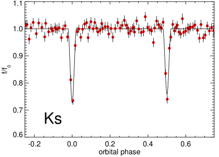
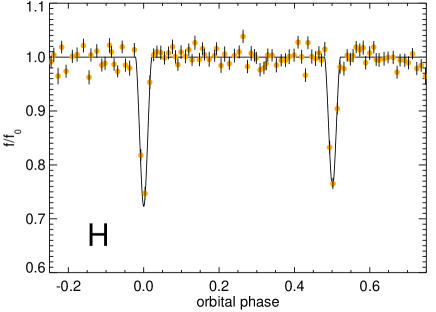
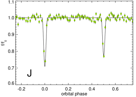
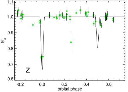
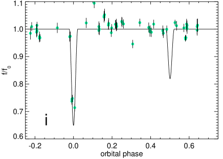
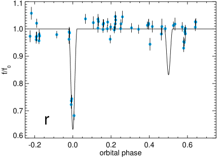
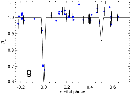
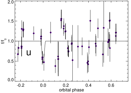
Figure 1: Lightcurve of J0154 folded at the best–fit period of 2.6390157 days, with J, H and Ks binned every 30 points for clarity.

2.3 Spectroscopy

2.3.1 Apache Point Observatory

To confirm our M–dwarf classification, we obtained spectroscopic observations of this system using the ARC 3.5-m telescope with the Dual-Imaging Spectrograph (DIS-III) at Apache Point Observatory (APO) on the nights of 2005 November 22, 2005 November 28, and 2005 December 04 UT. We used the HIGH resolution gratings (0.84Å/pixel in the red; 0.62Å/pixel in the blue) and a $1.\arcsec 5$ slit centered at 6800Å (red) and 4600Å (blue). The chips were binned 2$\times$1 to increase the signal-to-noise and windowed from their original size of 2048k$\times$2048k to reduce the readout time between exposures. The approximate wavelength coverage is $\sim 1000$Å in both the red and blue wavelength regions.

The spectroscopic reductions were performed using standard $IRAF$ reduction procedures. The calibration images (bias, flat, arc, flux) used to correct each of the individual spectra were applied only to images taken on the same night. The bias, and flat images were observed at the beginning or end of each night. A He–Ne–Ar arc lamp spectrum was taken after each exposure on the target star.

A representative spectrum of J0154 is displayed in Figure 2. These initial spectra clearly demonstrate the features of an M–dwarf system. The presence of H$\alpha$ in emission at 6563 Å indicates magnetic activity, although no obvious line splitting is detected. The broad molecular bands of TiO ($\sim 7050$ Å) are also readily apparent.

Figure 2: Spectrum of J0154 obtained on the ARC 3.5-m telescope with the DIS-III spectrograph (0.84Å/pixel) on 2005 November 22 UT. Note the H$\alpha$ emission near 6563 Å, indicating chromospheric activity.

2.3.2 Magellan

Two 600 second exposures of J0154 were obtained with the Low Dispersion Survey Spectrograph 3 (LDSS3) on the Magellan II/Clay telescope on the night of December 29, 2005. The VPH Blue grating (0.682 Å/pixel; R = 1900) and a $2\arcsec$ slit were used. The spectra were reduced and calibrated employing standard techniques, which include subtracting a combined bias, subtracting the overscan correction, flat-fielding with quartz lamp observations, cleaning the image of cosmic rays, and extracting a region centered on the target star. The dispersion solution was derived from an observation of a He–Ne–Ar arc lamp. Flux calibrations were derived from observations of spectrophotometric standard stars from Oke & Gunn (1983). The spectra were corrected for the continuum atmospheric extinction using mean extinction curves. Telluric lines were removed using a procedure similar to that of Wade & Horne (1988) and Bessell (1999). We use the Magellan spectra to estimate the spectral types of the components in Section 3.2.1.

2.3.3 Keck

We were unable to resolve line splitting in either the APO or Magellan spectra, and therefore made use of the HIRES spectrograph at Keck during observing runs on 2006 October 13, 2006 December 12 and 2007 January 6. Over the 3 nights we obtained five spectra at R$\sim$50,000 with exposure times ranging from 30-40 minutes each.

The data were reduced using standard IDL routines that included order extraction, sky subtraction, and cosmic ray removal. The resulting S/N per pixel (0.06 Å/pixel) ranged from 6-9. The detection of H$\alpha$ emission lines in both stars due to magnetic activity allowed measurement of their radial velocities (we were unable to use cross correlation techniques on the lower resolution APO and Magellan spectra). An illustrative example of the Keck data is shown in Figure 3. The H$\alpha$ emission lines were fit to a double Gaussian profile using Levenberg–Marquardt least–squares minimization. Epochs and radial velocities for each of the 5 observations can be found in Table 1. The radial velocity curve derived from these data is shown in Figure 4.

Figure 3: Spectrum of J0154 obtained with HIRES (0.06 Å/pixel) on the Keck 10-m telescope on Oct 13, 2006. Note the line splitting around H$\alpha$ at 6563 Å, yielding emission peaks centered near 6561.5 Å and 6564.9 Å.

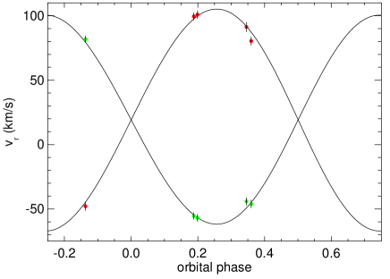
Figure 4: Radial velocity curve derived from the Keck data. The system velocity is $19.1\pm 1.3$ km s^-1. Velocities are relative to the solar system barycenter.

3 Analysis

3.1 Modeling The System

We corrected the times of all observations, as well as measured radial velocities, to the solar system barycenter (TDB). We analyzed the lightcurve of J0154 using the code of Mandel & Agol (2002). All of the orbital elements of the binary were allowed to vary, and we allowed the masses and radial velocity of the center of mass of the system to vary simultaneously while fitting the parameters describing the lightcurve. As both stars are well within their Roche radii and the centripetal acceleration at the equator is three orders of magnitude smaller than the surface gravity, we treated each star as a sphere (and hence ignore gravity darkening). Also, the stars are sufficiently separated that we can ignore reflected light. The one uncertainty in our models is the limb-darkening, which should be modest in the infrared (Claret et al., 1995). We find that the assumed limb-darkening affects our results very little, so we fix the linear limb-darkening coefficients for each star, $u_{1,2}$, at the values computed by Claret (2000, 2004) for model atmospheres with $T_{eff}=3800$ and $3600$ for the primary and secondary, respectively. We assume $log(g)=4.5$, $[M/H]=0$, and a microturbulent velocity of $2$ km s^-1 for both, based on the PHOENIX atmosphere models of Hauschildt et al. (1999). The limb-darkening parameters are given in Table 2.

Our model contains 25 free parameters, starting with the five orbital parameters: the eccentricity and longitude of pericenter combine to two parameters, $e\cos{\omega}$ and $e\sin{\omega}$; the inclination, $i$; the time of primary eclipse $T_{0}$ (which can be translated into a time of periapse); and the period, $P$ (which can be translated into a semi–major axis from the total mass of the system). Four parameters describe the bulk stellar properties: $R_{1}$, $R_{2}$, $M_{1}$, and $M_{2}$. The radial velocity of the center of mass of the system is $\gamma$ (in km s^-1). The fluxes are described by 15 parameters (we hold the $u$-band flux of the second star fixed at zero as the best–fit value is negative). For the model fitting, we transformed to the set of parameters suggested by Tamuz et al. (2006) which have weaker correlations between the transformed parameters. We found the initial best–fit model using Levenberg–Marquardt least–squares non–linear optimization giving a best-fit model with $\chi^{2}=11304.4$ for 9168 degrees of freedom. We found that the scatter of the data outside of eclipse had a gaussian shape, but with a larger scatter than the errors would warrant. It is possible that this discrepancy is due to variability in the stellar fluxes as the data were gathered over several years, or that the error bars are simply underestimated, so we added a systematic error in quadrature ($0.04,0.03,0.03,0.01,0.02,0.02,0.01,0.26$ magnitudes in the $K_{\rm s},H,J,z,i,r,g,u$–bands, respectively) such that the reduced $\chi^{2}$ of the data outside of eclipse in each band is equal to unity, and then refit the entire data set. The resulting $\chi^{2}$ of 9253.2 has a formal probability $P(\chi^{2}>9253.2)=$26% for 9168 degrees of freedom. The best fit parameters for the brightness of the system are given in Table 2 and the orbital and physical parameters in Table 3.

As the number of free parameters is large and the parameters can be strongly correlated, we ran simulated data sets, adding gaussian noise to the best-fit lightcurve and radial velocity model values. We ran $10^{5}$ simulations, and for each simulation re-ran the fitting routine to derive the best-fit parameters from the simulated data. We used the $10^{5}$ sets of derived parameters simulations to compute the 1-$\sigma$ errors on the best-fit model parameters, sorting each parameter and choosing the 68.3% confidence intervals, which are given in Tables 2 and 3. We computed a 90% confidence upper limits on the $u$ band flux of Star 2 by increasing its value from zero, while minimizing over the other system parameters, until the change in chi-square was $\Delta\chi^{2}=2.71$. Our analysis yields asymmetric error bars for all system parameters. We quote a single error bar when the negative and positive uncertainties are the same to within $10\%$.

The best–fit lightcurve is shown in Figure 1. The total flux of the two stars is very well constrained due to the large number of data points of high photometric quality. However, the individual fluxes are more poorly constrained due to the small number of points taken during the eclipses, so that uncertainties in the radius, limb-darkening, and inclination lead to uncertainties in what fraction of each total stellar flux is obscured during primary and secondary eclipse. Thus the derived fluxes of each star are strongly anti-correlated, which is why the errors on the individual fluxes are much larger than the error on the total flux (Table 2). The fit indicates that, in the infrared passbands, the eclipses are of very similar depths (0.35 vs 0.31 magnitudes in the $Ks$–band), which is the reason that the original Supersmoother fit converged on an alias of half the period.

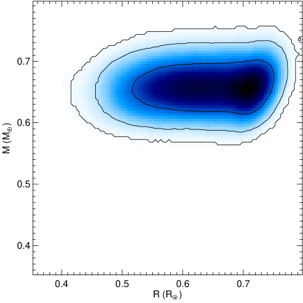
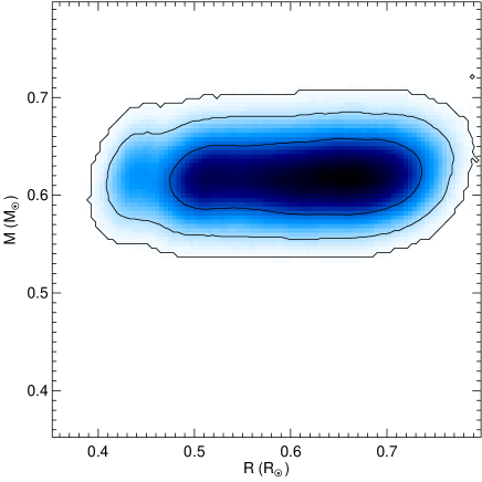
Figure 5: Mass–radius parameter space allowed by our data on J0154. The left figure is for the heavier (primary) object, while the right figure is for the secondary. The shaded area correspond to the probability distribution derived from the simulated data sets, while the contours represent the 1-,2-, and 3-sigma confidence regions.

The allowed mass–radius parameter space for each star is shown in Figure 5. Each panel shows the probability distribution of the mass and radius of each star derived from the simulated data sets in units of solar radius and mass. The contours are 1-,2-, and 3-sigma confidence regions (68.3%, 95.4%, and 99.73% of the $10^{5}$ parameter sets). We compare the derived values to the masses and radii found for other low–mass stars in Section 4.1.

From our results, we can derive several auxiliary parameters for the stars which have different error bars than if they are computed from the parameters in Table 3 due to covariance between model parameters. We also list in Table 3 (below the horizontal line) : the mass-radius ratio for each star, $M_{1,2}/R_{1,2}$; the ratio of the radii of the two stars, $R_{1}/R_{2}$; the sum of the stellar radii, $R_{1}+R_{2}$; the ratios of the semi-major axis to the stellar radii, $a/R_{1,2}$; the velocity semi-amplitudes, $K_{1,2}$ and the total amplitude $K$; the surface gravities, $log(g_{1,2})$; the stellar densities $\rho_{1,2}$; and the total mass of the system, $M_{1}+M_{2}$, which can be used to derive a semi-major axis of the system, $a$. At mid-eclipse, the projected separation of the stellar centers on the sky is $b$. The fractional error on $(R_{1}+R_{2})/a$ is much smaller ($\sim 2$%) than on $R_{1}$ or $R_{2}$ individually ($>10$%) due to strong correlations between $R_{1}/a$, $R_{2}/a$ and $i$, as discussed by Tamuz et al. (2006). Since our derived fluxes of the stars cover the peak in their spectral energy distributions, we have derived the bolometric flux ratio of the stars by smoothly interpolating between the fluxes in the different bands, and then taking the ratio of the two stars. Given the relative sizes and fluxes of the stars, we derive the ratio of the effective temperatures, $T_{2}/T_{1}$ (we cannot derive the absolute fluxes or effective temperatures from the lightcurve and RV data as we do not know the distance to this system to high precision).

3.2 Spectral Types and Temperature Estimates

While the masses, radii and fluxes for each star are well-determined by our modeling procedure, there are other quantities that can be measured from our observations. The spectral types of each component, total space velocity of the system and effective temperature estimates can be determined from our assembled dataset.

3.2.1 Binary Spectral Template Matching

In order to estimate the spectral types of this composite system, we constructed a grid of binary spectral templates. The spectra employed in synthesizing the binary templates were drawn from the low–mass stellar templates of Bochanski et al. (2007) and the K5 and K7 templates used in the HAMMER spectral analysis software package (Covey et al., 2007). Each template spectrum was scaled by its bolometric luminosity (Reid & Hawley, 2005) and coadded with all other templates. Relative velocity shifts were introduced for each spectral type pair, ranging from -200 km s^-1 to 200 km s^-1 in steps of 20 km s^-1. The final binary spectra grid consisted of 1638 templates. The templates were normalized to the Magellan observations and residuals were computed from 4500 to 7000 Å. The best fit binary pair for the Magellan spectra is an M0 primary and M1 secondary, with an uncertainty of $\pm 1$ subtype for each component. We did not use the velocity information as a constraint, but rather included the relative shifts for completeness. We adopt these subtypes for each component. The best fit composite spectrum is shown in Figure 6, along with the Magellan data.

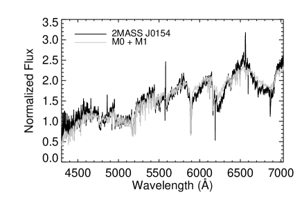
Figure 6: Magellan spectra (0.682 Å/pixel) of J0154 along with the best fit binary spectral template. The best fit binary template is composed of an M0 + M1.

3.2.2 Spectral Types From Optical–IR Colours

Using the colour–spectral type relationships for $r-i$, $i-z$, and $i-J$ derived by West et al. (2005) and Bochanski et al. (2007), we estimate a spectral type of M0 ($\pm$ 1 subtype) for the primary and M3 for the secondary. The intrinsic spread in colour at a given spectral type and our measured errors permit a range of spectral types between M0 and M4 for the secondary. Because of this large uncertainty, we adopt the secondary subtype derived from the spectral template analysis, and note that these colour–based results are consistent with the spectroscopic results derived in Section 3.2.1. We estimate a distance of $623\pm 50$ pc from the $i$–band photometric parallax (West et al., 2005) of the primary star. At a Galactic latitude of $b$ = $-58\hbox{${}^{\circ}$}$, this binary has vertical distance below the Disk of $\sim 530$ pc, consistent with being a member of the Galactic thin disk.

The thin disk membership of J0154 is strengthened by examining the system’s kinematics. The tangential velocity implied by the observed proper motion ($11.2\pm 3.2$ mas year^-1) and distance to the system is $33.1\pm 12.1$ km s^-1. Added in quadrature with the system radial velocity from the binary fit, we find a space velocity of $38.2\pm 12.2$ km s^-1, again consistent with the thin disk (Bochanski et al., 2007).

3.2.3 Metallicity and Temperature Estimates

We measured the composite CaH2, CaH3, and TiO5 molecular indices in our APO spectra of this system, and find CaH2 = $0.64\pm 0.06$, CaH3 = $0.83\pm 0.03$, and TiO5 = $0.64\pm 0.04$. Using these values along with the empirical formula from Figure 2 of Woolf & Wallerstein (2006) yields an effective temperature estimate for the primary of $T_{\rm eff}=3730\pm 100K$, consistent with the M0 spectral type determined from the full spectra. Further, when these measurements are compared with the samples of Lépine et al. (2003), Woolf & Wallerstein (2006), Burgasser & Kirkpatrick (2006), and West et al. (2008), they suggest that the composite system is of solar or slightly super–solar metallicity, again consistent with thin disk membership.

4 Discussion

Previous studies (e.g. Ribas, 2006, and references therein), have demonstrated that current models underpredict the radii of low–mass stars at a given mass. The radii derived for J0154’s components (R${}_{1}=0.64\pm 0.08R_{\odot}$ at M${}_{1}=0.66\pm 0.03M_{\odot}$, R${}_{2}=0.61\pm 0.09R_{\odot}$ at M${}_{2}=0.62\pm 0.03M_{\odot}$) lie in between different model predictions, and the errors are currently large enough to not yet provide discrimination between the models. The source of the uncertainties on the stellar radii is almost entirely due to the large errors on the photometry given the faintness of this system. A severe banana-shaped degeneracy between the impact-parameter (or inclination) and the ratio of the stellar radii occurs due to the large photometric errors (Figure 7); this is why in Table 3 the fractional error on $R_{1}+R_{2}$ ($\sim$ 3%) is much smaller than the fractional error on $R_{2}/R_{1}$ ($\sim$ 30%). Within the 68.3% confidence limit, the deviation of the K-band lightcurve from the best-fit lightcurve is only 0.6%, which implies that milli-magnitude precision would be required to derive the radius ratio to high accuracy. Below, we discuss the implications of our system with regards to current theoretical and empirical mass-radius relations.

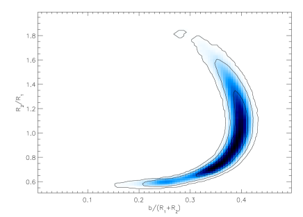
Figure 7: Confidence limits on $b/(R_{1}+R_{2})$ and $R_{2}/R_{1}$ from the synthetic data sets. The shaded region shows the density of points from the best-fit parameters to $10^{5}$ simulated data sets, while the contours are 68.3%, 95.4%, and 99.73% confidence regions.

4.1 The Empirical Mass–Radius Relationship

In Figure  8, the masses and radii of known low–mass eclipsing binary systems (López-Morales, 2007; Lopez-Morales et al., 2006; López-Morales & Shaw, 2007) are plotted along with current empirical (Bayless & Orosz, 2006) and theoretical models (Baraffe et al., 1998; Siess et al., 2000). Bayless & Orosz (2006) have derived an empirical mass–radius relationship for K and M dwarfs from known binaries that stretches up to nearly $0.8M_{\odot}$. We test this empirical mass-radius relation by comparing their expected radii, given our mass measurements, to our measured radii. Their analysis predicts $R_{1}=0.67\pm 0.03R_{\odot}$ and $R_{2}=0.63\pm 0.03R_{\odot}$, while we measure $R_{1}=0.64\pm 0.08R_{\odot}$ and $R_{2}=0.61\pm 0.09R_{\odot}$. Our objects are consistent with the ensemble of eclipsing binary stars used to derive their relationship, and fill in the gap at the high–mass, early–dM end of the relationship. The dearth of data in Figure 8 and the recent discovery of many of these systems reflects that this is an emerging field, only recently enabled by large–scale photometric surveys.

Theoretical models predict mass-radius relations which are a strong functions of both metallicity and age (Baraffe & Chabrier, 1996). The predictions of the Baraffe et al. (1998) evolutionary models for objects of solar metallicity and ages of $10^{8}-10^{9}$ years are consistent with J0154, yet disagree with other systems of similar mass. The models tend to systematically underpredict the radii at a given mass, as shown in Figure 8. While the uncertainties on the masses and radii of J0154’s components render them an equally good fit to both the Baraffe et al. (1998) theoretical models and Bayless & Orosz (2006) empirical fit, additional photometric and spectroscopic data should yield more precise measurements of these attributes, and better discrimination between models.

For comparison, the models of Siess et al. (2000) are also shown in Figure 8. The large differences between models with similar inputs for metallicity and age highlight the uncertainty that presently exists in this field. Hopefully this situation will be remedied by more high-precision measurements of fundamental stellar parameters in binary systems, along with updated models.

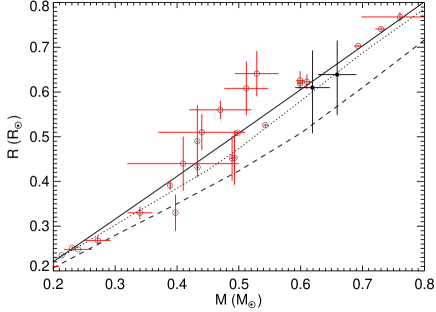
Figure 8: Distribution of mass vs. radius for known low–mass double–lined eclipsing binary systems (open circles; López-Morales 2007; López-Morales et al. 2006; López-Morales & Shaw 2007; Maxted et al. 2004). The solid line shows an empirical relationship derived by Bayless & Orosz (2006); the dotted line represents the Z=0.02, Y=0.275, T=1 Gyr models of Baraffe et al. (1998); the dashed line represents the Z=0.02, Y=0.28, T=1 Gyr models of Siess et al. (2000). The solid dots correspond to the components of J0154.

4.2 Activity

An interesting aspect of this system is the observed H$\alpha$ emission in both of the components. West et al. (2004) find that less than 5% of isolated M0 and M1 stars show activity (H$\alpha$ equivalent width of at least 1Å). The activity in early-type M dwarfs is also short lived ($<$ 1 Gyr; Hawley et al., 2000; West et al., 2008). It would be very unlikely to randomly draw an active M0 and M1 star from the field population, suggesting that some aspect of the interactions between the components is inducing the observed magnetic activity. The improbability of the stars being independently active is furthered when we consider the distance that this pair is from the Galactic plane. It is likely that M0 and M1 dwarfs that are several hundred pc from the Plane have been dynamically heated for many Gyrs and have ceased being active (West et al., 2008).

A search through the Palomar/MSU Nearby Star Catalog of Gizis et al. (2002) shows that a large fraction (20/22) of double–lined spectroscopic M–dwarf binaries have magnetically active components (H$\alpha$ equivalent width of at least 1Å). Other empirical studies (e.g. López-Morales, 2007) have suggested that the magnetic activity and metallicity of a star may affect its radius, drawing an explicit connection between the enhanced activity and large radii found in M–dwarfs in binary systems. Chabrier et al. (2007) suggest that enhanced magnetic activity may lead to inefficient thermal transport in stellar interiors. This results in objects with larger radii and smaller effective temperatures than stars where magnetic effects are negligible. Rapid stellar rotation may similarly affect the interior convection. In addition, enhanced surface spot coverage ($30-50\%$), due to strong magnetic activity, may impact the stellar radius. Either of these effects may be responsible for the empirical mass–radius relationships found in low–mass binary stars; additional data are required to constrain these theories.

5 Conclusions

We report the discovery and characterization of the double–lined eclipsing binary system 2MASS J01542930+0053266. Photometric and spectroscopic evidence suggests that both components are M dwarfs, and we adopt classifications of M0 and M1 as their subtypes. We resolve splitting of the H$\alpha$ emission line with spectroscopic observations using HIRES at Keck, leading to a radial velocity curve and estimates of the masses and radii of each star. Simulated data sets created by adding noise to the best fit provides uncertainties on and covariances between the system parameters. We emphasize that there exist complicated degeneracies between parameters in eclipsing systems that can only be fully explored with such detailed analyses.

Our analysis is consistent with previous studies of double–lined eclipsing M–dwarf systems. An empirical study by Bayless & Orosz (2006) yields a quadratic mass–radius relationship spanning the range of $0.2-0.8M_{\odot}$ and spectral types from late K to late M. This empirical relation accurately predicts the radii of J0154’s components.

We observe H$\alpha$ emission from both components, an unlikely scenario given their early–M spectral types and their distance from the Galactic plane. If magnetic activity is enhanced in M dwarfs in binary systems, the binary population including M–dwarfs components may present an additional foreground of stellar flares for next generation time domain surveys (Kulkarni & Rau, 2006; Becker et al., 2004).

Table 1: Radial Velocities

Date (TDB)	$v_{1}$ (km s-1)	$v_{2}$ (km s-1)
54021.3758	$-55.49\pm 2.75$	$99.51\pm 2.95$
54021.4043	$-57.00\pm 2.89$	$100.90\pm 3.25$
54081.2152	$81.77\pm 2.80$	$-47.93\pm 3.45$
54106.2401	$-41.12\pm 3.06$	$91.28\pm 3.74$
54106.2778	$-46.12\pm 3.12$	$80.38\pm 3.38$

Barycentric radial velocities measured from the Keck data on Oct 13, 2006, Dec 12, 2006 and Jan 6, 2007. The errors include a systematic error of 1.75 km s^-1 which has been added in quadrature to each of the measured velocity uncertainties. Dates are in Modified Julian Day (MJD) corrected to the solar system dynamic barycenter (TDB).

Table 2: Apparent brightness, colours, and limb-darkening of J0154

Filter	Star 1	Star 2	Total	$f_{2}/f_{1}$	$m_{1}-K_{\rm s,1}$	$m_{2}-K_{\rm s,2}$	$m_{tot}-K_{\rm s,tot}$	$u_{1}$	$u_{2}$
$u$	$21.95\pm 0.05$	$>22.74^{a}$	$21.9477\pm 0.0461$	$<0.95^{a}$	$6.67^{+0.247}_{-0.323}$	$>7.2^{a}$	$7.3047\pm 0.0462$	0.713	0.734
$g$	$19.89^{+0.32}_{-0.23}$	$21.26^{+1.22}_{-0.72}$	$19.6159\pm 0.0038$	$0.2833^{+0.43}_{-0.25}$	$4.61^{+0.072}_{-0.057}$	$5.73^{+0.875}_{-0.419}$	$4.9729\pm 0.0043$	0.829	0.814
$r$	$18.59^{+0.32}_{-0.23}$	$19.70^{+1.06}_{-0.59}$	$18.2573\pm 0.0039$	$0.3581^{+0.46}_{-0.26}$	$3.31\pm 0.07$	$4.18^{+0.670}_{-0.303}$	$3.6143\pm 0.0043$	0.808	0.777
$i$	$17.69^{+0.32}_{-0.23}$	$18.66^{+0.91}_{-0.52}$	$17.3164\pm 0.0035$	$0.4100^{+0.48}_{-0.27}$	$2.41\pm 0.07$	$3.13^{+0.505}_{-0.238}$	$2.6734\pm 0.0041$	0.696	0.672
$z$	$17.22^{+0.31}_{-0.23}$	$17.99^{+0.69}_{-0.44}$	$16.7874\pm 0.0032$	$0.4943^{+0.50}_{-0.28}$	$1.94\pm 0.06$	$2.46^{+0.298}_{-0.167}$	$2.1444\pm 0.0038$	0.611	0.589
$J$	$16.08^{+0.29}_{-0.22}$	$16.47^{+0.42}_{-0.32}$	$15.5019\pm 0.0013$	$0.6979^{+0.53}_{-0.31}$	$0.80\pm 0.05$	$0.94\pm 0.06$	$0.8589\pm 0.0024$	0.481	0.428
$H$	$15.46^{+0.31}_{-0.23}$	$15.74^{+0.41}_{-0.30}$	$14.8373\pm 0.0015$	$0.7672^{+0.58}_{-0.34}$	$0.18\pm 0.05$	$0.22\pm 0.06$	$0.1943\pm 0.0025$	0.453	0.398
$K_{\rm s}$	$15.28^{+0.31}_{-0.24}$	$15.53^{+0.40}_{-0.30}$	$14.6430\pm 0.0020$	$0.7971^{+0.60}_{-0.36}$	–	–	–	0.377	0.329

a : In the $u$ band the best-fit flux for the second star is zero, so we report 90% limits on the magnitude and colours of this star.

The apparent brightnesses of each component of J0154, as well as the composite system brightness, as derived from our global fit. We also list the adopted limb–darkening parameters $u_{1,2}$ for the components (Claret, 2000, 2004). The total system brightness is better constrained than those of the individual components because of the latter’s covariance with the radii of the stars, as well as the inclination of the system. Due to the anticorrelation between the fluxes of the two stars, the flux ratio (column 5) has larger uncertainties. The colours have smaller errors than the magnitudes since the fluxes in each band are strongly correlated for each star. We quote a single error bar when the positive and negative uncertainties are the same to within 10%.

Table 3: Binary Fit Parameters

Parameter	Value
$e$ cos($\omega$)	$0.00142\pm 0.00068$
$i$ (radians)	$1.51445_{-0.00109}^{+0.00839}$
$e$ sin($\omega$)	$-0.006\pm 0.012$
$T_{\rm 0}$ (TDB)	$52244.82052\pm 0.00058$
$P$ (days)	$2.6390157\pm 0.0000016$
$R_{1}$($R_{\odot}$)	$0.639_{-0.090}^{+0.076}$
$R_{2}$($R_{\odot}$)	$0.610_{-0.102}^{+0.083}$
$M_{1}$($M_{\odot}$)	$0.659\pm 0.031$
$M_{2}$($M_{\odot}$)	$0.619\pm 0.028$
$\gamma$ (km s-1)	$19.09\pm 1.28$
$M_{1}/R_{1}$($M_{\odot}/R_{\odot}$)	$1.032^{+0.171}_{-0.112}$
$M_{2}/R_{2}$($M_{\odot}/R_{\odot}$)	$1.016^{+0.204}_{-0.124}$
$R_{1}+R_{2}$ ($R_{\odot}$)	$1.248^{+0.021}_{-0.048}$
$R_{2}/R_{1}$	$0.955^{+0.304}_{-0.244}$
$a/R_{1}$	$13.652^{+2.220}_{-1.455}$
$a/R_{2}$	$14.299^{+2.850}_{-1.707}$
$K_{1}$ (km s-1)	$80.896\pm 1.811$
$K_{2}$ (km s-1)	$76.062\pm 4.204$
$K$ (km s-1)	$156.959\pm 5.901$
$log(g_{1}$ [cm s-2])	$4.646^{+0.131}_{-0.098}$
$log(g_{2}$ [cm s-2])	$4.659^{+0.158}_{-0.111}$
$\rho_{1}$ (g cm-3)	$3.563^{+2.032}_{-1.023}$
$\rho_{2}$ (g cm-3)	$3.849^{+2.790}_{-1.223}$
$M_{1}+M_{2}$ ($M_{\odot}$)	$1.278\pm 0.054$
$M_{2}/M_{1}$	$0.940\pm 0.034$
$a$ ($R_{\odot}$)	$8.718\pm 0.123$
$a$ (AU)	$0.041\pm 0.001$
$b$ ($R_{\odot}$)	$0.396^{+0.005}_{-0.050}$
$T_{2}/T_{1}$	$0.947^{+.032}_{.016}$

Best fit system and physical parameters of J0154 (above line) and derived parameters (below line). The fitting process is described in Section 3.1. Uncertainties in the parameters are derived from the distribution of best-fit values for the 10⁵ synthetic light curves. We quote a single error bar when the positive and negative uncertainties are the same to within 10%.

References

- Abt (1983) Abt H. A., 1983, ARA&A, 21, 343
- Baraffe & Chabrier (1996) Baraffe I., Chabrier G., 1996, ApJ, 461, L51+
- Baraffe et al. (1998) Baraffe I., et al. 1998, A&A, 337, 403
- Bayless & Orosz (2006) Bayless A. J., Orosz J. A., 2006, ApJ, 651, 1155
- Becker & Cutri (2008) Becker A. C., Cutri R. M., 2008, In preparation
- Becker et al. (2004) Becker A. C., et al. 2004, ApJ, 611, 418
- Bessell (1999) Bessell M. S., 1999, PASP, 111, 1426
- Blake et al. (2007) Blake C. H., et al. 2007, ArXiv e-prints, 707
- Bochanski et al. (2007) Bochanski J. J., et al. 2007, AJ, 134, 2418
- Bochanski et al. (2007) Bochanski J. J., et al. 2007, AJ, 133, 531
- Bramich et al. (2008) Bramich D., et al. 2008, In preparation
- Burgasser & Kirkpatrick (2006) Burgasser A. J., Kirkpatrick J. D., 2006, ApJ, 645, 1485
- Burrows et al. (1993) Burrows A., et al. 1993, ApJ, 406, 158
- Chabrier & Baraffe (2000) Chabrier G., Baraffe I., 2000, ARA&A, 38, 337
- Chabrier et al. (2007) Chabrier G., Gallardo J., Baraffe I., 2007, A&A, 472, L17
- Claret (2000) Claret A., 2000, A&A, 363, 1081
- Claret (2004) Claret A., 2004, A&A, 428, 1001
- Claret et al. (1995) Claret A., Diaz-Cordoves J., Gimenez A., 1995, A&AS, 114, 247
- Covey et al. (2007) Covey K. R., et al. 2007, AJ, 134, 2398
- Creevey et al. (2005) Creevey O. L., et al. 2005, ApJ, 625, L127
- Cutri et al. (2006) Cutri R. M., et al. 2006, http://www.ipac.caltech.edu/2mass/releases/allsky/doc/explsup.html
- Delfosse et al. (2004) Delfosse X., et al. 2004, in Hilditch R. W., Hensberge H., Pavlovski K., eds, Spectroscopically and Spatially Resolving the Components of the Close Binary Stars Vol. 318 of Astronomical Society of the Pacific Conference Series, M dwarfs binaries: Results from accurate radial velocities and high angular resolution observations. pp 166–174
- Duquennoy et al. (1991) Duquennoy A., Mayor M., Halbwachs J.-L., 1991, A&AS, 88, 281
- Frieman et al. (2008) Frieman J. A., et al., 2008, AJ, 135, 338
- Fukugita et al. (1996) Fukugita M., et al. 1996, AJ, 111, 1748
- Gizis et al. (2002) Gizis J. E., Reid I. N., Hawley S. L., 2002, AJ, 123, 3356
- Gunn et al. (1998) Gunn J. E., et al. 1998, AJ, 116, 3040
- Gunn et al. (2006) Gunn J. E., et al. 2006, AJ, 131, 2332
- Hauschildt et al. (1999) Hauschildt P. H., Allard F., Baron E., 1999, ApJ, 512, 377
- Hawley et al. (2000) Hawley S. L., Reid I. N., Tourtellot J. G., 2000, in Rebolo R., Zapatero-Osorio M. R., eds, Very Low-mass Stars and Brown Dwarfs, Edited by R. Rebolo and M. R. Zapatero-Osorio. Published by the Cambridge University Press, UK, 2000., p.109 Properties of M Dwarfs in Clusters and the Field. pp 109–+
- Hebb et al. (2006) Hebb L., et al. 2006, AJ, 131, 555
- Kulkarni & Rau (2006) Kulkarni S. R., Rau A., 2006, ApJ, 644, L63
- Lada (2006) Lada C. J., 2006, ApJ, 640, L63
- Leinert et al. (1997) Leinert C., et al. 1997, A&A, 325, 159
- Lépine et al. (2003) Lépine S., Shara M. M., Rich R. M., 2003, ApJ, 585, L69
- López-Morales (2007) López-Morales M., 2007, ApJ, 660, 732
- Lopez-Morales et al. (2006) Lopez-Morales M., et al. 2006, ArXiv Astrophysics e-prints
- López-Morales & Ribas (2005) López-Morales M., Ribas I., 2005, ApJ, 631, 1120
- López-Morales & Shaw (2007) López-Morales M., Shaw J. S., 2007, in Kang Y. W., Lee H.-W., Leung K.-C., Cheng K.-S., eds, The Seventh Pacific Rim Conference on Stellar Astrophysics Vol. 362 of Astronomical Society of the Pacific Conference Series, Testing Low-Mass Stellar Models: Three New Detached Eclipsing Binaries below 0.75. pp 26–+
- Mandel & Agol (2002) Mandel K., Agol E., 2002, ApJ, 580, L171
- Oke & Gunn (1983) Oke J. B., Gunn J. E., 1983, ApJ, 266, 713
- Pier et al. (2003) Pier J. R., et al. 2003, AJ, 125, 1559
- Plavchan et al. (2007) Plavchan P., et al. 2007, ApJS, Submitted
- Reid & Gizis (1997) Reid I. N., Gizis J. E., 1997, AJ, 113, 2246
- Reid & Hawley (2005) Reid I. N., Hawley S. L., 2005, New light on dark stars : red dwarfs, low-mass stars, brown dwarfs. New Light on Dark Stars Red Dwarfs, Low-Mass Stars, Brown Stars, by I.N. Reid and S.L. Hawley. Springer-Praxis books in astrophysics and astronomy. Praxis Publishing Ltd, 2005. ISBN 3-540-25124-3
- Reid et al. (1995) Reid I. N., Hawley S. L., Gizis J. E., 1995, AJ, 110, 1838
- Ribas (2003) Ribas I., 2003, A&A, 398, 239
- Ribas (2006) Ribas I., 2006, Ap&SS, 304, 89
- Riemann (1994) Riemann J., 1994, Ph.D. Thesis
- Siess et al. (2000) Siess L., Dufour E., Forestini M., 2000, A&A, 358, 593
- Skrutskie et al. (2006) Skrutskie M. F., et al. 2006, AJ, 131, 1163
- Smith et al. (2002) Smith J. A., et al. 2002, AJ, 123, 2121
- Stassun et al. (2006) Stassun K. G., Mathieu R. D., Valenti J. A., 2006, Nature, 440, 311
- Stassun et al. (2007) Stassun K. G., Mathieu R. D., Valenti J. A., 2007, ApJ, 664, 1154
- Stoughton et al. (2002) Stoughton C., et al. 2002, AJ, 123, 485
- Tamuz et al. (2006) Tamuz O., Mazeh T., North P., 2006, MNRAS, 367, 1521
- Tyson (2002) Tyson J. A., 2002, in Tyson J. A., Wolff S., eds, Survey and Other Telescope Technologies and Discoveries. Edited by Tyson, J. Anthony; Wolff, Sidney. Proceedings of the SPIE, Volume 4836, pp. 10-20 (2002). Vol. 4836 of Presented at the Society of Photo-Optical Instrumentation Engineers (SPIE) Conference, Large Synoptic Survey Telescope: Overview. pp 10–20
- Wade & Horne (1988) Wade R. A., Horne K., 1988, ApJ, 324, 411
- West et al. (2004) West A. A., et al. 2004, AJ, 128, 426
- West et al. (2005) West A. A., Walkowicz L. M., Hawley S. L., 2005, PASP, 117, 706
- West et al. (2008) West A. A., et al. 2008, ApJ, Submitted
- Woolf & Wallerstein (2006) Woolf V. M., Wallerstein G., 2006, PASP, 118, 218
- York et al. (2000) York D. G., et al., 2000, AJ, 120, 1579