Diffusive Shock Acceleration with Magnetic Amplification by Non-resonant Streaming Instability in SNRs

Abstract

We investigate the diffusive shock acceleration in the presence of the non-resonant streaming instability introduced by Bell bell04 (2004). The numerical MHD simulations of the magnetic field amplification combined with the analytical treatment of cosmic ray acceleration permit us to calculate the maximum energy of particles accelerated by high-velocity supernova shocks. The estimates for Cas A, Kepler, SN1006, and Tycho historical supernova remnants are given. We also found that the amplified magnetic field is preferentially oriented perpendicular to the shock front downstream of the fast shock. This explains the origin of the radial magnetic fields observed in young supernova remnants.

1 Introduction

The instabilities produced by energetic particles are important phenomena accompanying the diffusive shock acceleration (Krymsky krymsky77 (1977); Axford et al. axford77 (1977); Bell bell78 (1978); Blandford and Ostriker blandford78 (1978)) of cosmic rays in supernova remnants (SNRs). The scattering of energetic particles both upstream and downstream of a supernova shock is supplied by magnetic inhomogeneities existing in the shock vicinity. It was suggested that this may be the result of a resonant streaming instability that develops due to the presence of diffusive streaming of accelerated particles (Bell bell78 (1978)). The total magnetic field may be amplified if the energy of unstable magnetohydrodynamic (MHD) waves becomes comparable with the energy of the background magnetic field.

Such an amplification seems quite possible because quasilinear theory of the resonant streaming instability allows it (see e.g. McKenzie & Völk mckenzie82 (1982)).

The presence of amplified magnetic fields in young SNRs is well established now. It was indicated by the radio observations of SNRs and was attributed to the Rayleigh-Taylor instability of the contact discontinuity between the gas of supernova ejecta compressed at the reverse shock and the circumstellar gas compressed at the forward shock (Gull gull75 (1975)). The radial magnetic fields inferred from measurements of the radio-polarization in young shell type SNRs (see e.g. Milne milne87 (1987)) may appear as this instability develops.

However, the discovery of thin X-ray filaments coinciding with the position of the forward shock in young galactic SNRs (Gotthelf et al. gotthelf01 (2001), Hwang et al. hwang02 (2002), Vink & Laming vink03 (2003), Long et al. long03 (2003), Bamba et al. bamba03 (2003), Bamba et al. bamba05 (2005)) has led to the conclusion that the magnetic field is amplified just at the forward shock. This conclusion does not depend on the nature of the mechanism which produces such filaments: the fast synchrotron cooling of electrons accelerated at the forward shock (see e.g. the analysis by Berezhko et al. berezhko02 (2002)), or the dissipation of the MHD turbulence and the corresponding decrease of the magnetic field, as was suggested by Pohl et al. pohl05 (2005).

Recently Bell bell04 (2004), using the dispersion relation for collisionless MHD waves derived by Achterberg achterberg83 (1983), found a new regime of a non-resonant streaming instability. In the presence of the strong electric current of accelerated particles a non-oscillatory purely growing MHD mode appears at spatial scales smaller than the gyroradius of the particles. Bell bell04 (2004) performed MHD simulations and showed that the magnetic field may be strongly amplified.

This instability is investigated in more detail in our companion paper (Zirakashvili et al. zirakashvili08 (2008), Paper I) via numerical MHD simulations. Here we combine these simulations with the analytical treatment of diffusive acceleration at a plane steady-state shock. It allows us to estimate the maximum energy of the accelerated particles and to obtain the value of the amplified magnetic field.

The paper is organized as follows. The analytical model of diffusive acceleration at the plane shock is considered in Sect.2. The MHD simulations are described in Sect.3 and 4. The maximum energies of accelerated particles are estimated in Sect.5. Sect. 6 contains the discussion of obtained results. The summary is given in the last Sect.7.

2 Acceleration at the plane parallel shock

We shall consider the generation of MHD turbulence and the particle acceleration in a simple one-dimensional case and assume a steady state in the reference frame of the shock. The applications of our results to real three-dimensional shocks are considered in the next Sections.

The upstream plasma moves with a velocity $u=u_{1}$ from $-\infty$ along the $z$ axis. The plasma velocity downstream $u=u_{2}=u_{1}/\sigma$ drops by a factor of $\sigma$ at the shock front located at $z=0$. Here $\sigma$ is the shock compression ratio. We shall consider a parallel shock; therefore the mean magnetic field ${\bf B}_{0}$ is in $z$ direction.

We shall also neglect the effects of the mean electric field ${\bf E}_{0}$ directed along the mean magnetic field. The electric field modifies the cosmic ray transport equation (see Paper I). The isotropic part of the cosmic ray momentum distribution $N(p,z)$ obeys the following cosmic ray transport equation upstream and downstream of the shock:

$$\frac{\partial}{\partial z}D_{\parallel}\frac{\partial N}{\partial z}-u\frac{\partial N}{\partial z}=0.$$ (1)

Here $D_{\parallel}$ is the parallel diffusion coefficient of the energetic particles. The cosmic ray distribution $N(p)$ is normalized as $n_{cr}=\int 4\pi p^{2}N(p)$, where $n_{cr}$ is the cosmic ray number density.

The function $N$ is continuous at the shock. The boundary condition of the cosmic ray flux conservation at the shock front, $z=0$, can be written as

$$u_{1}\frac{p}{\gamma_{s}}\frac{\partial N_{0}}{\partial p}=\left.D_{2}\frac{\partial N}{\partial z}\right|_{z=+0}-\left.D_{1}\frac{\partial N}{\partial z}\right|_{z=-0}\ ,$$ (2)

where $\gamma_{s}=3\sigma/(\sigma-1)$, $N_{0}(p)$ is the distribution function at the shock, $D_{1}$ and $D_{2}$ are the parallel diffusion coefficients upstream and downstream of the shock, respectively.

We impose an additional boundary condition $N=0$ at $z=-L$. This qualitatively describes the escape of the highest energy particles from a SNR with the distance $L$ being of the order of the supernova shock radius $R$.

The solution of Eq. (1) in the upstream region $z<0$ may be written as

$$N(z,p)=N_{0}(p)\frac{1-\exp\int\limits^{z}_{-L}u_{1}dz_{1}/D_{1}(z_{1},p)}{1-\exp\int\limits^{0}_{-L}u_{1}dz_{1}/D_{1}(z_{1},p)}.$$ (3)

Figure 1: The momentum distribution $N_{0}(p)$ at the shock (solid line) and the cosmic ray flux $J(p)$ (dashed line) at the absorbing boundary at $z=-L$. The shock compression ratio is $\sigma=4$.

In the downstream region $z>0$ the solution is simply $N=N_{0}$. The boundary condition (2) gives the ordinary differential equation for $N_{0}(p)$:

$$p\frac{\partial N_{0}(p)}{\partial p}=-\frac{\gamma_{s}N_{0}(p)}{1-\exp\left(-\int\limits^{0}_{-L}u_{1}dz/D_{1}(z,p)\right)}.$$ (4)

Since the non-resonant instability produces a random magnetic field with scales smaller than the gyroradius of the particles, the small-scale approximation of Dolginov and Toptygin dolginov67 (1967) can be used for the calculation of the scattering frequency $\nu$ which determines the diffusion coefficient, see Paper I. The corresponding mean free path $\Lambda=v/\nu$ is proportional to the square of the particle momentum.

If particles are scattered by the small-scale isotropic field, the scattering frequency does not depend on the pitch-angle $\theta$ and the diffusion coefficient along the mean magnetic field is $D_{\parallel}=v^{2}/3\nu$. The scattering frequency $\nu=\frac{\pi}{4}\frac{q^{2}v}{p^{2}c^{2}}\int d^{3}kB_{\mathrm{isotr}}(k)/k$ (cf. Paper I) is determined by the spectrum of the isotropic random magnetic field $B_{\mathrm{isotr}}(k)$. It is normalized as $\left<\delta B^{2}\right>=\int B_{\mathrm{isotr}}(k)d^{3}k$, where $\left<\delta B^{2}\right>$ is the mean square of the random magnetic field.

The scattering frequency depends on the pitch-angle $\theta$ in a more general case when the random field is statistically isotropic in the plane that is perpendicular to the mean field direction (see Appendix A). Let us introduce the momentum $p_{m}$ defined as:

$$p^{2}_{m}=\frac{3\pi}{2}\frac{q^{2}u_{1}}{c^{3}}\int\limits^{0}_{-L}dzb(z),$$ (5)

where the function $b(z)$ is given by the expression

$$b(z)=\left[\int\limits^{\pi/2}_{0}\frac{(3/8)\sin^{3}\theta d\theta}{\int d^{3}kB_{yy}({\bf k},z)\delta(k_{z}\cos\theta+k_{x}\sin\theta)}\right]^{-1}.$$ (6)

Here $B_{yy}({\bf k})$ is the spectrum of the $y$-component of the random magnetic field. For the isotropic random field this function is $b=\int d^{3}kB_{\mathrm{isotr}}(k)/(2k)$. The solution of Eq.(4) can then be written as $N_{0}(p)\propto p^{-\gamma_{s}}n_{0}(p/p_{m})$ where the function $n_{0}(s)$ with the argument $s=p/p_{m}$ describes the shape of the spectrum in the cut-off region:

$$n_{0}(s)=\exp\left(-\gamma_{s}\int\limits^{s}_{0}\frac{ds_{1}/s_{1}}{\exp(s_{1}^{-2})-1}\right).$$ (7)

It is convenient to write down the distribution $N_{0}(p)$ in terms of the cosmic ray energy flux $F_{E}$ at the absorbing boundary at $z=-L$. This is the energy flux of the highest-energy particles escaping from a SNR (the so-called run-away particles). It may contain an essential part $\eta_{esc}=2F_{E}/\rho u^{3}_{1}$ of the kinetic energy flux $\rho u^{3}_{1}/2$, in particular when the acceleration is efficient and the shock structure is modified by the pressure of accelerated particles. Here $\rho$ is the plasma density.

The momentum distribution at the shock front can then be written as

$$N_{0}(p)=\frac{\eta_{esc}\rho u_{1}^{2}}{8\pi cp^{\gamma_{s}}p^{4-\gamma_{s}}_{m}I}n_{0}(p/p_{m}).$$ (8)

Here $I=\int^{\infty}_{0}dss^{3-\gamma_{s}}n_{0}(s)(\exp s^{-2}-1)^{-1}$. The function $N_{0}(p)$ and the flux of run-away particles at the absorbing boundary $J(p)=u_{1}N_{0}(p)/(\exp(p^{2}_{m}/p^{2})-1)$ are shown in Fig.1.

We use such a normalization of the spectrum of accelerated particles mainly because the parameter $\eta_{esc}$ is directly related to the number density of accelerated particles in the cut-off region. The electric current of these particles drives the non-resonant instability (see below). It is possible to use other parameters instead of $\eta_{esc}$, e.g. an injection efficiency of the thermal ions at the shock front, but since its relation with the high-energy end of the spectrum is not so straightforward, we prefer to use $\eta_{esc}$.

In addition we have a physical reason to use this normalization. Since generally the shock propagates in the medium with a very large diffusion coefficient (e.g. it is higher than $10^{28}$ cm²s^-1 in the interstellar medium, cf. Berezinskii et al. berezinsky90 (1990)), the accelerated particles are effectively scattered only near the shock front where the level of the self-excited MHD turbulence is high. The accelerated particles with the maximum energies run away from this region to the outer space. Thus the acceleration at the plain shock with the absorbing boundary considered in this paper simulates the real situation when the acceleration by the three-dimensional supernova shock is considered.

The possible effect of the shock modification by the cosmic ray pressure was not taken into account in Eq.(4). The modification may strongly change the spectrum of particles and make it concave at low energies (see e.g. Malkov & Drury malkov01 (2001) for a review). However, even in this case the cut-off of the spectrum is described accurately by Eq. (7). The total shock transition that includes the precursor created by the pressure of accelerated particles and the thermal sub-shock may be considered as a sharp discontinuity for the cosmic ray particles with the highest energies.

The calculation of the diffusive electric current of accelerated particles with the use of Eq. (8) gives

$$j_{d}(z)=\frac{\eta_{esc}\rho u_{1}^{3}q}{2cp_{m}I}\int\limits^{\infty}_{0}dss^{2-\gamma_{s}}\frac{\exp\left(\frac{a(z)}{s^{2}a(0)}\right)}{\exp(s^{-2})-1}n_{0}(s),$$ (9)

where $a(z)=\int\limits^{z}_{-L}dz_{1}b(z_{1})$.

We shall use the values $\gamma_{s}=4$ and $I=1/4$ below. This corresponds to an unmodified strong shock. However, the accepted value of $\gamma_{s}$ does not strongly differ from $\gamma_{s}\sim 3.7-3.8$, typical for the moderately modified shocks.

Figure 2: The dependence of the normalized maximum momentum $p^{\prime}_{m}$ on the normalized shock velocity $u^{\prime}_{1}$. The results were obtained using the resolution $64^{3}$ (crosses), $128^{3}$ (open circles) and $256^{3}$ (stars). The analytical approximation and the upper limit according to Eq. (19) are shown by the solid and dashed lines, respectively.

3 Modeling of the non-resonant instability with diffusive shock acceleration

We can now model the magnetic field amplification in the vicinity of the shock which accelerates particles. We shall seek the steady state solution for the spectrum of accelerated particles and the time-averaged MHD spectra.

Since the shock velocity is much higher than the phase velocities of MHD waves and the turbulent velocities of the plasma upstream of the shock, we can model the dependence of the MHD spectra on the distance from the shock front via the investigation of the temporal evolution of the instability in the simulation box moving with the gas flow in the direction of the shock front. This strongly reduces the size of the simulation box in the $z$-direction and permits to obtain the numerical results with a good numerical resolution. The computation time is also significantly reduced.

We shall assume that the shock propagates in a medium with the density $\rho_{0}$, the gas pressure $P_{0}$ and the Alfvén velocity $V_{a}=B_{0}/\sqrt{4\pi\rho_{0}}$.

The details of the numerical method were given in Paper I.

The dimensionless time $\tilde{t}$, the space coordinate $\tilde{z}$ and the velocity $\tilde{u}$ are determined as $\tilde{t}=tV_{a}k_{0}$, $\tilde{z}=k_{0}z$, $\tilde{u}=u/V_{a}$. Here $k_{0}$ is the wavenumber that corresponds to the real size $2\pi/k_{0}$ of the box. The dimensionless density $\tilde{\rho}$ and the electric current $J$ can be expressed via the magnetic field $B_{0}$ and the Alfvén velocity $V_{a}$ as $\tilde{\rho}=4\pi\rho V_{a}^{2}/B_{0}^{2}$ and $J=4\pi j/ck_{0}B_{0}$.

The real size of the simulation box is small in comparison with the characteristic scale of the spatial distribution of the accelerated particles upstream of the shock. At $\tilde{t}=0$ the box is placed at $z=-L$, where the initial background random magnetic field corresponding to the isotropically distributed Alfvén waves with the one dimensional spectrum $\propto k^{-1}$ and the amplitude $\left<\delta B^{2}\right>^{1/2}=0.09B_{0}$ is preset. We use the gas adiabatic index $\gamma=5/3$ and the parameter $\beta=1$. Here $\beta=4\pi P_{0}/B_{0}^{2}$.

The box moves with the mean flow speed $u_{1}$ towards the shock. The MHD equations which include the Lorentz force produced by the electric current of accelerated particles are solved numerically in the three dimensions (see Paper I for detail).

Let us fix the momentum $p_{m}$. At every instant of time the diffusive electric current of accelerated particles, that drives the instability, is calculated according to Eq. (9). It may be rewritten in dimensionless units as

$$J(\tilde{t})=J_{0}\int\limits^{\infty}_{0}\frac{ds}{s^{2}}\frac{\exp\left(gs^{-2}\int^{\tilde{t}}_{0}d\tilde{t}^{\prime}b(\tilde{t}^{\prime})\right)}{\exp(s^{-2})-1}n_{0}(s).$$ (10)

Here $g$ is some arbitrary dimensionless constant. We change the integration over $dz_{1}$ in Eq. (9) to the integration over time $dt^{\prime}=dz_{1}/u_{1}$ in Eq. (10). The dimensionless current $J_{0}$ can then be written in terms of the physical parameters as

$$J_{0}=\frac{2\eta_{esc}u_{1}^{2}}{V_{a}^{2}}\left(\frac{2gV_{a}}{3\pi c}\right)^{1/2}.$$ (11)

The simulation is performed up to the point in the dimensionless time $\tilde{t}_{m}$ at which the value of the integral $\int^{\tilde{t}}_{0}d\tilde{t}^{\prime}b(\tilde{t}^{\prime})$ reaches $g^{-1}$. This corresponds to the box arrival to the position of the shock. It means that we have found the size $L$ for the given maximum momentum $p_{m}$. Or, inversely, the momentum $p_{m}$ can be found from Eq. (5):

$$\frac{p_{m}}{mc}=\tilde{t}_{m}^{-1}\left(\frac{3\pi V_{a}}{2gc}\right)^{1/2}\frac{qB_{0}L}{mc^{2}}.$$ (12)

Several runs were performed to scan the broad range of physical parameters. We used the value $J_{0}=64$ and several values of $g>1$ and $J_{0}=64g^{-1}$ for $g<1$. This choice limits the characteristic wavenumber of the generated magnetic field to the value about 4 and therefore the characteristic scale of magnetic field is smaller than the size of the box.

Figure 3: Dependence of the physical quantities on $z$. Top: random magnetic field (solid line), turbulent velocity (dashed line) and sonic velocity (dotted line). Bottom: momentum distribution $N(p_{m})$ (solid line), diffusive electric current $J$ (dashed line), scattering frequency $\nu(p_{m})$ normalized to the gyrofrequency $\Omega(p_{m})=qB_{0}/p_{m}$ (dotted line) and the mean electric field $E_{0}$ (thick solid line). The calculations were performed for the normalized shock speed $u^{\prime}_{1}=4900$ km s^-1.

Figure 4: The one-dimensional spectra of the perpendicular component of the random magnetic field $B_{\perp}(k_{z})$ (solid line), turbulent velocity $U_{\perp}(k_{z})$ (dashed line) and magnetic helicity $H(k_{z})$ (dotted line) at the shock front. The calculations were performed for the normalized shock speed $u^{\prime}_{1}=4900$ km s^-1. All spectra are normalized to the mean square of the perpendicular component of the random magnetic field.

Figure 5: PDF of the magnetic field $P_{B}(B)$ (thin solid line), turbulent velocity $P_{U}(u)$ (thin dashed line) and density $P_{\rho}(\rho)$ (thin dotted line) at the shock front. The numerical calculations were performed for the normalized shock speed $u^{\prime}_{1}=4900$ km s^-1.

It is convenient to present the numerical results in terms of the normalized shock velocity $u^{\prime}_{1}$ defined as

$$u^{\prime}_{1}=u_{1}\ \left(\frac{V_{a}}{\mbox{10 km s}^{-1}}\right)^{-3/4}\left(\frac{\eta_{esc}}{0.05}\right)^{1/2}$$ (13)

and the normalized maximum momentum $p^{\prime}_{m}$, given by

$$p^{\prime}_{m}=p_{m}\ \left(\frac{V_{a}}{\mbox{10 km s}^{-1}}\right)^{-1/2}\left(\frac{L}{\mbox{1 pc}}\right)^{-1}\left(\frac{B_{0}}{5\mu\mbox{G}}\right)^{-1}.$$ (14)

We normalize the shock velocity and maximum momentum using the parameter value $\eta_{esc}=0.05$. This value corresponds in particular to the case when the energetic spectrum of CR particles at the shock front is a power-law with the exponent $\gamma_{s}-2=2$ and the total CR pressure equals $0.5\rho_{0}u^{2}_{1}$. The dependence of the normalized maximum momentum $p^{\prime}_{m}$ on the shock velocity $u^{\prime}_{1}$ is shown in Fig.2.

Table 1: Results of the modeling of the non-resonant instability with diffusive shock acceleration

$u_{1}^{\prime},\ 10^{3}\ \mathrm{km/s}\tablenotemark{a}$	1.55	2.76	4.90	8.25	13.9	23.3	39.2
$p_{m}^{\prime},\ \mathrm{TeV}/c\tablenotemark{b}$	9.46	22.7	56.4	120	227	443	854
$\left<\delta B^{2}\right>^{1/2}/B_{0}\tablenotemark{c}$	1.36	4.68	12.6	24.2	44.8	87.3	187
$r_{b}\tablenotemark{d}$	0.77	0.71	0.77	0.85	0.85	0.84	0.82
$\left<\delta u^{2}\right>^{1/2}/V_{a}\tablenotemark{e}$	5.15	23.6	49.9	94.1	166	361	808
$c_{s}/V_{a}\tablenotemark{f}$	1.42	3.70	11.9	31.6	68.4	139	289
$(V_{a}/10\ \mathrm{km}\ \mathrm{s}^{-1})^{1/4}(\eta_{esc}/0.05)^{-1/2}\nu(p_{m})/\Omega(p_{m})\tablenotemark{g}$	1.44	2.63	3.95	4.96	7.21	12.6	22.4
$10^{2}(V_{a}/10\ \mathrm{km}\ \mathrm{s}^{-1})^{-1}E_{0}/B_{0}\tablenotemark{h}$	0.016	0.14	0.74	2.86	10.6	43.7	209
$10^{2}(V_{a}/10\ \mathrm{km}\ \mathrm{s}^{-1})^{-1/2}q\phi/p_{m}c\tablenotemark{i}$	0.348	1.03	2.03	3.30	5.00	7.52	11.0
$10^{2}D(p_{m})/u_{1}L\tablenotemark{k}$	9.2	6.8	6.3	6.3	4.9	3.3	2.1
$(V_{a}/10\ \mathrm{km}\ \mathrm{s}^{-1})^{-1/4}(\eta_{esc}/0.05)^{1/2}k_{0}p_{m}c/qB_{0}\tablenotemark{l}$	0.194	1.09	6.15	14.6	34.8	82.7	197

The spatial dependence of the random magnetic field, the turbulent velocity, the sonic velocity, the momentum distribution $N(p_{m})$, the diffusive electric current, the scattering frequency $\nu(p_{m})$ and the mean electric field $E_{0}$ obtained for the normalized speed $u^{\prime}_{1}=4900$ km s^-1 are shown in Fig.3.

The spectra of the magnetic field, the plasma velocity and the magnetic helicity at the shock front are shown in Fig.4.

For physical applications it is useful to know the probability distributions functions (PDFs) of different physical quantities. The PDF of the random magnetic field, the turbulent velocity and the gas density obtained in our simulations at the shock front are shown in Fig.5.

As it is seen in Fig. 3 the diffusive electric current sharply increases near the shock. As a result the perpendicular components of the turbulent velocity also increase and the kinetic energy of the random motions just upstream of the shock is an order of magnitude larger than the magnetic energy.

It is important that the accelerated particles are concentrated in the shock vicinity. This justifies the use of the planar geometry even for real three-dimensional shocks. The amplification of the MHD turbulence takes place in the broader region where the diffusive electric current of run-away particles is not small.

On the whole our modeling corresponds to the following physical picture. Let us consider a volume element at some distance from the supernova. Shortly after the explosion the run-away particles reach the volume and drive the streaming instability. Our numerical modeling shows how the magnetic fluctuations are amplified in the volume element. For simplicity we assumed that the electric current was constant at all times after the explosion before the shock arrival. This assumption is strictly valid for a steady state plane shock (see Fig.3) and only qualitatively valid for three-dimensional shocks. The dimensionless time $\tilde{t}_{m}$ in our calculations corresponds to the supernova remnant age $T$. If the shock radius $R$ increases as $R\propto t^{m_{0}}$, where $m_{0}$ is the expansion parameter, then $T=m_{0}R/u_{1}$ and we should use the relation $L=m_{0}R=u_{1}T$ for the parameter $L$ in Eqs (12) and (14). Note, that the electric current increases according to our plane shock modeling when the shock comes close to the volume element.

A summary of the numerical results obtained for different normalized shock velocities $u_{1}^{\prime}$ is given in Table 1.

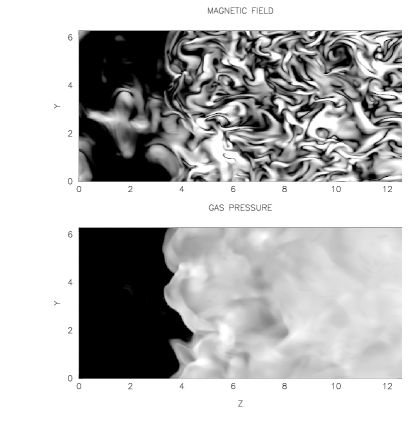
Figure 6: Slices of the magnetic field strength (top) and gas pressure (bottom) through the center of the box obtained at $\tilde{t}=0.12$ in the shock transition region and downstream of the shock. The scaling of the magnetic field strength is logarithmic between $12.6B_{0}$ (black) and $126B_{0}$ (white). The scaling of the gas pressure is also logarithmic between $10^{3}B^{2}_{0}/4\pi$ (black) and $10^{5}B^{2}_{0}/4\pi$ (white). The calculations were performed for a shock propagating with a speed $u_{1}=3000$ km s^-1 in the medium with $V_{a}=10$ km s^-1.

4 MHD modeling in the shock transition region and downstream of the shock

The density fluctuations arising during the development of the non-resonant instability, when the expanding magnetic spirals collide each other (cf. Paper I), play a crucial role in the shock transition region. It is well known, that the propagation of the shock in the medium even with small density fluctuations is accompanied by shock front distortions and the appearance of vortex plasma motions downstream of the shock (see e.g. Kontorovich kontorovich59 (1959), McKenzie & Westphal mckenzie68 (1968), Bykov bykov82 (1982)). These motions can amplify the magnetic field downstream of the shock even in the absence of accelerated particles. This effect was recently observed by Giacalone & Jokipii giacalone07 (2007) in their 2D MHD numerical simulations. The results of low resolution three dimensional calculations for the MHD evolution of an adiabatic supernova remnant in a non-uniform and turbulent interstellar medium were presented by Balsara et al. balsara01 (2001).

Figure 7: Dependence of the physical quantities on $z$ in the shock transition region. Top: random $z$- and perpendicular magnetic field components (normal solid and thin solid lines respectively), $z$- and perpendicular components of the turbulent velocity (thick and thin dashed lines respectively). Bottom: sonic velocity (dotted line), mean gas density (dashed line), mean gas velocity (solid line) in $z$ direction . The calculations were performed for the shock propagating with a speed $u_{1}=3000$ km s^-1 in the medium with $V_{a}=10$ km s^-1.

We investigated this phenomenon and studied the evolution of MHD turbulence in the downstream region. The simulation box with the size $2\pi\times 2\pi\times 4\pi$, stretched in the $z$ direction was used.

The gas flows with the shock velocity $u_{1}$ along the $z$-axis into the box from its left boundary. At the initial moment of time the flat shock front is located at $z=2\pi$. The plasma compression and heating downstream are taken in accordance with the Rankine-Hugoniot conditions. During the simulation the plasma magnetic field, density and pressure are prescribed at the left boundary in accordance with the spatially periodic numerical solution, found in the previous Section. The plasma leaves the system at the right boundary, where the homogeneous boundary conditions are prescribed. The periodic boundary conditions in the perpendicular directions are used. We performed 3D MHD simulation with $256^{2}\times 512$ cells using the numerical method described in Sect.3. The electric current of accelerated particles was switched off.

Figure 8: The one-dimensional spectra of the perpendicular component of the random magnetic field $B_{\perp}(k_{z})$ (solid line), turbulent velocity $U_{\perp}(k_{z})$ (dashed line) and magnetic helicity $H(k_{z})$ (dotted line) downstream of the shock. The calculations were performed for a shock propagating with a speed $u_{1}=3000$ km s^-1 in the medium with $V_{a}=10$ km s^-1. All spectra are normalized to the mean square of the perpendicular component of the random magnetic field.

The obtained numerical results at the shock velocity $u_{1}=3000$ km s^-1 and the Alfvén velocity $V_{A}=10$ km s^-1 are shown in Fig.6 and Fig.7. We used the numerical solution with the normalized shock velocity $u^{\prime}_{1}=4900$ km s^-1 described in the previous Section. The corresponding parameter $\eta_{esc}=0.14$.

The real size of the box in $z$ direction $L_{z}=4\pi/k_{0}$ is related to the distance to the absorbing boundary $L$ as $L_{z}=4\pi LV_{a}/(u_{1}\tilde{t}_{m})$. The value $\tilde{t}_{m}=1.02$ corresponds to the numerical solution with the normalized shock velocity $u^{\prime}_{1}=4900$ km s^-1 described in the previous Section.

The slices of the magnetic field strength and the gas pressure in the $YZ$ plane are shown in the top and bottom panels of Fig.6 respectively. The strong distortions of the shock front and the sonic waves propagating in the downstream region are clearly seen in the bottom panel. The shock front is shifted to the right due to the interaction with the fluid elements which have the enhanced density. The magnetic structures downstream are stretched along the direction of the flow (top panel).

The dependence of the plasma parameters averaged in the perpendicular $XY$ plane on $z$-coordinate is shown in Fig.7. Strong fluctuations of the plasma motions with amplitude of the order of one third of the shock velocity $u_{1}$ exist downstream. It is remarkable that these random motions occur mainly in $z$ direction. The magnetic field is also stretched in this direction. The $z$-component of the random magnetic field is a factor of 1.4 larger than the perpendicular components downstream of the shock.

Figure 9: PDF of the magnetic field $P_{B}(B)$ (thin solid line), turbulent velocity $P_{U}(u)$ (thin dashed line) and density $P_{\rho}(\rho)$ (thin dotted line) downstream of the shock. The analytical approximation for PDF of the magnetic field (23) (thick dotted line) is also shown. The calculations were performed for a shock propagating with a speed $u_{1}=3000$ km s^-1 in the medium with $V_{a}=10$ km s^-1.

The spectra of the magnetic field, the plasma velocity and the magnetic helicity downstream of the shock are shown in Fig.8. Note, that the magnetic helicity is not zero in this region.

PDF distributions of the random magnetic field, turbulent velocity and plasma density obtained downstream of the shock are shown in Fig.9.

The numerically calculated magnetic compression ratio $\sigma_{B}$ is about 3.0 in this simulation with the shock compression ratio $\sigma$ close to 4. This value of $\sigma_{B}$ is close to one that is expected if the isotropic random magnetic field is compressed at the shock front: $\sigma_{B}=\sqrt{(2\sigma^{2}+1)/3}$. Since in the real situation the pressure of accelerated cosmic ray particles should be taken into account, the shock compression will be higher. We found that the use of the adiabatic index $\gamma=4/3$ with the corresponding shock compression ratio about 6 results in a magnetic compression factor $\sigma_{B}$ close to 3.5, that is smaller than the expected value $\sigma_{B}\sim 5$. Probably this is due to the numerical dissipation of the field. It is necessary to have a better numerical resolution in the last case since the stronger compression of the field at the shock front results in the stronger numerical dissipation. We obtained the close value of $\sigma_{B}=2.6$ in the simulation with $\gamma=5/3$ and the lower numerical resolution $256\times 128^{2}$. This demonstrates that the resolution $512\times 256^{2}$ is good enough for the simulation of the shock with the compression ratio 4. We found that the corresponding values of $\sigma_{B}$ differ significantly from each other in the case of the higher shock compression ratio.

5 Analytical estimate of the maximum energy of accelerated particles in SNR

Now we can estimate analytically the maximum particle energy achieved in the process of acceleration. We shall use Eq. (5) and assume that the random field is isotropic and concentrated at the wavenumber $k$, so that $b=B_{r}^{2}/(2k)$ where the rms of the random magnetic field $B_{r}=\left<\delta B^{2}\right>^{1/2}$. Let us change the integration on $dz$ to the integration on time $dt=dz/u_{1}$ in Eq. (5). The evolution of the amplified magnetic field can be approximately described as

$$B_{r}(t)=\left\{\begin{array}[]{ll}B_{b}\exp(\gamma_{\max}t),\ t<t_{1}=\gamma_{\max}^{-1}\ln\frac{2B_{0}}{B_{b}}\\ 2B_{0}(1+\gamma_{\max}(t-t_{1})),\ t>t_{1}\end{array}\right.$$ (15)

Here $B_{b}$ is the initial value of the amplified field. At the first stage $t<t_{1}$ the field is amplified exponentially in time with the maximum growth rate $\gamma_{\max}=j_{d}B_{0}/2c\rho_{0}V_{a}$ (cf. Paper I). The corresponding wavenumber $k$ is $k=2\pi j_{d}/cB_{0}$ at this stage. At the second stage $t>t_{1}$ the field is amplified linearly in time. The wavenumber $k$ may be found from the expression $kB_{r}=4\pi j_{d}/c$. This dependence of random magnetic field on time is in a qualitative agreement with the simulations of the non-resonant instability (cf. Paper I).

The integration of Eq. (5) gives

$$p_{m}^{2}=\frac{3\pi}{4}\frac{q^{2}u_{1}^{2}B_{0}^{2}V_{a}}{\gamma_{\max}^{2}c^{3}}\left\{\begin{array}[]{ll}B_{r}^{2}/(2B_{0}^{2}),\ t_{m}<t_{1}\\ 1+(1+\gamma_{\max}(t_{m}-t_{1}))^{4},\\ t_{m}>t_{1}.\end{array}\right.$$ (16)

Here $t_{m}=L/u_{1}$. The electric current $j_{d}$ that drives the instability is constant over the whole region $-L<z<0$ except the narrow zone near the shock (see Fig.3). The input of this zone was neglected in Eq. (16). This assumption introduces a relatively small error into the calculation of $p_{m}$, since Eq. (16) is an implicit equation for $p_{m}$. The growth rate $\gamma_{\max}$ is inversely proportional to $p_{m}$ (see Eq. (17) below). Thus $p_{m}$ remains in Eq. (16) only through $\gamma_{\max}$ after the parenthesis. This produces an error in the evaluation of $t_{m}$ and $p_{m}$ that is not larger than 10 percent.

Using Eq. (9) we estimate $j_{d}=\eta_{esc}q\rho u_{1}^{3}/(2cp_{m})$ and

$$\gamma_{\max}=\frac{\eta_{esc}}{4}\frac{qu_{1}^{3}B_{0}}{V_{a}c^{2}p_{m}}.$$ (17)

From these two equations we finally obtain the value of the amplified field

$$B_{r}=2B_{0}\left\{\begin{array}[]{ll}u_{1}^{2}/u_{*}^{2},\ u_{1}<u_{*}\\ \left(2\frac{u_{1}^{4}}{u_{*}^{4}}-1\right)^{1/4},\ u_{1}>u_{*}\end{array}\right.$$ (18)

and the maximum energy of accelerated particles

$$p_{m}c=\frac{\eta_{esc}qu_{1}^{2}B_{0}L}{4cV_{a}}\left\{\begin{array}[]{ll}\ln^{-1}\left(\frac{2B_{0}u_{1}^{2}}{B_{b}u_{*}^{2}}\right),u_{1}<u_{*}\\ \left[\ln\left(\frac{2B_{0}}{B_{b}}\right)-1+\left(2\frac{u_{1}^{4}}{u_{*}^{4}}-1\right)^{1/4}\right]^{-1},\\ u_{1}>u_{*}\end{array}\right.$$ (19)

where the velocity $u_{*}=(24\pi cV_{a}^{3}/\eta_{esc}^{2})^{1/4}$.

Using the first line of expression (19) for an arbitrary shock velocity $u_{1}$ we obtain the upper limit of the maximum energy. The growth rate (17) calculated with this maximum energy is high enough to provide the considerable magnetic field growth during the age of a supernova remnant (to be compared with Bell bell04 (2004)). The upper limit and the maximum energy (19) for $\ln\left(2B_{0}/B_{b}\right)=5$ are shown in Fig.2. We found that for $u_{1}>>u_{*}$ Eq. (18) gives the amplified field a factor of 2 smaller than the numerical results (see Table 1). It is because we neglected the growth of the diffusive current $j_{d}$ in the narrow zone just adjacent to the shock in our analytical estimates. However, this does not influence the estimate of the maximum energy (19).

Table 2: Maximum energies and amplified magnetic fields in historical SNRs.

	$T\tablenotemark{a}$	$u_{1}\tablenotemark{b}$	$n_{H}\tablenotemark{c}$	$B_{0}\tablenotemark{d}$	$u_{1}^{\prime}\tablenotemark{e}$	$u_{1}^{\prime}\tablenotemark{e}$	$u_{1}^{\prime}\tablenotemark{e}$	$p_{m}c\tablenotemark{f}$	$p_{m}c\tablenotemark{f}$	$p_{m}c\tablenotemark{f}$	$B_{d}\tablenotemark{g}$	$B_{d}\tablenotemark{g}$	$B_{d}\tablenotemark{g}$	$B_{d}^{obs}\tablenotemark{h}$
$\eta_{esc}$					0.01	$0.05$	$0.14$	0.01	$0.05$	$0.14$	0.01	$0.05$	$0.14$
Tycho	435	4500	0.3	5.0	1360	3040	5090	19	76	170	21	110	260	300
SN1006	1000	4300	0.1	5.0	860	1920	3220	22	100	240	8.4	43	120	140
Kepler	400	5300	0.35	5.0	1670	3800	6360	30	115	250	33	160	350	215
Cas A	330	5200	3.0	10.0	2220	4960	8300	63	230	500	120	510	980	485

For the fast shocks $u_{1}>>u_{*}$ the amplified upstream magnetic field may be estimated using the formula

$$\frac{B^{2}}{4\pi}\sim 2\eta_{esc}\rho u_{1}^{2}\sqrt{\frac{V_{a}}{c}}.$$ (20)

For velocities $u_{1}>u_{*}$ Eq. (19) may be rewritten as

$$\frac{p_{m}c}{Z}=21\ \mathrm{TeV}\ \frac{\frac{\eta_{esc}}{0.05}\left(\frac{u_{1}}{1000\ \mbox{km s}^{-1}}\right)^{2}n_{H}^{1/2}L_{pc}}{\ln\left(\frac{2B_{0}}{B_{b}}\right)-1+\left(2\frac{u_{1}^{\prime 4}}{u_{3}^{4}}-1\right)^{1/4}},$$ (21)

where $Z$ is the charge number of accelerated particles, $u_{3}=1730$ km s^-1, $n_{H}$ is the hydrogen number density in cm^-3 and $L_{pc}$ is the size $L$ in parsecs. Note that the denominator of this equation contains the normalized shock velocity (12).

For three-dimensional shocks this equation may be considered as a rough estimate of the maximum energy of accelerated particles. Then the size $L$ is related to the shock radius $R$ and the remnant age $T$ as $L=m_{0}R=u_{1}T$.

6 Discussion

The initiation of the MHD streaming instability by accelerated particles in the shock precursor is an integral part of the efficient diffusive shock acceleration process. The instability is non-resonant if the electric current of accelerated particles is large enough, so that the normalized shock velocity exceeds some critical value

$$u_{1}>(4cV_{a}^{2}/\eta_{esc})^{1/3}$$

$$=1340\ \mbox{km s}^{-1}\left(\frac{V_{a}}{\mbox{10 km s}^{-1}}\right)^{2/3}\left(\frac{\eta_{esc}}{0.05}\right)^{-1/3}.$$ (22)

This equation is equivalent to Eq. (18) in Paper I.

The non-resonant character of this instability means that the principal scale of the growing random magnetic field remains smaller than the gyroradius of particles with momentum close to its maximum value $p_{m}(t)$. The treatment of the non-magnetized particle scattering is relatively simple and it allowed us to fulfill the numerical simulation of the diffusive shock acceleration accompanied by the strong streaming instability and to make the corresponding analytical estimates. The calculated amplification of magnetic field in young SNR proved to be very significant. The maximum energy of accelerated particles is mainly limited by the finite time of the growth of magnetic disturbances. The analytical estimate of the maximum particle momentum is given by Eq. (19) and it is in agreement with our numerical results presented in Fig.2. The resulting maximum momentum is not as high as one may expect using the Bohm diffusion coefficient in the amplified field since the scattering by the small scale field is not so efficient.

The small-scale field approximation is broken for particles with relatively low energies when their gyroradii in the amplified magnetic field are smaller than the principal scale of the field. Roughly it occurs when the scattering frequency of the particle is smaller than its gyrofrequency in the amplified field. The ratio of these quantities for particles with the maximum momentum $p_{m}$ is the ratio of the numbers from the 7th and 3rd lines of Table 1. This ratio is close to 1 for the smallest considered normalized velocity $u_{1}^{\prime}=1550$ km s^-1 when the small-scale approximation is only marginally valid. The ratio decreases if the shock velocity increases. This ratio is close to 1/3 for the normalized velocity $4900$ km s^-1 that is the representative value for the young historical supernovae (see below) . This means that for this shock velocity the small-scale approximation is valid for particles with the normalized momentum larger than $p_{m}^{\prime}/3$. For particles with smaller energies the amplified magnetic field can be considered as the mean large-scale field. These particles are resonantly scattered by the magnetic inhomogeneities from the inertial range of the magnetic spectrum (see Fig.4) or by the magnetic perturbations produced by the resonant streaming instability of these particles (cf. Pelletier et al. pelletier06 (2006)).

It is interesting that formula (21) without the root in the denominator may be used to estimate the maximum energy of particles, accelerated at slow astrophysical shocks when the condition (22) is violated and the resonant streaming instability should be taken into account. The matter is that the expression for the increment of the non-resonant instability (17) differs from the increment of the resonant instability only by a factor of the order of unity (see e.g. Berezinskii et al. berezinsky90 (1990)). This is why the expression (21) may be also used for slow shocks provided that the wave damping does not quench the development of instability that is relatively slow in this case. It may be in a highly ionized medium where the damping of MHD waves on neutrals is negligible. Nonlinear damping of Alfvén waves may be also depressed in a plasma with $\beta>0.3$, since the presence of waves, propagating in the opposite to the cosmic ray streaming direction is necessary for this damping (Zirakashvili zirakashvili00 (2000)). Such waves may appear only in a collisionless low-$\beta$ plasma due to the nonlinear induced scattering (Livshits & Tsytovich livshits70 (1970)), or due to the three-wave interactions in the framework of magnetohydrodynamics (Chin & Wentzel chin72 (1972)).

Because the particles at the end of the spectrum are scattered by the small-scale magnetic field, the spectrum has the universal shape in the cut-off region described by Eqs (7) and (8) in the case of high velocity shocks. This is important for the calculation of gamma-ray production by the nucleon component in SNRs.

The comparison of the predicted values of amplified fields given in Table 1 with the values derived from the thickness of X-ray filaments of young SNRs (see e.g. Völk et al. voelk05 (2005)) shows reasonable agreement, if the acceleration efficiency is not low: $\eta_{esc}>0.05$.

The calculated downstream magnetic fields and the maximum energies obtained for the historical SNRs with known ages are given in Table 2. We use the same supernova parameters as Vink vink06 (2006). We assumed the standard interstellar value of the magnetic field $B_{0}=5\ \mu$G for SNRs Kepler, Tycho and SN1006. The accepted magnetic field strength $B_{0}=10\ \mu$G for Cas A supernova gives the value of the Alfvén velocity about 10 km s^-1 that is a reasonable number for the stellar wind produced at the Red Supergiant stage of the likely progenitor of this supernova. The magnetic field amplified upstream of the shock is determined by the value of the normalized shock velocity $u_{1}^{\prime}$ and is given in the 3rd line of Table 1. This almost isotropic random magnetic field is further amplified by a magnetic compression factor $\sigma_{B}=4$ in the shock transition region.

One of the key parameters in our calculations $\eta_{esc}$ is in principle determined by the injection efficiency of thermal particles in the process of acceleration and by the degree of shock modification by the cosmic ray pressure, see Berezhko and Ellison berezhko99 (1999) and Blasi et al. blasi05 (2005). The value of $\eta_{esc}$ can not be calculated theoretically yet and we used different $\eta_{esc}$ in our estimates. The results obtained for three values $\eta_{esc}=0.01$, $\eta_{esc}=0.05$ and $\eta_{esc}=0.14$ are shown in Table 2. The value $\eta_{esc}=0.14$ is realized for the plain cosmic ray modified shock with the compression ratio $\sigma=6$ and the thermal sub-shock compression ratio $\sigma_{s}=2.5$. The second value $\eta_{esc}=0.05$ corresponds to the situation when due to some reason the shock modification is weaker. The value $\eta_{esc}=0.01$ corresponds to the non-modified shock with the cosmic ray pressure $P_{\mathrm{CR}}$ about ten percents of the ram pressure $\rho_{0}u_{1}^{2}$.

The maximum energies of particles accelerated in Kepler, Tycho and SN1006 supernovae that all are of the Ia type are about $100\div 300$ $Z$ TeV. These maximum energies were not strongly different in the past during the free expansion stage of the remnant evolution since the higher shock velocity was almost compensated by the smaller shock radius in Eq. (21).

The similar maximum energies are predicted for the core collapse IIP supernovae. They have large ejected masses about $M_{ej}\sim 10M_{\odot}$ and correspondingly relatively low expansion velocities of the order of $3000$ km s^-1 (see Chevalier chevalier05 (2005) for a review).

The situation is different and the maximum particle energies can be higher in the case of the core collapse Ib/c and IIb supernovae. These supernovae have high initial velocities about $3\cdot 10^{4}$ km s^-1, small ejected masses $M_{ej}=1\div 3\ M_{\odot}$ and the circumstellar medium corresponding to the dense red supergiant stellar wind (IIb supernovae ) or the interaction zone between the fast stellar wind of a Wolf-Rayet progenitor and the slow red supergiant wind (Ib/c supernovae) with strong magnetic fields (see Chevalier chevalier05 (2005) for a review). In the present paper we have considered the acceleration of particles and the generation of the MHD turbulence at the parallel shock and our theory can not be directly applied to this type of supernovae because the magnetic field in the stellar wind is azimuthal. However, it is possible that stellar winds contain significant random magnetic fluctuations and we may expect that some part of a SNR shock surface may be treated as a parallel shock. This also will provide the injection of thermal particles into the diffusive shock acceleration process since it is known that the injection of thermal ions occurs preferentially at the parallel shocks (see Völk et al. voelk03 (2003) for discussion of these topics).

The Cas A is a Ib type supernova. The maximum energy was larger in the past because the small radius of the shock in Eq. (21) was compensated by the higher gas density of the stellar wind and the higher shock velocity. Thus the velocity $u_{1}=10^{4}$ km s^-1 gives the maximum energy $p_{m}c=1.2$ $Z$ PeV. Therefore such supernovae can accelerate cosmic ray protons up to PeV energies.

Because the maximum momentum (21) decreases at the Sedov stage when the age of the remnant increases, the highest energy particles leave the remnant. The overall spectrum produced by the SNR is formed in this manner (Ptuskin & Zirakashvili ptuskin05 (2005)) with the energy spectrum close to $E^{-2}$. At the earlier free expansion stage when only a small amount of the supernova ejecta energy is transferred to the supernova shock the steep high energy tail in the spectrum is formed ( Berezhko & Völk berezhko04 (2004), Ptuskin & Zirakashvili ptuskin05 (2005)). This means that the particles from the end of the cosmic ray spectrum produced by the given supernovae are accelerated at the end of the free expansion stage when the shock velocity is of the order of the characteristic ejecta velocity. It is about $7000\div 10000$ km s^-1 for Ia/b/c and IIb supernovae.

We should note that the shock velocities in Table 2 are based on radio and X-ray expansion measurements. If we use the lower shock velocities from Völk et al. voelk05 (2005), the corresponding maximum energies are a factor of 2 smaller.

It is clear from Fig.7 that the amplified magnetic field does not drop downstream of the shock. Its level is maintained by the turbulent motions produced by the interaction of density inhomogeneities with the shock front. However, the amplitude of these motions slowly decreases downstream of the shock. At some distance magnetic and kinetic energies will become equal to each other. At larger distances magnetic dissipation may occur. These distances are larger than $2\div 3L_{z}$ according to Fig.7. We conclude that the dissipation length of the magnetic field downstream of the shock is not smaller than $0.1L$ in our numerical simulation.

The interaction of the shock front with density disturbances results in the shock front deformation (see Fig.6). The thickness of X-ray rims produced by the synchrotron cooling of accelerated electrons should increase correspondingly up to the values about 0.01$L$ according to Fig.7 (a so-called projection effect is not taken into account here). Probably this is the reason for the relatively small value of the magnetic field $485$ $\mu$G in Cas A inferred from the width of X-ray filaments in comparison with the theoretical value expected at $\eta_{esc}>0.05$, see Table 2.

The characteristic time of the random motions of the shock front is given by the ratio of the size of density inhomogeneities and the shock velocity. It is about one year for the size of density inhomogeneities $10^{16}$ cm in young historical SNRs. The value $L=0.5R=1.5$ pc was assumed for this estimate.

PDF of the magnetic field downstream of the shock that is shown in Fig.9 is described with a good accuracy by the following function:

$$P_{B}(B)=\frac{\sqrt{6}B}{\left<B^{2}\right>}\exp{\left(-\sqrt{6}B/\left<B^{2}\right>^{1/2}\right)}.$$ (23)

The exponential tails of the magnetic PDF appear to be a fairly universal feature of turbulently amplified magnetic fields (Brandenburg et al. brandenburg96 (1996), Schekochihin et al. schekochihin04 (2004)).

As one can see from Table 1, the electric potential $\phi$ has rather large values for the fast shocks with velocities $u_{1}^{\prime}>30000$ km s^-1. The mean electric field is directed opposite to the direction of the diffusive electric current. This electric field drags the particles which produce the instability toward the shock. It may create the steepening of the spectrum of these particles. If there is a small amount of oppositely charged particles (electrons), their spectrum should be somewhat flatter.

7 Conclusion

We have investigated the acceleration of particles at the fast plane parallel shock. The generation of MHD turbulence by the non-resonant streaming instability (Bell bell04 (2004)) was taken into account. We solved this problem using only first principles and with a minimum of simplifying assumptions. We combined the analytical solution for the particle acceleration and the numerical MHD calculations for the evolution of the MHD turbulence. The following results were obtained:

1) For the relatively fast shocks when the condition (22) is satisfied, the particles at the high-energy end of the spectrum are scattered by small-scale random magnetic fields generated by the non-resonant streaming instability. Their spectrum has the universal shape given by Eq. (8).

2) The MHD turbulence is mainly generated by the streaming of run-away particles at large distance from the shock. The level of the MHD turbulence is the highest in the shock vicinity. The accelerated particles are concentrated in the same region. This means that the acceleration of particles can be considered in the one-dimensional approximation even for a three-dimensional system. The characteristic width of the particle distribution in our simulations is not larger than $0.1\ L$ (see Fig.3 and 10th line of Table 1).

3) It is important, that the non-resonant instability produces strong density fluctuations upstream of the shock (see Sect.4 and Paper I). These fluctuations produce a strong deformation of the shock front and fast vortex motions downstream of the shock. That is why the magnetic amplification in the shock transition region is not reduced to a simple compression of the magnetic field in the direction perpendicular to the shock front. The magnetic field is also stretched by the flow motions in the direction perpendicular to the shock front. As a result, the magnetic field component which is perpendicular to the shock front is a factor of 1.4 larger than the parallel components downstream of the shock. This naturally explains the preferable radial orientation of magnetic fields in young SNRs.

The characteristic time 1 year of the shock deformation and of the corresponding MHD fluctuations found here (see Sect.6) is of particular interest in the light of the last results on variability of X-ray emission observed in RXJ1713 SNR (Uchiyama et al. uchiyama07 (2007)).

4) The dissipation of the magnetic field downstream of the shock is relatively slow in our simulation. If so, the origin of X-ray filaments, observed in young SNRs, is related to the fast synchrotron cooling of accelerated electrons but not to the decay of the MHD turbulence.

5) The values of the calculated amplified magnetic field are similar to those, observed in historical SNRs, if the energy flux of the run-away particles is not low: $\eta_{esc}>0.05$ (see Table 2).

6) The magnetic field growth is only linear in time for the fast shocks with the normalized velocities higher than about ten thousand km s^-1. This reduces the maximum energy of accelerated particles compared to the case of the exponential growth. For these shocks the energy of the magnetic field amplified upstream is a small fraction $\sqrt{V_{a}/c}$ of the energy density of the highest energy particles (see Eq.(20)). The magnetic field amplification is relatively weak for slow shocks with the normalized velocities 1230 km s^-1 and smaller (see Eq.(18)).

7) We calculated numerically the maximum energy of accelerated particles (see Fig.2). This energy may be described by the analytical formula (19). The maximum energies of particles are higher than the energies obtained in the Bohm limit in the background magnetic field (see the 7th line of the Table 1) but lower than the energies obtained using the Bohm limit in the amplified field. The significantly long time of the random magnetic field growth is the main factor that limits the maximum energy of accelerated particles. We calculated the maximum energies for four historical SNRs (Table 2).

8) Using the last result we found that the maximum energy of cosmic ray protons accelerated by Ia and IIP supernovae is about $100\div 300$ TeV. Only Ib/c and presumably IIb supernovae may accelerate protons up to PeV energies. Since it is expected that the explosion rate is the highest for IIP supernovae, we should observe a change of the slope of the galactic cosmic ray spectrum at the energies of the order of 100 TeV.

9) The MHD turbulence generated by the non-resonant streaming instability has a non-zero magnetic helicity. The helical Lorentz force produces corresponding plasma motions and the mean electric field ${\bf E}_{0}$ that is in the opposite direction to the electric current of energetic particles. This electric field modifies the cosmic ray transport equation (see Paper I). This effect is significant for very fast shocks with velocities larger than 30 thousands km s^-1. The presence of this field should result in the steepening of the spectrum of particles which produce the non-resonant instability (presumably nucleons) and the flattening of the spectrum of oppositely charged particles (presumably electrons).

Appendix A The dependence of scattering on pitch angle.

If the random field is not isotropic the same is true for the particle scattering. Let us assume that the random magnetic field is isotropic in the plane perpendicular to the mean magnetic field ${\bf B}_{0}$ and that the cosmic ray distribution $f_{0}$ depends only on pitch angle $\theta$. Now the scattering operator described by the tensor $\nu_{ij}$ (cf. Paper I) can be written as

$$\frac{\partial}{\partial p_{i}}\nu_{ij}\frac{\partial f_{0}}{\partial p_{j}}=\frac{\partial}{\partial\mu}\frac{\nu_{0}(\mu)}{2}(1-\mu^{2})\frac{\partial f_{0}}{\partial\mu},$$ (A1)

where $\mu=\cos{\theta}$. The scattering frequency $\nu_{0}(\mu)$ can be expressed in terms of the spectrum of $y$-component of the random magnetic field (mean field is in $z$ direction):

$$\nu_{0}(\mu)=2\pi\frac{q^{2}v}{p^{2}c^{2}}\int d^{3}kB_{yy}({\bf k})\delta(k_{z}\mu+k_{x}\sin{\theta}).$$ (A2)

The parallel diffusion coefficient $D_{\parallel}$ can be written now as (see e.g. Berezinskii et al. berezinsky90 (1990))

$$D_{\parallel}=\frac{v^{2}}{2}\int\limits^{1}_{0}d\mu\frac{1-\mu^{2}}{\nu_{0}(\mu)}.$$ (A3)

References

- (1) Achterberg, A., 1983, A&A, 119, 274
- (2) Axford, W.I., Leer, E., Scadron, G., 1977, Proc. 15th Int. Cosmic Ray Conf., Plovdiv, 90, 937
- (3) Balsara, D., Benjiamin, R.A., & Cox, D.P., 2001, ApJ, 563, 800
- (4) Bamba, A., Yamazaki, R., Ueno, M., & Koyama, K., 2003, ApJ, 589, 827
- (5) Bamba, A., Yamazaki, R., & Hiraga, J.S., 2005, ApJ, 632, 294
- (6) Bell, A.R., 1978, MNRAS, 182, 147
- (7) Bell, A.R., 2004, MNRAS, 353, 550
- (8) Berezhko, E.G., Ksenofontov L.G., & Völk, H.J. 2002, A&A 395, 943
- (9) Berezhko, E.G., & Völk, H.J. 2004, A&A 427, 525
- (10) Berezhko, E.G., & Ellison, D.C., 1999, ApJ 526, 385
- (11) Berezinskii V.S., Bulanov, S.V., Dogiel, V.A., Ginzburg, V.L., & Ptuskin, V.S., 1990, Astrophysics of Cosmic Rays, North Holland, NY
- (12) Brandenburg, A., Jennings, R.L., Nordlund, A., Rieutord, M., Stein, R.F., & Tuominen, 1996, J.Fluid Mech., 306, 325
- (13) Blasi, P., Gabici, S., & Vannonoi, G., 2005, MNRAS, 361, 907
- (14) Blandford, R.D., & Ostriker, J.P. 1978, ApJ, 221, L29
- (15) Bykov A.M., 1982, Soviet Astron. Letters, 8,596
- (16) Chevalier, R., 2005, ApJ, 619, 839
- (17) Chin, Y, & Wentzel, D.G., 1972, Astrophys. and Space Sci. 16, 465
- (18) Giacalone, J., & Jokipii, J.R., 2007, ApJ 663, L41
- (19) Dolginov, A.Z., & Toptygin, I.N. 1967, JETP, 24, 1195
- (20) Gotthelf, E.V., Halpem, J.P., Camilo, F. et al. 2001, ApJ, 552,L125
- (21) Gull, S.F., 1975, MNRAS, 171, 263
- (22) Hwang, U., Decourchelle, A., Holt, S.S., & Petre, R., 2002, ApJ, 581, L101
- (23) Kontorovich V.M., 1959, Acoustic Journal 5, 314 (in Russian)
- (24) Krymsky, G.F. 1977, Soviet Physics-Doklady, 22, 327
- (25) Livshits, L.M., & Tsytovich, V.N., 1970, Nuclear Fusion 10, 240
- (26) Long, K.S., Reynolds, S.P., Raymond, J.C., Winkler, P.F., Dyer, K.K., & Petre, R., 2003, ApJ, 586, 1162
- (27) Malkov, M.A., & Drury, L.O’C, 2001, Reports on Progress in Physics, 64, 429
- (28) McKenzie, J.F., & Westphal, K.O., 1968, Phys. Fluids, 11, 2350
- (29) McKenzie, J.F., & Völk, H.J., 1982, A&A, 116, 191
- (30) Milne, D.K., 1987, Australian J.Phys., 40, 771
- (31) Pelletier, G., Lemoine, M., & Marcowith, A., 2006, A&A, 453, 181
- (32) Pohl, M., Yan, H., & Lazarian, A., 2005, ApJ, 626, L101
- (33) Ptuskin, V.S., & Zirakashvili, V.N. 2005, A&A, 429, 755
- (34) Schekochihin, A.A., Cowley, S.C., & Taylor, S.F., 2004, ApJ, 612, 276
- (35) Uchiyama, Y., Aharonian, F.A., Tanaka, T., Takahashi, T., & Maeda, Y., 2007, Nature, 499, 576
- (36) Vink, J., & Laming, J.M., 2003, ApJ, 584, 758
- (37) Vink, J., 2006, Proceedings of the Symposium ’The X-ray Universe 2005’, San Lorenzo de El Escorial, Spain, 26-30 September 2005, astro-ph/0601131
- (38) Völk, H.J., Berezhko, E.G., & Ksenofontov, L.T., 2003, A&A 409, 563
- (39) Völk, H.J., Berezhko, E.G., & Ksenofontov, L.T., 2005, A&A 433, 229
- (40) Zirakashvili, V.N. 2000, JETP 90, 810
- (41) Zirakashvili, V.N., Ptuskin, V.S., & Völk, H.J., 2008, ApJ submitted (Paper I)