Limits on the Position Wander of Sgr A*

Abstract

We present measurements with the VLBA of the variability in the centroid position of Sgr A* relative to a background quasar at $7\,{\rm m}{\rm m}$ wavelength. We find an average centroid wander of $71\pm 45\,\mu{\rm as}$ for time scales between 50 and $100\,\min$ and $113\pm 50\,\mu{\rm as}$ for timescales between 100 and $200\,\min$, with no secular trend. These are sufficient to begin constraining the viability of the accretion hot-spot model for the radio variability of Sgr A*. It is possible to rule out hot spots with orbital radii above $15\,GM_{\rm SgrA*}/c^{2}$ that contribute more than 30% of the total $7\,{\rm m}{\rm m}$ flux. However, closer or less luminous hot spots remain unconstrained. Since the fractional variability of Sgr A* during our observations was $\sim 20$% on time scales of hours, the hot-spot model for Sgr A*’s radio variability remains consistent with these limits. Improved monitoring of Sgr A*’s centroid position has the potential to place significant constraints upon the existence and morphology of inhomogeneities in a supermassive black hole accretion flow.

1 Introduction

There is now overwhelming evidence that Sgr A* is a supermassive black hole at the center of the Milky Way. Many stars are observed to orbit about a common focal position, requiring an unseen mass of $\approx 4\times 10^{6}$ M_⊙ contained within a radius of less than 100 AU (Schödel et al. 2002; Ghez et al. 2003), for a distance to the center of 8.0 kpc (Reid 1993). Accurate registration of the infrared and radio reference frames (Menten et al. 1997; Reid et al. 2003) reveal that the common orbital focal position is coincident with Sgr A* to within measurement uncertainty of $\approx 10$ mas. Finally, the absence of intrinsic motion of Sgr A* at levels near that expected for a $4\times 10^{6}$ M_⊙ object (Reid & Brunthaler 2004), coupled with a size less than  1 AU (see, e.g., Bower et al. 2004), provide a lower limit on mass density of $\sim 10^{22}$ M_⊙ pc^-3, which is only two orders of magnitude less than the density of a $4\times 10^{6}$ M_⊙ non-rotating black hole within its innermost stable orbit. There can now be little doubt that Sgr A* is a supermassive black hole.

Reid & Brunthaler (2004) present measurements of the position of Sgr A* relative to a compact extragalactic radio source (J1745$-$2820, also refered to as J1745-283 in earlier publications). These measurements were conducted with the NRAO Very Long Baseline Array (VLBA) over a period of $8\,{\rm yr}$ at a wavelength of $7\,{\rm m}{\rm m}$ ($43\,{\rm GHz}$) and have been used to determine the apparent proper motion of Sgr A*. Over time scales of months or longer, Sgr A*’s apparent motion is dominated by the effects of the orbit of the Sun about the center of the Galaxy. The component of the Sun’s orbit in the Galactic plane is uncertain at roughly the 10% level, and this limits estimation of any intrinsic motion of Sgr A* at about the $\pm 20$ km s^-1 level. However, the component of the motion of the Sun out of the Galactic plane is known to high accuracy [$7.16\pm 0.38$ km s^-1 toward the North Galactic Pole; Dehnen & Binney (1998)]. After removing the effects of the Sun’s motion, the residual motion of Sgr A* perpendicular to the Galactic plane is very small, $\lesssim 1\,{\rm k}{\rm m}\,{\rm s}^{-1}$, as expected for a supermassive black hole (SMBH) at the dynamical center of the Galaxy. While previous work concentrated on the long-term motion of Sgr A*, here we analyze its short-term position “wander” on time scales of hours to weeks.

Short-timescale motion of the centroid position of Sgr A* would be expected if a portion of the emission comes from material orbiting about the SMBH. The degree of centroid variability would necessarily depend upon the brightness of the orbiting material, the degree to which its emission is nonuniform, and the orbital radius dominating the total flux. We use a simple hot-spot model to relate the constraint from the observed short-term position wander of Sgr A* (§2) to a constraint upon the presence of strong inhomogeneities in the accretion flow onto the SMBH as a function of hot-spot luminosity and orbital period (§3). Finally, concluding remarks are contained in §4.

2 Observations of Centroid Motion

Reid & Brunthaler (2004) describe the observations and data calibration methods in detail. Briefly, we obtained position data as follows: the VLBA antennas switched between Sgr A* and a compact extragalactic source (J1745$-$2820) every 15 seconds in order provide interferometer phase differences rapidly enough to cancel the effects of short term atmospheric fluctuations. The stronger source, Sgr A*, was used as the phase reference to calibrate data from the weaker source, J1745$-$2820.

Astrometric imaging of Sgr A* at 7-mm wavelength is best accomplished with only the five inner-VLBA antennas (FD, KP, LA, OV and PT). These antennas produce interferometer baselines with lengths of up to $1500$ km, resulting in synthesized beams typically about $2.5\times 0.7$ mas (FWHM) elongated north-south. Longer baselines (e.g. involving the Washington (BR) and Iowa (NL) state antennas) are not generally useful for precise astrometry, as it is difficult to detect Sgr A* with the 8-sec on-source integrations afforded by rapid switching, coupled with low fringe visibilities on long baselines owing to the large, scatter-broadened, image of Sgr A*. Also, the sources are mutually visible with the inner five antennas for only a short time period for antennas far from the inner ones.

Our most accurate astrometry was obtained with atmospheric path-delay calibration using “geodetic” blocks (Reid & Brunthaler 2004). This involves short periods of observations of quasars with a wide spanned-bandwidth and scheduled to deliver a wide range of source elevations. These geodetic blocks were placed before the start, at the middle, and after the end of the Sgr A* observations. Analysis of these data yield estimates of the zenith atmospheric path-delay at each antenna accurate to $\sim 0.5$ to 1 cm (or about 1 wavelength).

2.1 Position wander: hours

For analysis of short-term wander, we selected only our highest quality data, requiring both high accuracy atmospheric path-delay calibration using geodetic blocks (which was started in 2003) and data from all five inner-VLBA antennas. Data from VLBA programs BR84 on 2003 April 5 and 25 and BR124 on 2007 April 5 and 11 satisfied these requirements.

The position wander of Sgr A* over time scales of hours was determined by dividing the calibrated interferometer data into hourly bins. The data were Fourier transformed to make images and intensity centroid positions were determined. In practice, we measured the background source, J1745$-$2820, which had been phase-referenced to Sgr A*, but we interpret any position changes as owing to changes in Sgr A*. In Fig. 1 we show the East-West (EW) position offsets as a function of Greenwich sidereal time, after removing an average position for each day’s data. The North-South (NS) positions are intrinsically less accurate by a factor of about 3, as the NS projections of the interferometer baselines are correspondingly shorter than the EW projections.

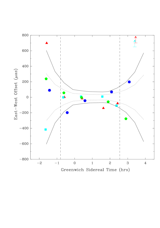
Figure 1: Hourly measurements of the centroid position of Sgr A* relative to an extragalactic source. Data from 2003 April 05 (red triangles) and 25 (cyan squares) and 2007 April 05 (green pentagons) and 11 (blue hexagons) are plotted. All positions are relative to their daily average position. Dotted and solid lines indicate expected $\approx 1\sigma$ and $\approx 2\sigma$ uncertainties, based on Monte Carlo simulations of the effects of uncompensated atmospheric path-delays (0.5 cm rms) at each antenna. Data outside the vertical dashed lines were excluded from analysis owing to their large expected position errors.

At the start and end of the observing tracks, the sources are at low elevations and susceptible to large interferometer phase shifts caused by uncompensated atmospheric path-delays. We estimated the effects of zenith path-delay errors with 1000 independent simulations. Each simulation started by randomly selecting zenith path-delay errors (0.5 cm rms) for each antenna. We then calculated the expected interferometer phase shifts, dependent on time-varying source zenith angles, at half-hour time steps. Position shifts were estimated as the product of the phase shifts (in turns) multiplied by an approximate projected interferometer fringe spacing. Finally, we calculated a weighted position shift for all baselines and all times when the source was above $15^{\circ}$ elevation. The resulting expected $\pm 1\sigma$ and $\pm 2\sigma$ position error envelopes are plotted in Fig. 1. Based on the observed and simulated increase in position scatter for Greenwich sidereal times (GST) before $-0.8$ hr and after $+2.6$ hr, we only use data within this time range for our study of hourly position wander.

We differenced the EW and NS positions for all pairs of measurements separated by less than $10^{3}$ min; the magnitudes of these position differences are shown on the left-hand side of Fig. 2, along with 2 binned weighted averages. The average difference in position for measurements separated by 50 to $100$ min is $71\pm 45~{}\mu{\rm as}$ and for measurements separated by 100 to 200 min is $113\pm 50~{}\mu{\rm as}$. Neither average position difference deviates significantly from zero, and the position differences are consistent with systematic errors owing predominantly to mis-modeling zenith propagation path-delays through the Earth’s atmosphere at the $\approx 1$ cm level. Thus, we use these measurements as upper limits for the position wander of the centroid of Sgr A*’s emission.

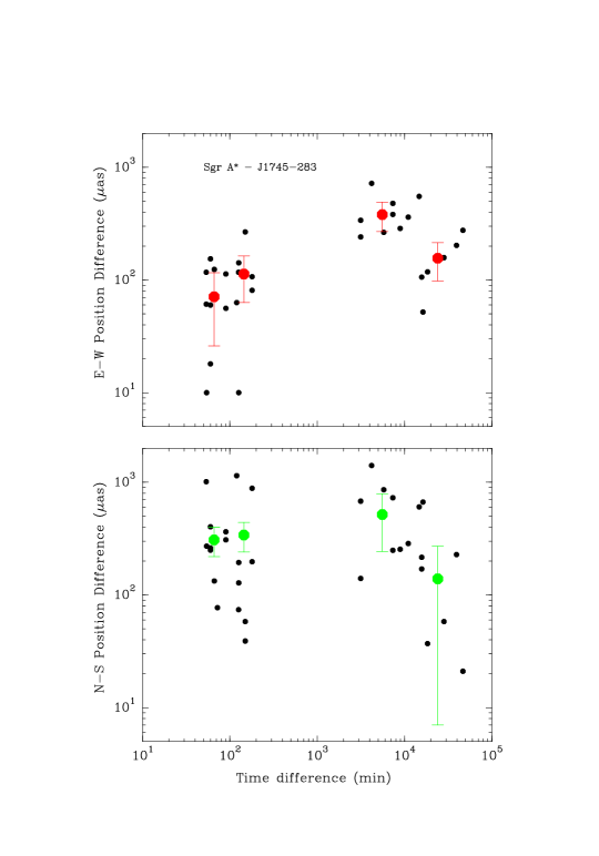
Figure 2: Position wander of Sgr A*. Plotted are East-West (top panel) and North-South (bottom panel) position differences as a function of time separation. Also shown are binned average position differences as large points with error bars. These position differences are likely caused by uncompensated atmospheric path-delay errors and should be considered as upper limits to the position wander of Sgr A*.

2.2 Position wander: days to weeks

The position wander of Sgr A* on time scales of days to weeks was determined from “daily” position measurements, obtained from $\approx 5$ hours of data when source elevations were above $\approx 20^{\circ}$ at most of the five inner-VLBA antennas. These positions were plotted in Fig. 3 of Reid & Brunthaler (2004), after removing the long-term proper motion of Sgr A* of $6.379$ mas yr^-1 along a position angle of $209.60^{\circ}$ East of North. We differenced the EW and NS positions for all pairs of measurements separated by less than $10^{5}$ min; the magnitudes of these position differences are shown in Fig. 2, along with weighted averages for two time-bins.

The average difference in EW position for measurements separated by $\approx 6000$ min ($\approx 4$ days) is about $400~{}\mu{\rm as}$. This difference is likely not a property of the emission of Sgr A*; instead it is probably caused by mis-modeling large-scale propagation delays through the Earth’s atmosphere. Most of the data used in this analysis were collected before we started to measure atmospheric path-lengths in 2003. Without this calibration, residual zenith path-length errors of $\sim 5$ cm are typical for the VLBA correlator model at 7-mm wavelength. Since propagation delays can be correlated with large-scale weather patterns, which have characteristic time scales of several days, one expects to see such a residual signature in our position differences.

3 Constraints upon hot-spot models of Sgr A* variability

Limits upon the variability in the centroid position of high resolution images of Sgr A* imply a constraint upon orbiting hot-spot models for Sgr A*’s radio variability. This will necessarily be a function of the hot-spot orbit and the hot-spot/disk flux ratio. In this section we derive the expected variability for two simple hot-spot models. The first is an optically thin Newtonian hot-spot, while the second fully incorporates general relativity and the opacity of a disk constructed such that it reproduces the observed spectrum of Sgr A*.

3.1 Idealized Newtonian hot-spot centroid variability

For the idealized Newtonian hot-spot we assume that there is no lensing by the black hole, the disk is completely optically thin, and the hot-spot is a point (the first two are physically appropriate for spots at large orbital radii). In this case the hot spot’s orbit (which we assume to be circular with radius $r$) is simply given by Kepler’s law:

$$x(t)=r\cos(\Omega t+\phi)\,\quad y(t)=r\cos i\sin(\Omega t+\phi)\,$$ (1)

where $i$ is the orbital inclination,

$$\Omega=\sqrt{\frac{GM_{\rm SgrA*}}{r^{3}}}\,,$$ (2)

$M_{\rm SgrA*}$ is the mass of Sgr A*, and $\phi$ is an arbitrary phase.

The image centroid, $\mbox{\boldmath$\rm X$}_{C}$ is constructed by integrating the source emission over a time $T$, which need not be small in comparison to the orbital period, and thus the motion of the hot-spot will generally be important. Explicitly, if we set the centroid of the disk emission to be at the origin,

$$\mbox{\boldmath$\rm X$}_{C}=\frac{\int_{0}^{T}F_{\rm spot}(t)\mbox{\boldmath$\rm x$}(t)dt}{\int_{0}^{T}\left[F_{\rm disk}+F_{\rm spot}(t)\right]dt}\,.$$ (3)

This will generally be a function of the initial phase of the orbit, $\phi$, and the integration time $T$. If we make the simplifying assumption that the hot-spot flux may be treated as roughly constant, then this reduces to

$$\mbox{\boldmath$\rm X$}_{C}=\eta\overline{\mbox{\boldmath$\rm x$}}(\phi;T)\quad\text{where}\quad\eta\equiv\frac{F_{\rm spot}}{F_{\rm disk}+F_{\rm spot}}\,,$$ (4)

and $\overline{x}(\phi;T)$ is the average spot position over some time $T$ with initial orbital phase $\phi$. It is straightforward to show that

$$\displaystyle\overline{x}(\phi;T) = \displaystyle r~{}{\rm sinc}\left(\frac{\Omega T}{2}\right)\cos\phi$$

$$\displaystyle\overline{y}(\phi;T) = \displaystyle r~{}{\rm sinc}\left(\frac{\Omega T}{2}\right)\cos i\sin\phi\,,$$ (5)

where a factor of $\Omega T/2$ has been subsumed into the arbitrary phase $\phi$. This corresponds to a single observation of the position of Sgr A*.

To study the position wander, we must compare two such measurements separated by some time $\Delta T$. This results in a change in the centroid position of

$$\displaystyle\left|\Delta\mbox{\boldmath$\rm X$}_{C}\right|(\phi;T,\Delta T)=\eta\left|\overline{\mbox{\boldmath$\rm x$}}(\phi+\Omega\Delta T;T)-\overline{\mbox{\boldmath$\rm x$}}(\phi;T)\right|$$

$$\qquad=\displaystyle\eta~{}r~{}{\rm sinc}\left(\frac{\Omega T}{2}\right)\sin\left(\frac{\Omega\Delta T}{2}\right)$$

$$\qquad\qquad\qquad\displaystyle\times\sqrt{\cos^{2}\phi+\cos^{2}i\sin^{2}\phi}\,.$$ (6)

Maximizing the position wander over the arbitrary initial phase simply removes the terms in the radical:

$$\left|\Delta\mbox{\boldmath$\rm X$}_{C,\rm max}\right|(T,\Delta T)=\eta~{}r~{}{\rm sinc}\left(\frac{\Omega T}{2}\right)\sin\left(\frac{\Omega\Delta T}{2}\right)\,.$$ (7)

While it may be unlikely that any given observation of the position wander will allow detection of the maximum centroid displacement, this quantity places a strict constraint upon hot-spots. Alternatively, one may wish to compare the observations to the predicted RMS centroid variability, which in this case is roughly $70\%$ of $\left|\Delta\mbox{\boldmath$\rm X$}_{C,\rm max}\right|(T,\Delta T)$.

For fixed $T$ and $\Delta T$, $\left|\Delta\mbox{\boldmath$\rm X$}_{C,\rm max}\right|$ vanishes when an integral number of periods is commensurate with either the integration time (and thus $\overline{\mbox{\boldmath$\rm x$}}(\phi;T)$ vanishes identically) or the delay between measurements. These are evident in Figure 3, in which the thin blue line shows $\left|\Delta\mbox{\boldmath$\rm X$}_{C,\rm max}\right|$ as a function of orbital period for a number of values of $\eta$ with $T=1\,{\rm hr}$ and $\Delta T=4\,{\rm hr}$. However, by choosing many different $T$ and $\Delta T$, it is possible fill in the nulls associated with each individual choice. There will be constraints upon what values of $T$ and $\Delta T$ are possible, e.g., due to sensitivity and imaging requirements (see §2). The upper-envelope of the observed centroid displacement for $1\,{\rm hr}\leq T\leq 4\,{\rm hr}$ and $1\,{\rm hr}\leq\Delta T\leq 4\,{\rm hr}$ is shown in Fig. 3 by the thick, solid blue line. For reference we also show, with dotted blue lines, the maximum deviation possible, corresponding to the case when all of the flux is due to the hot spot.

Generally, the observed displacement has a maximum near orbital periods of roughly $\pi\sqrt{T\Delta T}$. That such a maximum must exist can be inferred from the facts that (i) at large orbital radii the Keplerian velocity decreases and thus beyond some distance the hot spot will move sufficiently slow as to produce no detectable change in it’s position over the time $\Delta T$, and (ii) at small orbital radii the intrinsic variability in the spot position is smaller and the hot-spot makes many complete orbits in the integration time $T$, and thus the variable portion of the centroid position is dominated by a small fraction of the integrated flux, yielding again a small observable change in the centroid position. However, we may also show this explicitly by considering the asymptotic expansions of eq. (7). For small $\Omega$ (large period $P$), the ${\rm sinc}$-term is roughly unity and

$$\left|\Delta\mbox{\boldmath$\rm X$}_{C,\rm max}\right|(T,\Delta T)=\eta r\frac{\Omega\Delta T}{2}\propto r^{-1/2}\,.$$ (8)

In contrast, for large $\Omega$, $\left|\Delta\mbox{\boldmath$\rm X$}_{C,\rm max}\right|(T,\Delta T)$ is strongly oscillatory. Nevertheless, it is bounded from above by the ${\rm sinc}$ term, and thus

$$\left|\Delta\mbox{\boldmath$\rm X$}_{C,\rm max}\right|(T,\Delta T)\leq\frac{2\eta r}{\Omega T}\propto r^{5/2}\,.$$ (9)

Setting these limiting expressions equal to each other gives the desired condition that a maximum observed displacement occurs near $\Omega\simeq 2/\sqrt{T\Delta T}$. Note that this is true for the envelope obtained by varying $T$ and $\Delta T$ in the prescribed ranges as well, and serves as a simple estimate of the sensitivity of these types of measurements.

3.2 Fully relativistic, hot-spot in an optically thick disk

We now consider a more realistic model in which a hot spot is embedded in an accretion disk, including the relativistic beaming, Doppler boosting, strong gravitational lensing and the opacity of the disk and hot spot. This is necessarily a more complicated model, and thus we address it numerically via the ray-tracing, radiative-transfer code described in Broderick & Loeb (2006) (to which we direct the reader for more information, the model only being summarized below).

Due to its ability to shield the hot spot from view, the structure of the background disk is of particular importance. In the absence of an unambiguous prediction from existing accretion flow theory, we have modeled it as a self-similar Radiatively Inefficient Accretion Flow (RIAF) following Yuan et al. (2003). Specifically, the accretion flow is characterized by a Keplerian velocity distribution, a population of thermal electrons with density and temperature

$$n_{e,\rm th}=n^{0}_{e,\rm th}r^{-1.1}{\rm e}^{-z^{2}/2\rho^{2}}\quad\text{and}\quad T_{e}=T^{0}_{e}r^{-0.84}\,,$$ (10)

respectively, a population of non-thermal electrons

$$n_{e,\rm nth}=n^{0}_{e,\rm nth}r^{-2.9}{\rm e}^{-z^{2}/2\rho^{2}}\,,$$ (11)

and spectral index $\alpha_{\rm disk}=1.25$ (defined as $S\propto\nu^{-\alpha}$), and a toroidal magnetic field in approximate ($\beta=10$) equipartition with the ions (which produce the majority of the pressure), i.e.,

$$\frac{B^{2}}{8\pi}=\beta^{-1}n_{e,\rm th}\frac{m_{p}c^{2}}{6r}\,.$$ (12)

In all expressions $r$, $\rho$ and $z$ are measured in units of $GM_{\rm SgrA*}/c^{2}$. The power-laws are taken from Yuan et al. (2003), and the three coefficients ($n^{0}_{e,\rm th}$, $T^{0}_{e}$ and $n^{0}_{e,\rm nth}$) are set by fitting the radio, sub-mm and near-infrared spectrum of Sgr A*. While this is not a unique model for the accretion flow around Sgr A*, it is representative of the general class of RIAFs, and we expect that our results will be quite generic.

The hot-spot is modeled by a spherical (in it’s frame) Gaussian over-density of non-thermal electrons, with a radial scale of $1.5GM_{\rm SgrA*}/c^{2}$. The primary distinction between the systems shown in the panels of Fig. 3 is the size of the photosphere of the hot-spot ($\delta r$), larger hot-spots necessarily being more luminous.

The radiative transfer is assumed to be dominated by synchrotron emission and absorption. We follow Jones & O’Dell (1977) for the power-law electron distributions in the accretion flow and the hot spot, cutting the electron distributions off below Lorentz factors of $10^{2}$, roughly in agreement with the assumptions in Yuan et al. (2003). We treat the radiative transfer of the thermal component of the accretion flow in a similar fashion as that discussed in Yuan et al. (2003), appropriately altered to account for the relativistic nature of the bulk motion (see, e.g., Broderick & Blandford 2004 for more detail on how this may be done).

The centroid displacements were computed by (i) generating a sequence of images associated with an entire orbit, (ii) determining the instantaneous image centroid for each, (iii) inserting these into eq. (3) to determine the time-integrated centroid position for a given $T$, and finally (iv) given a $\Delta T$ varying the orbital phase until the maximum $\left|\Delta\mbox{\boldmath$\rm X$}_{C,\rm max}\right|(T,\Delta T)$ was obtained. The result for $T=1\,{\rm hr}$ and $\Delta T=4\,{\rm hr}$ is shown by the thin green line in Fig. 3, and exhibits many of the features found in the idealized Newtonian case. This procedure was repeated a number of times for randomly chosen $T\in[1\,{\rm hr},4\,{\rm hr}]$ and $\Delta T\in[1\,{\rm hr},4\,{\rm hr}]$ to produce the upper-envelope of the centroid displacements, and is shown by the thick green line in Fig. 3.

The primary effect is the suppression of the centroid variability due to the opacity of the background accretion flow. This suppression becomes substantial at radii near the location of the photosphere, which is approximately $12.5GM_{\rm SgrA*}/c^{2}$ at $7\,{\rm m}{\rm m}$ wavelength. In contrast, at large orbital radii the idealized Newtonian model fits quite well. This interpretation is further supported by the fact that the idealized Newtonian model fits quite well once it has been modified to include opacity. Specifically, as a rough approximation, we reduce the hot-spot flux by a factor of ${\rm e}^{-\tau}$, where

$$\tau=\left(\frac{r+\delta r}{12.5}\right)^{-2.99}\propto rn_{e,\rm nth}B^{\alpha_{\rm disk}+3/2}$$ (13)

is the optical depth associated with the non-thermal electrons in the accretion flow. This is shown by the magenta lines in Fig. 3. While we should also include the thermal electron component, at $7\,{\rm m}{\rm m}$ wavelength the non-thermal electrons appear to dominate the opacity.

The free parameter $\delta r$ is associated with the finite extent of the hot spot. That is, it is possible for the spot to be visible even if the hot-spot center is inside of the accretion-flow photosphere. It is for this reason that the centroid variability is more similar to the idealized Newtonian value for high-luminosity spots than for low-luminosity spots. Setting $\delta r$ using the hot-spot photosphere radius alone gives the dotted magenta line, which underestimates the centroid variability considerably at small radii for large (bright) hot spots. This is due to the failure of the idealized Newtonian calculation to account for the strong lensing of large spots in small orbits (with $r_{\rm spot}\simeq r$). However, simply employing a larger $\delta r$ (64% larger at the largest disk/hot-spot flux ratio we consider) results in a substantially improved fit.

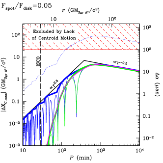
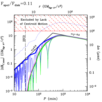
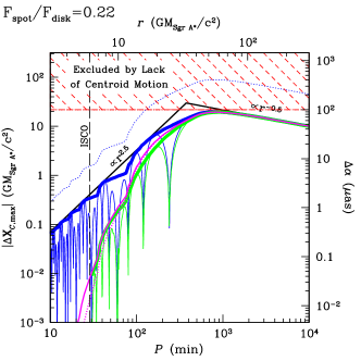
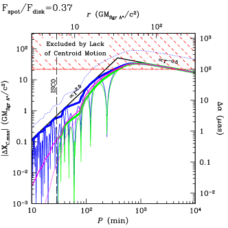
Figure 3: Maximum observed physical displacement of the centroid as a function of the orbital period for the idealized Newtonian case (blue) and the fully general relativistic case appropriate for Sgr A* (green) for a number of spot-disk flux ratios. The period and angular offset scales assume a distance of 8.0 kpc and M${}_{SgrA*}=4\times 10^{6}$ M_⊙. The thin blue and green lines show the variation associated with an observations integrated over $T=1\,{\rm hr}$ and separated by $\Delta T=4\,{\rm hr}$. The thick blue and green lines show the envelope for all observation strategies with $T\geq 1\,{\rm hr}$ and $\Delta T\leq 4$. In all cases the thin dotted blue line shows the maximum deviation possible, corresponding to when all of the flux is due to the hot spot. The solid black lines show the asymptotic power-law behavior at both short and long periods. The dotted and solid magenta lines shows the opacity modified idealized Newtonian case without and with lensing, respectively. Finally, the regions excluded by $7\,{\rm m}{\rm m}$ VLBI are shown by the red hatched regions. For convenience the orbital radii and angular scale of the centroid displacements are shown on the top and right axes, respectively.

4 Discussion

Possible reasons for position wander include intrinsic variations in the position of the emitting plasma (e.g., variations in the accretion flow or perhaps in a jet) or extrinsic processes such as refractive interstellar scattering. Sgr A* is observed to be diffractively scattered to a size of $\theta_{sc}\sim 0.5(\lambda/0.7~{}{\rm cm})^{2}$ mas, where $\lambda$ is the observing wavelength. Flux density fluctuations are modest and decrease in strength with increasing wavelength; thus strong refractive scintillations are not indicated (Gwinn et al. 1991). Any refractive position wander should be $\ll\theta_{sc}$ and should occur on time scales $>\theta_{sc}D/v$, where $D$ is the distance and $v$ is the transverse velocity of the scattering “screen” relative to the observer (Romani, Narayan & Blandford 1986). For $D\approx R_{0}\approx 8$ kpc (Reid 1993) and $v\sim 100$ km s^-1, characteristic of material in the inner $\sim 100$ pc of the Galaxy where large scattering sizes are observed, the refractive time scale is $>10^{3}$ hours. Thus, we would not expect a significant contribution to the short-term wander of Sgr A* from refractive scattering. For comparison, Gwinn et al. (1988), using VLBI observations of the Sgr B2(N) H₂O masers near the Galactic center, find a wander limit of $<18~{}\mu{\rm as}$ over timescales of months for maser spots, which are diffractively scattered to a comparable size (at 22 GHz) as Sgr A* (at 43 GHz). Of course, our results provide an observation limit to any refractive position wander.

Since extrinsic sources of position wander (scattering) are unlikely to be dominant, we now discuss the implications for intrinsic wander from variations in brightness within an accretion disk given in §3. Our observations of the lack of short-term wander of the centroid position of Sgr A* presented in §2.1 give an upper limit of $\approx 100~{}\mu{\rm as}$ for time scales of $\approx 1~{}{\rm to}~{}4$ hours. This translates to an upper limit on the wander versus orbital period plots in Fig. 3 as indicated by the horizontal red line and hatched region. (In the very unlikely event that the accretion disk inclination is both near $90^{\circ}$ and oriented nearly North-South on the sky, we would need to use our NS limits, which are a factor of three weaker.) Our EW limit is below the dotted blue line in Fig. 3, which is for hot spot flux density dominating over disk (or possible jet) emission, for orbital periods exceeding 120 min (corresponding to orbital radii larger than $15\,GM_{\rm SgrA*}/c^{2}$ for $M_{\rm SgrA*}=4\times 10^{6}$ M_⊙). For cases in which the hot spot flux density is weaker than that of the disk, somewhat longer periods are allowed. For example, for $F_{\rm spot}/F_{\rm disk}=0.37$, orbital periods longer than 5 hr are excluded.

In practice, the limits placed by current $7\,{\rm m}{\rm m}$ VLBI are significantly weaker. The limited sensitivity to hot spots on compact orbits is primarily due to two reasons: (1) “long” integration times ($T\gtrsim 1\,{\rm hr}$) average much of the short time variability out, and (2) the opacity of the accretion flow itself makes it difficult to view hot-spots on compact orbits at $7\,{\rm m}{\rm m}$. The integration time is limited by the sensitivity issues and the small number of antennas yielding interferometer baselines $<1500$ km afforded by the current VLBA; higher bandwidth recording in the future should help alleviate this problem. The optical depth is a property of Sgr A* itself, and can only be addressed by observations at shorter wavelengths. However, even in the absence of an optically thick accretion flow, it is not possible to increase the centroid variability by more than an order of magnitude due to the intrinsically small orbital radii, as seen by comparing the blue and green limits in the lower-left panel of Fig. 3.

Nevertheless, high-resolution astrometry is reaching sensitivities and resolutions sufficient to begin to test the hot-spot model for bright Sgr A* flares. Unfortunately, the typical fractional variability at $7\,{\rm m}{\rm m}$ during our observations was roughly $\pm 20\%$, implying that significant improvement in positional accuracy will be required to constrain such events. Since the observed centroid wander is consistent with systematic errors, owing predominantly to centimeter-scale errors in the modeling of the atmospheric path-delays, substantially increasing accuracy will require better calibration techniques. However, for the somewhat rare instances in which the spot is substantially brighter (Zhao, Bower & Goss 2001), the VLBA at 7, or possibly 3, mm wavelength appears poised to provide significant limits upon the existence and morphology of inhomogeneities in the accretion flow surrounding Sgr A*.

Ultimately, observations at $\sim 1$ mm wavelength with VLBI techniques or at infrared wavelengths with an instrument like GRAVITY (Gillessen et al. 2006) may be necessary to image the region within $\sim 3$ Schwarzschild radii on the short time scales needed to test the hot-spot model.

A.B. is supported by the Priority Programme 1177 of the Deutsche Forschungsgemeinschaft.

Facilities: VLBA

References

- see, e.g., Bower et al. (2004) Bower, G. C., Falcke, H., Herrnstein, R. M., Zhao, J.-H., Goss, W. M. & Backer, D. C. 2004, Science, 304, 704
- Broderick & Blandford (2004) Broderick, A. & Blandford, R., 2004, MNRAS, 349, 994
- Broderick & Loeb (2005) Broderick, A. E. & Loeb, A., 2005, MNRAS, 363, 353
- Broderick & Loeb (2006) Broderick, A. E. & Loeb, A., 2006, MNRAS, 267, 905
- Dehnen & Binney (1998) Dehnen, W. & Binney, J. J 1998, MNRAS, 298,387
- Ghez et al. (2003) Ghez, A. M. et al.2003, ApJ, 586, L127
- Gillessen et al. (2006) Gillessen et al.2006, SPIE, 6268, 33
- Gwinn et al. (1988) Gwinn, C. R., Moran, J. M., Reid, M. J. & Schneps, M. H. 1988, ApJ, 330, 817
- Gwinn et al. (1991) Gwinn, C. R., Danen, R. M., Middleditch, J., Ozernoy, L. M. & Tran, T. KH. 1991, ApJ, 381, L43
- Jones & O’Dell (1977) Jones, T. W. & O’Dell, S. L., 1977, ApJ, 214, 522
- Menten et al. (1997) Menten, K. M., Reid, M. J., Eckart, A. & Genzel, R. 1997, ApJ, 475, L111
- Reid (1993) Reid, M. J. 1993, ARA&A, 31, 345
- Reid et al. (1999) Reid, M. J., Readhead, A. C. S., Vermeulen, R. C. & Treuhaft, R. N. 1999, ApJ, 524, 816
- Reid et al. (2003) Reid, M. J., Menten, K. M., Genzel, R., Ott, T., Schödel, R. & Eckart, A. 2003, ApJ, 587, 208
- Reid & Brunthaler (2004) Reid, M. J. & Brunthaler, A. 2004, ApJ, 616, 872
- Romani, Narayan & Blandford (1986) Romani, R. W., Narayan, R. & Blandford, R. 1986, MNRAS, 220, 19
- Schödel et al. (2002) Schödel, R. et al.2002, Nature, 419, 694
- Yuan et al. (2003) Yuan, F., Quataert, E. & Narayan, R., 2003, ApJ, 598, 301
- Zhao, Bower & Goss (2001) Zhao, J.-H., Bower, G. C. & Goss, W. M. 2001, ApJ, 547, L29