Abstract

In the beginning of the 1950’s, Wigner introduced a fundamental deformation from the canonical quantum mechanical harmonic oscillator, which is nowadays sometimes called a Wigner quantum oscillator or a parabose oscillator. Also, in quantum mechanics the so-called Wigner distribution is considered to be the closest quantum analogue of the classical probability distribution over the phase space. In this article, we consider which definition for such distribution function could be used in the case of non-canonical quantum mechanics. We then explicitly compute two different expressions for this distribution function for the case of the parabose oscillator. Both expressions turn out to be multiple sums involving (generalized) Laguerre polynomials. Plots then show that the Wigner distribution function for the ground state of the parabose oscillator is similar in behaviour to the Wigner distribution function of the first excited state of the canonical quantum oscillator.

Keywords: Wigner distribution function, non-canonical quantum mechanics, phase space, parabose oscillator
Running head: Wigner d.f. for the parabose oscillator

1 Introduction

The harmonic oscillator is one of the most appealing models due to its well known solutions in classical mechanics and in quantum mechanics, and due to a wide variety of applications in various branches of physics [1]. In classical mechanics its solution is unique, and so it is in the canonical non-relativistic treatment in quantum mechanics [2]. In this quantum approach, the position and momentum operators ($\hat{p}$ and $\hat{q}$, respectively) satisfy the canonical commutation relation $[{\hat{p},\hat{q}}]=-i\hbar$, and the model is described by its Hamiltonian $\hat{H}$ and the Heisenberg equations. This algebraic description can be translated to a description by means of wave functions. In the position representation, for example, the operator $\hat{q}$ corresponds to multiplying functions by the variable $q$ and the Heisenberg operator equations correspond to Schrödinger’s equation, the solutions of which are expressed through Hermite polynomials. These solutions or wave functions lead to important position probability functions.

To study the applicability of a system modelled by a harmonic oscillator, one often turns to expressions for the joint quasi-probability function of momentum and position, i.e. to a quantum analogue of phase space. The Wigner distribution function (d.f.) [3] is the main theoretical tool here, as it is considered as the closest quantum analogue of a classical distribution function over the phase space. The quantum harmonic oscillator is one of the first systems for which the Wigner d.f. was computed analytically. Nowadays, there are also advanced experimental techniques that enable one to measure phase space densities for certain quantum systems [4, 5], and thus compare theoretical results with experimental results [6, 7, 8].

It is in this context that certain deformations or generalizations of the quantum harmonic oscillator are of relevance. In particular, deformations that are still exactly solvable and for which the Wigner d.f. can be computed analytically are highly interesting. One such model is the $q$-deformed quantum harmonic oscillator, being exactly solvable [9, 10, 11] and having found applications in various physical models [12]. Its Wigner d.f. has been computed in [13].

A deformation or generalization of the canonical quantum harmonic oscillator that is more fundamental in nature was proposed by Wigner [14]. It is known as the one-dimensional Wigner quantum oscillator or as the parabose oscillator. In Wigner’s approach, the canonical commutation relations are not assumed. Instead of that, the compatibility of Hamilton’s equations and the Heisenberg equations is required. This approach has been the fundamental starting point of so-called Wigner Quantum Systems [15]. In such an approach, one typically obtains several solutions (several algebraic representations), of which only one corresponds to the canonical solution. It is thus a natural and fundamental extension of canonical quantum mechanics. It is also of growing importance as deviations from the canonical commutation relations (in particular of commuting position operators in the context of non-commutative quantum mechanics) are supported by investigations from several field [16, 17, 18, 19].

The one-dimensional Wigner quantum oscillator itself was already solved by Wigner [14], leading to an oscillator energy spectrum similar to the canonical one but with shifted ground state energy equal to some arbitrary positive number $a$. In a sense, this number $a$ can be considered as the deformation parameter, and the solutions of the Wigner quantum oscillator reduce to the canonical one when $a=1/2$. Wigner’s formulation was also the inspiration for the introduction of parabosons (and parafermions), as the common boson commutator relation of the canonical case is, in Wigner’s approach, replaced by a triple relation that is also the defining relation of a paraboson [20]. Later on, one realized that Lie superalgebras are the natural framework for this algebraic description [21], and in particular that the representations of the Wigner quantum oscillator are in one-to-one correspondence with the unitary irreducible lowest weight representations of the Lie superalgebra $\mathfrak{osp}(1|2)$.

So the Wigner quantum oscillator, being the generalization of the canonical one, could play an important role to explain various phenomena more precisely, and its importance is undeniable. However, so far its application has been restricted in comparison with the canonical harmonic oscillator due to the fact that its behaviour in phase space has not been studied. In other words, there is no expression of the joint quasi-probability distribution function (Wigner d.f.) of position and momentum available for the Wigner quantum oscillator. The main problem is that the treatment a Wigner d.f. usually starts from the assumption that the commutator of $\hat{p}$ and $\hat{q}$ is a constant, which is no longer the case for the non-canonical Wigner quantum oscillator. It is precisely this problem which is being tackled and solved here.

In this paper, we first recall some basic facts of the one-dimensional Wigner quantum oscillator or parabose oscillator. The emphasis is on the algebraic description, in terms of the Lie superalgebra $\mathfrak{osp}(1|2)$ and representations characterized by a positive real number $a$ (section 2). In section 3 we discuss the main definition of the Wigner d.f. in the current non-canonical setting. The main part of the paper is devoted to computing the Wigner d.f. $W_{n}(p,q)$ analytically, for the parabose oscillator in the $n$th excited pure state $|n\rangle$. For $n=0$ (and $n=1$), the calculation is somewhat simpler than in the general case, and this is treated first in section 4. The calculation involves various computational tools. In some steps, series are term wise integrated, so one should pay attention to convergence. Here, we shall often assume that the parameter $a$ is of the form $a=1/2+m$, with $m$ a nonnegative integer; in that case all series appearing are finite and there are no convergence problems. The final expression of $W_{0}(p,q)$ is essentially a series in terms of Laguerre polynomials, depending only upon $p^{2}+q^{2}$, or alternatively a confluent hypergeometric series in $p^{2}+q^{2}$, see (33). Section 5 then deals with the general case: the computation of $W_{n}(p,q)$. Here, the analysis is quite involved, and some intermediate calculations are performed in an Appendix B. We obtain two alternative expressions for $W_{n}(p,q)$, (39) and (41), both as series of Laguerre polynomials in $p^{2}+q^{2}$. Section 6 deals with some plots of the newly obtained Wigner distribution functions, discusses some properties and summarizes some conclusions.

To end the introduction, let us introduce some of the notation and classical results we are going to use. Many of the formulas encountered in this article will involve binomial coefficients, factorials etc. It is therefor convenient to use the notation for (generalized) hypergeometric series [22]. Let $r$ and $s$ be nonnegative integers, a hypergeometric series with $r$ numerator and $s$ denominator parameters is then defined as

$${}_{r}F_{s}\left(\genfrac{}{}{0.0pt}{}{a_{1},\ldots,a_{r}}{b_{1},\ldots,b_{s}};z\right)=\sum_{k\geq 0}\frac{(a_{1},\ldots,a_{r})_{k}}{(b_{1},\ldots,b_{s})_{k}}\frac{z^{k}}{k!},$$ (1)

where

$$(a_{1},\ldots,a_{r})_{k}=(a_{1})_{k}(a_{2})_{k}\cdots(a_{r})_{k},\ \text{and}\ (a)_{k}=\frac{\Gamma(a+k)}{\Gamma(a)}=a(a+1)\cdots(a+k-1)$$ (2)

is the rising factorial or Pochhammer symbol. When one of the numerator parameters $a_{j}$ is a negative integer, the series is terminating and in fact a polynomial in $z$. Of course, if one of the denominator parameters is also a negative integer, it has to be “more negative” such that the numerator vanishes before the denominator does.

All classical orthogonal polynomials can be written using this hypergeometric notation. In particular one has for the Laguerre polynomials [23]:

$$L_{n}^{(\alpha)}(z)=\frac{(\alpha+1)_{n}}{n!}\,{}_{1}F_{1}\left(\genfrac{}{}{0.0pt}{}{-n}{\alpha+1};z\right)=\frac{(\alpha+1)_{n}}{n!}\,{}_{1}F_{1}(-n;\alpha+1;z).$$ (3)

Here, we also introduced an alternative notation for the confluent hypergeometric series ${}_{1}F_{1}$. If the parameter $\alpha$ is $0$, we will simply write $L_{n}(z)$ instead of $L_{n}^{(0)}(z)$. Often, the $L_{n}(z)$ are called Laguerre polynomials, while the $L_{n}^{(\alpha)}$ are called the generalized Laguerre polynomials. For the classical orthogonality of the Laguerre polynomials to hold $\alpha$ needs to be bigger than $-1$. In particular, if $\alpha$ is a negative integer, the definition (3) is no longer valid since one has a negative integer appearing as a denominator parameter. The Laguerre polynomials can be written in an alternative way such that they are defined for all values of $\alpha$:

$$L_{n}^{(\alpha)}(z)=\frac{1}{n!}\sum_{k=0}^{n}\frac{(-n)_{k}(\alpha+k+1)_{n-k}}{k!}z^{k}.$$ (4)

Many well known summation formulas can be very neatly expressed using the hypergeometric notation. Most notable are the binomial summation theorem:

$${}_{1}F_{0}({a};{\ };z)=(1-z)^{-a},$$ (5)

with $|z|<1$ if $a$ is not a negative integer, and the Chu-Vandermonde summation theorem for a terminating Gauss hypergeometric series:

$${}_{2}F_{1}\left(\genfrac{}{}{0.0pt}{}{-n,a}{c};1\right)=\frac{(c-a)_{n}}{(c)_{n}},$$ (6)

with $n$ a nonnegative integer. There exists also a very extensive theory of hypergeometric transformations, a very important transformation being Kummer’s transformation for confluent hypergeometric series:

$${}_{1}F_{1}(b;c;z)=e^{z}\,{}_{1}F_{1}(c-b;c;-z).$$ (7)

2 The one-dimensional parabose oscillator

In this paragraph we briefly describe the treatment of a harmonic oscillator as a Wigner quantum system. Although first introduced by Wigner almost 60 years ago, and described in some articles and book chapters, it may still be useful to recall the main results.

Consider the Hamiltonian for a one-dimensional harmonic oscillator (in units with mass and frequency both equal to 1):

$$\hat{H}=\frac{\hat{p}^{2}}{2}+\frac{\hat{q}^{2}}{2},$$ (8)

where $\hat{p}$ and $\hat{q}$ denote respectively the momentum and position operator of the system. Wigner [14] already noted that there are other solutions besides the canonical one if one only requires the compatibility between the Hamilton and the Heisenberg equations. Thus, one drops the canonical commutation relation $[\hat{p},\hat{q}]=-i$ (we have taken $\hbar=1$), and instead one imposes the equivalence of Hamilton’s equations

$$\dot{\hat{p}}=-\frac{\partial H}{\partial q},\quad\dot{\hat{q}}=\frac{\partial H}{\partial p}$$

and the Heisenberg equations

$$\dot{\hat{p}}=i[\hat{H},\hat{p}],\quad\dot{\hat{q}}=i[\hat{H},\hat{q}].$$

Expressing this equivalence leads to the following compatibility conditions:

$$[\hat{H},\hat{p}]=i\hat{q},\quad[\hat{H},\hat{q}]=-i\hat{p}.$$ (9)

So, one has to find operators $\hat{p}$ and $\hat{q}$, acting in some Hilbert space, such that the compatibility conditions (9) hold, with $\hat{H}$ given by (8). Also, in this Hilbert space $\hat{p}$ and $\hat{q}$ have to be self-adjoint.

The solutions to (9) can be found by introducing two new (yet unknown) operators $\hat{b}^{+}$ and $\hat{b}^{-}$:

$$\hat{b}^{\pm}=\frac{1}{\sqrt{2}}(\hat{q}\mp i\hat{p}),$$ (10)

or equivalently

$$\hat{q}=\frac{1}{\sqrt{2}}(\hat{b}^{+}+\hat{b}^{-}),\quad\hat{p}=\frac{i}{\sqrt{2}}(\hat{b}^{+}-\hat{b}^{-}).$$

It is then easily checked that

$$\hat{H}=\frac{1}{2}\{\hat{b}^{-},\hat{b}^{+}\},$$ (11)

and that the compatibility conditions (9) are equivalent with

$$[\{\hat{b}^{-},\hat{b}^{+}\},\hat{b}^{\pm}]=\pm 2\hat{b}^{\pm}.$$ (12)

The relations (12) are in fact the defining relations of one pair of parabose operators $\hat{b}^{\pm}$ [20]. Moreover, from the self-adjointness of the position and momentum operators it follows that

$$(\hat{b}^{\pm})^{\dagger}=\hat{b}^{\mp}.$$ (13)

It is known that the Lie superalgebra generated by two odd elements $\hat{b}^{\pm}$ subject to the restriction (12) is the Lie superalgebra $\mathfrak{osp}(1|2)$ [21]. So, the solutions to our problem are given by the star representations of the Lie superalgebra $\mathfrak{osp}(1|2)$. These are known, and are characterized by a positive real number $a$ and a vacuum vector $|0\rangle$, such that

$$\hat{b}^{-}|0\rangle=0,\quad\{\hat{b}^{-},\hat{b}^{+}\}|0\rangle=2a|0\rangle.$$

The representation space can then be shown to be the Hilbert space $\ell^{2}(\mathbb{Z}_{+})$ with orthonormal basis vectors $|n\rangle$ ($n\in\mathbb{Z}_{+}$) and with the following actions:

$$\hat{b}^{+}|2n\rangle =\sqrt{2(n+a)}\,|2n+1\rangle, \hat{b}^{-}|2n\rangle =\sqrt{2n}\,|2n-1\rangle,$$ (14)

$$\hat{b}^{+}|2n+1\rangle =\sqrt{2(n+1)}\,|2n+2\rangle, \hat{b}^{-}|2n+1\rangle =\sqrt{2(n+a)}\,|2n\rangle,$$

from which it immediately follows that

$$\{\hat{b}^{-},\hat{b}^{+}\}|n\rangle=2(n+a)\,|n\rangle.$$ (15)

Using the actions (14), one can now compute the action of the commutator $[\hat{p},\hat{q}]$:

$$[\hat{p},\hat{q}]|2n\rangle=-2ai|2n\rangle,\quad[\hat{p},\hat{q}]|2n+1\rangle=-2(1-a)i|2n+1\rangle.$$ (16)

So the canonical commutation relations are only satisfied for $a=1/2$ and any representation with $a\neq 1/2$ thus leads to a non-canonical solution. It is also important to note that for such non-canonical solutions, the commutator $[\hat{p},\hat{q}]$ is not constant. This last fact has a serious impact on the computation of exponential operators involving linear combinations of $\hat{p}$ and $\hat{q}$ since the Baker-Campbell-Hausdorff theorem does not give rise to a simple formula.

The energy spectrum is now very easy to determine as well using (15) and (11):

$$\hat{H}|n\rangle=(n+a)\,|n\rangle,$$

so one has an equidistant energy spectrum with ground level given by $a$. This once again confirms that only $a=1/2$ yields the canonical solution.

Also the wave functions for the parabose oscillator in the position and momentum representation are known. Working in the position representation, the operator $\hat{q}$ is still represented by “multiplication by $q$”, the operator $\hat{p}$ however is no longer given by its canonical realization $-i\frac{d}{dq}$, but instead has a different realization with an extra term (depending on $a$) coming in. Using this realization the time-independent Schrödinger equation can then be solved yielding the following expressions for the orthonormal wave functions in terms of Laguerre polynomials [24, Chapter 23] and [25]:

$$\begin{split}\Psi_{2n}^{(a)}(q)&=(-1)^{n}\sqrt{\frac{n!}{\Gamma(n+a)}}\,|q|^{a-1/2}\,e^{-q^{2}/2}L_{n}^{(a-1)}(q^{2})\\ \Psi_{2n+1}^{(a)}(q)&=(-1)^{n}\sqrt{\frac{n!}{\Gamma(n+a+1)}}\,|q|^{a-1/2}\,e^{-q^{2}/2}qL_{n}^{(a)}(q^{2}).\end{split}$$ (17)

Again, for $a=1/2$, one recovers the very well known expression for the wave functions for a harmonic oscillator in terms of Hermite polynomials, since there are formulas relating $L_{n}^{(\mp 1/2)}(x^{2})$ to $H_{2n}(x)$ and $H_{2n+1}(x)$ respectively.

3 Distribution function for a non-canonical quantum system

A major advantage of the phase-space formulation of quantum mechanics is the fact than one is no longer dealing with operators, but instead with constant-number equations. More in particular, the expectation value of an arbitrary operator $\hat{A}(\hat{p},\hat{q})$ can be calculated using the distribution function $\Phi(p,q)$ as follows:

$$\mathrm{\mathop{Tr}}\{\hat{\rho}(\hat{p},\hat{q})\hat{A}(\hat{p},\hat{q})\}=\iint A(p,q)\Phi(q,p)\,dq\,dp,$$ (18)

with $A(p,q)$ the scalar function obtained by replacing the operators $\hat{p}$ and $\hat{q}$ in the expression for $\hat{A}(\hat{p},\hat{q})$ by scalar variables $p$ and $q$. Herein, $\hat{\rho}$ is the density operator, representing the state of the system. Also, both integrations run from $-\infty$ to $+\infty$; this will be the case for all integrations in this article.

It is also known that the distribution function $\Phi$ depends on the so-called correspondence rule used, this is, on the way one associates a function of non-commuting operators (thus an operator) to a given function of scalar variables. A very popular association rule is the Weyl correspondence, yielding as distribution function the so-called Wigner distribution function. Very often, the definition for the Wigner d.f. is written as follows:

$$W(p,q)=\frac{1}{2\pi}\int\langle q+\frac{\eta}{2}|\hat{\rho}|q-\frac{\eta}{2}\rangle e^{-i\eta p}d\eta.$$ (19)

This definition, however, is completely unsuitable for the case of non-canonical quantum mechanics, since it relies heavily on the canonical commutation relations. Indeed, it was shown by Tatarskii [26] (see also section 2.1 of Lee’s review paper [27]) that the Wigner d.f. defined by first principles (see equation (20) here) gives rise to expression (19) only if $\hat{p}$ and $\hat{q}$ satisfy $[\hat{p},\hat{q}]=-i$. So if the canonical commutation relations are not satisfied, one should go back to use this first principles approach, which is described in the rest of this section.

Another approach is the following [26]: is it clear that in order to define an association rule between functions of scalar variables $f(p,q)$ and operators $\hat{f}(\hat{p},\hat{q})$ it suffices to define this correspondence for the function $F(\lambda,\mu)=\exp(i(\lambda p+\mu q))$, with $\lambda$ and $\mu$ real variables. Indeed, an arbitrary analytical function $f(p,q)$ can be obtained from $F(\lambda,\mu)$ in the following way:

$$f(p,q)=f(\frac{1}{i}\frac{\partial}{\partial\lambda},\frac{1}{i}\frac{\partial}{\partial\mu})F(\lambda,\mu)\left|{}_{\lambda=\mu=0}\right..$$

Note that this expression is well-defined since the partial derivate operators commute. The operator corresponding to the function $f(p,q)$ under the chosen association rule, i.e. for the particular choice of $\hat{F}$, is then given by

$$\hat{f}(\hat{p},\hat{q})=f(\frac{1}{i}\frac{\partial}{\partial\lambda},\frac{1}{i}\frac{\partial}{\partial\mu})\hat{F}(\lambda,\mu)\left|{}_{\lambda=\mu=0}\right..$$

Once a choice for $\hat{F}$ is made, the corresponding distribution function $W_{F}$ may be calculated as follows:

$$W_{F}(p,q)=\frac{1}{4\pi^{2}}\iint\langle\psi|\hat{F}(\lambda,\mu)|\psi\rangle e^{-i(\lambda p+\mu q)}d\lambda d\mu,$$ (20)

where $\psi$ denotes the state of the system. This definition is independent of the canonical commutation relations and still allows the computation of averages by use of (18).

We now make the following choice for $\hat{F}$ [26, 27]:

$$\hat{F}(\lambda,\mu)=e^{i(\lambda\hat{p}+\mu\hat{q})}=e^{i\hat{X}},$$ (21)

where we have introduced the operator $\hat{X}$:

$$\hat{X}=\lambda\hat{p}+\mu\hat{q}.$$ (22)

Since this is the only correspondence rule we are using in this article, the subscript $F$ will be dropped from the notation. On the other hand, as we will be concentrating on calculating explicit expressions for the distribution function $W$ for the pure states $|n\rangle$, we will introduce the subscript $n$ to indicate this:

$$W_{n}(p,q)=\frac{1}{4\pi^{2}}\iint\langle n|e^{i\hat{X}}|n\rangle e^{-i(\lambda p+\mu q)}d\lambda d\mu.$$ (23)

Since in this article our goal will be to compute an explicit expression for (23), it is convenient to recall the expression for the Wigner d.f. $\tilde{W}_{n}$ in the case of canonical commutation relations:

$$\tilde{W}_{n}(p,q)=\frac{(-1)^{n}}{\pi}e^{-p^{2}-q^{2}}\,L_{n}(2p^{2}+2q^{2}),$$ (24)

where $L_{n}$ are the Laguerre polynomials. So, whatever result we obtain for $W_{n}$, replacing the parameter $a$ by $1/2$ should yield (24).

4 Wigner distribution function for the ground state and the first excited state

In this section, we compute an explicit expression for $W_{0}(p,q)$. This will already show the techniques involved in the computation of the Wigner d.f. for arbitrary states $|n\rangle$, but the resulting calculations are not quite so lengthy. To reiterate, the goal is to compute

$$W_{0}(p,q)=\frac{1}{4\pi^{2}}\iint\langle 0|e^{i\hat{X}}|0\rangle e^{-i(\lambda p+\mu q)}\,d\lambda d\mu.$$ (25)

Thus, obviously, in a first step we are going to determine the matrix elements $\langle 0|\exp(i\hat{X})|0\rangle$, and in a second step the integration will be performed.

The operator $\exp(i\hat{X})$ being defined as

$$e^{i\hat{X}}=\sum_{k\geq 0}\frac{i^{k}\hat{X}^{k}}{k!}$$

we first try to find $\langle 0|\hat{X}^{k}|0\rangle$. To this end, we write $\hat{X}=\lambda\hat{p}+\mu\hat{q}$ in terms of $\hat{b}^{\pm}$:

$$\hat{X}=\alpha^{+}\hat{b}^{+}+\alpha^{-}\hat{b}^{-}\ \text{with}\ \alpha^{\pm}=\frac{\mu\pm i\lambda}{\sqrt{2}}.$$ (26)

It is then immediately clear that

$$\langle 0|\hat{X}^{2k+1}|0\rangle=0$$ (27)

since an odd number of applications of $\hat{b}^{+}$ and $\hat{b}^{-}$ on $|0\rangle$ does not yield a term corresponding to $|0\rangle$ in the resulting expansion, as can be seen from (14). On the other hand, using (14), one finds easily that

$$\begin{split}\langle 0|\hat{X}^{0}|0\rangle&=1,\\ \langle 0|\hat{X}^{2}|0\rangle&=2\alpha^{+}\alpha^{-}a,\\ \langle 0|\hat{X}^{4}|0\rangle&=(2\alpha^{+}\alpha^{-})^{2}a(a+1),\\ \langle 0|\hat{X}^{6}|0\rangle&=(2\alpha^{+}\alpha^{-})^{3}a(a+1)(a+2).\end{split}$$

This suggests, as will be proved later, that one has

$$\langle 0|\hat{X}^{2k}|0\rangle=(2\alpha^{+}\alpha^{-})^{k}\,(a)_{k}=(\lambda^{2}+\mu^{2})^{k}\,(a)_{k}.$$ (28)

Using (27) and (28), one thus finds that

$$\begin{split}\langle 0|e^{i\hat{X}}|0\rangle&=\langle 0|\sum_{k\geq 0}\frac{i^{k}\hat{X}^{k}}{k!}|0\rangle=\sum_{k\geq 0}\frac{(-1)^{k}}{(2k)!}\langle 0|\hat{X}^{2k}|0\rangle=\sum_{k\geq 0}\frac{(-1)^{k}(\lambda^{2}+\mu^{2})^{k}\,(a)_{k}}{(2k)!}\\ &=\sum_{k\geq 0}\frac{(a)_{k}}{k!(1/2)_{k}}(-\frac{\lambda^{2}+\mu^{2}}{4})^{k}={}_{1}F_{1}\left(\genfrac{}{}{0.0pt}{}{a}{1/2};-\frac{\lambda^{2}+\mu^{2}}{4}\right).\end{split}$$ (29)

where we have used the fact that $(2k)!=(1/2)_{k}\,k!\,4^{k}$. This means that we now have:

$$W_{0}(p,q)=\frac{1}{4\pi^{2}}\iint{}_{1}F_{1}\left(\genfrac{}{}{0.0pt}{}{a}{1/2};-\frac{\lambda^{2}+\mu^{2}}{4}\right)e^{-i(\lambda p+\mu q)}\,d\lambda d\mu.$$

In order to compute this integral, it is useful to introduce a quadratic decaying exponential into the integrand by applying Kummer’s transformation (7) on the confluent hypergeometric series. One then has:

$$\begin{split}W_{0}(p,q)&=\frac{1}{4\pi^{2}}\iint{}_{1}F_{1}\left(\genfrac{}{}{0.0pt}{}{1/2-a}{1/2};\frac{\lambda^{2}+\mu^{2}}{4}\right)e^{-(\lambda^{2}+\mu^{2})/{4}}e^{-i(\lambda p+\mu q)}\,d\lambda d\mu\\ &=\frac{1}{4\pi^{2}}\sum_{k\geq 0}\frac{(1/2-a)_{k}}{k!(1/2)_{k}4^{k}}\iint e^{-(\lambda^{2}+\mu^{2})/{4}}e^{-i(\lambda p+\mu q)}(\lambda^{2}+\mu^{2})^{k}\,d\lambda d\mu,\end{split}$$

where we have swapped summation and integration. We assume that the parameter $a$ is such that this is possible. In any case, when the parameter $a$ is of the form

$$a=1/2+m\ \text{with}\ m\in\mathbb{Z}_{+},$$ (30)

this can certainly be done since one is then only dealing with finite summations. In Appendix A, it is shown that

$$\frac{1}{4\pi^{2}}\iint e^{-{(\lambda^{2}+\mu^{2})}/{4}}e^{-i(\lambda p+\mu q)}(\lambda^{2}+\mu^{2})^{k}\,d\lambda d\mu=\frac{1}{\pi}e^{-p^{2}-q^{2}}k!\,4^{k}\,L_{k}(p^{2}+q^{2}),$$ (31)

such that

$$W_{0}(p,q)=\frac{1}{\pi}e^{-p^{2}-q^{2}}\sum_{k\geq 0}\frac{(1/2-a)_{k}}{(1/2)_{k}}L_{k}(p^{2}+q^{2}).$$ (32)

It is important to remark that, apart from the exponential factor, the expression (32) is a polynomial in $p^{2}+q^{2}$ whenever the parameter $a$ is of the form (30). In this case, it is possible to simplify the expression (32) even further. Expand the Laguerre polynomials as single sums and switch the two (finite) summations. On the resulting inner sum Vandermonde’s summation theorem (6) can be applied. After some further easy manipulations one then finds:

$$W_{0}(p,q)=\frac{1}{\pi}e^{-p^{2}-q^{2}}\frac{1}{1-2m}\,{}_{1}F_{1}(\genfrac{}{}{0.0pt}{}{-m}{3/2-m};p^{2}+q^{2}),\quad\text{with}\ a=1/2+m.$$ (33)

Clearly, in the canonical case (i.e. $m=0$) the resulting expression reduces correctly to $\tilde{W}_{0}(p,q)$.

To compute $W_{1}(p,q)$, we first have to find an expression for the matrix elements $\langle 1|\hat{X}^{k}|1\rangle$. Again, one finds the matrix elements with odd powers of $\hat{X}$ to be zero. For the even powers, one finds using (14) and (26):

$$\begin{split}\langle 1|\hat{X}^{0}|1\rangle&=1,\\ \langle 1|\hat{X}^{2}|1\rangle&=2\alpha^{+}\alpha^{-}(a+1),\\ \langle 1|\hat{X}^{4}|1\rangle&=(2\alpha^{+}\alpha^{-})^{2}(a+1)(a+2),\\ \langle 1|\hat{X}^{6}|1\rangle&=(2\alpha^{+}\alpha^{-})^{3}(a+1)(a+2)(a+3),\end{split}$$

indicating that

$$\langle 1|\hat{X}^{k}|1\rangle=\langle 0|\hat{X}^{k}|0\rangle|_{a\to a+1}.$$

Since these matrix elements are the only place where the parameter $a$ appears, the expression for $W_{1}(p,q)$ is also found by replacing $a$ with $a+1$ in the expression for $W_{0}(p,q)$:

$$W_{1}(p,q)=W_{0}(p,q)|_{a\to a+1}.$$ (34)

5 Wigner distribution function for arbitrary states $|n\rangle$

We now would like to find an explicit expression for the following integral:

$$W_{n}(p,q)=\frac{1}{4\pi^{2}}\iint\langle n|e^{i\hat{X}}|n\rangle e^{-i(\lambda p+\mu q)}d\lambda d\mu.$$

As is clear from the previous section, the key in calculating this integral is finding an expression for the matrix elements $\langle n|\hat{X}^{k}|n\rangle$. As before, matrix elements with odd powers of $\hat{X}$ are easily seen to be zero. It will also be the case that matrix elements for a state $|2n+1\rangle$ will be determined from those with state $|2n\rangle$ simply by replacing $a$ with $a+1$. We will now give two different expressions for the matrix elements $\langle 2n|\hat{X}^{2k}|2n\rangle$. We will show that they are equivalent and will compute the Wigner d.f. using each of them.

The proof that the proposed expressions are in fact the correct matrix elements is relegated to an appendix, despite the importance of the result to the calculations. The proof, although in itself not difficult, requires rather lengthy calculations as one also needs the off-diagonal matrix elements. Basically, it involves checking that a certain expression satisfies the recurrence relation for the matrix elements (as well as the correct boundary conditions).

We have the following expressions for the matrix elements $\langle 2n|\hat{X}^{2k}|2n\rangle$:

$$\langle 2n|\hat{X}^{2k}|2n\rangle=(\lambda^{2}+\mu^{2})^{k}\sum_{\genfrac{}{}{0.0pt}{}{j=0}{2j\leq k}}^{n}\frac{(2j)!}{j!}\binom{n}{j}\binom{k}{2j}(a+n-j)_{j}(a+2n)_{k-2j},$$ (35)

or alternatively

$$\langle 2n|\hat{X}^{2k}|2n\rangle=(\lambda^{2}+\mu^{2})^{k}\sum_{j=0}^{\min(n,k)}\frac{1}{j!}\binom{n}{j}(a+j)_{k-j}(k+1-j)_{2j}.$$ (36)

Note that both expressions reduce to (28) for $n=0$. To see that both expressions are indeed equivalent, it is easiest to write them in hypergeometric notation. For formula (36) we have

$$\langle 2n|\hat{X}^{2k}|2n\rangle=(\lambda^{2}+\mu^{2})^{k}\,(a)_{k}\,\,\,{}_{3}F_{2}\left(\genfrac{}{}{0.0pt}{}{-k,k+1,-n}{1,a};1\right),$$

whilst formula (35) is

$$\langle 2n|\hat{X}^{2k}|2n\rangle=(\lambda^{2}+\mu^{2})^{k}\,(a+2n)_{k}\,\,\,{}_{4}F_{3}\left(\genfrac{}{}{0.0pt}{}{-n,-k/2,1/2-k/2,1-n-a}{1,1/2-n-a/2-k/2,1-n-a/2-k/2};1\right).$$

So, we would like a transformation for hypergeometric series that relates a series of type ${}_{3}F_{2}$ with one of type ${}_{4}F_{3}$. In Krattenthaler’s list [28], transformation T3231 does just that and is indeed applicable to the ${}_{3}F_{2}$-series at hand. It will turn out that we will need to apply yet another transformation, namely T4301 from the list, to the resulting series. Finally, a doubling formula for rising factorials, see e.g. [22, I.25], has to be applied. We thus have:

$$\begin{split}&{}_{3}F_{2}\left(\genfrac{}{}{0.0pt}{}{-k,k+1,-n}{1,a};1\right)={}_{4}F_{3}\left(\genfrac{}{}{0.0pt}{}{-n,-k/2,k/2+1/2,a+n}{1,a/2,a/2+1/2};1\right)\\ &\quad=\frac{(a/2+k/2,a/2+k/2+1/2)_{n}}{(a/2,a/2+1/2)_{n}}\,\,{}_{4}F_{3}\left(\genfrac{}{}{0.0pt}{}{-n,-k/2,1/2-k/2,1-n-a}{1,1/2-n-a/2-k/2,1-n-a/2-k/2};1\right)\\ &\quad=\frac{(a+k)_{2n}}{(a)_{2n}}{}_{4}F_{3}\left(\genfrac{}{}{0.0pt}{}{-n,-k/2,1/2-k/2,1-n-a}{1,1/2-n-a/2-k/2,1-n-a/2-k/2};1\right).\end{split}$$

This shows that formulas (35) and (36) are indeed equivalent.

The next step is to compute expressions for $\langle 2n|\exp(i\hat{X})|2n\rangle$, by using the series expansion for the operator $\exp(i\hat{X})$. We first use (35):

$$\begin{split}\langle 2n|e^{i\hat{X}}|2n\rangle&=\sum_{k\geq 0}\frac{(-1)^{k}}{(2k)!}\langle 2n|\hat{X}^{2k}|2n\rangle\\ &=\sum_{j=0}^{n}\binom{n}{j}\frac{(2j)!(a+n-j)_{j}}{(4j)!j!}(\lambda^{2}+\mu^{2})^{2j}\,{}_{1}F_{1}\left(\genfrac{}{}{0.0pt}{}{a+2n}{2j+1/2};-\frac{\lambda^{2}+\mu^{2}}{4}\right).\end{split}$$ (37)

This simply follows from swapping the summation order and writing the inner sum again as a hypergeometric series. The same procedure is applicable to formula (36), but here one gets:

$$\langle 2n|e^{i\hat{X}}|2n\rangle=\sum_{j=0}^{n}\binom{n}{j}\frac{(-1)^{j}}{j!}(\lambda^{2}+\mu^{2})^{j}\,{}_{2}F_{2}\left(\genfrac{}{}{0.0pt}{}{a+j,1+2j}{j+1/2,1+j};-\frac{\lambda^{2}+\mu^{2}}{4}\right).$$ (38)

Basically, all that is left to do is to integrate these expressions against the complex exponential $\exp(-i(\lambda p+\mu q))$. For the expression (37), we proceed as in the case of the ground state. We apply Kummer’s transformation (7) to each of the confluent hypergeometric series. One will then get a double summation over integrals of the type (31). (Here, we thus again assume that the order of summation and integration may be switched, which is certainly the case when the parameter $a$ is of the form (30).) Application of (31) for each of the integrals in the series, will yield a triple sum expression for $W_{2n}(p,q)$, with one summation “hidden” in the Laguerre polynomial. Explicitly, we have the following result:

$$W_{2n}(p,q)=\frac{1}{\pi}e^{-p^{2}-q^{2}}\sum_{j=0}^{n}\binom{n}{j}\frac{(a+n-j)_{j}}{j!(1/2-a-2n)_{2j}}\sum_{k\geq 2j}\frac{k!\,(1/2-a-2n)_{k}}{(1/2)_{k}(k-2j)!}L_{k}(p^{2}+q^{2}).$$ (39)

As a sanity check, we would like to see that for $a=1/2$ formula (39) reduces to $\tilde{W}_{2n}(p,q)$. This means that the summation part of (39) should equal $L_{2n}(2p^{2}+2q^{2})$. This is not immediately clear, so we substitute $a=1/2$ and write the Laguerre polynomial as an explicit summation and the triple sum then becomes:

$$\sum_{k,l}\frac{(-2n)_{k}(-k)_{l}(p^{2}+q^{2})^{l}}{(1/2)_{k}l!^{2}}{}_{2}F_{1}\left(\genfrac{}{}{0.0pt}{}{-k/2,-k/2+1/2}{1};1\right),$$

where the summation over $j$ is now performed first. The Gauss hypergeometric series, which terminates because either $-k/2$ or $-k/2+1/2$ is a non positive integer, can be summed in a unified way by applying transformation [28, T2140] first:

$${}_{2}F_{1}\left(\genfrac{}{}{0.0pt}{}{-k/2,-k/2+1/2}{1};1\right)=2^{-k}{}_{2}F_{1}\left(\genfrac{}{}{0.0pt}{}{-k,-k}{1};1\right)=2^{-k}\frac{(1+k)_{k}}{k!}.$$

Apply this summation, and one gets a double summation. The summation over the index $k$ can then be summed using the binomial theorem, and the result follows, showing that for $a=1/2$ expression (39) reduces correctly to the known expression (24).

Can we also do the integration starting from (38)? Clearly, we need a Kummer-like transformation for ${}_{2}F_{2}$-series that introduces a quadratic decaying exponential. Fortunately, such a transformation was published quite recently by Paris [29]. His main transformation expresses one ${}_{2}F_{2}$-series as an exponential function multiplied by an infinite series containing ${}_{2}F_{2}$-series. We, however, only need a simpler version where a finite sum of ${}_{2}F_{2}$-series is involved:

$${}_{2}F_{2}\left(\genfrac{}{}{0.0pt}{}{a,c+j}{b,c};z\right)=e^{z}\sum_{k=0}^{j}\binom{j}{k}\frac{z^{k}}{(c)_{k}}\,{}_{2}F_{2}\left(\genfrac{}{}{0.0pt}{}{b-a,c+j}{b,c+k};-z\right),\quad\text{with}\ j\in\mathbb{Z}_{+}.$$ (40)

As is stands, expression (38) is a double sum. After applying (40), it will be a triple sum, and since integrating using (31) introduces an extra summation, the resulting expression will be a four-fold summation. Since this computation is quite similar to the ones we have already done, we just state the result:

$$W_{2n}(p,q)=\frac{1}{\pi}e^{-p^{2}-q^{2}}\sum_{j,l}\frac{(-n)_{j}(1/2-a)_{l}(j+1)_{j+l}}{j!l!(1/2)_{j+l}}\sum_{k=0}^{j}(-1)^{k}\binom{j}{k}L_{j+l+k}(p^{2}+q^{2}).$$

There now exist quite a number of formulas relating sums of Laguerre polynomials to another Laguerre polynomial, one of them being the following [30, 4.4.1.5]:

$$\sum_{k=0}^{n}(-1)^{k}\binom{n}{k}L_{r+k}^{(\alpha)}(z)=(-1)^{n}L_{r+n}^{(\alpha-n)}(z).$$

This identity is also valid for $\alpha=0$, provided one defines the Laguerre polynomials as in (4). Application of this identity then leads immediately to:

$$W_{2n}(p,q)=\frac{1}{\pi}e^{-p^{2}-q^{2}}\sum_{j=0}^{n}\binom{n}{j}\frac{(j+1)_{j}}{(1/2)_{j}}\sum_{k\geq 0}\frac{(1/2-a)_{k}(2j+1)_{k}}{k!\,(1/2+j)_{k}}L_{k+2j}^{(-j)}(p^{2}+q^{2}).$$ (41)

Also in this case, reduction to the known result for $a=1/2$ can be verified, and is easier than in the previous case, since the identity needed is recorded as [30, 4.4.1.16].

We thus have found closed expressions for $W_{2n}(p,q)$ namely (39) and (41). From this we now immediately find the corresponding expressions $W_{2n+1}(p,q)$. We state the following:

$$W_{2n+1}(p,q)=W_{2n}(p,q)|_{a\to a+1}.$$ (42)

This follows immediately from the fact, shown in Appendix B, that

$$\langle 2n+1|\hat{X}^{k}|2n+1\rangle=\langle 2n|\hat{X}^{k}|2n\rangle|_{a\to a+1},$$ (43)

together with the observation that this is the only place in which the parameter $a$ plays a role in the computation of the Wigner distribution function.

6 Discussion and conclusions

Parastatistics is one of the alternative approaches in particle statistics proposing that there are particles obeying statistics different from Bose-Einstein or Fermi-Dirac [24]. It involves an additional parameter (often referred to as the order of statistics), and for one particular value of this parameter one recovers the common Bose-Einstein or Fermi-Dirac statistics. In the current case, where we just considered one parabose oscillator, this parameter is $a$, and for $a=1/2$ one is reduced to the canonical quantum oscillator.

The simple case treated here can also be viewed as a deviation from canonical quantum mechanics. The one-dimensional quantum oscillator is treated as a Wigner Quantum System, and allows several representations of $\mathfrak{osp}(1|2)$ labelled by a positive number $a$. In some sense, $a$ (or $a-1/2$) can be viewed as a quantity measuring the deviation from canonical quantum mechanics, see (16).

We have now obtained, for the first time, explicit expressions of the Wigner d.f. for the parabose oscillator stationary states. This allows one to consider “phase space densities” for a “parastatistics quantum system” or for a “non-canonical quantum system”.

Let us now examine some plots of the Wigner distribution functions. First of all, note that the Wigner d.f. $W_{n}(p,q)$ is, just as in the canonical case, a function of $p^{2}+q^{2}$ only. So the 3D-plots of $W_{n}(p,q)$ in $(p,q)$-space are rotational invariant. This is why it is more convenient to give only two-dimensional plots of $W_{n}(p,q)$ as a function of $r$, where

$$r=\sqrt{p^{2}+q^{2}}.$$

In Figure 1 we have plotted the ground state Wigner d.f. $W_{0}(p,q)$ of the one-dimensional parabose oscillator for values of the parameter $a$ equal to $1/2,\;3/2,\;5/2$ and $7/2$ (or $m=0,1,2,3$). One can see that for $a=1/2$ ($m=0$, the well-known canonical case) one finds the usual Gaussian behaviour of the distribution function. As $a$ (or $m$) increases, the shape changes quite significantly. For values of $a$ larger than $1/2$, the shape of $W_{0}(p,q)$ is rather similar to the shape of the Wigner d.f. for the first excited state of the canonical harmonic oscillator. In fact, it follows from (34) that $W_{0}(p,q)$ for $a=3/2$ is equal to $W_{1}(p,q)$ for $a=1/2$, so in that specific case it is identical to the canonical Wigner d.f. of the first excited state. As $a$ increases, the maximum value of $W_{0}(p,q)$ moves further away from the origin. The ground state of the parabose oscillator behaves as the first excited state of a canonical quantum oscillator but with increasing energy as $a$ increases.

In Figure 2 we plot the distribution functions $W_{n}(p,q)$ for a fixed $a$-value (namely $a=3/2$), and for a number of stationary states $(n=0,1,2,3$). Note the separation of even and odd states near the origin.

The properties of the Wigner distribution functions are in agreement with the “wave-mechanical representation” for the parabose oscillator, as discussed in [24, Chapter 23]. The wave functions in the position representations have also been given here in (17). Note that these wave functions are also the solutions of a wave equation of the form

$$\left(-\frac{1}{2}\frac{d^{2}}{dq^{2}}+\frac{1}{2}q^{2}+\frac{1}{2}\frac{g(g-1)}{q^{2}}\right)\Psi(q)=E\Psi(q).$$ (44)

The even solutions are the functions $\Psi_{2n}^{(a)}(q)$ with $a=g+1/2$ and $E=g+1/2+2n$, and the odd solutions are the functions $\Psi_{2n+1}^{(a)}(q)$ with $a=g-1/2$ and $E=g+1/2+2n$. Equation (44) is often referred to as that of the non-relativistic singular harmonic oscillator, or of the Calogero-Sutherland model [31, 32, 33]. The singular behaviour of the last term of the Hamiltonian in (44) is once more in agreement with the negative values of the Wigner distribution function near the origin.

To summarize, we have in this paper constructed the Wigner distribution function for the one-dimensional parabose oscillator. This is a quantum system for which the Hamiltonian is given by the standard expression (8), and for which the position and momentum operators $\hat{p}$ and $\hat{q}$ do not satisfy the canonical commutation relations, but instead the more general compatibility conditions (9). This non-canonical situation makes the definition (and computation) of the Wigner function more difficult. The approach of Section 3 allowed us to define the right Wigner function, satisfying all necessary properties. The computation of the Wigner function $W_{n}(p,q)$ for stationary states is still quite involved, and uses some techniques from hypergeometric series. The main results of the computation are given in (39), (41) and (42). On the basis of some plots, the behaviour of the Wigner distribution function is further discussed in the context of parastatistics or in the context of the wave-mechanical representation of the parabose oscillator.

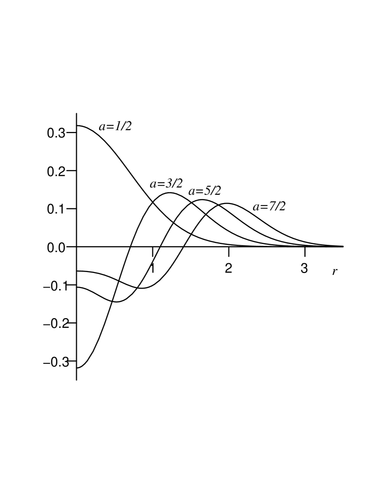
Figure 1: The ground state Wigner function of the one-dimensional parabose oscillator, for values of $a=1/2,\;3/2,\;5/2,\;7/2$ ($m=0,\;1,\;2,\;3$).

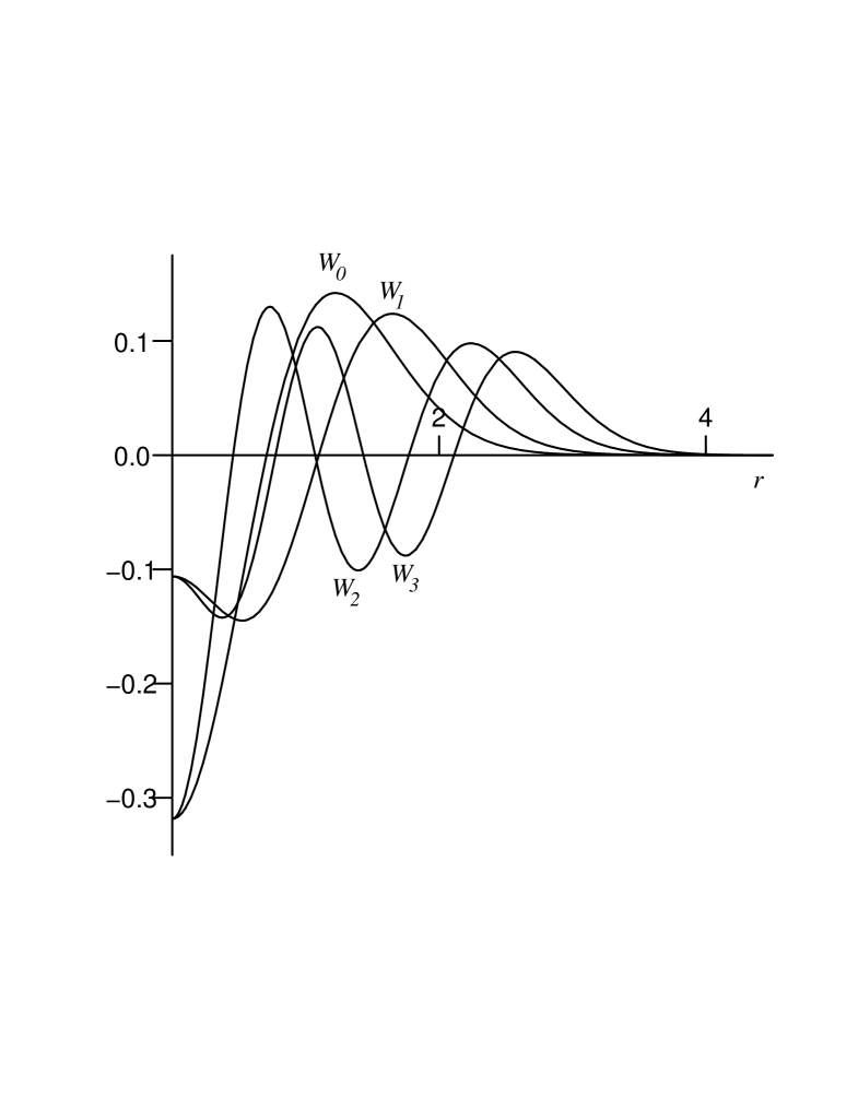
Figure 2: The Wigner function of the stationary states of the one-dimensional parabose oscillator $W_{n}(p,q)$, for fixed value of $a=3/2$ ($m=1$) and $n=0,1,2,3$.

Appendix A

We have to show that

$$\frac{1}{4\pi^{2}}\iint e^{-{(\lambda^{2}+\mu^{2})}/{4}}e^{-i(\lambda p+\mu q)}(\lambda^{2}+\mu^{2})^{k}\,d\lambda d\mu=\frac{1}{\pi}e^{-p^{2}-q^{2}}k!\,4^{k}\,L_{k}(p^{2}+q^{2}),$$ (45)

for $k\in\mathbb{Z}_{+}$ and $p$ and $q$ real. Let us call the left hand side of the expression (45) $I$, and apply the binomial theorem to the factor $(\lambda^{2}+\mu^{2})^{k}$:

$$I=\sum_{j=0}^{k}\binom{k}{j}\left(\frac{1}{2\pi}\int e^{-\lambda^{2}/4-ip\lambda}\lambda^{2j}\,d\lambda\,\right)\left(\frac{1}{2\pi}\int e^{-\mu^{2}/4-iq\mu}\mu^{2k-2j}\,d\mu\right).$$

Each of the two simple integrals above has a known expression in terms of Hermite polynomials [34, 2.3.15.10]:

$$\frac{1}{2\pi}\int e^{-ax^{2}-ibx}x^{2n}\,dx=\frac{(-1)^{n}e^{-b^{2}/4a}}{\sqrt{\pi}2^{2n+1}a^{n}\sqrt{a}}\,H_{2n}(-\frac{b}{2\sqrt{a}}),\quad a>0,\,b\in\mathbb{R}$$

yielding

$$I=\frac{(-1)^{k}}{\pi}e^{-p^{2}-q^{2}}\sum_{j=0}^{k}\binom{k}{j}H_{2j}(-p)H_{2k-2j}(-q).$$

Finally, there is a known summation formula for Hermite polynomials [34, 4.5.2.4]:

$$\sum_{j=0}^{k}\binom{k}{j}H_{2j}(x)H_{2k-2j}(y)=(-1)^{k}k!4^{k}L_{k}(x^{2}+y^{2}).$$

Application of this summation formula immediately yields the desired result (45).

Appendix B

In this Appendix, it is our aim to prove formula (36). We will do so by given formulas for the matrix elements $\langle 2n+2l|\hat{X}^{2k}|2n\rangle$, with $l\in\mathbb{Z}$, which will be seen to reduce to formula (36) when $l=0$. The proof relies on the fact that the formulas given below satisfy the same recurrence and the same boundary conditions as the matrix elements themselves.

With $\hat{X}$ as before, one sees that

$$\hat{X}^{2}=(\alpha^{+})^{2}(\hat{b}^{+})^{2}+\alpha^{+}\alpha^{-}\{\hat{b}^{+},\hat{b}^{-}\}+(\alpha^{-})^{2}(\hat{b}^{-})^{2},$$

and hence one gets, using (14) and (15):

$$\begin{split}\langle 2n+2l|\hat{X}^{2k}|2n\rangle&=\langle 2n+2l|\hat{X}^{2k-2}\hat{X}^{2}|2n\rangle\\ &=(\alpha^{+})^{2}\langle 2n+2l|\hat{X}^{2k-2}(\hat{b}^{+})^{2}|2n\rangle+\alpha^{+}\alpha^{-}\langle 2n+2l|\hat{X}^{2k-2}\{\hat{b}^{+},\hat{b}^{-}\}|2n\rangle\\ &\qquad+(\alpha^{-})^{2}\langle 2n+2l|\hat{X}^{2k-2}(\hat{b}^{-})^{2}|2n\rangle\\ &=2(\alpha^{+})^{2}\sqrt{(n+a)(n+1)}\,\langle 2n+2l|\hat{X}^{2k-2}|2n+2\rangle\\ &\qquad+2\alpha^{+}\alpha^{-}(2n+a)\,\langle 2n+2l|\hat{X}^{2k-2}|2n\rangle\\ &\qquad\qquad+2(\alpha^{-})^{2}\sqrt{n(n+a-1)}\,\langle 2n+2l|\hat{X}^{2k-2}|2n-2\rangle.\end{split}$$

So, if we now denote $\langle 2n+2l|\hat{X}^{2k}|2n\rangle$ as $F_{k,l}(n)$, the recurrence that $F_{k,l}(n)$ satisfies is:

$$\begin{split}F_{k,l}(n)&=2(\alpha^{+})^{2}\sqrt{(n+a)(n+1)}\,F_{k-1,l-1}({n+1})+2\alpha^{+}\alpha^{-}(2n+a)\,F_{k-1,l}(n)\\ &\qquad+2(\alpha^{-})^{2}\sqrt{n(n+a-1)}\,F_{k-1,l+1}({n-1}).\end{split}$$ (46)

From the fact that we are dealing with orthonormal states $|n\rangle$, it follows immediately that

$$F_{0,0}(n)=1,$$ (47)

and also from the actions (14) and (15) it is clear that

$$F_{k,l}(n)=0,\quad\text{if}\ |l|>k.$$ (48)

These two boundary conditions determine the unique solution of the recurrence (46). We will now give explicit formulas that satisfy the boundary conditions (47) and (48), and we will verify that these formulas also satisfy (46). The verification of that last fact will boil down to checking that two polynomials are equal. As a polynomial basis, we will however not choose the classical basis $x^{k}$, but rather we will work with the polynomials $(x)_{k}$.

We now state the formulas,

$$\begin{split}\langle 2n+2l|\hat{X}^{2k}|2n\rangle&=(-1)^{l}2^{k}(\alpha^{+})^{k+l}(\alpha^{-})^{k-l}\sqrt{(n+1)_{l}(n+a)_{l}}\\ &\quad\times\sum_{j=0}^{\min(n,k-l)}\frac{(a+l+j)_{k-l-j}(-n)_{j}(-k)_{l+j}(k+l+1)_{j}}{(l+j)!j!}\end{split}$$ (49)

and

$$\begin{split}\langle 2n-2l|\hat{X}^{2k}|2n\rangle&=(-1)^{l}2^{k}(\alpha^{+})^{k-l}(\alpha^{-})^{k+l}\sqrt{(n-l+1)_{l}(n-l+a)_{l}}\\ &\quad\times\sum_{j=0}^{\min(n-l,k-l)}\frac{(a+l+j)_{k-l-j}(-n+l)_{j}(-k)_{l+j}(k+l+1)_{j}}{(l+j)!j!},\end{split}$$ (50)

where, in both cases, $l\geq 0$. It is immediately clear that formulas (49) and (50) satisfy the boundary conditions (47) and (48). Also, the reduction to (36) for $l=0$ is readily seen.

Since the explicit formulas for the matrix elements are different depending on $l$ being positive or not, checking that (49) and (50) indeed satisfy (46) will involve three cases: $l>0$, $l=0$ and $l<0$. Since all three are very similar, we will only deal with the case $l>0$ here. We will abbreviate the summation in (49) as $S_{k,l}(n)$, then substituting the expression (49) in (46) allows simplification of the powers of $2$ and $\alpha^{\pm}$ as well as the square roots, and leads to the following that needs to be checked:

$$S_{k,l}(n)=-S_{k-1,l-1}({n+1})+(2n+a)S_{k-1,l}(n)-n(n+a-1)S_{k-1,l+1}({n-1}).$$

This is a polynomial identity in the variable $-n$. Let us denote $-n$ as $x$. The coefficients of the polynomials $(x)_{j}$ are immediately clear for the lhs. For the right hand side, one can use the following easy identities:

$$(x-1)_{j}=(x)_{j}-j(x)_{j-1},\quad\text{and}\quad x(x)_{j}=(x)_{j+1}-j(x)_{j}.$$

This allows to extract the coefficient of $(x)_{j}$ in the right hand side. This coefficient is a rational function in the variables $a$, $k$, $j$ and $l$. After clearing the denominator and simplifying the remaining rising factorials, one ends up with a polynomial of a low degree that needs to be identically zero, and that is indeed the case.

So, although the checking is rather tedious, it is at the same time also simple and indeed shows that our formulas for the matrix elements are correct.

We end this appendix by noting that one indeed has:

$$\langle 2n+1+2l|\hat{X}^{k}|2n+1\rangle=\langle 2n+2l|\hat{X}^{k}|2n\rangle|_{a\to a+1}.$$

Indeed, it is easily checked that the recurrence satisfied by $G_{k,l}(n)=\langle 2n+1+2l|\hat{X}^{k}|2n+1\rangle$ is identical to (46) but with $a$ replaced by $a+1$. Also, the boundary conditions for $G$ are identical to (47) and (48) and as these do not involve $a$ the statement is now proved.

Appendix C

In this Appendix, we are briefly going to discuss some aspects of the convergence of the main expressions (32) and (39). The main result is that expressions (32) and (39) converge absolutely when $a>1$ for all $p$ and $q$. In the origin, i.e. $(p,q)=(0,0)$, the condition $a>1$ is also necessary for convergence. For the odd states, we thus have absolute convergence for the expressions derived from (32) and (39) everywhere for $a>0$. The only remaining question is thus what happens for the even states when $(p,q)\neq(0,0)$ in the case $0<a<1$ (and $a\neq 1/2$).

First, let us recall the well known fact that if one has two series of positive terms $\sum_{k}b_{k}$ and $\sum_{k}c_{k}$ such that $b_{k}\leq c_{k}$, then convergence of $\sum_{k}c_{k}$ implies that of $\sum_{k}b_{k}$. Secondly, there are some well known tests for convergence of positive series, one of them is Raabe’s test which can be used if the ratio test fails: let $\sum_{k}b_{k}$ be a series of positive terms and let:

$$\lim_{k\to\infty}k(\frac{b_{k}}{b_{k+1}}-1)=L,$$

one then has that $\sum_{k}b_{k}$ converges if $L>1$ and diverges whenever $L<1$. When $L=1$, the test is inconclusive.

Let us abbreviate $p^{2}+q^{2}$ as $t$. The convergence of (32) then reduces to the convergence of

$$\sum_{k\geq 0}\frac{(1/2-a)_{k}}{(1/2)_{k}}L_{k}(t)=\sum_{k\geq 0}b_{k}.$$ (51)

Next, we are going to use an inequality for the Laguerre polynomials $L_{k}(t)$ which gives an upper bound for $|L_{k}(t)|$ not depending on $k$ [35, 10.18(3)]:

$$|L_{k}(t)|\leq e^{t/2},\ \text{for}\ t\geq 0.$$ (52)

This gives us:

$$|b_{k}|=\left|\frac{(1/2-a)_{k}}{(1/2)_{k}}L_{k}(t)\right|\leq\left|\frac{(1/2-a)_{k}}{(1/2)_{k}}\right|e^{t/2}=c_{k}.$$

The ratio test fails on the series $\sum_{k}c_{k}$, but Raabe’s test gives:

$$\lim_{k\to\infty}k(\frac{c_{k}}{c_{k+1}}-1)=\lim_{k\to\infty}k\left(\frac{|1+2k|}{|1-2a+2k|}-1\right)=\lim_{k\to\infty}k\left(\frac{1+2k}{1-2a+2k}-1\right)=a.$$

So clearly, the series $\sum_{k}c_{k}$ converges if $a>1$, and hence the series (51) is absolutely convergent in that case. Note that the fact that $\sum_{k}c_{k}$ diverges for $a<1$ does not imply anything about the convergence of (32). The issue about the convergence of (32) thus remains open for $0<a\leq 1$. When $t=0$, however, something more can be said:

$$W_{0}(0,0)=\frac{1}{\pi}\sum_{k\geq 0}\frac{(1/2-a)_{k}}{(1/2)_{k}}={}_{2}F_{1}\left(\genfrac{}{}{0.0pt}{}{1/2-a,1}{1/2};1\right).$$

A Gauss hypergeometric series

$${}_{2}F_{1}\left(\genfrac{}{}{0.0pt}{}{a,b}{c};1\right)$$

converges if and only if $\text{Re}(c-a-b)>0$ [22], which in this case amounts to $a>1$.

The convergence behaviour of $W_{1}(p,q)$ is now easy to determine from (34). It is immediately clear that $W_{1}(p,q)$ is absolutely convergent for $a>0$.

For the convergence of (39) we follow the same strategy. First, it is clear that the convergence of

$$\sum_{k}b_{k}=\sum_{k\geq 2j}\frac{k!\,(1/2-a-2n)_{k}}{(1/2)_{k}(k-2j)!}L_{k}(p^{2}+q^{2})$$ (53)

is a sufficient condition for the convergence of (39) since the summation over $j$ is finite. Then, we again use (52), and in this case we get

$$|b_{k}|\leq\left|\frac{k!\,(1/2-a-2n)_{k}}{(1/2)_{k}(k-2j)!}\right|e^{t/2}=c_{k}.$$

Raabe’s test yields in this case that the series $\sum_{k}c_{k}$ is convergent if $a>1+2j-2n$. Since $j\leq n$ (see the summation bounds in (39)), a sufficient (and necessary) condition for this to be true is $a>1$. For $t=0$, use of the convergence of the Gauss hypergeometric series for $z=1$ again yields convergence if and only if $a>1$. Finally, for the functions $W_{2n+1}(p,q)$, we will thus have (absolute) convergence everywhere for $a>0$.

References

- [1] Moshinsky M 1969 The Harmonic Oscillator in Modern Physics: from Atoms to Quarks (New-York: Gordon and Breach)
- [2] Landau L D and Lifshitz E M 1997 Quantum Mechanics: Non-Relativistic Theory (Oxford: Butterworth-Heinemann)
- [3] Wigner E P 1932 Phys. Rev. 40 749
- [4] Ourjoumtsev A, Tualle-Brouri R, Laurat J and Grangier P 2006 Science 312 83
- [5] Leibfried D, Meekhof D M, King B E, Monroe C, Itano W M and Wineland D J 1996 Phys. Rev. Lett. 77 4281
- [6] Smithey D T, Beck M, Raymer M G and Faridani A 1993 Phys. Rev. Lett. 70 1244
- [7] Lvovsky A I, Hansen H, Aichele T, Benson O, Mlynek J and Schiller S 2001 Phys. Rev. Lett. 87 050402
- [8] McMahon P J, Allman B E, Jacobson D L, Arif M, Werner S A and Nugent K A 2003 Phys. Rev. Lett. 91 145502
- [9] Iwata G 1951 Prog. Theor. Phys. 6 524
- [10] Macfarlane A J 1989 J. Phys. A: Math. Gen. 22 4581
- [11] Kagramanov E D, Mir-Kasimov R M and Nagiyev S M 1990 J. Math. Phys. 31 1733
- [12] Bonatsos D and Daskaloyannis C 1999 Prog. Part. Nucl. Phys. 43 537
- [13] Jafarov E I, Lievens S, Nagiyev S M and Van der Jeugt J 2007 J. Phys. A: Math. Theor. 40 5427
- [14] Wigner E P 1950 Phys. Rev. 77 711
- [15] Kamupingene A H, Palev T D and Tsaneva S P 1986 J. Math. Phys. 27 2067
- [16] Connes A 1994 Noncommutative Geometry (San Diego, CA: Academic Press)
- [17] Garay L J 1995 Internat. J. Modern Phys. A 10 145
- [18] Nair V P and Polychronakos A P 2001 Phys. Lett. B 505 267
- [19] Jackiw R 2003 Ann. Henri Poincaré 4S2 S913
- [20] Green H S 1953 Phys. Rev. 90 270
- [21] Ganchev A C and Palev T D 1980 J. Math. Phys. 21 797
- [22] Slater L J 1966 Generalized Hypergeometric Series (Cambridge: Cambridge University Press)
- [23] Koekoek R and Swarttouw R F 1998 The Askey-scheme of hypergeometric orthogonal polynomials and its q-analogue (Delft University of Technology: Report no. 98-17)
- [24] Ohnuki Y and Kamefuchi S 1982 Quantum Field Theory and Parastatistics (New-York: Springer-Verslag)
- [25] Mukunda N, Sudarshan E C G, Sharma J K and Mehta C L 1980 J. Math. Phys. 21 2386
- [26] Tatarskii V I 1983 Sov. Phys. Uspekhi 26 311
- [27] Lee H W 1995 Phys. Rep. 259 147
- [28] Krattenthaler C 1995 J. Symbolic Comput. 20 737
- [29] Paris R B 2005 J. Comput. Appl. Math. 173 379
- [30] Prudnikov A P, Brychkov Y A and Marichev O I 1986 Integrals and Series - vol 2: Special Functions (New-York: Gordon&Breach)
- [31] Calogero F 1969 J. Math. Phys. 10 2191
- [32] Calogero F 1971 J. Math. Phys. 12 419
- [33] Sutherland B 1971 Phys. Rev. A 4 2019
- [34] Prudnikov A P, Brychkov Y A and Marichev O I 1986 Integrals and Series - vol 1: Elementary Functions (New-York: Gordon&Breach)
- [35] Erdélyi A, Magnus W, Oberhettinger F and Tricomi F G 1953 Higher Transcendental Functions Vol 1 (New-York: McGraw-Hill)