Comparing magnetic field extrapolations with measurements of magnetic loops.

We compare magnetic field extrapolations from a photospheric magnetogram with the observationally inferred structure of magnetic loops in a newly developed active region. This is the first time that the reconstructed 3D-topology of the magnetic field is available to test the extrapolations. We compare the observations with potential fields, linear force-free fields and non-linear force-free fields. This comparison reveals that a potential field extrapolation is not suitable for a reconstruction of the magnetic field in this young, developing active region. The inclusion of field-line-parallel electric currents, the so called force-free approach, gives much better results. Furthermore, a non-linear force-free computation reproduces the observations better than the linear force-free approximation, although no free parameters are available in the former case.

1 Introduction

Due to the low plasma $\beta$ the magnetic field is the dominating quantity in the low solar corona. Thus, the 3-D magnetic field structure is of basic importance for physical processes in the solar atmosphere, such as flares, coronal mass ejections and X-ray jets. Direct observations of chromospheric and coronal magnetic fields are difficult, but significant progress has been made within the last few years, e.g. Lee et al. (1999); Lin, Penn, & Tomczyk (2000); Kundu et al. (2001); White (2002); Raouafi et al. (2002); Solanki et al. (2003); Lagg et al. (2004); Lin, Kuhn, & Coulter (2004). Here we compare magnetic loops reconstructed from magnetic field measurements by Solanki et al. (2003) with magnetic fields extrapolated from a photospheric magnetogram. The measured fields allow a much more sensitive test of extrapolations than other observations.

2 Measurements of magnetic fields in the upper chromosphere

The inference of the magnetic vector is based on an inversion technique applied to spectropolarimetric data of the photospheric Si I line at 1082.7 nm and the chromospheric He I 1083 nm triplet. The data were recorded with the Tenerife Infrared Polarimeter mounted on the German Vacuum Tower Telescope (VTT). The spatial resolution of the data was limited by seeing to 1.5″.

The photospheric magnetic vector map was obtained by applying the inversion code SPINOR to the Si I Stokes profiles Frutiger et al. (2000). The He I triplet provided the maps of the chromospheric vector magnetic field. This triplet, which has a complex non-LTE line formation Avrett et al. (1994) but is nearly optically thin Giovanelli & Hall (1977), was analysed by applying the Unno-Rachkowsky solution Unno (1956); Rachkowsky (1967) to describe the individual Zeeman components of each member of the triplet, together with a simple implementation of the Hanle effect based on recent developments. These have convincingly demonstrated that the Hanle effect in forward scattering close to the solar disk center creates measurable linear polarization in spectral lines Trujillo Bueno et al. (2002).

The inclination and azimuthal angle from the chromospheric magnetic field map was used to trace magnetic field lines. We identified field lines as magnetic loops if the following criteria were fulfilled: the magnetic field strength must decrease with height, the inclination and azimuthal angles must not vary strongly from one pixel to the other and the height of the two footpoints must be similar. For a more detailed description of the observations and the analysis technique we refer to Lagg et al. (2004) and Solanki et al. (2003).

We are aware of the assumptions and approximations which enter the magnetic field reconstruction from the polarimetric observations: The Milne-Eddington approach neglects vertical gradients and the simple implementation of the Hanle-effect restricts the reliable determination of the azimuthal angle to regions where the magnetic field is strongly inclined to the line of sight. Furthermore this method neglects the changes in the polarization signal caused by the incomplete Paschen-Back splitting Socas-Navarro, Trujillo Bueno, & Landi Degl’Innocenti (2004). From a preliminary comparison of the obtained H$\alpha$ slit jaw images and the inferred magnetic loops we are confident that the retrieved magnetic field topology is close to the real situation. In the following we use the term ”observed loops” to name the loops inferred under these assumptions and to distinguish them from loops computed with the help of extrapolations from a photospheric magnetogram.

3 Computation of 3D magnetic fields from photospheric magnetic field measurements.

A number of authors have modelled the coronal magnetic field by extrapolating from photospheric magnetic field observations. It is generally assumed that the magnetic pressure in the corona is much higher than the plasma pressure (small plasma $\beta$) and that therefore the magnetic field is nearly force-free. The extrapolation methods based on this assumption include potential field extrapolation (e.g. Semel, 1967), linear force-free field extrapolation (e.g. Chiu and Hilton, 1977; Seehafer, 1978; Seehafer, 1982; Semel, 1988) and nonlinear force-free field extrapolation (e.g. Sakurai, 1981; Roumeliotis, 1996; Amari et al., 1997; Amari et al., 1999; Wheatland et al., 2000; Wiegelmann, 2004). Force-free magnetic fields have to obey the equations

$$(\nabla\times{\bf B})\times{\bf B} = {\bf 0},$$ (1)

$$\nabla\cdot{\bf B} = 0.$$ (2)

which are equivalent to

$$(\nabla\times{\bf B}) = \alpha{\bf B},$$ (3)

$${\bf B}\cdot\nabla\alpha = 0.$$ (4)

In general $\alpha$ is a function of space. Taking this into account corresponds to the non-linear force-free approach. A popular simplification is to choose $\alpha={\rm constant}$ in the entire computational domain, the linear force-free approach. The choice $\alpha=0$ corresponds to current-free potential fields. In this paper we compute potential fields, linear force-free and non-linear force-free fields and compare the result with the magnetic loops reconstructed from the observations.

3.1 Potential and linear force-free fields.

We use the method of Seehafer (1978) for calculating the linear force-free field. The method requires a line-of-sight magnetogram and contains a free scalar parameter $\alpha$, where $\alpha=0$ corresponds to potential fields. The method gives the components of the magnetic field in terms of a Fourier series. The observed magnetogram which covers a rectangular region extending from $0$ to $L_{x}$ in $x$ and $0$ to $L_{y}$ in $y$ is artificially extended onto a rectangular region covering $-L_{x}$ to $L_{x}$ and $-L_{y}$ to $L_{y}$ by taking an antisymmetric mirror image of the original magnetogram in the extended region, i.e. $B_{z}(-x,y)=-B_{z}(x,y)$ and $B_{z}(x,-y)=-B_{z}(x,y)$. The advantage of taking the antisymmetric extension of the original magnetogram is that the extended magnetogram is automatically flux balanced. We use a Fast Fourier Transformation (FFT) scheme to determine the coefficients of the Fourier series. $\alpha$ has the dimension of an inverse length. As a characteristic length scale we choose the harmonic mean $L$ of $L_{x}$ and $L_{y}$. (See Seehafer 1978 for details.)

3.2 Non-linear force-free fields.

We solve Eqs. (1) and (2) by means of an optimization principle (Wheatland et al. 2000, Wiegelmann 2004):

$$L=\int_{V}w(x,y,z)\,\left[B^{-2}\,|(\nabla\times{\bf B})\times{\bf B}|^{2}+|\nabla\cdot{\bf B}|^{2}\right]\,d^{3}x,$$ (5)

where $w(x,y,z)$ is a weighting function. It is obvious that (for $w>0$) the force-free Eqs. (1-2) are fulfilled when L equals zero. We compute the magnetic field in a box with $nx=95$, $ny=68$ and $nz=40$ points. The numerical method works as follows. As an initial configuration we compute a potential magnetic field in the whole box with the help of the Seehafer (1978) method. As the next step we use photospheric vector magnetic field data to prescribe the bottom boundary (photosphere) of the computational box. On the lateral and top boundaries the field is chosen from the potential field above. We iterate for the magnetic field inside the computational box by minimizing Eq. (5). The weighting function $w$ equals 1 everywhere in the computational box except in a boundary layer of $10$ points towards the lateral and top boundary of the computational box, where $w$ decreases smoothly to 0 with a cosine function. The boundary layer diminishes the influence of the lateral and top boundary conditions onto the magnetic field in the box. (See Wiegelmann 2004 for details.)

4 Results

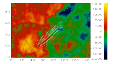
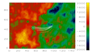
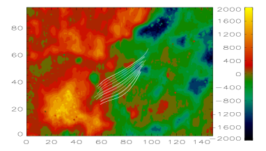
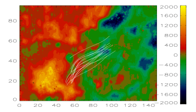
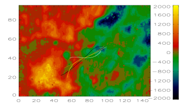
Figure 1: Observed and extrapolated fields. The left panels show the field lines in 3D and the right panels projections on the photosphere. The photospheric LOS field is represented by colour-coding. Top panels: Original observed loops. We show 14 out of a total of 39 loops studied here. Second row: potential field extrapolation. Third row: linear force-free field extrapolation with $\alpha\cdot L=3.0$. Fourth: non-linear force-free field extrapolation. The fifth row shows one loop (Black: original, white: potential field, orange: linear force-free field with $\alpha\cdot L=3.0$, yellow: non-linear force-free field.)

To compare the reconstructed magnetic field with the observed magnetic loops we compute magnetic field lines from the reconstructed fields using a fourth order Runge-Kutta field-line tracer. The field-line tracer starts the integration at any arbitrary point in space and traces the magnetic field in the $+B$ and $-B$ direction until the photosphere is reached in both directions. As a measure of how well the magnetic field lines and the observed loops agree, we compute the spatial distance of the two curves in 3D integrated along the whole loop length $l$ from $\tau=0$ to $\tau=l$. As a result we get a dimensionless number $C=\frac{1}{l^{2}}\int_{0}^{l}\sqrt{\left({\bf r_{\rm obs}}(\tau)-{\bf r_{\rm extrapol}}(\tau)\right)^{2}}d\tau$, where $\tau$ is the geometrical length measured along the loop and $C=0$ if both curves coincide. This comparison method has been previously used by Wiegelmann & Neukirch (2002) to compare magnetic field lines with stereoscopically observed loops.

We start the field line integration at 20 points each chosen to lie along an observed field line ${\bf r_{\rm obs}}(\tau)$ and compute 20 corresponding field lines. We compare the shapes of these computed field lines (loops) with the observed field line and compute the quantitative measure $C$. The lowest value of $C$ corresponds to the optimal computed magnetic field line. For potential fields and non-linear force-free fields the choice of the starting point is the only free parameter and finding the optimal field line is a one-dimensional minimization problem. Linear force-free fields have the free parameter $\alpha$ and computing the optimal linear force-free field line is a two-dimensional minimization problem with respect to $\alpha$ and the integration starting point.

Fourteen representative loops are shown in Fig. 1 with observed, potential, linear and non-linear force-free loops being plotted from top to bottom. This figure shows, that force-free extrapolations are superior to potential fields, with non-linear force-free being apparently the closest to the observations. A more quantitative measure is provided by the $C$ values, which are given for all 39 observed loops in Fig. 2 and Table 1. The lower the value of $C$ the better the reconstructed loops agree with the observed loops. A value of $C\leq 0.35$ seems to be acceptable.

We find that the simplest magnetic field model, potential fields (second row in Fig. 1, Fig. 2 a), provides no agreement with any observed loop (top row in Fig. 1) within the $C\leq 0.35$ limit.

The inclusion of electric currents, in lowest order with the linear force-free approximation (Fig. 2 b) provides better results, and for $35\%$ of the observed loops we get satisfying agreement with the observations. One has to keep in mind, however, that a consistent linear force-free reconstruction requires a unique value of $\alpha$ in the entire considered volume. Most of the loops have an optimum value of $\alpha L$ in the range $3-4$ and the quality criterion $C$ only changes slightly within this range, so that a unique value of $\alpha$ in this range does not give significantly worse results than the optimal value of $\alpha$. The linear force-free fields in Fig. 1, third row have been computed with $\alpha L=3$.

The most involved model used here, the non-linear force-free approach (fourth row in Fig. 1 and Fig. 2 c), gives even better results than the linear force free approach. We get a suitable agreement with the observed loops for $64\%$ of the loops within the $C\leq 0.35$ limit. Let us remark that all observed loops which cannot be reconstructed with this model have at least one foot point close to the boundary of the available vector magnetic field data. (see Fig. 3).

Figure 2: Correspondence of extrapolated loops and measured loops for all $39$ observed loops. The panels (a)-(c) show distributions over $C$ for potential, linear and non-linear force-free fields, respectively. Panel (d) shows the value for all loops. The rhombi correspond to a potential field reconstruction, the stars to the optimal linear force-free reconstruction and the triangles to a non-linear force-free reconstruction. (See also Table 1 for the $C$-values of the individual loops.)

Table 1: The first column corresponds to an arbitrary loop number of the observed loops, the second column compares the measured loops with a potential field extrapolation. Cols. 3 and 4 compare the observed loops with linear force-free fields and $\alpha L=3$ and $\alpha L=4$, respectively. The fifth column contains the optimal linear force-free parameter $\alpha L$ and the sixth column the comparison with the observed loops for this optimal value. In the last column we compare the observations with non-linear force-free reconstructed magnetic loops.

Nr	$C_{\rm pot}$	$C_{\rm lin}$	$C_{\rm lin}$	$\alpha_{\rm opt}$	$C_{\rm lin}$	$C_{\rm nonlin}$
		$\alpha L=3$	$\alpha L=4$		$\alpha_{\rm opt}$
0	$1.69$	$1.40$	$1.06$	$4.2$	$1.04$	$1.60$
1	$1.13$	$0.83$	$0.86$	$2.6$	$0.79$	$0.86$
2	$0.48$	$0.30$	$0.28$	$3.5$	$0.27$	$0.15$
3	$0.57$	$0.34$	$0.31$	$3.7$	$0.30$	$0.14$
4	$0.75$	$0.64$	$0.65$	$3.2$	$0.63$	$0.65$
5	$0.80$	$0.52$	$0.45$	$3.8$	$0.45$	$0.19$
6	$0.69$	$0.37$	$0.31$	$4.1$	$0.30$	$0.17$
7	$0.90$	$0.56$	$0.43$	$4.3$	$0.40$	$0.12$
8	$0.58$	$0.35$	$0.30$	$3.8$	$0.29$	$0.14$
9	$1.90$	$1.57$	$1.39$	$4.2$	$1.05$	$1.38$
10	$0.68$	$0.44$	$0.51$	$3.0$	$0.44$	$0.59$
11	$0.43$	$0.26$	$0.29$	$2.9$	$0.25$	$0.25$
12	$0.98$	$0.56$	$0.73$	$3.5$	$0.52$	$1.01$
13	$0.89$	$0.86$	$0.87$	$3.5$	$0.85$	$0.95$
14	$1.12$	$0.66$	$0.53$	$3.7$	$0.52$	$0.26$
15	$1.05$	$0.63$	$0.49$	$4.0$	$0.49$	$0.20$
16	$0.66$	$0.35$	$0.29$	$4.1$	$0.29$	$0.15$
17	$0.43$	$0.27$	$0.28$	$3.0$	$0.27$	$0.21$
18	$0.41$	$0.26$	$0.26$	$3.3$	$0.25$	$0.16$
19	$0.48$	$0.30$	$0.30$	$3.3$	$0.28$	$0.16$
20	$0.67$	$0.35$	$0.31$	$4.4$	$0.29$	$0.19$
21	$0.49$	$0.34$	$0.30$	$3.6$	$0.29$	$0.20$
22	$0.74$	$0.53$	$0.42$	$4.4$	$0.42$	$0.18$
23	$0.45$	$0.31$	$0.28$	$3.3$	$0.27$	$0.34$
24	$0.48$	$0.35$	$0.31$	$3.4$	$0.31$	$0.29$
25	$0.52$	$0.38$	$0.36$	$4.2$	$0.34$	$0.20$
26	$0.52$	$0.38$	$0.34$	$4.0$	$0.34$	$0.26$
27	$0.58$	$0.40$	$0.48$	$2.6$	$0.37$	$0.24$
28	$0.66$	$0.45$	$0.57$	$2.5$	$0.39$	$0.23$
29	$0.81$	$0.61$	$0.84$	$2.8$	$0.60$	$0.82$
30	$1.01$	$0.68$	$1.25$	$3.2$	$0.67$	$1.40$
31	$1.44$	$0.98$	$0.80$	$3.6$	$0.63$	$2.73$
32	$1.33$	$0.70$	$0.79$	$3.0$	$0.70$	$0.72$
33	$1.30$	$0.71$	$0.71$	$3.2$	$0.64$	$0.53$
34	$1.25$	$0.72$	$0.60$	$3.4$	$0.57$	$0.34$
35	$1.02$	$0.64$	$0.49$	$4.0$	$0.49$	$0.20$
36	$1.94$	$1.66$	$1.32$	$4.2$	$1.30$	$1.57$
37	$0.79$	$0.48$	$0.37$	$4.0$	$0.37$	$0.28$
38	$1.11$	$1.27$	$1.30$	$-0.2$	$1.11$	$1.50$

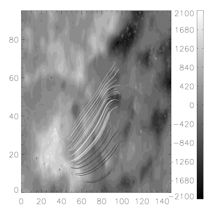
Figure 3: A projection of all observed loops on the photosphere. We can reconstruct the white loops with the help of a non-linear force-free field extrapolation with an accuracy of $C<0.35$. The black loops cannot be reconstructed with adequate accuracy.

5 Conclusions

We have compared the observationally inferred structure of magnetic loops in the upper chromosphere with magnetic fields extrapolated from photospheric measurements. We find that the simplest model, potential fields, is not sufficient to reproduce the observations. The inclusion of field line parallel currents, the so called force-free approach, gives much better results. Among force-free models, a linear one gives less accurate results than the non-linear force-free extrapolation.

We find that the observed and extrapolated loops agree quite well for almost $2/3$ of the loops, while the remaining $1/3$ might suffer from the limited field of view of the available vector magnetogram.

The investigated active region is quite young. With a vertical upflow speed of $v=1.5{{}^{+}_{-}}0.5{\rm km/s}$ at the loop apex and a maximum loop height of $10{\rm Mm}$ we can estimate the time elapsed since the loop tops first emerged as $2{\rm h}{{}^{+}_{-}}40{\rm min}$ assuming a constant rise speed. A horizontal shear flow of $1{\rm km/s}$ on the photosphere would give a shear of $7.2{\rm Mm}$. This value is comparable to the difference of the footpoint locations between potential field loops and observed loops. It is therefore not clear, whether the electric current has been caused by shear flow motion or if the magnetic loops already contain the current during their emergence. The rise of the loops may also explain some of the discrepancy between observed and extrapolated loops, since the loops may change somewhat during the time needed for the instrument to scan the region.