Transverse coherence properties of X-ray beams in third-generation synchrotron radiation sources

Abstract

This article describes a complete theory of spatial coherence for undulator radiation sources. Current estimations of coherence properties often assume that undulator sources are quasi-homogeneous, like thermal sources, and rely on the application of the van Cittert-Zernike theorem for calculating the degree of transverse coherence. Such assumption is not adequate when treating third generation light sources, because the vertical (geometrical) emittance of the electron beam is comparable or even much smaller than the radiation wavelength in a very wide spectral interval that spans over four orders of magnitude (from $0.1\mathrm{\AA}$ up to $10^{3}\mathrm{\AA}$). Sometimes, the so-called Gaussian-Schell model, that is widely used in statistical optics in the description of partially-coherent sources, is applied as an alternative to the quasi-homogeneous model. However, as we will demonstrate, this model fails to properly describe coherent properties of X-ray beams from non-homogeneous undulator sources. As a result, a more rigorous analysis is required. We propose a technique, based on statistical optics and Fourier optics, to explicitly calculate the cross-spectral density of an undulator source in the most general case, at any position after the undulator. Our theory, that makes consistent use of dimensionless analysis, allows relatively easy treatment and physical understanding of many asymptotes of the parameter space, together with their region of applicability. Particular emphasis is given to the asymptotic situation when the horizontal emittance is much larger than the radiation wavelength, and the vertical emittance is arbitrary. This case is practically relevant for third generation synchrotron radiation sources.

1 Introduction

In recent years, continuous evolution of synchrotron radiation (SR) sources has resulted in a dramatic increase of brilliance with respect to older designs. Among the most exciting properties of third generation facilities of today is a high flux of coherent X-rays EDGA . The availability of intense coherent X-ray beams has triggered the development of a number of new experimental techniques based on coherence properties of light such as scattering of coherent X-ray radiation, X-ray photon correlation spectroscopy and phase contrast imaging. The interested reader may find an extensive reference list to these applications in PETR .

Characterization of transverse coherence properties of SR at a specimen position is fundamental for properly planning, conducting and analyzing experiments involving above-mentioned techniques. These objectives can only be met once coherence properties of undulator sources are characterized and then propagated along the photon beamline up to the specimen.

This paper is mainly dedicated to a description of transverse coherence properties of SR sources. Therefore, it constitutes the first step for tracking coherence properties through optical elements, which can be only done when the source is quantitatively described. Solution of the problem of evolution of radiation properties in free-space is also given. This can be used to characterize radiation at the specimen position when there are no optical elements between the source and the specimen.

Since SR is a random process, the description of transverse coherence properties of the source and its evolution should be treated in terms of probabilistic statements. Statistical optics GOOD , MAND , NEIL presents most convenient tools to deal with fluctuating electromagnetic fields. However, it was mainly developed in connection with polarized thermal light that is characterized by quite specific properties. Besides obeying Gaussian statistics, polarized thermal light has two other specific characteristics allowing for major simplifications of the theory: stationarity and homogeneity (i.e. perfect incoherence) of the source GOOD , MAND .

As we will see, SR obeys Gaussian statistics, but stationarity and homogeneity do not belong to SR fields. Thus, although the language of statistical optics must be used to describe SR sources, one should avoid a-priori introduction of an incorrect model. In contrast to this, up to now it has been a widespread practice to assume that undulator sources are perfectly incoherent (homogeneous) and to draw conclusions about transverse coherence properties of undulator light based on these assumptions PETR .

In particular, in the case of thermal light, transverse coherence properties of the radiation can be found with the help of the well-known van Citter-Zernike (VCZ) theorem. However, for third generation light sources either planned or in operation, the horizontal electron beam (geometrical) emittance is of order of $1\div 3$ nm while the vertical emittance is bound to the horizontal through a coupling factor $\zeta\sim 10^{-2}$, corresponding to vertical emittances of order $0.1\div 0.3~{}\mathrm{\AA}$. As we will show, these facts imply that the VCZ theorem cannot be applied in the vertical direction, aside for the hard X-ray limit at wavelengths shorter than $0.1~{}\mathrm{\AA}$. Similar remarks hold for future sources, like Energy Recovery Linac (ERL)-based spontaneous radiators. ERL technology is expected to constitute the natural evolution of today SR sources and to provide nearly fully diffraction-limited sources in the $1\AA$-range, capable of three order of magnitudes larger coherent flux compared to third generation light sources EDGA . Horizontal and vertical emittance will be of order of $0.3\AA$, which rules out the applicability of the VCZ theorem.

The need for characterization of partially coherent undulator sources is emphasized very clearly in reference HOWE . However, studying spatial-coherence properties of undulator sources is not a trivial task. Difficulties arise when one tries to simultaneously include the effect of intrinsic divergence of undulator radiation, and of electron beam size and divergence.

An attempt to find the region of applicability of the VCZ theorem for third generation light sources is reported in TAKA . Authors of TAKA conclude that the VCZ theorem can only be applied when SR sources are close to the diffraction limit. We will see that the VCZ theorem can only be applied in the opposite case.

A model to describe partially-coherent sources, the Gaussian-Schell model, is widely used in statistical optics. Its application to SR is described in COI1 , COI2 , COI3 . The Gaussian-Schell model includes non-homogeneous sources, because the typical transverse dimension of the source can be comparable or smaller than the transverse coherence length. While COI1 , COI2 , COI3 are of general theoretical interest, they do not provide a satisfactory approximation of third generation SR sources. In fact, as we will see, undulator radiation has very specific properties that cannot be described in terms of Gaussian-Schell model.

The first treatment of transverse coherence properties from SR sources accounting for the specific nature of undulator radiation and anticipating operation of third generation SR facilities is given, in terms of Wigner distribution, in KIM2 , KIM3 . References KIM2 , KIM3 present the most general algorithm for calculating properties of undulator radiation sources.

In the present paper we base our theory on the characterization of the cross-spectral density of the system. The cross-spectral density is merely the statistical correlation function of the radiation field at two different positions on the observation plane at a given frequency. It is equivalent to the Wigner distribution, the two quantities being related by Fourier transformation. Based on cross-spectral density we developed a comprehensive theory of third generation SR sources in the space-frequency domain, where we exploited the presence of small or large parameters intrinsic in the description of the system. First, we took advantage of the particular but important situation of perfect resonance, when the field from the undulator source can be presented in terms of analytical functions. Second, we exploited the practical case of a Gaussian electron beam, allowing further analytical simplifications. Third, we took advantage of the large horizontal emittance (compared with the radiation wavelength) of the electron beam, allowing separate treatments of horizontal and vertical directions. Finally, we studied asymptotic cases of our theory for third generation light sources with their region of applicability. In particular, we considered both asymptotes of a small and a large vertical emittance compared with the radiation wavelength, finding surprising results. In the case of a small vertical emittance (smaller than the radiation wavelength) we found that the radiation is not diffraction limited in the vertical direction, an effect that can be ascribed to the influence of the large horizontal emittance on the vertical coherence properties of radiation. In the case of a large vertical emittance we described the quasi-homogeneous source in terms of a non-Gaussian model, which has higher accuracy and wider region of applicability with respect to a simpler Gaussian model. In fact, the non-Gaussian model proposed in our work accounts for diffraction effects. Nonetheless, in order to solve the propagation problem in free-space, a geometrical optics approach can still be used.

We organize our work as follows. First, a general algorithm for the calculation of the field correlation function of an undulator source is given in Section 2. Such algorithm is not limited to the description of third generation light sources, but can also be applied, for example, to ERL sources. In Section 3 we specialize our treatment to third generation light sources exploiting a large horizontal emittance compared to the radiation wavelength, and studying the asymptotic limit for a small vertical emittance of the electron beam. In the following Section 4 we consider the particular case of quasi-homogeneous undulator sources, and discuss the applicability range of the van VCZ theorem. Finally, in Section 5 we come to conclusions.

2 Cross-spectral density of an undulator source

2.1 Thermal light and Synchrotron Radiation: some concepts and definitions

The great majority of optical sources emits thermal light. Such is the case of the sun and the other stars, as well as of incandescent lamps. This kind of radiation consists of a large number of independent contributions (radiating atoms) and is characterized by random amplitudes and phases in space and time. Its electromagnetic field can be conveniently described in terms of statistical optics that has been intensively developed during the last few decades GOOD , MAND .

Figure 1: Light intensity from an incandescent lamp driven by a constant electric current. A statistically stationary wave has an average that does not vary with time.

Consider the light emitted by a thermal source passing through a polarization analyzer, as in Fig. 1. Properties of polarized thermal light are well-known in statistical optics, and are referred to as properties of completely chaotic, polarized light GOOD , MAND . Thermal light is a statistical random process and statements about such process are probabilistic statements. Statistical processes are handled using the concept of statistical ensemble, drawn from statistical mechanics, and statistical averages are performed over an ensemble, or many realizations, or outcomes of the statistical process under study. Polarized thermal sources obey a very particular kind of random process in that it is Gaussian and stationary. Moreover, they are homogeneous.

The properties of Gaussian random processes are well-known in statistical optics. For instance, the real and imaginary part of the complex amplitudes of the electric field from a polarized thermal source have Gaussian distribution, while the instantaneous radiation power fluctuates in accordance with the negative exponential distribution. It can be shown GOOD that a linearly filtered Gaussian process is also a Gaussian random process. As a result, the presence of a monochromator and a spatial filter as in the system depicted in Fig. 1 do not change the statistics of the signal. Finally, higher order field correlation functions can be found in terms of the second order correlation. This dramatically simplifies the description of the random process.

Stationarity is a subtle concept. There are different kinds of stationarity. However, for Gaussian processes different kinds of stationarity coincide GOOD , MAND . In this case, stationarity means that all ensemble averages are independent of time. It follows that a necessary condition for a certain process to be stationary is that the signal last forever. Yet, if a signal lasts much longer than the short-scale duration of the field fluctuations (its coherence time $\tau_{c}$) and it is observed for a time much shorter than its duration $\sigma_{T}$, but much longer than $\tau_{c}$ it can be reasonably considered as everlasting and it has a chance to be stationary as well, as in the case of thermal light.

Finally, thermal sources are homogeneous. The field is correlated on the transverse direction over the possible minimal distance, which is of order of a wavelength. This means that the radiation intensity at the source remains practically unvaried on the scale of a correlation length. One can say, equivalently, that the source is homogeneous. Homogeneity is the equivalent, in the transverse direction, of stationarity and implies a constant ensemble-averaged intensity along the transverse direction.

Consider now a SR source, as depicted in Fig. 2. Like thermal light, also SR is a random process. In fact, relativistic electrons in a storage ring emit SR passing through bending magnets or undulators. The electron beam shot noise causes fluctuations of the beam density which are random in time and space from bunch to bunch. As a result, the radiation produced has random amplitudes and phases. Moreover, in Section 2.2 we will demonstrate that SR fields obey Gaussian statistics. Statistical properties satisfied by single-electron contributions (elementary phasors) to the total SR field are weaker than those satisfied by single-atom contributions in thermal sources. Thus, the demonstration that thermal light obeys Gaussian statistics cannot be directly applied to the SR case, and some condition should be formulated on the parameter space to define the region where SR is indeed a Gaussian random process. We will show this fact with the help of Appendix A of OURU .

In contrast with thermal light, SR is intrinsically non-stationary, because it presents a time-varying ensemble-averaged intensity on the temporal scale of the duration of the X-ray pulse generated by a single electron bunch. For this reason, in what follows the averaging brackets $\langle...\rangle$ will always indicate the ensemble average over bunches (and not a time average).

Figure 2: The intensity of an X-ray beam from a SR source. A statistically non-stationary wave has a time-varying intensity averaged over an ensemble of bunches.

Finally, SR sources are not completely incoherent, or homogeneous. In fact, there is a close connection between the state of coherence of the source and the angular distribution of the radiant intensity. A thermal source that is correlated over the minimal possible distance (which is of order of the wavelength) is characterized by a radiant intensity distributed over a solid angle of order $2\pi$. This is not the case of SR light, that is confined within a narrow cone in the forward direction. The high directionality of SR rules out the possibility of description in terms of thermal light. As we will see, depending on the situation, SR may or may not be described by a quasi-homogeneous model, where sources are only locally coherent over a distance of many wavelengths but the linear dimension of the source is much larger than the correlation distance.

In spite of differences with respect to the simpler case of thermal light, SR fields can be described in terms of statistical optics. However, statistical optics was developed in relation with thermal light emission. Major assumptions typical of this kind of radiation like, for example, stationarity, are retained in textbooks GOOD , MAND . Thus, usual statistical optics treatment must be modified in order to deal with SR problems. We will reduce the problem of characterization of transverse coherence properties of undulator sources in the space-frequency domain to the calculation of the correlation of the field produced by a single electron with itself. This correlation is known as cross-spectral density. The non-stationarity of the process imposes some (practically non restrictive) condition on the parameter space region where a treatment based on cross-spectral density can be applied to SR phenomena. Such condition involves the length of the electron bunch, the number of undulator periods and the radiation wavelength. Given the fact that the electron bunch length can vary from about $10$ ps for third generation SR sources to about $100$ fs for ERL sources, understanding of the region of applicability this condition is a-priori not obvious. All these subjects will be treated in the next Section 2.2.

2.2 Second-order correlations in space-frequency domain

In SR experiments with third generation light sources, detectors are limited to about $100$ ps time resolution. Therefore, they cannot resolve a single X-ray pulse in time domain, whose duration is about $30$ ps. They work, instead, by counting the number of photons at a certain frequency over an integration time longer than the pulse. It is therefore quite natural to consider signals in the frequency domain. With this in mind, let ${\bar{E}}_{b}(z,\vec{r},\omega)$ be a fixed polarization component of the Fourier transform of the electric field at location $(z,\vec{r})$, in some cartesian coordinate system, and frequency $\omega$ by a given collection of electromagnetic sources. We will often name it, slightly improperly, ”the field”. Subscript ”b” indicates that the field is generated by the entire bunch. ${\bar{E}}_{b}(z,\vec{r},\omega)$ is linked to the time domain field ${{E}}_{b}(z,\vec{r},t)$ through the Fourier transform

$$\bar{{E}}_{b}(\omega)=\int_{-\infty}^{\infty}dt{{E}}_{b}(t)\exp(i\omega t)~{},~{}~{}~{}~{}~{}{{E}}_{b}(t)=\frac{1}{2\pi}\int_{-\infty}^{\infty}d\omega\bar{{E}}_{b}(\omega)\exp(-i\omega t)~{}.$$ (1)

We will be interested in the case of an ultra relativistic electron beam going through a certain magnetic system, an undulator in particular. In this case $z$ is the observation distance along the optical axis of the undulator and $\vec{r}$ fixes the transverse position of the observer. The contribution of the $k$-th electron to the field depends on the transverse offset $\vec{l}_{k}$ and deflection angles $\vec{\eta}_{k}$ that the electron has at some reference point on the optical axis $z$, e.g. the center of the undulator. Moreover, the arrival time $t_{k}$ at the center of the undulator has the effect of multiplying the field by a phase factor $\exp{(i\omega t_{k})}$, i.e. the time-domain electric field is retarded by a time $t_{k}$. At this point we do not need to explicitly specify the dependence on offset and deflection. The total field can be written as

$${\bar{E}}_{b}\left(z,\vec{r},\omega\right)=\sum_{k=1}^{N_{e}}\bar{E}\left(\vec{\eta}_{k},\vec{l}_{k},z,\vec{r},\omega\right)\exp{(i\omega t_{k})}~{},$$ (2)

where $\vec{\eta}_{k},\vec{l}_{k}$ and $t_{k}$ are random variables and $N_{e}$ is the number of electrons in the bunch. Note that $\bar{E}$ in Eq. (2) is a complex quantity, that can be written as $\bar{E}=\mid\bar{E}_{k}\mid\exp(i\phi_{k})$. It follows that the SR field pulse at fixed frequency and position is a sum of a many phasors, one for each electron, of the form $\bar{E}\exp{(i\omega t_{k})}=\mid\bar{E}_{k}\mid\exp(i\phi_{k}+i\omega t_{k})$.

Elementary phasors composing the sum obey three statistical properties, that are satisfied in SR problems of interest. First, random variables $t_{k}$ are statistically independent of each other, and of variables $\vec{\eta}_{k}$ and $\vec{l}_{k}$. Second, random variables $\mid\bar{E}_{k}\mid$ (at fixed frequency $\omega$), are identically distributed for all values of $k$, with a finite mean $\langle\mid\bar{E}_{k}\mid\rangle$ and a finite second moment $\langle\mid\bar{E}_{k}\mid^{2}\rangle$. These two assumptions follows from the properties of shot noise in a storage ring, which is a fundamental effect related with quantum fluctuations. Third, we assume that the electron bunch duration $\sigma_{T}$ is large enough so that $\omega\sigma_{T}\gg 1$: under this assumption, phases $\omega t_{k}$ can be regarded as uniformly distributed on the interval $(0,2\pi)$. The assumption $\omega\sigma_{T}\gg 1$ exploits the first large parameter of our theory, and is justified by the fact that $\omega$ is the undulator resonant frequency, which is high enough, in practical cases of interest, to guarantee that $\omega\sigma_{T}\gg 1$ for any realistic choice of $\sigma_{T}$. Based on the three previously discussed properties, and with the help of the central limit theorem, it can be demonstrated that the real and the imaginary part of $\bar{E}_{b}$ are distributed in accordance to a Gaussian law.

As a result, SR is a non-stationary Gaussian random process.

Because of this, higher-order correlation functions can be expressed in terms of second-order correlation functions with the help of the moment theorem GOOD . As a result, the knowledge of the second-order field correlation function in frequency domain, $\Gamma_{\omega}$, is all we need to completely characterize the signal from a statistical viewpoint. The following definition holds:

$$\Gamma_{\omega}\left(z,\vec{r}_{{}1},\vec{r}_{{}2},\omega_{1},\omega_{2}\right)=\left<{\bar{E}}_{b}\left(z,\vec{r}_{{}1},\omega_{1}\right){\bar{E}}^{*}_{b}\left(z,\vec{r}_{{}2},\omega_{2}\right)\right>~{},$$ (3)

where brackets $<...>$ indicate ensemble average over electron bunches. For any given function $w\left(\vec{\eta}_{k},\vec{l}_{k},t_{k}\right)$, the ensemble average is defined as

$$\left<w\left(\vec{\eta}_{k},\vec{l}_{k},t_{k}\right)\right>=\int d\vec{\eta}_{k}\int d\vec{l}_{k}\int_{-\infty}^{\infty}dt_{k}w\left(\vec{\eta}_{k},\vec{l}_{k},t_{k}\right)P\left(\vec{\eta}_{k},\vec{l}_{k},t_{k}\right)~{},$$ (4)

where integrals in $d\vec{l}_{k}$ and $d\vec{\eta}_{k}$ span over all offsets and deflections, and $P=P(\vec{\eta}_{k},\vec{l}_{k},t_{k})$ indicates the probability density distribution in the joint random variables $\vec{\eta}_{k}$, $\vec{l}_{k}$, and $t_{k}$. Note that, since all electrons have the same probability of arrival around a given offset, deflection, and time, $P$ is independent of $k$. Moreover, already discussed independence of $t_{k}$ from $\vec{l}_{k}$ and $\vec{\eta}_{k}$ allows to write $P$ as

$$P\left(\vec{\eta}_{k},\vec{l}_{k},t_{k}\right)=f_{\bot}\left(\vec{l}_{k},\vec{\eta}_{k}\right)f(t_{k})~{}.$$ (5)

Here $f$ is the longitudinal bunch profile of the electron beam, while $f_{\bot}$ is the transverse phase-space distribution.

Substituting Eq. (2) in Eq. (3) one has

$$\Gamma_{\omega}=\left<\sum_{m,n=1}^{N_{e}}\bar{E}\left(\vec{\eta}_{m},\vec{l}_{m},z,\vec{r}_{{}1},\omega_{1}\right)\bar{E}^{*}\left(\vec{\eta}_{n},\vec{l}_{n},z,\vec{r}_{{}2},\omega_{2}\right)\exp{[i(\omega_{1}t_{m}-\omega_{2}t_{n})]}\right>.$$ (6)

(7)

Expansion of Eq. (7) gives

$$\Gamma_{\omega}=\sum_{m=1}^{N_{e}}\left\langle\bar{E}\left(\vec{\eta}_{m},\vec{l}_{m},z,\vec{r}_{{}1},\omega_{1}\right)\bar{E}^{*}\left(\vec{\eta}_{m},\vec{l}_{m},z,\vec{r}_{{}2},\omega_{2}\right)\exp{[i(\omega_{1}-\omega_{2})t_{m}]}\right\rangle$$ (8)

$$+\sum_{m\neq n}\left\langle\bar{E}\left(\vec{\eta}_{m},\vec{l}_{m},z,\vec{r}_{{}1},\omega_{1}\right)\exp{(i\omega_{1}t_{m})}\right\rangle\left\langle\bar{E}^{*}\left(\vec{\eta}_{n},\vec{l}_{n},z,\vec{r}_{{}2},\omega_{2}\right)\exp{(-i\omega_{2}t_{n})}\right\rangle.$$ (9)

(10)

With the help of Eq. (4) and Eq. (5), the ensemble average $\langle\exp{(i\omega t_{k})}\rangle$ can be written as the Fourier transform of the longitudinal bunch profile function $f$, that is

$$\left\langle\exp{(i\omega t_{k})}\right\rangle=\int_{-\infty}^{\infty}dt_{k}f(t_{k})\exp(i\omega t_{k})\equiv\bar{f}(\omega)~{}.$$ (11)

Using Eq. (11), Eq. (10) can be written as

$$\Gamma_{\omega} =\sum_{m=1}^{N_{e}}\bar{f}(\omega_{1}-\omega_{2})\left\langle\bar{E}\left(\vec{\eta}_{m},\vec{l}_{m},z,\vec{r}_{{}1},\omega_{1}\right)\bar{E}^{*}\left(\vec{\eta}_{m},\vec{l}_{m},z,\vec{r}_{{}2},\omega_{2}\right)\right\rangle$$ (13)

$$+\sum_{m\neq n}\bar{f}(\omega_{1})\bar{f}(-\omega_{2})\left\langle\bar{E}\left(\vec{\eta}_{m},\vec{l}_{m},z,\vec{r}_{{}1},\omega_{1}\right)\right\rangle\left\langle\bar{E}^{*}\left(\vec{\eta}_{n},\vec{l}_{n},z,\vec{r}_{{}2},\omega_{2}\right)\right\rangle~{},$$

where $\bar{f}^{*}(\omega_{2})=\bar{f}(-\omega_{2})$ because ${f}$ is a real function. When the radiation wavelengths of interest are much shorter than the bunch length we can safely neglect the second term on the right hand side of Eq. (13) since the form factor product $\bar{f}(\omega_{1})\bar{f}(-\omega_{2})$ goes rapidly to zero for frequencies larger than the characteristic frequency associated with the bunch length: think for instance, at a centimeter long bunch compared with radiation in the Angstrom wavelength range. Therefore we write

$$\Gamma_{\omega} =\sum_{m=1}^{N_{e}}\bar{f}(\omega_{1}-\omega_{2})\left\langle\bar{E}\left(\vec{\eta}_{m},\vec{l}_{m},z,\vec{r}_{{}1},\omega_{1}\right)\bar{E}^{*}\left(\vec{\eta}_{m},\vec{l}_{m},z,\vec{r}_{{}2},\omega_{2}\right)\right\rangle$$ (15)

$$=N_{e}\bar{f}(\omega_{1}-\omega_{2})\left\langle\bar{E}\left(\vec{\eta},\vec{l},z,\vec{r}_{{}1},\omega_{1}\right)\bar{E}^{*}\left(\vec{\eta},\vec{l},z,\vec{r}_{{}2},\omega_{2}\right)\right\rangle~{}.$$

As one can see from Eq. (15) each electron is correlated just with itself: cross-correlation terms between different electrons was included in the second term on the right hand side of Eq. (13), that has been dropped.

If the dependence of $\bar{E}$ on $\omega$ is slow enough, $\bar{E}$ does not vary appreciably on the characteristic scale of $\bar{f}$. Thus, we can substitute $\bar{E}^{*}(\vec{\eta},\vec{l},z,\vec{r}_{{}2},\omega_{2})$ with $\bar{E}^{*}(\vec{\eta},\vec{l},z,\vec{r}_{{}2},\omega_{1})$ in Eq. (15).

Figure 3: Schematic illustration of the relative frequency dependence of the spectral correlation function $\bar{f}(\omega-\omega^{\prime})$ and of the cross-spectral density function (the cross-power spectrum) $G(z,\vec{r}_{{}1},\vec{r}_{{}2},\omega)$ of SR at points $\vec{r}_{{}1}$ and $\vec{r}_{{}2}$ at frequency $\omega$.

The situation is depicted in Fig. 3. On the one hand, the characteristic scale of $\bar{f}$ is given by $1/\sigma_{T}$, where $\sigma_{T}$ is the characteristic bunch duration. On the other hand, the minimal possible bandwidth of undulator radiation is achieved on axis and in the case of a filament beam. It is peaked around the resonant frequency ${\omega_{r}}={2\gamma_{z}^{2}c}/{\lambdabar_{w}}$ ($\lambda_{w}$ being the undulator period and $\gamma_{z}$ the average longitudinal Lorentz factor) and amounts to $\omega_{r}/N_{w}$, $N_{w}\gg 1$ being the number of undulator periods (of order $10^{2}-10^{3}$). Since $\omega_{r}/N_{w}$ is a minimum for the radiation bandwidth, it should be compared with $1/\sigma_{T}$. For instance, at wavelengths of order $1\AA$, $N_{w}\sim 10^{3}$ and $\sigma_{T}\sim 30$ ps (see PETR ), one has $\omega_{r}/N_{w}\sim 2\cdot 10^{16}$ Hz, which is much larger than $1/\sigma_{T}\sim 3\cdot 10^{10}$ Hz. From this discussion follows that, in practical situations of interest, we can simplify Eq. (15) to

$$\Gamma_{\omega}(z,\vec{r}_{{}1},\vec{r}_{{}2},\omega_{1},\omega_{2})=N_{e}\bar{f}(\omega_{1}-\omega_{2})G\left(z,\vec{r}_{{}1},\vec{r}_{{}2},\omega_{1}\right)~{},$$ (16)

where

$$G(z,\vec{r}_{{}1},\vec{r}_{{}2},\omega)\equiv\left\langle\bar{E}\left(\vec{\eta},\vec{l},z,\vec{r}_{{}1},\omega\right)\bar{E}^{*}\left(\vec{\eta},\vec{l},z,\vec{r}_{{}2},\omega\right)\right\rangle~{}.$$ (17)

Eq. (16) fully characterizes the system under study from a statistical viewpoint. Correlation in frequency and space are expressed by two separate factors. In particular, spatial correlation is expressed by the cross-spectral density function $G$. In other words, we are able to deal separately with spatial and spectral part of the correlation function in space-frequency domain under the non-restrictive assumption $\omega_{r}/N_{w}\gg 1/\sigma_{T}$.

Eq. (16) is the result of our theoretical analysis of the second-order correlation function in the space-frequency domain. We can readily extend this analysis to the case when the observation plane is behind a monochromator with transfer function $T(\omega)$. In this case, Eq. (16) modifies to

$$\Gamma_{\omega}\left(z,\vec{r}_{{}1},\vec{r}_{{}2},\omega_{1},\omega_{2}\right)=N_{e}\bar{f}(\omega_{1}-\omega_{2})G\left(z,\vec{r}_{{}1},\vec{r}_{{}2},\omega_{1}\right)T(\omega_{1})T^{*}(\omega_{2})~{}.$$ (18)

It is worth to note that, similarly to Eq. (16), also Eq. (18) exhibits separability of correlation functions in frequency and space.

From now on we will be concerned with the calculation of the cross-spectral density $G(z,\vec{r}_{{}1},\vec{r}_{{}2},\omega)$, independently of the shape of the remaining factors on the right hand side of Eq. (18).

Figure 4: Measurement of the cross-spectral density of a undulator source. (a) Young’s double-pinhole interferometer demonstrating the coherence properties of undulator radiation. The radiation beyond the pinholes must be spectrally filtered by a monochromator or detector (not shown in figure). (b) The fringe visibility of the resultant interference pattern.

Before proceeding we introduce, for future reference, the notion of spectral degree of coherence $g$, that can be presented as a function of $\vec{r}_{{}1}$ and $\vec{r}_{{}2}$:

$$g\left(\vec{r}_{{}1},\vec{r}_{{}2}\right)=\frac{{G}\left(\vec{r}_{{}1},\vec{r}_{{}2}\right)}{\left\langle\left|\bar{E}\left(\vec{r}_{{}1}\right)\right|^{2}\right\rangle^{1/2}\left\langle\left|\bar{E}\left(\vec{r}_{{}2}\right)\right|^{2}\right\rangle^{1/2}}~{}.$$ (19)

Consider Fig. 4, depicting a Young’s double-pinhole interferometric measure. Results of Young’s experiment vary with $\vec{r}_{{}1}$ and $\vec{r}_{{}2}$. The modulus of the spectral degree of coherence, $|g|$ is related with the fringe visibility of the interference pattern. In particular, the relation between fringes visibility $V$ and $g$ is given by

$$V=2\frac{\left<\left|\bar{E}\left(\vec{r}_{{}1}\right)\right|^{2}\right>^{1/2}\left<\left|\hat{E}\left(\vec{r}_{{}2}\right)\right|^{2}\right>^{1/2}}{\left<\left|\hat{E}\left(\vec{r}_{{}1}\right)\right|^{2}\right>+\left<\left|\hat{E}\left(\vec{r}_{{}2}\right)\right|^{2}\right>}\left|g\left(\vec{r}_{{}1},\vec{r}_{{}2}\right)\right|~{}.$$ (20)

Phase of $g$ is related to the position of the fringes instead. Thus, spectral degree of coherence and cross-spectral density are related with both amplitude and position of the fringes and are physically measurable quantities that can be recovered from a Young’s interference experiment.

2.3 Relation between space-frequency and space-time domain

This paper deals with transverse coherence properties of SR sources in the space-frequency domain. However, it is interesting to briefly discuss relations with the space-time domain, and concepts like quasi-stationarity, cross-spectral purity and quasi-monochromaticity that are often considered in literature GOOD , MAND .

First, the knowledge of $\Gamma_{\omega}$ in frequency domain is completely equivalent to the knowledge of the mutual coherence function WOLF :

$$\Gamma_{t}(z,\vec{r}_{{}1},\vec{r}_{{}2},t_{1},t_{2})=\left<{{E}}(z,\vec{r}_{{}1},t_{1}){{E}}^{*}(z,\vec{r}_{{}2},t_{2})\right>~{}.$$ (21)

Next to $\Gamma_{t}$, the complex degree of coherence is defined as

$$\gamma_{t}(z,\vec{r}_{{}1},\vec{r}_{{}2},t_{1},t_{2})=\frac{\Gamma_{t}(z,\vec{r}_{{}1},\vec{r}_{{}2},t_{1},t_{2})}{\left[\Gamma_{t}(z,\vec{r}_{{}1},\vec{r}_{{}1},t_{1},t_{1})\Gamma_{t}(z,\vec{r}_{{}2},\vec{r}_{{}2},t_{2},t_{2})\right]^{1/2}}~{}.$$ (22)

The presence of a monochromator (see Eq. (18)) is related with a bandwidth of interest $\Delta\omega_{\mathrm{m}}$, centered around a given frequency $\omega_{o}$ (typically, the undulator resonant frequency). Then, $T(\omega)$ is peaked around $\omega_{o}$ and rapidly goes to zero as we move out of the range $(\omega_{o}-\Delta\omega_{\mathrm{m}}/2,\omega_{o}+\Delta\omega_{\mathrm{m}}/2)$. Using Eq. (18) we write the mutual coherence function as

$$\Gamma_{t}(z,\vec{r}_{{}1},\vec{r}_{{}2},t_{1},t_{2}) = \frac{N_{e}}{(2\pi)^{2}}\int_{-\infty}^{\infty}d\omega_{1}\int_{-\infty}^{\infty}d\omega_{2}\bar{f}(\omega_{1}-\omega_{2})T(\omega_{1})T^{*}(\omega_{2})$$ (24)

$$\times G(z,\vec{r}_{{}1},\vec{r}_{{}2},\omega_{2})\exp{(-i\omega_{1}t_{1})}\exp{(i\omega_{2}t_{2})}~{}.$$

If the characteristic bandwidth of the monochromator, $\Delta\omega_{\mathrm{m}}$, is large enough so that $T$ does not vary appreciably on the characteristic scale of $\bar{f}$, i.e. $\Delta\omega_{\mathrm{m}}\gg 1/\sigma_{T}$, then $T(\omega_{1})T^{*}(\omega_{2})\bar{f}(\omega_{1}-\omega_{2})$ is peaked at $\omega_{1}-\omega_{2}=0$. In this case the process is quasi-stationary. With the help of new variables $\Delta\omega=\omega_{1}-\omega_{2}$ and $\bar{\omega}=(\omega_{1}+\omega_{2})/2$, we can simplify Eq. (24) accounting for the fact that $\bar{f}(\omega_{1}-\omega_{2})$ is strongly peaked around $\Delta\omega=0$. In fact we can consider $T(\omega_{1})T^{*}(\omega_{2})G(z,\vec{r}_{{}1},\vec{r}_{{}2},\omega_{1})\simeq|T(\bar{\omega})|^{2}G(z,\vec{r}_{{}1},\vec{r}_{{}2},\bar{\omega})$, so that we can integrate separately in $\Delta\omega$ and $\bar{\omega}$ to obtain

$$\Gamma_{t}(z,\vec{r}_{{}1},\vec{r}_{{}2},t_{1},t_{2}) = \frac{N_{e}}{(2\pi)^{2}}\int_{-\infty}^{\infty}d\Delta\omega~{}\bar{f}(\Delta\omega)\exp{\left(-i\Delta{\omega}\bar{t}\right)}$$ (26)

$$\times\int_{-\infty}^{\infty}d\bar{\omega}~{}|T(\bar{\omega})|^{2}G(z,\vec{r}_{{}1},\vec{r}_{{}2},\bar{\omega})\exp{\left[-i\bar{\omega}\Delta t\right]}~{}.$$

where $\bar{t}=(t_{1}+t_{2})/2$ and $\Delta t=t_{1}-t_{2}$. This means that the mutual coherence function can be factorized as $\Gamma_{t}(\bar{t},\Delta t)=f(\bar{t})\widetilde{G}_{t}(\Delta t)$. In the case no monochromator is present, $\widetilde{G}_{t}$ coincides with the Fourier transform of the cross-spectral density, and the correspondent correlation function $\Gamma_{\omega}(\bar{\omega},\Delta\omega)$ has been seen to obey Eq. (15). Therefore:

$(a_{1})$ The temporal correlation function $\widetilde{G}_{t}(\Delta t)$ and the spectral density distribution of the source $|T(\bar{\omega})|^{2}G(\bar{\omega})$ form a Fourier pair.

$(b_{1})$ The intensity distribution of the radiation pulse $f(\bar{t})$ and the spectral correlation function $\bar{f}(\Delta\omega)$ form a Fourier pair.

Figure 5: Reciprocal width relations of Fourier transform pairs.

Statement $(a_{1})$ can be regarded as an analogue, for quasi-stationary sources, of the well-known Wiener-Khinchin theorem, which applies to stationary sources and states that the temporal correlation function and the spectral density are a Fourier pair. Since there is symmetry between time and frequency domains, an inverse Wiener-Khinchin theorem must also hold, and can be obtained by the usual Wiener-Khinchin theorem by exchanging frequencies and times. This is simply constituted by statement $(b_{1})$. Intuitively, statements $(a_{1})$ and $(b_{1})$ have their justification in the reciprocal width relations of Fourier transform pairs (see Fig. 5).

It should be stressed that statistical optics is almost always applied in the stationary case GOOD , MAND . Definitions of $\Gamma_{t}$ and $\gamma_{t}$ are also usually restricted to such case. The case of a stationary process corresponds to the asymptote of a Dirac $\delta$-function for the spectral correlation function $\bar{f}$. The inverse Wiener-Khinchin theorem applied to this asymptotic case would imply an infinitely long radiation pulse, i.e. an infinitely long electron beam. In contrast to this, the width of $\bar{f}$ is finite, and corresponds to a finite width of $f$ of about $30$ ps. Thus, one cannot talk about stationarity. However, when $\Delta\omega_{\mathrm{m}}\gg 1/\sigma_{T}$, the spectral width of the process (i.e. the width of $|T|^{2}G$ in $\omega$) is much larger than the width of $\bar{f}$. In this case, the process is quasi-stationary. The situation changes completely if a monochromator with a bandwidth $\Delta\omega_{\mathrm{m}}\lesssim 1/\sigma_{T}$ is present. In this case, Eq. (26) cannot be used anymore, and one is not allowed to treat the process as quasi-stationary. In the large majority of the cases monochromator characteristics are not good enough to allow resolution of $\bar{f}$. There are, however, some special cases when $\Delta\omega_{\mathrm{m}}\lesssim 1/\sigma_{T}$. For instance, in NOST a particular monochromator is described with a relative resolution of $10^{-8}$ at wavelengths of about $1\AA$, or $\omega_{o}\sim 2\cdot 10^{19}$ Hz. Let us consider, as in NOST , the case of radiation pulses of $32$ ps duration. Under the already accepted assumption $1/\sigma_{T}\ll\omega_{o}/N_{w}$, we can identify the radiation pulse duration with $\sigma_{T}$. Then we have $\Delta\omega_{\mathrm{m}}\sim 2\cdot 10^{11}$ Hz which is of order of $2\pi/\sigma_{T}\sim 2\cdot 10^{11}$ Hz: this means that the monochromator has the capability of resolving $\bar{f}$.

Cases discussed up to now deal with radiation that is not cross-spectrally pure MAN2 (or MAND , paragraph 4.5.1). In fact, the absolute value of the spectral degree of coherence $g$ is a function of $\omega$. Moreover, as remarked in COI1 , COI2 , COI3 , the spectrum of undulator radiation depends on the observation point. This fact can also be seen in the time domain from Eq. (24) or Eq. (26), because the complex degree of coherence $\gamma_{t}$ cannot be split into a product of temporal and spatial factors. However, if we assume $\Delta\omega_{\mathrm{m}}N_{w}/\omega_{o}\ll 1$ (that is usually true), $G(z,\vec{r}_{{}1},\vec{r}_{{}2},\omega)$ $=G(z,\vec{r}_{{}1},\vec{r}_{{}2},\omega_{o})$ is a constant function of frequency within the monochromator line, i.e. it is independent on the frequency $\omega$. As a result $\Gamma_{t}$ in Eq. (24) can be split in the product of a temporal and a spatial factor and therefore, in this case, light is cross-spectrally pure:

$$\Gamma_{t}(z_{o},\vec{r}_{{}o1},\vec{r}_{{}o2},t_{1},t_{2})=N_{e}\widetilde{g}_{t}(t_{1},t_{2})G\left(z,\vec{r}_{{}1},\vec{r}_{{}2},\omega_{o}\right)~{},$$ (27)

where $\widetilde{g}_{t}(t_{1},t_{2})$ is defined by

$$\widetilde{g}_{t}=\frac{1}{(2\pi)^{2}}\int_{-\infty}^{\infty}d\omega_{1}\int_{-\infty}^{\infty}d\omega_{2}\bar{f}(\omega_{1}-\omega_{2})T(\omega_{1})T^{*}(\omega_{2})\exp{[i(\omega_{2}t_{2}-\omega_{1}t_{1})]}~{}.$$ (28)

(29)

Note that, for instance, in the example considered before $\Delta\omega_{\mathrm{m}}/\omega_{o}\simeq 10^{-8}$ and $N_{w}\simeq 10^{2}\div 10^{3}$, i.e. $\Delta\omega_{\mathrm{m}}N_{w}/\omega_{o}\ll 1$.

It is important to remark that, since we are dealing with the process in the space-frequency domain, whether the light is cross-spectrally pure or not is irrelevant concerning the applicability of our treatment, because we can study the cross-spectral density $G$ for any frequency component.

Finally, for the sake of completeness, it is interesting to discuss the relation between $G$ and the mutual intensity function as usually defined in textbooks GOOD , MAND in quasimonochromatic conditions. The assumption $\Delta\omega_{\mathrm{m}}\gg 1/\sigma_{T}$ describes a quasi-stationary process. In the limit $\sigma_{T}\longrightarrow\infty$ we have a stationary process. Now letting $\Delta\omega_{m}\longrightarrow 0$ slowly enough so that $\Delta\omega_{\mathrm{m}}\gg 1/\sigma_{T}$, Eq. (26) remains valid while both $\bar{f}(\Delta\omega)$ and $|T(\bar{\omega})|^{2}$ become approximated better and better by Dirac $\delta$-functions, $\delta(\Delta\omega)$ and $\delta(\bar{\omega}-\omega_{o})$, respectively. Then, $\Gamma_{t}\sim G\exp[-i\omega_{o}(t_{1}-t_{2})]$. Aside for an unessential factor, depending on the normalization of $\bar{f}$ and $|T({\omega})|^{2}$, this relation between $\Gamma_{t}$ and $G$ allows identification of the mutual intensity function with $G$ as in GOOD , MAND . In this case, light is obviously cross-spectrally pure.

2.4 Undulator field by a single particle with offset and deflection

In order to give an explicit expression for the cross-spectral density of undulator radiation, we first need an explicit expression for $\bar{E}\left(\vec{\eta},\vec{l},z,\vec{r},\omega\right)$, the field contribution from a single electron with given offset and deflection. This can be obtained by solving paraxial Maxwell’s equations in the space-frequency domain with a Green’s function technique. We refer the reader to OURF , where it was also shown that paraxial approximation always applies for ultrarelativistic systems with $1/\gamma^{2}\ll 1$, $\gamma$ being the relativistic Lorentz factor. Since paraxial approximation applies, the envelope of the field $\widetilde{E}(\omega)=\bar{E}(\omega)\exp{(-{i\omega z}/{c})}$ is a slowly varying function of $z$ on the scale of the wavelength $\lambda$, and for the sake of simplicity will also be named ”the field”. In Eq. (17) of reference OURF an expression for $\vec{\widetilde{E}}(z,\vec{r},\omega)$ generated by an electron moving along a generic trajectory $\vec{r}(z)$ was found. Working out that equation under the resonance approximation for the case of a planar undulator where $\vec{r}(z)={K}/({\gamma k_{w}})\cos{(k_{w}z)}\vec{e}_{x}+\vec{l}+z\vec{\eta}$, $\vec{e}_{x}$ being the unit vector in the $x$-direction, yields the horizontally polarized field

$$\tilde{E}_{C} = \frac{(-e)K\omega A_{JJ}}{2c^{2}\gamma}\int_{-L_{w}/2}^{L_{w}/2}\frac{dz^{\prime}}{{z}-{z}^{\prime}}\exp\left\{i\left[\left(C+\frac{\omega\left|\vec{\eta}\right|^{2}}{2c}\right){z}^{\prime}+\frac{\omega\left(\vec{r}-\vec{l}-\vec{\eta}z^{\prime}\right)^{2}}{2c(z-z^{\prime})}\right]\right\}~{}.$$ (30)

Here we defined the detuning parameter $C=\omega/(2{\gamma}_{z}^{2}c)-k_{w}=({\Delta\omega}/{\omega_{r}})k_{w}$, where $\omega=\omega_{r}+\Delta\omega$. Thus, $C$ specifies ”how much” $\omega$ differs from the fundamental resonance frequency ${\omega_{r}}={2\gamma_{z}^{2}c}/{\lambdabar_{w}}$. The subscript ”C” in $\widetilde{E}_{C}$ indicates that this expression is valid for arbitrary detuning parameter. Moreover, $\lambdabar_{w}\equiv 1/k_{w}=\lambda_{w}/(2\pi)$, $\lambda_{w}$ being the undulator period; $\gamma_{z}\equiv\gamma/(1+K^{2}/2)$; $K=(\lambda_{w}eH_{w})/(2\pi m_{\mathrm{e}}c^{2})$ is the undulator parameter, $m_{\mathrm{e}}$ being the electron mass and $H_{w}$ being the maximum of the magnetic field produced by the undulator on the $z$ axis. Finally, $L_{w}$ is the undulator length and $A_{JJ}\equiv J_{0}[{K^{2}}/({4+2K^{2}})]-J_{1}[{K^{2}}/({4+2K^{2}})]$, $J_{n}$ indicating the Bessel function of the first kind of order $n$. It should be stressed that Eq. (LABEL:undunormfio) was derived under the resonance approximation meaning that the large parameter $N_{w}\gg 1$ was exploited, together with conditions $\Delta\omega/\omega_{r}\ll 1$ and $C+\omega r^{2}/(2cz^{2})\ll k_{w}$, meaning that we are looking at frequencies near the fundamental and angles within the main lobe of the directivity diagram. Moreover, the reader should keep in mind that no focusing elements are accounted for in the undulator. This fact is intrinsically related to the choice of $\vec{r}(z)$ done above.

Further algebraic manipulations (see Appendix B of OURU ) show that Eq. (LABEL:undunormfin00) can be rewritten as:

$$\widetilde{E}_{C} = \frac{(-e)K\omega A_{JJ}}{2c^{2}\gamma}\int_{-L_{w}/2}^{L_{w}/2}\frac{dz^{\prime}}{z-z^{\prime}}$$ (33)

$$\times\exp\left\{i\left[Cz^{\prime}+\frac{\omega\left(\vec{r}-\vec{l}~{}~{}\right)^{2}}{2cz}+\frac{\omega zz^{\prime}}{2c(z-z^{\prime})}\left(\frac{\vec{r}}{z}-\frac{\vec{l}}{z}-\vec{\eta}\right)^{2}\right]\right\}~{}.$$

In this paper we will make a consistent use of dimensional analysis, which allows one to classify the grouping of dimensional variables in a way that is most suitable for subsequent study. Normalized units will be defined as

$$\hat{E}=-\frac{2c^{2}\gamma}{K\omega eA_{JJ}}\widetilde{E}~{},$$ (35)

$$\vec{\hat{\eta}}=\vec{{\eta}}\sqrt{\frac{\omega L_{w}}{c}}~{},$$ (36)

$$\hat{C}=L_{w}C=2\pi N_{w}\frac{\omega-\omega_{r}}{\omega_{r}}~{},$$ (37)

$$\vec{\hat{r}}={\vec{r}}\sqrt{{\omega\over{L_{w}c}}}~{},$$ (38)

$$\vec{\hat{l}}={\vec{l}}\sqrt{{\omega\over{L_{w}c}}}~{},$$ (39)

$$\hat{z}={z\over{L_{w}}}~{}.$$ (40)

Moreover, for any distance $\hat{z}$, we introduce $\vec{\hat{\theta}}=\vec{\hat{r}}/\hat{z}$. The algorithm for calculating the cross-spectral density will be formulated in terms of dimensionless fields. Therefore we re-write Eq. (LABEL:undunormfio) as

$$\hat{E}_{C}=\exp\left[\frac{i\hat{z}}{2}\left|\vec{\hat{\theta}}-\frac{\vec{\hat{l}}}{\hat{z}}\right|^{2}\right]\Psi_{C}\left(\hat{z},\hat{C},\left|\vec{\hat{\theta}}-\frac{\vec{\hat{l}}}{\hat{z}}-\vec{\hat{\eta}}\right|\right)~{},$$ (41)

where

$$\Psi_{C}(\hat{z},\hat{C},\alpha)\equiv\int_{-1/2}^{1/2}\frac{d\hat{z}^{\prime}}{\hat{z}-\hat{z}^{\prime}}\exp\left\{i\left[\hat{C}\hat{z}^{\prime}+\frac{\hat{z}\hat{z}^{\prime}\alpha^{2}}{2(\hat{z}-\hat{z}^{\prime})}\right]\right\}~{}.$$ (42)

A physical picture of the evolution of the field along the $z$ direction was given in reference OURF , where Fourier optics ideas were used to develop a formalism ideally suited for the analysis of any SR problem. In that reference, the use of Fourier optics led to establish basic foundations for the treatment of SR fields, and in particular of undulator radiation, in terms of laser beam optics. Radiation from an ultra-relativistic electron can be interpreted as radiation from a virtual source, which produces a laser-like beam. In principle, such virtual source can be positioned everywhere down the beam, but there is a particular position where it is similar, in many aspects, to the waist of a laser beam. In the case of an undulator this location is the center of the insertion device. A virtual source located at that position (”the” virtual source) exhibits a plane wavefront. Therefore, it is completely specified by a real-valued amplitude distribution of the field (see Eq. (34) of OURF ). This amplitude can be derived from the far zone field distribution. Free-space propagation from the virtual source through the near zone and up to the far-zone, can be performed with the help of the Fresnel formula:

$${\hat{E}}({z},\vec{r})=\frac{i}{2\pi(\hat{z}-\hat{z}_{s})}\int d\vec{\hat{r}^{\prime}}~{}\hat{E}(\hat{z}_{s},\vec{\hat{r}^{\prime}})\exp{\left[\frac{i\left|{\vec{\hat{r}}}-\vec{\hat{r}^{\prime}}\right|^{2}}{2(\hat{z}-\hat{z}_{s})}\right]}~{},$$ (43)

where the integral is performed over the transverse plane, and $z_{s}$ is the virtual source position down the beamline.

These considerations were applied in OURF to the case of undulator radiation under the applicability region of the resonant approximation. With reference to Fig. 6, we let $z=0$ be the center of the undulator. Thus, the position of the virtual source is fixed in the center of the undulator too, $z_{s}=0$. For simplicity, the resonance condition with the fundamental harmonic was assumed satisfied, i.e. $\omega=\omega_{r}$. For this case, an analytical description of undulator radiation was provided.

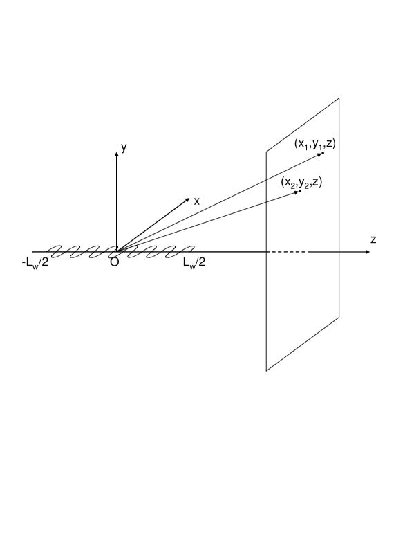
Figure 6: Illustration of the undulator geometry and of the observation plane.

The horizontally-polarized field produced by a single electron with offset $\vec{\hat{l}}$ and deflection $\vec{\hat{\eta}}$ in the far-zone (i.e. at $\hat{z}\gg 1$) can be represented by the scalar quantity:

$$\hat{E}_{f}\left(\hat{z},\vec{\hat{\eta}},\vec{\hat{l}},\vec{\hat{\theta}}\right) = \frac{1}{\hat{z}}\exp\left[i\left(\frac{\hat{z}\hat{\theta}^{2}}{2}-\vec{\hat{\theta}}\cdot\vec{\hat{l}}+\frac{\hat{l}^{2}}{2\hat{z}^{2}}~{}\right)\right]\Psi_{f}\left(\left|\vec{\hat{\theta}}-\frac{\hat{l}}{\hat{z}}-\vec{\hat{\eta}}\right|\right)~{},$$ (44)

where

$$\Psi_{f}(\alpha)\equiv\mathrm{sinc}\left[\frac{\alpha^{2}}{4}\right]~{},$$ (45)

subscript $f$ indicating the ”far-zone”. The field distribution of the virtual source positioned at $z=0$, corresponding to the waist of our laser-like beam was found to be:

$$\hat{{E}}_{0}\left(0,\vec{\hat{\eta}},\vec{\hat{l}},\vec{\hat{r}}\right) = -i\pi\exp\left[i\vec{\hat{\eta}}\cdot\left(\vec{\hat{r}}-\vec{\hat{l}}~{}\right)\right]\Psi_{0}\left({\left|~{}\vec{\hat{r}}-\vec{\hat{l}}~{}~{}\right|}\right)~{},$$ (46)

where

$$\Psi_{0}(\alpha)\equiv\frac{1}{\pi}\left[\pi-2\mathrm{Si}\left(\alpha^{2}\right)\right]~{}.$$ (47)

where $\mathrm{Si}(z)=\int_{0}^{z}dt\sin(t)/t$ indicates the sin integral function and subscript ”0” is indicative of the source position. Plots of $\Psi_{f}$ and $\Psi_{0}$ are given in Fig. 7 and Fig. 8. It should be noted here that the independent variable in both plots is the dummy variable $\alpha$. The characteristic transverse range of the field in the far zone is in units of the radiation diffraction angle $\sqrt{\lambdabar/L_{w}}$, while the characteristic transverse range of the field at the source is in units of the radiation diffraction size $\sqrt{\lambdabar L_{w}}$.

Figure 7: Universal function $\Psi_{f}(\alpha)$, used to calculate the far-zone radiation field of a single electron at the fundamental harmonic at perfect resonance.

Figure 8: Universal function $\Psi_{0}(\alpha)$, used to calculate the radiation field of a single electron at the fundamental harmonic at perfect resonance on the virtual source plane.

Finally, with the help of the Fresnel propagation formula Eq. (43), we found the following expression for the field distribution at any distance $\hat{z}>1/2$ from the virtual source:

$$\hat{E}\left(\hat{z},\vec{\hat{\eta}},\vec{\hat{l}},\vec{\hat{\theta}}\right) = \exp\left[\frac{i\hat{z}}{2}\left|\vec{\hat{\theta}}-\frac{\vec{\hat{l}}}{\hat{z}}~{}\right|^{2}\right]\Psi\left(\hat{z},\left|\vec{\hat{\theta}}-\frac{\vec{\hat{l}}}{\hat{z}}-\vec{\hat{\eta}}\right|\right)~{},$$ (48)

where we defined

$$\Psi(\hat{z},\alpha)\equiv\exp\left[-i\frac{\hat{z}\alpha^{2}}{2}\right]\left\{\mathrm{Ei}\left[\frac{i\hat{z}^{2}\alpha^{2}}{2{\hat{z}}-1}\right]-\mathrm{Ei}\left[\frac{i\hat{z}^{2}\alpha^{2}}{2{\hat{z}}+1}\right]\right\}~{},$$ (49)

and $\mathrm{Ei}(z)=-\int_{-z}^{\infty}dt\exp(-t)/t$ indicates the exponential integral function. Eq. (48) is a particular case of Eq. (41) at perfect resonance. Note that free space basically acts as a spatial Fourier transformation. This means that the field in the far zone is, aside for a phase factor, the Fourier transform of the field at any position $z$ down the beamline. It is also, aside for a phase factor, the spatial Fourier transform of the virtual source:

$${\hat{E}}_{0}\left(0,\vec{\hat{\eta}},\vec{\hat{l}},\vec{\hat{r}}\right) = -\frac{i\hat{z}}{2\pi}\int d\vec{\hat{\theta}}\exp{\left[-\frac{i|\vec{\hat{\theta}}|^{2}}{2}\hat{z}\right]}{\hat{E}}_{f}\left(\hat{z},\vec{\hat{\eta}},\vec{\hat{l}},\vec{\hat{\theta}}\right)\exp\left[{i}\vec{\hat{r}}\cdot\vec{\hat{\theta}}\right]~{}.$$ (50)

It follows that

$$\int d\vec{{\theta}}~{}\Psi_{f}(\theta)\exp{\left[{i}{\vec{\hat{r}}}\cdot\vec{{\theta}}\right]} = 2\pi\int_{0}^{\infty}d\theta~{}\theta J_{o}\left({|\vec{\hat{r}}}|\theta\right)\Psi_{f}(\theta)=2\pi^{2}\Psi_{0}\left(|\vec{\hat{r}}|\right)~{}.$$ (51)

We conclude verifying that Eq. (48) is in agreement with Eq. (44) and Eq. (46) $\hat{z}\gg 1$ and for $\hat{z}=0$, respectively. Consider first $\hat{z}=0$. For positive numbers $\alpha^{2}\equiv\left|\vec{\hat{r}}-\vec{\hat{l}}-\hat{z}\vec{\hat{\eta}}\right|^{2}>0$, we have

$$-i[\pi+2\mathrm{Si}(\alpha^{2})]=\mathrm{Ei}(-i\alpha^{2})-\mathrm{Ei}(i\alpha^{2})~{},$$ (52)

and Eq. (48) yields back Eq. (46).

Consider now the limit for $\hat{z}\gg 1$. For positive numbers $\xi^{2}\equiv\left|\vec{\hat{\theta}}-\vec{\hat{\eta}}\right|^{2}>0$ one has

$$\exp\left[-\frac{i\hat{z}\xi^{2}}{2}\right]\left[\mathrm{Ei}\left(\frac{i\xi^{2}\hat{z}^{2}}{2\hat{z}-1}\right)-\mathrm{Ei}\left(\frac{i\xi^{2}\hat{z}^{2}}{2\hat{z}+1}\right)\right]\longrightarrow\frac{1}{\hat{z}}\mathrm{sinc}\left(\frac{\xi^{2}}{4}\right)~{},$$ (53)

as it can be directly seen comparing Eq. (48) with Eq. (41)), where integration in Eq. (42) is performed directly at $\hat{C}=0$ and in the limit for $\hat{z}\gg 1$. Thus, Eq. (48) yields back Eq. (44), as it must be.

Finally, it should be noted that expressions in the present Section 2.4 have been derived for $\omega>0$. Expressions for the field at negative values of $\omega$ can be obtained based on the property $\vec{\bar{E}}(-\omega)=\vec{\bar{E}}^{*}(\omega)$ starting from explicit expressions at $\omega>0$.

2.5 Cross-spectral density of an undulator source and its free-space propagation.

From now on we consider a normalized expression of the cross-spectral density, $\hat{G}$, that is linked with $G$ in Eq. (17) by a proportionality factor

$$\hat{G}=\left(\frac{2c^{2}\gamma}{K\omega eA_{JJ}}\right)^{2}G~{}.$$ (54)

Moreover, we introduce variables

$$\Delta\vec{{r}}={\vec{\hat{r}}_{1}-\vec{\hat{r}}_{2}}~{},~{}~{}\vec{\bar{r}}=\frac{\vec{\hat{r}}_{1}+\vec{\hat{r}}_{2}}{2}~{}.$$ (55)

and

$$\Delta\vec{\theta}={\vec{\hat{\theta}}_{1}-\vec{\hat{\theta}}_{2}}~{},~{}~{}\vec{\bar{\theta}}=\frac{\vec{\hat{\theta}}_{1}+\vec{\hat{\theta}}_{2}}{2}~{},$$ (56)

where, as before, $\vec{\hat{\theta}}=\vec{\hat{r}}/z$. Thus, Eq. (17) can now be written as

$$\hat{G}(\hat{z},\vec{\bar{r}},\Delta\vec{r},\hat{C})\equiv\left\langle\hat{E}\left(\vec{\hat{\eta}},\vec{\hat{l}},\hat{z},\vec{\bar{r}}+\frac{\Delta\vec{r}}{2},\hat{C}\right)\hat{E}^{*}\left(\vec{\hat{\eta}},\vec{\hat{l}},\hat{z},\vec{\bar{r}}-\frac{\Delta\vec{r}}{2},\hat{C}\right)\right\rangle~{}.$$ (57)

On the one hand, the cross-spectral density as is defined in Eq. (57) includes the product of fields which obey the free space propagation relation Eq. (43). On the other hand, the averaging over random variables commutes with all operations involved in the calculation of the field propagation. More explicitly, introducing the notation $\hat{E}(z)=\mathcal{O}[\hat{E}(z_{s})]$ as a shortcut for Eq. (43) one can write

$$\hat{G}(z)=\left\langle\mathcal{O}\left[\hat{E}(\hat{z}_{s})\right]\mathcal{O}^{*}\left[\hat{E}^{*}(\hat{z}_{s})\right]\right\rangle=\mathcal{O}\cdot\mathcal{O}^{*}\left[\left\langle\hat{E}(\hat{z}_{s})\hat{E}^{*}(\hat{z}_{s})\right\rangle\right]=\mathcal{O}\cdot\mathcal{O}^{*}\left[G(\hat{z}_{s})\right]~{},$$ (58)

where $\mathcal{O}$ may also represent, more in general, any linear operator. Once the cross-spectral density at the source is known, Eq. (58) provides an algorithm to calculate the cross-spectral density at any position $\hat{z}$ down the beamline (in the free-space case). Similarly, propagation through a complex optical system can be performed starting from the knowledge of $\hat{G}(\hat{z}_{s})$. As a result, the main problem to solve in order to characterize the cross-spectral density at the specimen position is to calculate the cross-spectral density at the virtual source. For the undulator case, we fix the position of the source in the center of the undulator $\hat{z}_{s}=0$. This is the main issue this paper is devoted to. However, free-space propagation is also treated, and may be considered an illustration of how our main result can be used in a specific case.

Based on Eq. (57) and on results in Section 2.4 we are now ready to present an expression for the cross-spectral density at any position down the beamline, always keeping in mind that the main result we are looking for is the cross-spectral density at the virtual source position.

We begin giving a closed expression for $\hat{G}$ valid at any value of the detuning parameter $\hat{C}$ by substituting Eq. (41) in Eq. (57), and replacing the ensemble average with integration over the transverse beam distribution function. We thus obtain

$$\hat{G}\left(\hat{z},\hat{C},\vec{\bar{\theta}},\Delta\vec{\theta}\right)=\exp\left[{i\hat{z}\vec{\bar{\theta}}\cdot\Delta\vec{\theta}}\right]\int d\vec{\hat{l}}\exp\left[-{i}\vec{\hat{l}}\cdot\Delta\vec{\theta}\right]$$ (59)

$$\times\int d\vec{\hat{\eta}}f_{\bot}\left(\vec{\hat{l}},\vec{\hat{\eta}}\right){\Psi}_{C}\left(\hat{z},\hat{C},\left|\vec{\bar{\theta}}+\frac{\Delta\vec{\theta}}{2}-\frac{\vec{\hat{l}}}{\hat{z}}-\vec{\hat{\eta}}\right|\right){\Psi}^{*}_{C}\left(\hat{z},\hat{C},\left|\vec{\bar{\theta}}-\frac{\Delta\vec{\theta}}{2}-\frac{\vec{\hat{l}}}{\hat{z}}-\vec{\hat{\eta}}\right|\right)~{}.$$ (60)

(61)

It is often useful to substitute the integration variables $\vec{\hat{l}}$ with $\vec{\phi}\equiv-\vec{\bar{\theta}}+\vec{\hat{l}}/\hat{z}+\vec{\hat{\eta}}$ In fact, in this way, Eq. (61) becomes

$$\hat{G}\left(\hat{z},\hat{C},\vec{\bar{\theta}},\Delta\vec{\theta}\right)=\hat{z}^{2}\exp\left[{i\hat{z}\vec{\bar{\theta}}\cdot\Delta\vec{\theta}}\right]\int d\vec{\phi}\int d\vec{\hat{\eta}}\exp\left[-{i\hat{z}}\left(\vec{\phi}+\vec{\bar{\theta}}-\vec{\hat{\eta}}\right)\cdot\Delta\vec{\theta}\right]$$ (62)

$$\times f_{\bot}\left(\vec{\phi}+\vec{\bar{\theta}}-\vec{\hat{\eta}},\vec{\hat{\eta}}\right){\Psi}_{C}\left(\hat{z},\hat{C},\left|\vec{\phi}-\frac{\Delta\vec{\theta}}{2}\right|\right){\Psi}^{*}_{C}\left(\hat{z},\hat{C},\left|\vec{\phi}+\frac{\Delta\vec{\theta}}{2}\right|\right)~{},$$ (63)

For choices of $f$ of particular interest (e.g. product of Gaussian functions for both transverse and angle distributions), integrals in $d\vec{\eta}$ can be performed analytically, leaving an expression involving two integrations only, and still quite generic.

Eq. (63) is as far as we can get with this level of generality, and can be exploited with the help of numerical integration techniques. However, it still depends on six parameters at least: four parameters are needed to specify $f_{\bot}$, plus the detuning parameter $\hat{C}$ and the distance $\hat{z}$.

In the following we will assume $\hat{C}\ll 1$, that allows us to take advantage of analytical presentations for the single-particle field obtained in OURF and reported before. This means that monochromatization is good enough to neglect finite bandwidth of the radiation around the fundamental frequency. By this, we automatically assume that monochromatization is performed around the fundamental frequency. It should be noted, however, that our theory can be applied to the case monochromatization is performed at other frequencies too. Analytical presentation of the single-particle field cannot be used in full generality, but for any fixed value $\hat{C}$ of interest one may tabulate the special function $\Psi_{C}$ once and for all, and use it in place of $\Psi$ throughout the paper. From this viewpoint, although the case of prefect resonance studied here is of practical importance in many situations, it should be considered as a particular illustration of our theory only.

Also note that in Eq. (61) the electron beam energy spread is assumed to be negligible. Contrarily to the monochromator bandwidth, the energy spread is fixed for a given facility: its presence constitutes a fundamental effect. In order to quantitatively account for it, one should sum the dimensionless energy-spread parameter $\hat{\Delta}_{E}=4\pi N_{w}\delta\gamma/\gamma$ to $\hat{C}$ in Eq. (61) and, subsequently, integration should be extended over the energy-spread distribution. Typical energy spread $\delta\gamma/\gamma$ for third generation light sources is of order $0.1\%$. For ERL sources this figure is about an order of magnitude smaller, $\delta\gamma/\gamma\sim 0.01\%$.

Figure 9: Study of $\hat{I}$ given in Eq. (LABEL:enspread) for different valued of $\hat{C}$ and $\hat{\Delta}_{E}$. Here $N_{w}=70$. Plot (a) : comparison, at $\hat{C}=0$, of the case for negligible energy spread with the case $\hat{\Delta}_{E}=0.88$. Plot (b) : comparison, at negligible energy spread, of the case $\hat{C}=0$ with the case $\hat{C}=\pm 0.5$. Plot (c) : comparison of the case $\hat{C}=0$ at negligible energy spread with the case $\hat{C}=\pm 0.5$ at $\Delta\omega/\omega\simeq 0.1\%$.

In order to study the impact of a finite energy spread parameter $\hat{\Delta}_{E}$, of a finite radiation bandwidth and of a relatively small detuning from the fundamental we consider an expression for the intensity of a diffraction-limited beam $\hat{z}^{2}\hat{I}=\hat{z}^{2}\langle|\hat{E}|^{2}\rangle$ including both $\hat{\Delta}_{E}$ and $\hat{C}$:

$$\hat{z}^{2}\hat{I}(\hat{\theta},\hat{C},\hat{\Delta}_{E}) =\frac{1}{\sqrt{2\pi}\hat{\Delta}_{E}}\int_{-\infty}^{\infty}d\hat{\xi}_{E}\exp\left[-\frac{\hat{\xi}_{E}^{2}}{2\hat{\Delta}_{E}^{2}}\right]\mathrm{sinc}^{2}\left(\frac{\hat{C}+\hat{\xi}_{E}}{2}+\frac{\hat{\theta}^{2}}{4}\right)~{}.$$ (64)

We plotted $\hat{z}^{2}\hat{I}$ for different values of $\hat{C}$ and $\hat{\Delta}_{E}$ in Fig. 9. First, in Fig. 9 (a), we compared, at $\hat{C}=0$, the case for negligible energy spread with the case $\hat{\Delta}_{E}=0.88$, corresponding to $\delta\gamma/\gamma\simeq 0.1\%$ at $N_{w}=70$, typical of third generation sources. As one can see, maximal intensity differences are within $10\%$. Second, in Fig. 9 (b) we compared, at negligible energy spread, the case $\hat{C}=0$ with $\hat{C}=\pm 0.5$ at $N_{w}=70$, corresponding to a shift $\Delta\omega/\omega\simeq 0.1\%$. One can see that also in this case maximal intensities differ of about $10\%$. Analysis of Fig. 9 (c), where the case $\hat{C}=0$ at negligible energy spread is compared with cases $\hat{C}=\pm 0.5$ at $\Delta\omega/\omega\simeq 0.1\%$ and $N_{w}=70$ leads to a similar result. This reasoning allows to conclude that our simplest analytical illustrations can be applied to practical cases of interest involving third generation sources and undulators with up to $70$ periods with good accuracy. It should be remarked that such illustration holds for the first harmonic only. In fact, while the shape of $\hat{z}^{2}\hat{I}$ is still given by Eq. (LABEL:enspread) in the case of odd harmonic of order $h$, parameters $\hat{C}$ and $\hat{\Delta}_{E}$ are modified according to $\hat{C}_{h}=h\hat{C}$ and $\hat{\Delta}_{E~{}h}=h\hat{\Delta}_{E}$, decreasing the applicability of our analytical results.

With this in mind, we can present an expression for the cross-spectral density at $\hat{C}\ll 1$ based on Eq. (57) and Eq. (48). Substituting the latter in the former we obtain an equation for $\hat{G}(\hat{z},\vec{\bar{\theta}},\Delta\vec{\theta})$ that can be formally derived from Eq. (61) by substitution of $\Psi_{C}$ with $\Psi$. Similarly as before, one may give alternative presentation of $\hat{G}(\hat{z},\vec{\bar{\theta}},\Delta\vec{\theta})$ replacing the integration variables $\vec{\hat{l}}$ with $\vec{\phi}\equiv-\vec{\bar{\theta}}+\vec{\hat{l}}/\hat{z}+\vec{\hat{\eta}}$. This results in another expression for $\hat{G}(\hat{z},\vec{\bar{\theta}},\Delta\vec{\theta})$ that can be formally derived from Eq. (63) by substituting $\Psi_{C}$ with $\Psi$. This last expression presents the cross-spectral density in terms of a convolution of the transverse electron beam phase space distribution with an analytical function, followed by Fourier transformation.

One may obtain an expression for $\hat{G}$ at $\hat{z}=0$ as a limiting case of Eq. (61) or Eq. (63) at $\hat{C}=0$. It is however simpler to do so by substituting Eq. (46) in Eq. (57) that gives

$$\hat{G}\left(0,\vec{\bar{r}},\Delta\vec{r}\right) = \int d\vec{\eta}\exp\left[i\vec{{\eta}}\cdot\Delta\vec{r}\right]$$ (67)

$$\times\int d\vec{l}f_{\bot}\left(\vec{l},\vec{\eta}\right)\pi^{2}\Psi_{0}\left(\left|\vec{\bar{r}}-\frac{\Delta\vec{r}}{2}-\vec{l}\right|\right)\Psi_{0}\left(\left|\vec{\bar{r}}+\frac{\Delta\vec{r}}{2}-\vec{l}\right|\right)~{},$$

where the function $\Psi_{0}$ has already been defined in Eq. (47). The product $\Psi_{0}\left(\left|\vec{\bar{r}}-{\Delta\vec{r}}/{2}\right|\right)\Psi_{0}\left(\left|\vec{\bar{r}}+{\Delta\vec{r}}/{2}\right|\right)$ is a four-dimensional , analytical function in $\vec{\bar{r}}$ and $\Delta\vec{r}$. Eq. (67) tells that the cross-spectral density at the virtual source position can be obtained convolving $\Psi_{0}\left(\left|\vec{\bar{r}}-{\Delta\vec{r}}/{2}\right|\right)\Psi_{0}\left(\left|\vec{\bar{r}}+{\Delta\vec{r}}/{2}\right|\right)$ with the transverse beam distribution at $z=0$, $f_{\bot}\left(\vec{\hat{l}},\vec{\hat{\eta}}\right)$, considered as a function of $\vec{\hat{l}}$, and taking Fourier transform with respect to $\vec{\hat{\eta}}$. When the betatron functions have minima in the center of the undulator we have

$$f_{\bot}\left(\vec{\hat{l}},\vec{\hat{\eta}}\right)=f_{l}\left(\vec{\hat{l}}\right)f_{\eta}\left(\vec{\hat{\eta}}\right)~{}.$$ (68)

Then, Eq. (67) becomes

$$\hat{G}\left(0,\vec{\bar{r}},\Delta\vec{r}\right) = \int d\vec{\hat{\eta}}f_{\eta}\left(\vec{\hat{\eta}}\right)\exp\left[i\vec{\hat{\eta}}\cdot\Delta\vec{r}\right]$$ (70)

$$\times\int d\vec{\hat{l}}f_{l}\left(\vec{\hat{l}}\right)\pi^{2}\Psi_{0}\left(\left|\vec{\bar{r}}-\frac{\Delta\vec{r}}{2}-\vec{\hat{l}}\right|\right)\Psi_{0}\left(\left|\vec{\bar{r}}+\frac{\Delta\vec{r}}{2}-\vec{\hat{l}}\right|\right)~{},$$

that will be useful later on. In this case, the cross-spectral density is the product of two separate factors. First, the Fourier transform of the distribution of angular divergence of electrons. Second, the convolution of the transverse electron beam distribution with the four-dimensional function $\Psi_{0}\left(\left|\vec{\bar{r}}-{\Delta\vec{r}}/{2}\right|\right)\Psi_{0}\left(\left|\vec{\bar{r}}+{\Delta\vec{r}}/{2}\right|\right)$.

Eq. (61) (or Eq. (63)) constitutes the most general result in in the calculation of the cross-spectral density for undulator sources. Its applicability is not restricted to third generation light sources. In particular, it can be used for arbitrary undulator sources like ERLs EDGA or XFEL spontaneous undulators XFEL . Eq. (63) has been derived, in fact, under the only constraints $\gamma^{2}\gg 1$, $N_{w}\gg 1$ and $\sigma_{T}\omega_{r}\gg N_{w}$. Note that $\sigma_{T}\sim 30$ ps for a typical SR source, whereas $\sigma_{T}\sim 100$ fs for an XFEL spontaneous undulator source or an ERL. Yet, for all practical cases of interest, $\sigma_{T}\omega\gg N_{w}$. As we have seen before, Eq. (63) further simplifies in the particular but practical case of perfect resonance, i.e. in the limit for $\hat{C}\ll 1$. A particularly important asymptote of Eq. (61) at perfect resonance is at the virtual source position, described by Eq. (67), which express the cross-spectral density in the undulator center. While Eq. (61) (or Eq. (63)) solves all problems concerning characterization of transverse coherence properties of light in free-space, the knowledge of Eq. (67) constitutes, in the presence of optical elements, the first (and main) step towards the characterization of SR light properties at the specimen position. In fact, the tracking of the cross-spectral density can be performed with the help of standard statistical optics formalism developed for the solution of problems dealing with partially coherent sources. Finally, it should be noted that in the case of XFELs and ERLs, there is no further simplification that we may apply to previously found equations. In particular, the transverse electron beam phase space should be considered as the result of a start-to-end simulation or, better, of experimental diagnostics measurements in a operating machine. On the contrary, as we will see, extra-simplifications can be exploited in the case of third-generation light sources, allowing for the development of a more specialized theory.

Inspection of Eq. (61) or Eq. (67) results in the conclusion that a Gaussian-Schell model cannot be applied to describe partially coherent SR light. In fact, functions $\Psi_{C}$, $\Psi$, $\Psi_{0}$ and $\Psi_{f}$ are of non-Gaussian nature, as the laser-like beam they can be ascribed to is non-Gaussian. This explains our words in the Introduction, where we stated that COI1 , COI2 , COI3 are of general theoretical interest, but they do not provide a satisfactory approximation to third generation SR sources.

As a final remark to this Section, we should discuss the relation of our approach with that given, in terms of Wigner distribution, in KIM2 , KIM3 . As said in Section 1, treatment based on Wigner distribution is equivalent to treatment based on cross-spectral density. We chose to use cross-spectral density because such quantity is straightforwardly physically measurable, being related to the outcome of a Young’s experiment. Essentially, one can obtain a Wigner distribution $\hat{W}$ from $\hat{G}$ by means of an inverse Fourier transformation:

$$\hat{W}\left(\hat{z},\vec{\bar{r}},\vec{\bar{u}}\right)=\frac{1}{4\pi^{2}}\int d(\Delta\vec{r}~{})\exp\left[-i\Delta\vec{r}\cdot\vec{\bar{u}}\right]\hat{G}\left(\hat{z},\vec{\bar{r}},\Delta\vec{r}\right)~{}.$$ (71)

Thus, Eq. (70) gives

$$\hat{W}\left(0,\vec{\bar{r}},\vec{\bar{u}}\right) = \int d\vec{\hat{l}}\int d\vec{\hat{\eta}}f\left(\vec{\hat{l}},\vec{\hat{\eta}}\right)\hat{W}_{o}\left(0,\vec{\bar{r}}-\vec{\hat{l}},\vec{\bar{u}}-\vec{\hat{\eta}}\right)~{}.$$ (72)

where

$$\hat{W}_{o}\left(0,\vec{\alpha},\vec{\delta}\right)=\frac{1}{4}\int d(\Delta\vec{r}~{})\exp\left[-i\Delta\vec{r}\cdot\vec{\delta}\right]\Psi_{0}\left(\left|\vec{\alpha}-\frac{\Delta\vec{r}}{2}\right|\right)\Psi_{0}\left(\left|\vec{\alpha}+\frac{\Delta\vec{r}}{2}\right|\right)~{},$$ (73)

The Wigner distribution at $\hat{z}=0$ is presented as a convolution product between the electron phase-space and a universal function $\hat{W}_{o}$. This result may be directly compared (aside for different notation) with KIM2 , KIM3 , where the Wigner distribution is presented as a convolution between the electrons phase space and a universal function as well. The study in KIM2 , KIM3 ends at this point, presenting expressions for arbitrary detuning parameter. On the contrary, in the following Sections we will take advantage of expressions at perfect resonance, of small and large parameters related to third generation light sources and of specific characteristics of the electron beam distribution. This will allow us to develop a comprehensive theory of third generation SR sources.

3 Theory of transverse coherence for third-generation light sources

3.1 Cross-Spectral Density

We now specialize our discussion to third-generation light sources. We assume that the motion of particles in the horizontal and vertical directions are completely uncoupled. Additionally, we assume a Gaussian distribution of the electron beam in the phase space. These two assumptions are practically realized, with good accuracy, in storage rings. For simplicity, we also assume that the minimal values of the beta-functions in horizontal and vertical directions are located at the virtual source position $\hat{z}=0$, that is often (but not always) the case in practice. $f_{\bot}=f_{\eta_{x}}(\hat{\eta}_{x})f_{\eta_{x}}(\hat{\eta}_{y})f_{l_{x}}(\hat{l}_{x})f_{l_{x}}(\hat{l}_{y})$ with

$$f_{\eta_{x}}(\hat{\eta}_{x})=\frac{1}{\sqrt{2\pi D_{x}}}\exp{\left(-\frac{\hat{\eta}_{x}^{2}}{2D_{x}}\right)}~{},~{}~{}~{}~{}f_{\eta_{y}}(\hat{\eta}_{y})=\frac{1}{\sqrt{2\pi D_{y}}}\exp{\left(-\frac{\hat{\eta}_{y}^{2}}{2D_{y}}\right)}~{},$$ (74)

$$f_{l_{x}}(~{}\hat{l}_{x})=\frac{1}{\sqrt{2\pi N_{x}}}\exp{\left(-\frac{\hat{l}_{x}^{2}}{2N_{x}}\right)}~{},~{}~{}~{}~{}~{}f_{l_{y}}(~{}\hat{l}_{y})=\frac{1}{\sqrt{2\pi N_{y}}}\exp{\left(-\frac{\hat{l}_{y}^{2}}{2N_{y}}\right)}~{}.$$ (75)

Here

$$D_{x,y}=\frac{\sigma_{x^{\prime},y^{\prime}}^{2}}{{\lambdabar}/L_{w}}~{},~{}~{}~{}~{}~{}N_{x,y}=\frac{\sigma^{2}_{x,y}}{\lambdabar L_{w}}~{},$$ (76)

$\sigma_{x,y}$ and $\sigma_{x^{\prime},y^{\prime}}$ being rms transverse bunch dimensions and angular spreads. Parameters $N_{x,y}$ will be indicated as the beam diffraction parameters, are analogous to Fresnel numbers and correspond to the normalized square of the electron beam sizes, whereas $D_{x,y}$ represent the normalized square of the electron beam divergences. Consider the reduced emittances $\hat{\epsilon}_{x,y}=\epsilon_{x,y}/\lambdabar$, where $\epsilon_{x,y}$ indicate the geometrical emittance of the electron beam in the horizontal and vertical directions. Since we restricted our model to third generation light sources, we can consider $\hat{\epsilon}_{x}\gg 1$. Moreover, since betatron functions are of order of the undulator length, we can also separately accept

$$N_{x}\gg 1~{},~{}~{}~{}~{}~{}D_{x}\gg 1,$$ (77)

still retaining full generality concerning values of $N_{y}$ and $D_{y}$, due to the small coupling coefficient between horizontal and vertical emittance.

Exploitation of the extra-parameter $\hat{\epsilon}_{x}\gg 1$ (or equivalently $N_{x}\gg 1$ and $D_{x}\gg 1$) specializes our theory to the case of third-generation sources.

With this in mind we start to specialize our theory beginning with the expression for the cross-spectral density at the virtual source, i.e. Eq. (70). After the change of variables $\vec{\phi}\longrightarrow-\vec{\bar{r}}+\vec{\hat{l}}$, and making use of Eq. (75), Eq. (70) becomes

$$\hat{G}\left(0,\vec{\bar{r}},\Delta\vec{r}\right) = \frac{\pi}{2\sqrt{N_{x}N_{y}}}\exp\left[-\frac{(\Delta x)^{2}D_{x}}{2}\right]\exp\left[-\frac{(\Delta y)^{2}D_{y}}{2}\right]$$ (81)

$$\times\int_{-\infty}^{\infty}d\phi_{x}\int_{-\infty}^{\infty}d\phi_{y}\exp\left[-\frac{\left(\phi_{x}+\bar{x}\right)^{2}}{2N_{x}}\right]\exp\left[-\frac{\left(\phi_{y}+\bar{y}\right)^{2}}{2N_{y}}\right]$$

$$\times\Psi_{0}\left\{\left[\left({\phi_{x}}+\frac{\Delta x}{2}\right)^{2}+\left({\phi_{y}}+\frac{\Delta y}{2}\right)^{2}\right]^{1/2}\right\}$$

$$\times\Psi_{0}\left\{\left[\left({\phi_{x}}-\frac{\Delta x}{2}\right)^{2}+\left({\phi_{y}}-\frac{\Delta y}{2}\right)^{2}\right]^{1/2}\right\}~{},$$

where $\Delta x$ and $\Delta y$ indicate components of $\Delta\vec{r}$. In Eq. (81) the range of variable $\phi_{x}$ is effectively limited up to values $|\phi_{x}|\sim 1$. In fact, $\phi_{x}$ enters the expression for $\Psi_{0}$. It follows that at values larger than unity the integrand in Eq. (81) is suppressed. Then, since $N_{x}\gg 1$, we can neglect $\phi_{x}$ in the exponential function. Moreover $D_{x}\gg 1$ and from the exponential function in $D_{x}$ follows that $\Delta x\ll 1$ can be neglected in $\Psi_{0}$. As a result, Eq. (81) is factorized in the product of a horizontal cross-spectral density $G_{x}(0,\bar{x},\Delta x)$ and a vertical cross-spectral density $G_{y}(0,\bar{x},\Delta x)$:

$$\hat{G}\left(0,\vec{\bar{r}},\Delta\vec{r}\right)=\hat{G}_{x}\left(0,{\bar{x}},\Delta{x}\right)\hat{G}_{y}\left(0,{\bar{y}},\Delta{y}\right)~{},$$ (82)

where

$$\hat{G}_{x}\left(0,{\bar{x}},\Delta{x}\right) = \sqrt{\frac{\pi}{{N_{x}}}}\exp\left[-\frac{(\Delta x)^{2}D_{x}}{2}\right]\exp\left[-\frac{\bar{x}^{2}}{2N_{x}}\right]~{},$$ (83)

$$\hat{G}_{y}\left(0,{\bar{y}},\Delta{y}\right) = \frac{1}{2}\sqrt{\frac{\pi}{N_{y}}}\exp\left[-\frac{(\Delta y)^{2}D_{y}}{2}\right]\int_{-\infty}^{\infty}d\phi_{y}\int_{-\infty}^{\infty}d\phi_{x}\exp\left[-\frac{\left(\phi_{y}+\bar{y}\right)^{2}}{2N_{y}}\right]$$ (85)

$$\times\Psi_{0}\left\{\left[{\phi_{x}}^{2}+\left({\phi_{y}}+\frac{\Delta y}{2}\right)^{2}\right]^{1/2}\right\}\Psi_{0}\left\{\left[{\phi_{x}}^{2}+\left({\phi_{y}}-\frac{\Delta y}{2}\right)^{2}\right]^{1/2}\right\}~{}.$$

Note that, in virtue of Eq. (43), factorization holds in general, at any position $\hat{z}$. This allows us to separately study $\hat{G}_{x}$ and $\hat{G}_{y}$. $\hat{G}_{x}$ describes a quasi-homogeneous Gaussian source, which will be treated in Section 4.1. Here we will focus our attention on $\hat{G}_{y}$ only. It should be remarked that the quasi-homogenous Gaussian source asymptote is obtained from Eq. (LABEL:Gnor3y) in the limit $N_{y}\gg 1$ and $D_{y}\gg 1$. In other words, normalization constants in Eq. (83) and Eq. (LABEL:Gnor3y) are chosen in such a way that Eq. (LABEL:Gnor3y) reduces to Eq. (83) in the limit $N_{y}\gg 1$ and $D_{y}\gg 1$ (with the obvious substitution $x\longrightarrow y$). It should be clear that this normalization is most natural, but not unique. The only physical constraint that normalization of Eq. (83) and Eq. (LABEL:Gnor3y) should obey is that the product $\hat{G}_{x}\hat{G}_{y}$ should not change.

Let us define the two-dimensional universal function $\mathcal{S}(\alpha,\delta)$ as

$$\mathcal{S}(\alpha,\delta)=\mathcal{K}_{S}\int_{-\infty}^{\infty}d\phi_{x}\Psi_{0}\left\{\left[{\phi_{x}}^{2}+\left(\alpha+\frac{\delta}{2}\right)^{2}\right]^{1/2}\right\}\Psi_{0}\left\{\left[{\phi_{x}}^{2}+\left(\alpha-\frac{\delta}{2}\right)^{2}\right]^{1/2}\right\}~{}.$$ (87)

(88)

The normalization constant $\mathcal{K}_{S}\simeq 0.714$ is chosen in such a way that $\mathcal{S}(0,0)=1$. We can present $\hat{G}_{y}$ at the virtual source with the help of $\mathcal{S}$ as

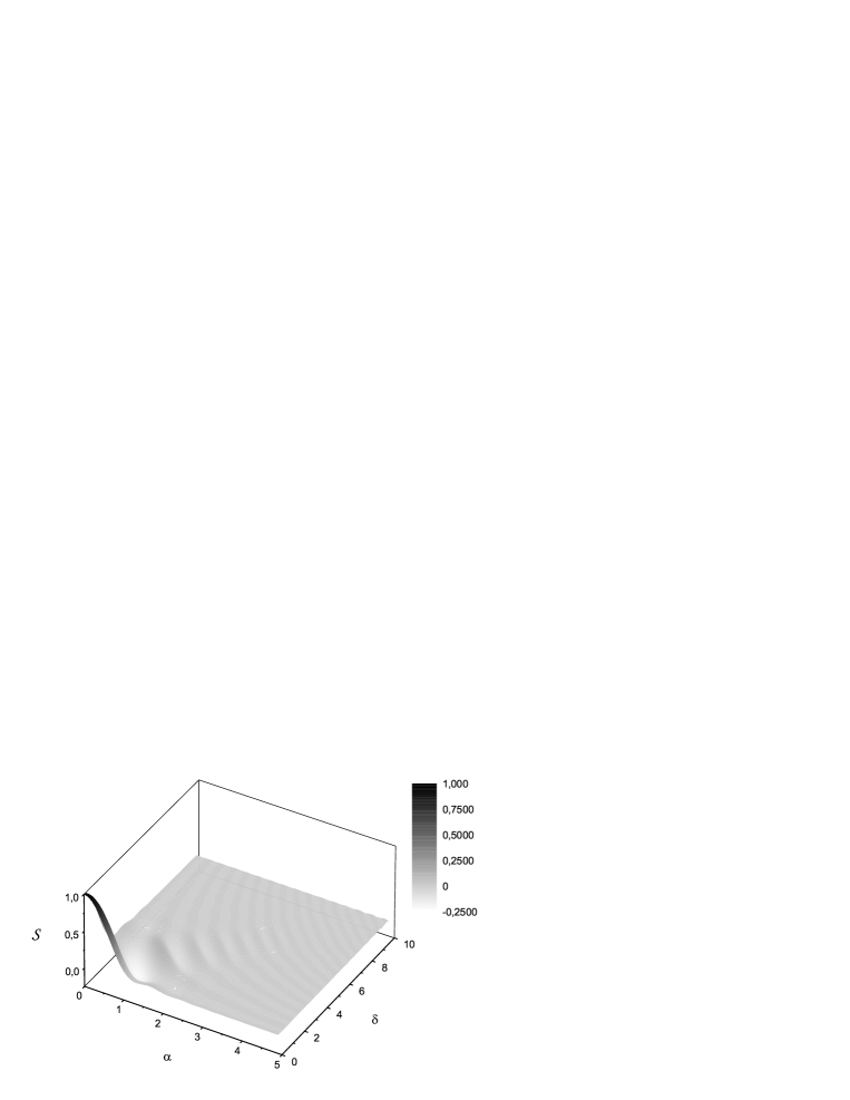
Figure 10: Plot of the universal function ${\mathcal{S}}$, used to calculate the cross-spectral density at the virtual source when $N_{x}\gg 1$, $D_{x}\gg 1$, $N_{y}$ and $D_{y}$ are arbitrary.

$$\hat{G}_{y}\left(0,{\bar{y}},\Delta{y}\right) = \frac{1}{2}\sqrt{\frac{\pi}{N_{y}}}\exp\left[-\frac{(\Delta y)^{2}D_{y}}{2}\right]\int_{-\infty}^{\infty}d\phi_{y}\exp\left[-\frac{\left(\phi_{y}+\bar{y}\right)^{2}}{2N_{y}}\right]$$ (90)

$$\times~{}\frac{1}{\mathcal{K}_{S}}\mathcal{S}(\phi_{y},\Delta y)~{}.$$

Therefore, $\hat{G}_{y}$ at the virtual source is found by convolving an universal function, $\mathcal{S}$, with a Gaussian function and multiplying the result by another Gaussian function.

Note that in the limit $N_{x}\gg 1$ and $D_{x}\gg 1$ there is no influence of the electron beam distribution along the vertical direction on $\hat{G}_{x}$. In spite of this, in the same limit, Eq. (90) shows that there is an influence of the horizontal electron beam distribution on $\hat{G}_{y}$, due to the non-separability of the function $\Psi_{0}$ in $\mathcal{S}$. In fact, contrarily to the case of a Gaussian laser beam, $\Psi_{0}[{\phi_{x}}^{2}+(\alpha-{\delta}/{2})^{2}]\neq\Psi_{0}[{\phi_{x}}^{2}]\Psi_{0}[(\alpha-{\delta}/{2})^{2}]$, and the integral in $d\phi_{x}$, that is a remainder of the integration along the x-direction, is still present in the definition of $\mathcal{S}$. However, such influence of the horizontal electron beam distribution is independent of $N_{x}$ and $D_{x}$. As a consequence, $\mathcal{S}$ is a universal function.

A plot of ${\mathcal{S}}$ is presented in Fig. 10. ${\mathcal{S}}$ is a real function. Then, $\hat{G}$ at the virtual plane is also real. Moreover, ${\mathcal{S}}$ is invariant for exchange of $\alpha$ with $\delta/2$.

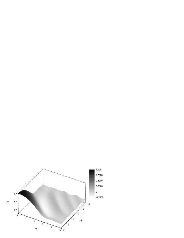
Figure 11: Plot of the universal function $\mathcal{F}$, used to calculate the cross-spectral density in the far zone when $N_{x}\gg 1$, $D_{x}\gg 1$, $N_{y}$ and $D_{y}$ are arbitrary.

Let us now deal with the evolution of the cross-spectral density $\hat{G}_{y}$ in free-space. In principle, one may use Eq. (90) and apply Eq. (58), remembering Eq. (43). It is however straightforward to use directly Eq. (63) at $\hat{C}\ll 1$. Under the assumption $N_{x}\gg 1$ and $D_{x}\gg 1$, as has been already remarked, factorization of $\hat{G}$ as a product of $\hat{G}_{x}$ and $\hat{G}_{y}$ holds for any value of $\hat{z}$. Isolating these factors in Eq. (63) at $\hat{C}\ll 1$ and using Eq. (75) one obtains

$$\hat{G}_{y}\left(\hat{z},{\bar{\theta}_{y}},\Delta{\theta}_{y}\right)=\frac{\hat{z}^{2}}{2\pi^{2}\sqrt{2N_{y}D_{y}}}\exp\left[{i\hat{z}\bar{\theta}_{y}\Delta{\theta}_{y}}\right]\int d{\phi}_{y}\exp\left[-{i\hat{z}}\left({\phi}_{y}+{\bar{\theta}_{y}}\right)\Delta{\theta}_{y}\right]$$ (91)

$$\times\int d\hat{\eta}_{y}\exp\left[i\hat{z}{\hat{\eta}_{y}}\Delta{\theta}_{y}\right]\exp\left[-\frac{\hat{\eta}_{y}^{2}}{2D_{y}}\right]\exp\left[-\frac{\left({\phi}_{y}+\bar{\theta}_{y}-\hat{\eta}_{y}\right)^{2}}{2N_{y}/\hat{z}^{2}}\right]$$ (92)

$$\times\int d\phi_{x}{\Psi}\left\{\hat{z},\left[{\phi}_{x}^{2}+\left(\phi_{y}-\frac{\Delta\theta_{y}}{2}\right)^{2}\right]^{1/2}\right\}{\Psi}^{*}\left\{\hat{z},\left[{\phi}_{x}^{2}+\left(\phi_{y}+\frac{\Delta\theta_{y}}{2}\right)^{2}\right]^{1/2}\right\}~{}.$$ (93)

The integral in $d\hat{\eta}_{y}$ (second line) can be calculated analytically yielding

$$\hat{G}_{y}\left(\hat{z},{\bar{\theta}}_{y},\Delta\theta_{y}\right)=\frac{\hat{z}}{2\pi\sqrt{\pi}\sqrt{N_{y}/\hat{z}^{2}+D_{y}}}\exp\left[{\hat{z}}{i\bar{\theta}_{y}\Delta\theta_{y}}\right]\exp\left[-\frac{D_{y}N_{y}\Delta\theta_{y}^{2}}{2\left(N_{y}/\hat{z}^{2}+D_{y}\right)}\right]$$ (94)

$$\times\int d{\phi}_{y}\exp\left[-\frac{i\left(\phi_{y}+\bar{\theta}_{y}\right)\Delta\theta_{y}N_{y}/\hat{z}}{N_{y}/\hat{z}^{2}+D_{y}}\right]\exp\left[-\frac{\left({\phi}_{y}+{\bar{\theta}_{y}}\right)^{2}}{2\left(N_{y}/\hat{z}^{2}+D_{y}\right)}\right]$$ (95)

$$\times\int d\phi_{x}{\Psi}\left\{\hat{z},\left[{\phi}_{x}^{2}+\left(\phi_{y}-\frac{\Delta\theta_{y}}{2}\right)^{2}\right]^{1/2}\right\}{\Psi}^{*}\left\{\hat{z},\left[{\phi}_{x}^{2}+\left(\phi_{y}+\frac{\Delta\theta_{y}}{2}\right)^{2}\right]^{1/2}\right\}~{}.$$ (96)

We are now interested in discussing the far-zone limit of Eq. (96). Up to now we dealt with the far-zone region of the field from a single particle, Eq. (44). In this case, the field exhibits a spherical wavefront. Such wavefront corresponds to the quadratic phase factor in Eq. (44). Note that when the electron is moving on-axis, Eq. (44) consists of the product of $\hat{z}^{-1}\exp[i\hat{z}\hat{\theta}^{2}/2]$ by a real function independent of $\hat{z}$. Such field structure can be taken as a definition of far-zone. A similar definition can be used for the far-zone pertaining the cross-spectral density. We regard the quadratic phase factor $\exp[{\hat{z}}{i\bar{\theta}_{y}\Delta\theta_{y}}]$ in Eq. (96) as the equivalent, in terms of cross-spectral density, of the quadratic phase factor for the single-particle field. We therefore take as definition of far-zone the region of parameters where $\hat{G}_{y}(\hat{z},\bar{\theta}_{y},\Delta\theta_{y})=\hat{z}^{-1}h(\bar{\theta}_{y},\Delta\theta_{y})\exp[{\hat{z}}{i\bar{\theta}_{y}\Delta\theta_{y}}]$, $h$ being a real function, and remains like that for larger values of $\hat{z}$.

Let us discuss the definition of the far-zone region in terms of problem parameters. In the single-particle situation, the only parameter of the problem was $\hat{z}$ and, as is intuitively sound, the far-zone region was shown to coincide with the limit $\hat{z}\gg 1$. In the case of Eq. (96), we deal with three parameters $\hat{z}$, ${N}_{y}$ and ${D}_{y}$. Therefore we should find that the far-zone is defined in terms of conditions involving all three parameters.

When $N_{y}\lesssim 1$ and $D_{y}\lesssim 1$, analysis of Eq. (96) shows that the far-zone region is for $\hat{z}\gg 1$. In this case the definition of far-zone for $\hat{G}_{y}$ coincides with that of far-zone for the field of a single particle.

However, when either or both $N_{y}\gg 1$ or $D_{y}\gg 1$ the situation is different, and one finds that the far-zone condition is a combination of $\hat{z}$, $N_{y}$, and $D_{y}$. In all these cases, detailed mathematical analysis of Eq. (96) shows that far-zone is reached when

$$\max[N_{y},1]\ll\hat{z}^{2}\max[D_{y},1]~{}.$$ (97)

As it will be clearer after reading Section 4.4, but can also be seen considering the definition of our dimensionless units, the physical meaning of comparisons of $N_{y}$ and $D_{y}$ with unity in condition (97) is that of a comparison between diffraction-related parameters (diffraction angle and diffraction size) and beam-related parameters (divergence and size of the electron beam).

When ${N}_{y}\gg 1$, but $D_{y}\lesssim 1$ condition (97) reads $\hat{z}^{2}\gg N_{y}\gg 1$. This result is in agreement with intuition. The far-zone condition for $\hat{G}_{y}$ does not coincide with that for the field of a single electron, but it is anyway reached far away from the source, at $\hat{z}\gg 1$. As we will see in Section 4.2, the case ${N}_{y}\gg 1$ with $D_{y}\lesssim 1$ corresponds to a quasi-homogeneous non-Gaussian source. In Section 4.2 we will see that in this case the VCZ theorem is applicable, and its region of applicability is in agreement with our definition of far-zone $\hat{z}^{2}\gg N_{y}\gg 1$.

When $D_{y}\gg 1$ (with arbitrary $N_{y}$) and condition (97) holds, analysis shows that the phase factor under the integral sign in Eq. (96) can be neglected. Moreover, in this case, the Gaussian function in $\phi_{y}+\bar{\theta}_{y}$ has a width in $\phi_{y}$ much larger than unity, while the integral in $d\phi_{x}$ in second line of Eq. (96) has a width in $\phi_{y}$ of order unity, because $\Psi$ does not depend on parameters. Therefore, the dependence in $\phi_{y}$ in the Gaussian function can always be omitted, and the Gaussian function factors out of the integral sign in $d\phi_{y}$. One is left with the product of exponential functions and the double integral

$$\tilde{f}(\Delta\theta_{y}) \equiv \int d{\phi}_{y}\int d\phi_{x}$$ (99)

$$\times{\Psi}\left\{\hat{z},\left[{\phi}_{x}^{2}+\left(\phi_{y}-\frac{\Delta\theta_{y}}{2}\right)^{2}\right]^{1/2}\right\}{\Psi}^{*}\left\{\hat{z},\left[{\phi}_{x}^{2}+\left(\phi_{y}+\frac{\Delta\theta_{y}}{2}\right)^{2}\right]^{1/2}\right\}~{},$$

which has a very peculiar property. In fact, it does not depend on $\hat{z}$. The proof is based on the autocorrelation theorem in two dimensions, and is given in detail in Appendix C of reference OURU . This quite remarkable property of $\tilde{f}$ carries the consequence that substitution of $\Psi$ with $\Psi_{f}$ can be performed in Eq. (LABEL:doubleint) without altering the final result.

When both $D_{y}\gg 1$ and $N_{y}\gg 1$, one may neglect the dependence in $\Delta\theta_{y}$ in functions $\Psi$ and $\Psi^{*}$ in Eq. (LABEL:doubleint), because the exponential function in $\Delta\theta_{y}$ before the integral sign limits the range of $\Delta\theta_{y}$ to values of order $1/\sqrt{N_{y}}\ll 1$. As a result, the double integration in $d\phi_{x}$ and $d\phi_{y}$ yields a constant, and the description of the photon beam is independent of $\Psi$, i.e. does not include diffraction effects. This result is intuitive: when the electron beam size and divergence is large compared to the diffraction size and divergence, the photon beam can be described in terms of the phase-space distribution of the electron beam. This approach will be treated in more detail in Section 4.4.

Finally, when $D_{y}\gg 1$ and $N_{y}\lesssim 1$, diffraction effects cannot be neglected, nor can be the dependence in $\Delta\theta_{y}$ in $\Psi$ and $\Psi^{*}$. In this case, from condition (97) we obtain that the far-zone coincides with $D_{y}\hat{z}^{2}\gg 1$. This result is completely counterintuitive. In fact, since $D_{y}\gg 1$, the far-zone is reached for values $\hat{z}\sim 1$, i.e. at the very end of the undulator. Yet, diffraction effects cannot be neglected, and the field from a single electron is far from exhibiting a spherical wavefront at $\hat{z}\sim 1$. This paradox is solved by the special property of the double integral in Eq. (LABEL:doubleint), that allows one to substitute $\Psi$ with $\Psi_{f}$ independently of the value of $\hat{z}$.

As it will be discussed in Section 4.1 and Section 4.2, the case $D_{y}\gg 1$ corresponds to a quasi-homogeneous Gaussian source when $N_{y}\gg 1$ and to a quasi-homogeneous non-Gaussian source when $N_{y}\lesssim 1$. It will be shown that the VCZ theorem is applicable to these situations. In particular, the applicability region of the VCZ theorem will be seen to be in agreement with our definition of far-zone.

Our discussion can be summarized in a single statement. The far zone is defined, in terms of problem parameters, by condition (97). Remembering this condition one can derive the far-zone expression for $\hat{G}_{y}$ simplifying Eq. (96):

$$\hat{G}_{y}(\hat{z},\bar{\theta}_{y},\Delta{\theta}_{y}) = \frac{1}{\hat{z}}\frac{1}{2\pi\sqrt{\pi D_{y}}}{\exp{\left[i\hat{z}\bar{\theta}_{y}\Delta{\theta}_{y}\right]}}\exp{\left[-\frac{N_{y}\Delta{\theta}_{y}^{2}}{2}\right]}$$ (102)

$$\times\int_{-\infty}^{\infty}d{\phi}_{y}\exp{\left[-\frac{(\bar{\theta}_{y}+{\phi}_{y})^{2}}{2D_{y}}\right]}\frac{1}{\mathcal{K}_{F}}\mathcal{F}\left({\phi}_{y},\Delta{\theta}_{y}\right)~{},$$

where the universal two-dimensional function $\mathcal{F}(\alpha,\delta)$ is normalized in such a way that $\mathcal{F}(0,0)=1$ and reads :

$$\mathcal{F}(\alpha,\delta) = \mathcal{K}_{F}{\int_{-\infty}^{\infty}d{\phi}_{x}\Psi_{f}\left\{\left[{{\phi}_{x}^{2}+\left(\alpha-\frac{\delta}{2}\right)^{2}}\right]^{1/2}\right\}}\Psi_{f}\left\{\left[{{\phi}_{x}^{2}+\left(\alpha+\frac{\delta}{2}\right)^{2}}\right]^{1/2}\right\}~{},$$ (103)

with $\mathcal{K}_{F}={3}/({8\sqrt{\pi}})$.

Note that, similarly to the source case, the right hand side of Eq. (102) is found by convolving an universal function, $\mathcal{F}$, with a Gaussian function and multiplying the result by another Gaussian function.

A plot of $\mathcal{F}$ function defined is given in Fig. 11. $\mathcal{F}$ is a real function. Thus, only the geometrical phase factor in Eq. (102) prevents $\hat{G}_{y}$ in the far-zone from being real. Another remarkable property of $\mathcal{F}$ is its invariance for exchange of $\alpha$ with $\delta/2$. Also, $\mathcal{F}$ is invariant for exchange of $\alpha$ with $-\alpha$ (or $\delta$ with $-\delta$).

Finally, from Eq. (51) and Eq. (88) we have

$${\mathcal{S}}(x,y)=\frac{\mathcal{K}_{S}}{4\pi^{3}\mathcal{K}_{F}}\int_{-\infty}^{\infty}d\alpha\int_{-\infty}^{\infty}d\delta\exp\left[2ix\alpha+\frac{iy\delta}{2}\right]\mathcal{F}(\alpha,\delta)~{}.$$ (105)

3.2 Intensity distribution

With expressions for the cross-spectral density at hand, it is now possible to investigate the intensity distribution along the beamline, letting $\Delta\vec{r}=0$ in the expression for $\hat{G}$. Since ${N}_{x}\gg 1$ and $D_{x}\gg 1$, factorization of the cross-spectral density still holds. Therefore we can investigate the intensity profile along the vertical direction without loss of generality.

Posing $\Delta y=0$ in Eq. (90) we obtain the intensity profile at the virtual source, $\hat{I}_{y}\left(0,{\bar{y}}\right)$, as a function of $\bar{y}$:

$$\hat{I}_{y}\left(0,{\bar{y}}\right) = \frac{1}{2\mathcal{K}_{S}}\sqrt{\frac{\pi}{N_{y}}}\int_{-\infty}^{\infty}d\phi_{y}\exp\left[-\frac{\left(\phi_{y}+\bar{y}\right)^{2}}{2N_{y}}\right]~{}\mathcal{I}_{S}(\phi_{y})~{},$$ (106)

where we introduced the universal function

$$\mathcal{I}_{S}(\alpha)\equiv\mathcal{S}(\alpha,0)=\mathcal{K}_{S}\int_{-\infty}^{\infty}d\phi_{x}\Psi_{0}^{2}\left(\sqrt{\phi_{x}^{2}+\alpha^{2}}\right)~{}.$$ (107)

A change of the integration variable: $\phi_{x}\longrightarrow x\equiv(\phi_{x}^{2}+\alpha^{2})^{1/2}$ allows the alternative representation:

$$\mathcal{I}_{S}(\alpha)=2\mathcal{K}_{S}\int_{0}^{\infty}dx\frac{\mathrm{rect}\left[\alpha/(2x)\right]}{\sqrt{1-\alpha^{2}/x^{2}}}\Psi_{0}^{2}\left(x\right)~{},$$ (108)

where the function $\mathrm{rect}(\xi)$ is defined following GOOD : it is equal to unity for $|\xi|\leqslant 1/2$ and zero otherwise.

Figure 12: The universal function ${\mathcal{I}_{S}}$, used to calculate intensity at the virtual-source position.

The intensity at the virtual-source position is given in terms of a convolution of a Gaussian function with the universal function $\mathcal{I}_{S}$. A plot of $\mathcal{I}_{S}$ is given in Fig. 12 .

Similar derivations can be performed in the far zone. Posing $\Delta\theta_{y}=0$ in Eq. (102) we obtain the directivity diagram of the radiation as a function of $\bar{\theta}_{y}$:

$$\hat{I}_{y}(\hat{z},\bar{\theta}_{y}) = \frac{1}{\hat{z}}\frac{1}{\sqrt{2\pi D_{y}}\mathcal{K}_{F}}\int_{-\infty}^{\infty}d{\phi}_{y}\exp{\left[-\frac{(\bar{\theta}_{y}+{\phi}_{y})^{2}}{2D_{y}}\right]}\mathcal{I}_{F}\left({\phi}_{y}\right)~{},$$ (109)

where we defined

$$\mathcal{I}_{F}(\alpha)\equiv\mathcal{F}\left(\alpha,0\right) = \mathcal{K}_{F}{\int_{-\infty}^{\infty}d{\phi}_{x}\Psi_{f}^{2}\left[\left({{\phi}_{x}^{2}+\alpha^{2}}\right)^{1/2}\right]}$$ (110)

$$= \mathcal{K}_{F}{\int_{-\infty}^{\infty}d{\phi}_{x}\mathrm{sinc}^{2}\left[\frac{{{\phi}_{x}^{2}+\alpha^{2}}}{4}\right]}~{}.$$ (111)

Figure 13: The universal function $\mathcal{I}_{F}$, used to calculate the intensity in the far zone.

The intensity in the far-zone is given in terms of a convolution of a Gaussian function with the universal function $\mathcal{I}_{F}$. A plot of $\mathcal{I}_{F}$ is given in Fig. 13.

3.3 Spectral degree of coherence

We can now present expressions for the spectral degree of coherence at the virtual source (that is a real quantity) and in the far-zone (that is not real). Eq. (19) can be written for the vertical direction and in normalized units as:

$$\hat{g}_{y}\left(\hat{z},{\bar{y}},\Delta y\right)=\frac{\hat{G}_{y}\left(\hat{z},{\bar{y}},\Delta{y}\right)}{\left[\hat{I}_{y}(\hat{z},\bar{y}+\Delta y/2)\right]^{1/2}\left[\hat{I}_{y}(\hat{z},\bar{y}-\Delta y/2)\right]^{1/2}}~{}.$$ (112)

Substitution of Eq. (90) and Eq. (106) in Eq. (112) gives the spectral degree of coherence at the virtual source:

$$\hat{g}_{y}\left(0,{\bar{y}},\Delta{y}\right) = \exp\left[-\frac{(\Delta y)^{2}D_{y}}{2}\right]\int_{-\infty}^{\infty}d\phi_{y}\exp\left[-\frac{\left(\phi_{y}+\bar{y}\right)^{2}}{2N_{y}}\right]~{}\mathcal{S}(\phi_{y},\Delta y)$$ (115)

$$\times\left\{\int_{-\infty}^{\infty}d\phi_{y}\exp\left[-\frac{\left(\phi_{y}+\bar{y}+\Delta y/2\right)^{2}}{2N_{y}}\right]~{}\mathcal{I}_{S}(\phi_{y})\right\}^{-1/2}$$

$$\times\left\{\int_{-\infty}^{\infty}d\phi_{y}\exp\left[-\frac{\left(\phi_{y}+\bar{y}-\Delta y/2\right)^{2}}{2N_{y}}\right]~{}\mathcal{I}_{S}(\phi_{y})\right\}^{-1/2}~{}.$$

Similarly, substitution of Eq. (102) and Eq. (109) in Eq. (112) gives the spectral degree of coherence in the far zone:

$$\hat{g}_{y}(\hat{z},\bar{\theta}_{y},\Delta{\theta}_{y}) = {\exp{\left[i\hat{z}\bar{\theta}_{y}\Delta{\theta}_{y}\right]}}\exp{\left[-\frac{(\Delta{\theta}_{y})^{2}N_{y}}{2}\right]}$$ (119)

$$\times\int_{-\infty}^{\infty}d{\phi}_{y}\exp{\left[-\frac{(\bar{\theta}_{y}+{\phi}_{y})^{2}}{2D_{y}}\right]}\mathcal{F}\left({\phi}_{y},\Delta{\theta}_{y}\right)$$

$$\times\left\{\int_{-\infty}^{\infty}d{\phi}_{y}\exp{\left[-\frac{(\bar{\theta}_{y}+\Delta\theta_{y}/2+{\phi}_{y})^{2}}{2D_{y}}\right]}\mathcal{I}_{F}\left({\phi}_{y}\right)\right\}^{-1/2}$$

$$\times\left\{\int_{-\infty}^{\infty}d{\phi}_{y}\exp{\left[-\frac{(\bar{\theta}_{y}-\Delta\theta_{y}/2+{\phi}_{y})^{2}}{2D_{y}}\right]}\mathcal{I}_{F}\left({\phi}_{y}\right)\right\}^{-1/2}~{}.$$

3.4 Influence of horizontal emittance on vertical coherence for $D_{y}\ll 1$ and $N_{y}\ll 1$

The theory developed up to now is valid for arbitrary values of $N_{y}$ and $D_{y}$. In the present Section 3.4 we discuss an application in the limiting case for ${D}_{y}\ll 1$ and ${N}_{y}\ll 1$ corresponding to third generation light sources operating in the soft X-ray range.

At the virtual source position, the following simplified expression for the spectral degree of coherence in the vertical direction is derived from Eq. (115):

$$\hat{g}_{y}\left(0,{\bar{y}},\Delta{y}\right)=\mathcal{X}_{S}({\bar{y}},\Delta{y})~{},$$ (120)

where

$$\mathcal{X}_{S}(\alpha,\delta)=\frac{{\mathcal{S}}(\alpha,\delta)}{\left[{\mathcal{I}_{S}}(\alpha-\delta/2)\right]^{1/2}\left[{\mathcal{I}_{S}}(\alpha+\delta/2)\right]^{1/2}}~{}.$$ (121)

Thus, $\hat{g}_{y}$ is given by the universal function $\mathcal{X}_{S}$. A plot of $\mathcal{X}_{S}$ is given in Fig. 14.

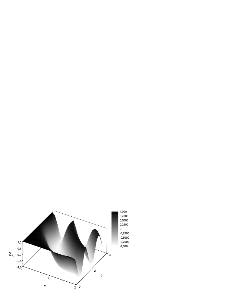
Figure 14: Plot of the universal function $\mathcal{X}_{S}$, used to calculate the modulus of the spectral degree of coherence of the source when $\hat{N}_{x}\gg 1$, $\hat{D}_{x}\gg 1$, $\hat{N}_{y}\ll 1$ and $\hat{D}_{y}\ll 1$.

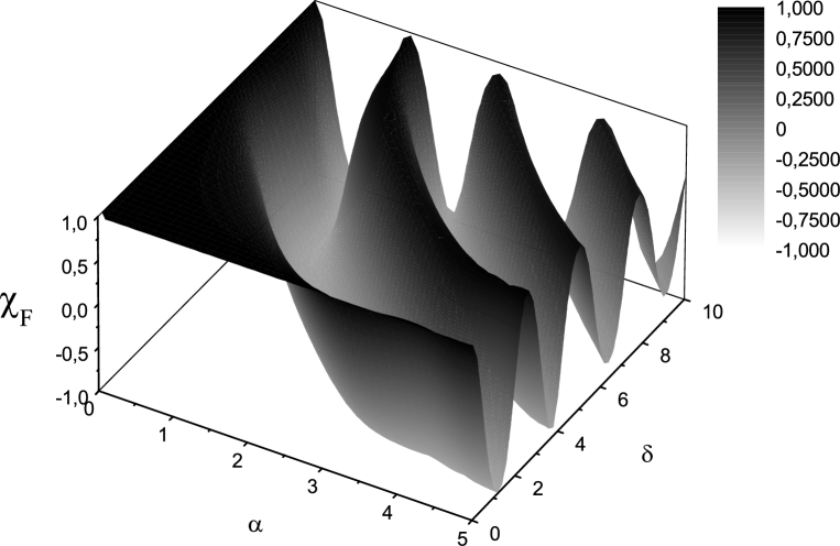
Figure 15: Plot of the universal function $\mathcal{X}_{F}$, used to calculate the modulus of the spectral degree of coherence in the far zone when $\hat{N}_{x}\gg 1$, $\hat{D}_{x}\gg 1$, $\hat{N}_{y}\ll 1$ and $\hat{D}_{y}\ll 1$.

Similarly, in the far zone, one obtains from Eq. (119):

$$\hat{g}_{y}(\hat{z},\bar{\theta}_{y},\Delta{\theta}_{y}) = {\exp{\left[i\hat{z}\bar{\theta}_{y}\Delta{\theta}_{y}\right]}}\mathcal{X}_{F}({\bar{\theta}_{y}},\Delta\theta_{y})~{}.$$ (122)

Here the universal function $\mathcal{X}_{F}$ is given by

$$\mathcal{X}_{F}{\left(\alpha,\delta\right)}=\frac{\mathcal{F}(\alpha,\delta)}{\left[\mathcal{I}_{F}(\alpha-\delta/2)\right]^{1/2}\left[\mathcal{I}_{F}(\alpha+\delta/2)\right]^{1/2}}~{}.$$ (123)

Thus, $|\hat{g}_{y}|$ is given by the universal function $\mathcal{X}_{F}$. A plot of $\mathcal{X}_{F}$ is presented in Fig. 15 as a function of dummy variable $\alpha$ and $\delta$. It is straightforward to see that $\mathcal{X}_{F}({\bar{\theta}_{y}},\Delta\theta_{y})$ is symmetric with respect to $\Delta{\theta}_{y}$ and with respect to the exchange of $\Delta{\theta}_{y}/2$ with $\bar{\theta}_{y}$. When $\bar{\theta}_{y}=0$, i.e. $\hat{\theta}_{y1}=-\hat{\theta}_{y2}$, we obviously obtain $\mathcal{X}_{F}(0,\Delta{\theta}_{y})=1$ that corresponds to complete coherence at this particular value of $\bar{\theta}_{y}$. However, since $|\hat{g}_{y}|=\mathcal{X}_{F}$ oscillates from positive to negative values, in general one never has full coherence in the vertical direction, even in the case of zero vertical emittance. Note that this effect does not depend, in the limit for ${N}_{x}\gg 1$ and ${D}_{x}\gg 1$, on the actual values of ${N}_{x}$ and ${D}_{x}$.

Figure 16: Comparison between some zeros of $\mathcal{X}_{F}$, at coordinates $(\bar{\theta}_{y},\Delta{\theta}_{y}$ (black circles), and the directivity diagram of undulator radiation in the vertical direction at very large horizontal electron beam divergence $\hat{D}_{x}\gg 1$ and negligible vertical divergence $\hat{D}_{y}\ll 1$ (solid line).

In other words, as it is evident from Fig. 15, $\mathcal{X}_{F}({\bar{\theta}_{y}},\Delta\theta_{y})$ exhibits many different zeros in $\bar{\theta}_{y}$ for any fixed value of $\Delta{\theta}_{y}$. In Fig. 16 some of these zeros are illustrated with black circles on the plane $(\bar{\theta}_{y},\Delta{\theta}_{y})$. Consider a two-pinhole experiment as in Fig. 4. Once a certain distance $\hat{z}\Delta{\theta}_{y}$ between the two pinholes is fixed, Fig. 16 illustrates at what position of the pinhole system, $\bar{\theta}_{y}$, the spectral degree of coherence in the vertical direction drops from unity to zero for the first time.

To estimate the importance of this effect, it is crucial to consider the position of $\bar{\theta}_{y}$ in the directivity diagram of the radiant intensity, that coincides in this case with $\mathcal{I}_{F}(\bar{\theta}_{y})$ (solid line in Fig. 16). From Fig. 16 one can see that $\mathcal{X}_{F}({\bar{\theta}_{y}},\Delta\theta_{y})$ drops to zero for the first time at $\Delta{\theta}_{y}\sim 2$ $\bar{\theta}_{y}\sim 2$, where the X-ray flux is still intense. This behavior of the degree of coherence may influence particular kind of experiments. To give an example we go back to the two-pinhole setup in Fig. 4. After spatial filtering in the horizontal direction, one will find that for some vertical position $\bar{\theta}_{y}$ of the pinholes (at fixed $\Delta{\theta}_{y}$), well within the radiation pattern diagram, there will be no fringes, while for some other vertical position there will be perfect visibility. Without the knowledge of the function $\mathcal{X}_{F}$ it would not be possible to fully predict the outcomes of a two-pinhole experiment. Results described here should be considered as an illustration of our general theory that may or may not, depending on the case under study, have practical influence. It may, however, be the subject of experimental verification.

3.4.1 Discussion

Although the $\mathcal{X}_{F}$ is independent of $N_{x}$ and $D_{x}$, its actual shape is determined by the presence of a large horizontal emittance. Let us show this fact. If both $N_{x,y}\ll 1$ and $D_{x,y}\ll 1$ (filament beam limit), one would have had $|\hat{G}|=\Psi_{f}\left(\left|\vec{\theta}_{1}\right|\right)\Psi_{f}\left(\left|\vec{\theta_{2}}\right|\right)$, so that $|\hat{g}|=1$, strictly. Note that in this case $\hat{G}$ could not be factorized. When instead $N_{x}\gg 1$ and $D_{x}\gg 1$ the cross-spectral density can be factorized according to Eq. (82), but the integration in $d\phi_{x}$, that follows from an integration over the horizontal electron beam distribution, is still included in the vertical cross-spectral density $\hat{G}_{x}$ (and, therefore, in $\mathcal{X}_{F}$). This results in the outcome described above and can be traced back to the non-Gaussian nature of $\Psi_{f}$. Note that if one adopted a Gaussian-Schell model, the cross-spectral density could have been split in the product of Gaussian intensity and Gaussian spectral degree of coherence and $\Psi_{f}$, being a product of Gaussians, would have been separable. Then, $|\hat{g}_{y}|$ would have been constant for $N_{x}\gg 1$ and $D_{x}\gg 1$. As a result, the effect described here would not have been recognized. This fact constitutes a particular realization of our general remarks about Gaussian-Schell models at the end of Section 2.5.

As a final note to the entire Section, we stress the fact that our theory of partial coherence in third generation light sources is valid under several non-restrictive assumptions. Alongside with previously discussed conditions $\gamma^{2}\gg 1$, $N_{w}\gg 1$, $\sigma_{T}\omega\gg N_{w}$ and the assumption of perfect resonance (i.e. the limit $\hat{C}\ll 1$), we assumed separability and particular shape of the electron beam phase space (see Eq. (75)). Moreover, for third generation light sources we assumed $\epsilon_{x}\gg\lambdabar$ (up to the VUV range). Together with $\beta_{x,y}\simeq L_{w}$ this implies $N_{x}\gg 1$ and $D_{x}\gg 1$, allowing for separability of the cross-spectral density in horizontal and vertical factors. Moreover, due to $N_{x}\gg 1$ and $D_{x}\gg 1$, we are dealing with quasi-homogenous Gaussian sources in the horizontal direction. This particular kind of sources will be treated in detail as an asymptote of our general theory in the next Section. In the vertical direction instead, we still have fully generic sources. We showed how the vertical cross-spectral density can be expressed in terms of convolutions between two-dimensional universal functions and Gaussian functions. A particularly interesting case is that of quasi-homogeneous non-Gaussian sources that will also be treated as an asymptotic case in the following Section dedicated to quasi-homogeneous sources.

4 Quasi-homogeneous asymptotes for undulator sources

In Section 3 we developed a general theory of transverse coherence properties of third generation light sources. In this Section we consider the class of quasi-homogeneous sources for undulator devices as an asymptotic limit for that theory.

Quasi-homogeneous sources are defined by the fact that the cross-spectral density of the virtual source (positioned at $z=0$) can be written as:

$$\hat{G}\left(0,\vec{\bar{r}},\Delta\vec{r}\right)=\hat{I}\left(0,\vec{\bar{r}}\right)\hat{g}\left(\Delta\vec{r}\right)~{}.$$ (124)

The definition of quasi-homogeneity amounts to a factorization of the cross-spectral density as the product of the field intensity distribution and the spectral degree of coherence. A set of necessary and sufficient conditions for such factorization to be possible follows: (i) the radiation intensity at the virtual source varies very slowly with the position across the source on the scale of the field correlation length and (ii) the spectral degree of coherence depends on the positions across the source only through the difference $\Delta\vec{r}$.

Factorization of Eq. (81) as in Eq. (124), for third generation light sources, is equivalent to a particular choice of the region of parameters for the electron beam: ${N}_{x}\gg 1$, ${D}_{x}\gg 1$ and either (or both) ${N}_{y}\gg 1$ and ${D}_{y}\gg 1$. In this case, the reader may verify that conditions (i) and (ii) are satisfied.

In the horizontal direction, we have both $N_{x}\gg 1$ and $D_{x}\gg 1$ for wavelengths up to the VUV range, so that factorization of the cross-spectral density in horizontal and vertical contributions $\hat{G}_{x}$ and $\hat{G}_{y}$ always holds.

Let us first consider $\hat{G}_{y}$. Depending on the values of $N_{y}$ and $D_{y}$ we may have Gaussian quasi-homogeneous sources characterized by a Gaussian transverse distribution of intensity ($N_{y}\gg 1$ and $D_{y}\gg 1$), as well as non-Gaussian quasi-homogeneous sources ($N_{y}\gg 1$ and $D_{y}\lesssim 1$ or $N_{y}\lesssim 1$ and $D_{y}\gg 1$). Gaussian quasi-homogenous sources are to be expected in the vertical direction in the hard X-ray limit, where diffraction effects play no role. On the contrary, diffraction effects must be accounted for when dealing with non-Gaussian quasi-homogeneous sources.

Let us now consider $\hat{G}_{x}$. In the horizontal direction both $N_{x}\gg 1$ and $D_{x}\gg 1$. It follows that Gaussian quasi-homogeneous sources find a very natural application in the description of the cross-spectral density in the horizontal direction, from the hard X-ray to the VUV range.

We will see that the VCZ theorem applies to all quasi-homogeneous cases. Actually, the concept of far-zone for quasi-homogeneous sources can be introduced as the region in the parameter space $\hat{z},N_{x,y},D_{x,y}$ such that the VCZ theorem holds. We will see that these condition coincides with condition (97) given before.

4.1 Gaussian undulator sources

When $N_{x}\gg 1$ and $D_{x}\gg 1$ Eq. (83) applies. When $N_{y}\gg 1$ and $D_{y}\gg 1$, Eq. (LABEL:Gnor3y) reduces to

$$\hat{G}_{y}\left(0,{\bar{y}},\Delta{y}\right) = \sqrt{\frac{\pi}{{N_{y}}}}\exp\left[-\frac{(\Delta y)^{2}D_{y}}{2}\right]\exp\left[-\frac{\bar{y}^{2}}{2N_{y}}\right]~{},$$ (125)

that is equivalent to Eq. (83): thus, identical treatments hold separately in the horizontal and vertical directions. For this reasons, and for simplicity of notation, we drop all subscripts ”x” or ”y” in the present Section 4.1, and we substitute letters ”x” and ”y” in variables with the more generic ”r”. However, as stated before, the Gaussian quasi-homogeneous model primarily describes third generation light sources in the horizontal direction.

Eq. (124) is satisfied. Moreover,

$$\hat{I}\left(0,{\bar{r}}\right)=\sqrt{\frac{\pi}{{N}}}\exp\left[-\frac{\bar{r}^{2}}{2N}\right]$$ (126)

and

$$\hat{g}(\Delta r)=\exp\left[-\frac{(\Delta r)^{2}D}{2}\right]~{}.$$ (127)

Propagation of Eq. (125) can be found taking the limit of Eq. (96) for $N\gg 1$ and $D\gg 1$, which yields an analytical expression for the evolution of the cross-spectral density based on Eq. (63) at $\hat{C}\ll 1$ :

$$\hat{G}(\hat{z},\bar{r},\Delta r) = \frac{\sqrt{\pi}}{{\hat{z}\sqrt{A+D}}}\exp\left[-\frac{\bar{r}^{2}}{2({A}+{D})\hat{z}^{2}}\right]\exp\left[i\frac{\bar{r}\Delta{r}}{\hat{z}}\right]$$ (129)

$$\times\exp\left[-i\frac{{A}\bar{r}\Delta{r}}{\hat{z}({A}+{D})}\right]\exp\left[-\frac{{A}{D}(\Delta r)^{2}}{2({A}+{D})}\right]~{},$$

where

$${A}=\frac{{N}}{\hat{z}^{2}}~{}.$$ (130)

We have

$$\hat{I}(\hat{z},\bar{r}) = \frac{\sqrt{\pi}}{{\hat{z}\sqrt{A+D}}}\exp\left[-\frac{\bar{r}^{2}}{2({A}+{D})\hat{z}^{2}}\right]~{},$$ (131)

and

$$\hat{g}(\hat{z},\Delta r) = \exp\left[i\frac{\bar{r}\Delta{r}}{\hat{z}}\right]\exp\left[-i\frac{{A}\bar{r}\Delta{r}}{\hat{z}({A}+{D})}\right]\exp\left[-\frac{{A}{D}(\Delta r)^{2}}{2({A}+{D})}\right]~{}.$$ (132)

Note that, due to the phase factors in Eq. (129), only the virtual source at $\hat{z}=0$ constitutes a quasi-homogeneous source.

Geometrical interpretation of ${A}$ is the dimensionless square of the apparent angular size of the electron bunch at the observer point position, calculated as if the beam was positioned at $\hat{z}=0$.

The far-zone for quasi-homogeneous Gaussian sources is given by condition $A\ll D$, which can be retrieved by condition (97) or directly by Eq. (129). In this case, simplification of Eq. (129) or use of Eq. (102) in the limit for $N\gg 1$ and $D\gg 1$ yields the far-zone cross-spectral density:

$$\hat{G}\left(\hat{z},{\bar{\theta}},\Delta{\theta}\right) = \frac{1}{\hat{z}}\sqrt{\frac{\pi}{D}}\exp\left[i\hat{z}{\bar{\theta}}\Delta{\theta}\right]\exp\left[-\frac{N(\Delta\theta)^{2}}{2}\right]\exp\left[-\frac{\bar{\theta}^{2}}{2D}\right]~{},$$ (133)

so that

$$\hat{I}\left(\hat{z},{\bar{\theta}}\right) = \frac{1}{\hat{z}}\sqrt{\frac{\pi}{D}}\exp\left[-\frac{\bar{\theta}^{2}}{2D}\right]~{},$$ (135)

and

$$\hat{g}\left(\hat{z},\Delta{\theta}\right) = \exp\left[i\hat{z}{\bar{\theta}}\Delta{\theta}\right]\exp\left[-\frac{N(\Delta\theta)^{2}}{2}\right]~{}.$$ (136)

Similarly as before we suppressed subscripts ”x” or ”y” in the symbol $\theta$.

Analysis of Eq. (125) and Eq. (LABEL:Gnorgaussf) allows to conclude that

$(a_{2})$ the spectral degree of coherence of the field at the source plane $g({\Delta{r}})$ and the angular distribution of the radiant intensity $I({\bar{\theta}})$ are a Fourier pair.

$(b_{2})$ the spectral degree of coherence of the far field $g(\Delta{\theta})$ and the source-intensity distribution $I({\bar{r}})$ are, apart for a simple geometrical phase factor, a Fourier pair.

The statement $(b_{2})$ is a version of the VCZ theorem valid for quasi-homogeneous sources. Statement $(a_{2})$ instead, regards the symmetry between space and angle domains, and can be seen as an inverse VCZ theorem.

This discussion underlines the link between the VCZ theorem and the Wiener-Khinchin theorem. Exactly as the space domain has a reciprocal description in terms of transverse (two-dimensional) wave vectors, the time domain has a reciprocal description in terms of frequency. The reader will recognize the analogy between statements $(a_{2})$ and $(b_{2})$, with statements $(a_{1})$ and $(b_{1})$ discussed in Section 2.3. In particular, the VCZ is analogous to the inverse Wiener-Khincin theorem. Similarly, separability of $G$ in Eq. (124) in the product of spectral degree of coherence and intensity is analogous to separability of $\Gamma_{\omega}$, in Eq. (16) in the product of spectral correlation function and spectral density distribution of the source.

Let us calculate the transverse coherence length $\hat{\xi}_{c}$ as a function of the observation distance $\hat{z}$. We introduce the coherence length following the definition by Mandel WOLF . The coherence length, naturally normalized to the diffraction length $\sqrt{L_{w}c/\omega}$ is defined as

$$\hat{\xi}_{c}(\hat{z})=\int_{-\infty}^{\infty}|g(\hat{z},\Delta r)|^{2}d(\Delta r)~{},$$ (137)

Performing the integration in Eq. (137) with the help of Eq. (132) yields:

$$\hat{\xi}_{c}(\hat{z})={\sqrt{\pi}}\left(\frac{1}{{A}}+\frac{1}{{D}}\right)^{1/2}~{}.$$ (138)

Figure 17: Coherence length $\hat{\xi}_{c}$ as a function of $\hat{z}$ and asymptotic behaviors for $\hat{z}\longrightarrow 1/2$ and $\hat{z}\gg 1$. Here ${N}=10^{3}$ and ${D}=10$.

The coherence length in Eq. (138) exhibits linear dependence on $\hat{z}$, that is $\hat{\xi}_{c}\longrightarrow\sqrt{\pi/{N}}~{}{\hat{z}}$ while for $\hat{z}\longrightarrow 1/2$ that is at the end of the undulator, it converges to a constant $\hat{\xi}_{c}\longrightarrow[\pi/(4{N})+\pi/{D}]^{1/2}$. Eq. (138) and its asymptotes are presented in Fig. 17 for the case ${N}=10^{3}$, ${D}=10$. At the exit of the undulator, $\hat{\xi}_{c}\sim 1/\sqrt{{D}}$, because ${N}\gg{D}$. On the other hand, horizontal dimension of the light spot is simply proportional to $\sqrt{{N}}$. This means that the horizontal dimension of the light spot is determined by the electron beam size, as is intuitive, while the beam angular distribution is printed in the fine structures of the intensity function that are of the dimension of the coherence length. In the limit for $A\ll D$ the situation is reversed. The radiation field at the source can be presented as a superposition of plane waves, all at the same frequency $\omega$, but with different propagation angles with respect to the $z$-direction. Since the radiation at the exit of the undulator is partially coherent, a spiky angular distribution of intensity is to be expected. The nature of the spikes is easily described in terms of Fourier transform theory. From Fourier transform theorem we can expect an angular spectrum with Gaussian envelope and rms width $\sqrt{{D}}$. Also, the angular distribution of intensity should contain spikes with characteristic width $1/\sqrt{N}$, as a consequence of the reciprocal width relations of Fourier transform pairs (see Fig. 18). This is realized in mathematics by the expression for the cross-spectral density, Eq. (129) and by the equation for the coherence length, Eq. (138).

It is also important to remark that the asymptotic behavior for ${A}\ll 1$ of $\hat{g}$, that is Eq. (136) and $\hat{\xi}_{c}$, that is

$$\hat{\xi}_{c}\longrightarrow\sqrt{\frac{\pi}{N}}{\hat{z}}$$ (139)

Figure 18: Physical interpretation of the generalized VCZ theorem. If the radiation beyond the source plane is partially coherent, a spiky angular distribution of intensity is expected. The nature of these spikes is easily described in Fourier transform notations. We can expect that typical width of the angular distribution of intensity should be of order $(\omega\Delta/c)^{-1}$, where $\Delta$ is the typical linear dimension of spatially random intensity fluctuations. If the source has transverse size $d$, the angular distribution of intensity should contain spikes with typical width of about $(\omega d/c)^{-1}$, a consequence of the reciprocal width relations of Fourier transform pairs.

are direct application of VCZ theorem. In fact, the last exponential factor on the right hand side of Eq. (129) is simply linked with the Fourier transform of $f_{{l}}\left(\hat{l}\right)$. We derived Eq. (129) for ${N}\gg 1$ and ${D}\gg 1$, with $A\ll D$: in non-normalized units these conditions mean that the VCZ theorem is applicable when the electron beam divergence is much larger than the diffraction angle, i.e. $\sigma^{\prime 2}\gg\lambda/(2\pi L_{w})$, the electron beam dimensions are much larger than the diffraction size, i.e. $\sigma^{2}\gg\lambda L_{w}/2\pi$, and $({\sigma^{\prime}}{z})^{2}\gg{\sigma}^{2}$.

In GOOD (paragraph 5.6.4) a rule of thumb is given for the applicability region of the generalization of the VCZ theorem to quasi-homogeneous sources. The rule of thumb requires $z>2d\Delta/\lambda$ where $d$ is ”the maximum linear dimension of the source”, that is the diameter of a source with uniform intensity and $\Delta$ ”represents the maximum linear dimension of a coherence area of the source”. In our case, since $\sigma$ is the rms source dimension, $d\simeq 2\sigma$. Moreover, from Eq. (138) we have $\Delta=\xi_{c}\simeq\lambda/(2\sqrt{\pi}\sigma^{\prime})$. The rule of thumb then requires $z>2\sigma/(\sqrt{\pi}\sigma^{\prime})$: in dimensionless form this reads $\hat{z}\gtrsim\sqrt{{N}/{D}}$. This is parametrically in agreement with our limiting condition $A\ll D$, even though these two conditions are different when it come to actual estimations: our condition $A\ll D$ is, in fact, only an asymptotic one. To see how well it works in reality we might consider the plot in Fig. 17. There ${N}=10^{3}$ and ${D}=10$. Following GOOD we may conclude that a good condition for the applicability of the VCZ theorem should be $\hat{z}\gtrsim 10$. However as it is seen from the figure, the linear asymptotic behavior is not yet a good approximation at $\hat{z}\simeq 10$. This may be ascribed to the fact that the derivation in GOOD is not generally valid, but has been carried out for sources which drop to zero very rapidly outside the maximum linear dimension $d$ and whose correlation function also drops rapidly to zero very rapidly outside maximum linear dimension $\Delta$. However, at least parametrically, the applicability of the VCZ theorem in the asymptotic limit $A\ll D$ can be also expected from the condition $z>2d\Delta/\lambda$ in GOOD .

We conclude that the far field limit ${A}\ll{D}$ corresponds with the applicability region of the VCZ theorem. When this is the case, the VCZ theorem applies and the modulus of the spectral degree of coherence in the far field, forms a Fourier pair with the intensity distribution of the virtual source. In particular one concludes that the rms width of the virtual source is $\sqrt{N}$. In our study case for $N\gg 1$ and $D\gg 1$, such a relation between the rms width of the spectral degree of coherence in the far field and the rms dimension of the virtual source is also a relation between the rms width of the cross-spectral density function in the far field and the rms dimension of the electron beam at the plane of minimal beta function in the center of the undulator. In dimensional units one can write the value $\sigma_{c}$ of the rms width of the spectral degree of coherence $\hat{g}(\Delta\vec{r})$ in the far field as

$$\sigma_{c}=\frac{\lambda z}{2\pi\sigma}~{}.$$ (140)

Here $\sigma$ is, as usual, the rms dimension of the electron beam. These few last remarks help to clarify what is the size of the source in the VCZ theorem, that is far from being a trivial question. In several papers YAB1 , PFEI the rms electron beam size is recovered from the measurement of the transverse coherence length and subsequent application of the VCZ theorem, under the assumptions that the VCZ theorem can indeed be applied. In this regard, in YAB1 Section V, one may find a statement according to which the rms electron beam size ”is only the average value along the undulator” because ”the beta function has a large variation along the undulator”. Another example dealing with the same issue is given in reference PFEI . This paper (as well as reference YAB1 ) reports experimental results. However, authors of PFEI observe a disagreement between the electron beam rms size reconstructed from the VCZ theorem and beam diagnostics result of about a factor $2$. They ascribe this variation to the variation of the electron beam size along the undulator. In footnote 25 of reference PFEI , one may read: ”The precise shape and width of the x-ray intensity distribution in the source plane are directly connected to the properties of the electron beam. It would not be surprising if the limited depth of focus of the parabolically shaped electron beta function in the undulator translates into a virtually enlarged x-ray source size.”. At first glance it looks like if the SR source had a finite longitudinal dimension, and the virtual source size depended on variations of the beta function along the undulator. However, as we have seen before, the concept of virtual source involves a single transverse plane, and in the most general case any variation of the beta function does not affect the virtual source size. In our case of quasi-homogeneous Gaussian source, the virtual source is located where the beta function is minimal, and its size coincides with the transverse size of the electron beam at that location.

Finally, it should be remarked that the VCZ theorem can only be applied to quasi-homogeneous sources. Consider for example YAB1 , YAB2 , where a characterization of the vertical emittance in Spring-8 is reported, based on the measurement of the X-Ray beam coherence length in the far zone. The experiment was performed at the beamline BL29XU. Based on the assumption of validity of the VCZ theorem, it was found that the rms electron beam size at the undulator center (corresponding to the minimal value of the beta function) was $s_{y}\simeq 4.5~{}\mu$m, and that the coupling factor between horizontal and vertical emittance was down to the value $\zeta\simeq 0.12\%$, which corresponds to an extremely small vertical emittance $\epsilon_{y}=3.6$ pm$\cdot$rad. A resolution limit of this method was also discussed, based on numerical calculations of the radiation size from a single electron performed at the exit of the undulator, $s_{p}\simeq 1.6~{}\mu$m at $E_{p}=14.41$ keV for the $4.5$ m long undulator used in the experiment. The resolution limit of the measurement of $s_{y}$ was estimated to be about $1~{}\mu$m. Considering propagation laws for Gaussian beams it seems reasonable that the radiation spot size at the virtual source, located in the center of the undulator, be smaller than $s_{p}$. However, undulator radiation from a single electron cannot be considered a Gaussian beam. In particular, under the resonance approximation the field at the exit of the undulator exhibits a singularity and is not suitable for evaluation of the radiation spot size.

Use of $s_{p}$ led to an underestimation of the virtual source size and, thus, an overestimation of the resolution. Let us show this fact. Based on Eq. (46), we can determine the correct virtual source size of undulator radiation from a single electron. Let us consider the case when the single electron is emitting photons at the fundamental harmonic with energy $E=14.41$ keV. The angular frequency of light oscillations is given, in this case, by $\omega=2.2\cdot 10^{19}$ Hz. For an undulator length $L_{w}=4.5$ m, the normalization factor for the transverse size, $(L_{w}c/\omega)^{1/2}$, is about $8~{}\mu$m. From Fig. 8 obtain the dimensionless Half Width Half Maximum (HWHM) radiation size from a single electron (i.e. the HWHM width of the intensity distribution at the virtual source, located at the center of the undulator). This HWHM dimensionless value is about $0.7$. It follows that the HWHM value of the radiation spot size from a single electron is about $0.7\cdot(cL_{w}/\omega)^{1/2}\simeq 6~{}\mu$m. Therefore, the resolution in YAB1 , YAB2 , is estimated to be better than the correct value.

Note that the HWHM radiation spot size from a single electron is larger than the rms electron beam size $s_{y}\simeq 4.5~{}\mu$m found by means of coherence measurements. One concludes that the uncertainty due to finite resolution is larger than the measured electron beam size. This suggests that the analysis of experimental results YAB1 , YAB2 might include a logical flaw. Authors of that reference assume the validity of the VCZ theorem in the vertical direction. If one assumes their result of a vertical emittance ${\epsilon}_{y}\simeq 0.3\lambda/(2\pi)$, it follows a posteriori that the VCZ theorem could not have been applied in first instance (in this experiment the value of the beta function was ${\beta}\simeq L_{w}$). We suggest that analysis of experimental results in YAB1 , YAB2 should be based, instead, on the study of transverse coherence for non-homogeneous undulator sources in free space made in the previous Section 3.

4.2 Non-Gaussian undulator sources

Let us now turn to the analysis of non-Gaussian quasi-homogeneous sources on the basis of Eq. (LABEL:Gnor3y) and Eq. (102). We still assume that $N_{x}\gg 1$ and $D_{x}\gg 1$. Moreover, as before, we assume that the minimal beta function is located at the undulator center.

4.2.1 Case of a large electron-beam size $N_{y}\gg 1$ and $D_{y}\lesssim 1$.

Eq. (LABEL:Gnor3y) simplifies to

$$\hat{G}_{y}\left(0,{\bar{y}},\Delta{y}\right) = \sqrt{\frac{\pi}{N_{y}}}\exp\left[-\frac{(\Delta y)^{2}D_{y}}{2}\right]\exp\left[-\frac{\bar{y}^{2}}{2N_{y}}\right]\gamma_{S}(\Delta y)~{},$$ (141)

where we defined the universal function $\gamma_{S}(\alpha)$ as

$$\gamma_{S}(\alpha) = \frac{1}{2}\int_{-\infty}^{\infty}d\phi_{y}\int_{-\infty}^{\infty}d\phi_{x}\Psi_{0}\left\{\left[{\phi_{x}}^{2}+\left({\phi_{y}}+\frac{\alpha}{2}\right)^{2}\right]^{1/2}\right\}\Psi_{0}\left\{\left[{\phi_{x}}^{2}+\left({\phi_{y}}-\frac{\alpha}{2}\right)^{2}\right]^{1/2}\right\}$$ (144)

$$=\frac{1}{2\mathcal{K}_{S}}\int_{-\infty}^{\infty}d\phi_{y}\mathcal{S}(\phi_{y},\alpha)~{}.$$

Figure 19: Plot of the universal function $\gamma_{S}(\alpha)$, used to calculate the cross-spectral density of a quasi-homogeneous source when ${N}_{x}\gg 1$, ${D}_{x}\gg 1$, ${N}_{y}\gg 1$ and ${D}_{y}\lesssim 1$.

A plot of $\gamma_{S}(\alpha)$ is given in Fig. 19. Main features of $\gamma_{S}$ are a strong non-Gaussian shape, and the fact that also negative values are assumed. Eq. (124) is satisfied. Moreover,

$$\hat{I}_{y}\left(0,{\bar{y}}\right) = \sqrt{\frac{\pi}{N_{y}}}\exp\left[-\frac{\bar{y}^{2}}{2N_{y}}\right]~{},$$ (145)

and

$$\hat{g}_{y}\left(0,\Delta{y}\right) = \exp\left[-\frac{(\Delta y)^{2}D_{y}}{2}\right]\gamma_{S}(\Delta y)~{},$$ (147)

In the far-zone, Eq. (102) simplifies to

$$\hat{G}_{y}(\hat{z},\bar{\theta}_{y},\Delta{\theta}_{y}) = \frac{1}{2\pi\hat{z}\sqrt{\pi D_{y}}\mathcal{K}_{F}}{\exp{\left[i\hat{z}\bar{\theta}_{y}\Delta{\theta}_{y}\right]}}\exp{\left[-\frac{N_{y}\Delta{\theta}_{y}^{2}}{2}\right]}$$ (150)

$$\times\int_{-\infty}^{\infty}d\hat{\phi}_{y}\exp{\left[-\frac{(\bar{\theta}_{y}+\hat{\phi}_{y})^{2}}{2D_{y}}\right]}\mathcal{I}_{F}(\phi_{y})~{},$$

where $\mathcal{I}_{F}$ has already been defined in Eq. (13). Moreover,

$$\hat{I}_{y}(\hat{z},\bar{\theta}_{y}) = \frac{1}{2\pi\hat{z}\sqrt{\pi D_{y}}\mathcal{K}_{F}}\int_{-\infty}^{\infty}d\hat{\phi}_{y}\exp{\left[-\frac{(\bar{\theta}_{y}+\hat{\phi}_{y})^{2}}{2D_{y}}\right]}\mathcal{I}_{F}(\phi_{y})~{},$$ (151)

and

$$\hat{g}_{y}(\hat{z},\Delta{\theta}_{y}) = {\exp{\left[i\hat{z}\bar{\theta}_{y}\Delta{\theta}_{y}\right]}}\exp{\left[-\frac{N_{y}\Delta{\theta}_{y}^{2}}{2}\right]}~{}$$ (152)

Note that, due to geometrical phase factor in Eq. (150), only the virtual source at $\hat{z}=0$ constitutes a quasi-homogeneous source.

Also, $\gamma_{S}$ and $\mathcal{I}_{F}$ basically form a Fourier pair:

$$\gamma_{S}(\Delta{y})=\frac{1}{{2}\pi^{2}\mathcal{K}_{F}}\int_{-\infty}^{\infty}d{\phi}_{y}\exp{\left[i\Delta{y}{\phi}_{y}\right]}\mathcal{I}_{F}({\phi}_{y})~{},$$ (153)

meaning that the inverse VCZ theorem is satisfied for $N_{x,y}\ll\hat{z}^{2}$.

Finally, it is possible to calculate $\gamma_{S}$ analytically. To this purpose, it is sufficient to note that the Fourier transform

$${\widetilde{\gamma}}_{S}(\xi,\eta)=\int_{-\infty}^{\infty}d\hat{\phi}_{x}\int_{-\infty}^{\infty}d\hat{\phi}_{y}\exp{\left[i(\xi\hat{\phi}_{x}+\eta\hat{\phi}_{y})\right]}\mathrm{sinc}^{2}\left(\frac{\hat{\phi}_{x}^{2}+\hat{\phi}_{y}^{2}}{4}\right)~{}$$ (154)

can be evaluated with the help of the Bessel-Fourier formula as

$${\widetilde{\gamma}}_{S}(\lambda) = 2\pi\int_{0}^{\infty}d{\phi}~{}{\phi}J_{0}\left({\phi}\lambda\right)\mathrm{sinc}^{2}\left(\frac{{\phi}^{2}}{4}\right)$$ (155)

$$= 2\pi\left[\pi+\lambda^{2}\mathrm{Ci}\left(\frac{\lambda^{2}}{2}\right)-2\sin\left(\frac{\lambda^{2}}{2}\right)-2\mathrm{Si}\left(\frac{\lambda^{2}}{2}\right)\right]~{},$$ (156)

where $\lambda^{2}=\xi^{2}+\eta^{2}$, $\phi^{2}=\phi_{x}^{2}+\phi_{y}^{2}$, $\mathrm{Si}(\cdot)$ is the sine integral function and $\mathrm{Ci}(\cdot)$ is the cosine integral function. Thus, letting $\xi=0$ and $\eta=\Delta y$ one has

$$\gamma_{S}(\Delta{y})=\frac{1}{\pi}\left[\pi+(\Delta y)^{2}\mathrm{Ci}\left(\frac{(\Delta y)^{2}}{2}\right)-2\sin\left(\frac{(\Delta y)^{2}}{2}\right)-2\mathrm{Si}\left(\frac{(\Delta y)^{2}}{2}\right)\right]~{}.$$ (157)

4.2.2 Case of a large electron-beam divergence $D_{y}\gg 1$ and $N_{y}\lesssim 1$.

A similar analysis can be given in the case of a large electron-beam divergence. In this case Eq. (LABEL:Gnor3y) simplifies to give

$$\hat{G}_{y}\left(0,{\bar{y}},\Delta{y}\right) = \frac{1}{2\mathcal{K}_{S}}\sqrt{\frac{\pi}{N_{y}}}\exp\left[-\frac{(\Delta y)^{2}D_{y}}{2}\right]\int_{-\infty}^{\infty}d\phi_{y}\exp\left[-\frac{\left(\phi_{y}+\bar{y}\right)^{2}}{2N_{y}}\right]\mathcal{I}_{S}(\phi_{y})~{},$$ (158)

where $\mathcal{I}_{S}$ has already been defined in Eq. (108). Eq. (124) is satisfied. Moreover,

$$\hat{I}_{y}\left(0,{\bar{y}}\right) = \frac{1}{2\mathcal{K}_{S}}\sqrt{\frac{\pi}{N_{y}}}\int_{-\infty}^{\infty}d\phi_{y}\exp\left[-\frac{\left(\phi_{y}+\bar{y}\right)^{2}}{2N_{y}}\right]\mathcal{I}_{S}(\phi_{y})~{},$$ (160)

$$\hat{g}_{y}\left(0,\Delta{y}\right) = \exp\left[-\frac{(\Delta y)^{2}D_{y}}{2}\right]~{}.$$ (162)

In the far zone, Eq. (102) simplifies to

$$\hat{G}(\hat{z},\bar{\theta}_{y},\Delta{\theta}_{y}) = \frac{1}{\hat{z}}\sqrt{\frac{\pi}{D_{y}}}{\exp{\left[i\hat{z}\bar{\theta}_{y}\Delta{\theta}_{y}\right]}}\exp{\left[-\frac{N_{y}\Delta{\theta}_{y}^{2}}{2}\right]}\exp{\left[-\frac{\bar{\theta}_{y}^{2}}{2D_{y}}\right]}\gamma_{F}(\Delta\theta_{y})~{},$$ (164)

where

$$\gamma_{F}(\alpha) = \frac{1}{2\pi^{2}}\int_{-\infty}^{\infty}d{\phi}_{y}\int_{-\infty}^{\infty}d{\phi}_{x}$$ (168)

$$\times\Psi_{f}\left\{\left[{{\phi}_{x}^{2}+\left(\phi_{y}-\frac{\alpha}{2}\right)^{2}}\right]^{1/2}\right\}\Psi_{f}\left\{\left[{{\phi}_{x}^{2}+\left(\phi_{y}+\frac{\alpha}{2}\right)^{2}}\right]^{1/2}\right\}$$

$$=\frac{1}{2\pi^{2}\mathcal{K}_{F}}\int_{-\infty}^{\infty}d\phi_{y}\mathcal{F}(\phi_{y},\alpha)~{}.$$

Moreover

$$\hat{I}_{y}(\hat{z},\bar{\theta}_{y}) = \frac{1}{\hat{z}}\sqrt{\frac{\pi}{D_{y}}}\exp{\left[-\frac{\bar{\theta}_{y}^{2}}{2D_{y}}\right]}~{},$$ (169)

and

$$\hat{g}(\hat{z},\Delta{\theta}_{y}) = {\exp{\left[i\hat{z}\bar{\theta}_{y}\Delta{\theta}_{y}\right]}}\exp{\left[-\frac{N_{y}\Delta{\theta}_{y}^{2}}{2}\right]}\gamma_{F}(\Delta\theta_{y}),$$ (171)

Figure 20: Plot of the universal function $\gamma_{F}$, used to calculate the cross-spectral density in the far zone when $\hat{N}_{x}\gg 1$, $\hat{D}_{x}\gg 1$, $\hat{N}_{y}\lesssim 1$ and $\hat{D}_{y}\gg 1$.

A plot of $\gamma_{F}(\alpha)$ is given in Fig. 20. As for $\gamma_{S}$, main features of $\gamma_{F}$ are a strong non-Gaussian shape, and the fact that also negative values are assumed. Due to the phase factors in Eq. (LABEL:nong2f), only the virtual source at $\hat{z}=0$ constitutes a quasi-homogeneous source.

Also, $\mathcal{I}_{S}$ and $\gamma_{F}$ form a Fourier pair:

$${\mathcal{I}_{S}}(\bar{y})=\frac{\mathcal{K}_{S}}{\pi}\int_{-\infty}^{\infty}d{\phi}_{y}\exp\left[-i\bar{y}{\phi}_{y}\right]\gamma_{F}({\phi}_{y})~{},$$ (173)

meaning that the VCZ theorem is satisfied for $\hat{z}^{2}D_{x,y}\gg 1$. Since $D_{x,y}\gg 1$ this means that, in this case, the far zone begins at the very exit of the undulator, at $\hat{z}\sim 1$.

Finally, starting with the representation of $\mathcal{I}_{S}$ in Eq. (108), we can write (see GOOD Appendix A.3.)

$${\mathcal{I}_{S}}(\bar{y})=\mathcal{K}_{S}\int_{-\infty}^{\infty}d{\phi}_{y}\exp\left[-i\bar{y}{\phi}_{y}\right]\int_{0}^{\infty}d\alpha~{}\alpha J_{0}(\alpha\phi_{y})\Psi_{0}^{2}(\alpha)~{}.$$ (174)

Comparison with Eq. (173) yields the following alternative representation of $\gamma_{F}$ in terms of a one-dimensional integral involving special functions:

$$\gamma_{F}(\phi_{y})=\pi\int_{0}^{\infty}d\alpha~{}\alpha J_{0}(\alpha\phi_{y})\Psi_{0}^{2}(\alpha)~{}.$$ (175)

4.3 Accuracy of the quasi-homogeneous approximation

As we have discussed before, the quasi-homogeneous approximation can be applied when either or both $N_{y}\gg 1$ or $D_{y}\gg 1$. In this Section we will see that the accuracy of the quasi-homogeneous approximation scales as $(\sqrt{\max[N_{y},1]\max[D_{y},1]}~{})^{-1}$. As we have previously seen, in the particular case when both $N_{y}\gg 1$ and $D_{y}\gg 1$, a Gaussian model may be used. We will see that the accuracy of such model is worse than that of the quasi-homogeneous model, and scales as $\max(1/\sqrt{D_{y}},1/\sqrt{N_{y}})$.

We begin demonstrating that, when the source is quasi-homogeneous, we may take the approximation $\hat{\mathcal{S}}(\Delta{y},\hat{\phi})\simeq\gamma_{S}(\Delta{y})\mathcal{I}_{S}(\hat{\phi})$ in Eq. (90) with an accuracy scaling as $(\sqrt{\max[N_{y},1]\max[D_{y},1]}~{})^{-1}$. First, let us introduce a normalized version of the one-dimensional inverse Fourier transform of the function $\mathcal{F}$, that is

$$\bar{\mathcal{F}}(u,v) = \frac{1}{2\pi^{2}\mathcal{K}_{F}}\int_{-\infty}^{\infty}\mathcal{F}\left(\alpha,v\right)\exp\left[2iu\alpha\right]d\alpha=\frac{1}{2\mathcal{K}_{S}}\int_{-\infty}^{\infty}{\mathcal{S}}\left(u,\delta\right)\exp\left[-iv\frac{\delta}{2}\right]d\delta,$$ (176)

where the normalization factor is chosen in such as way that $\bar{\mathcal{F}}(0,0)=1$. The cross-spectral density in Eq. (90) can therefore be written as

$$\hat{G}_{y}(0,\bar{y},\Delta{y}) = \frac{1}{4\sqrt{2}\pi^{2}}\exp\left[-\frac{{D}_{y}(\Delta{y}^{2})}{2}\right]$$ (179)

$$\times\int_{-\infty}^{\infty}d{u}\exp\left[-i\frac{{u}\bar{y}}{2}\right]\exp\left[-\frac{{N}_{y}{u}^{2}}{2}\right]\bar{\mathcal{F}}(\Delta{y},{u})~{},$$

having used the convolution theorem. Under the quasi-homogeneous assumption, we can approximate $\bar{\mathcal{F}}(\Delta{y},{u})\simeq\bar{\mathcal{F}}(\Delta{y},0)\bar{\mathcal{F}}(0,{u})$. To show this, let us represent $\bar{\mathcal{F}}(u,v)$ using a Taylor expansion around the point $(0,0)$. One obtains

$$\bar{\mathcal{F}}(u,v) = 1+\sum_{k=1}^{\infty}\frac{1}{k!}\left[u^{k}\frac{\partial^{k}\bar{\mathcal{F}}(u,0)}{\partial u^{k}}\Bigg{|}_{u=0}+v^{k}\frac{\partial^{k}\bar{\mathcal{F}}(0,v)}{\partial v^{k}}\Bigg{|}_{v=0}\right]$$ (182)

$$+O(uv)~{},$$

where the normalization relation $\bar{\mathcal{F}}(0,0)=1$ has been taken advantage of. Similarly, one may consider the following representation of the product $\bar{\mathcal{F}}(u,0)$ $\bar{\mathcal{F}}(0,v)$ also obtained by means of a Taylor expansion:

$$\bar{\mathcal{F}}(u,0)\bar{\mathcal{F}}(0,v) = \left[\bar{\mathcal{F}}(0,0)+\sum_{k=1}^{\infty}\frac{u^{k}}{k!}\frac{d^{k}\bar{\mathcal{F}}(u,0)}{du^{k}}\Bigg{|}_{u=0}\right]$$ (183)

$$\times \left[\bar{\mathcal{F}}(0,0)+\sum_{j=1}^{\infty}\frac{v^{j}}{j!}\frac{d^{j}\bar{\mathcal{F}}(0,v)}{dv^{j}}\Bigg{|}_{v=0}\right]$$ (184)

$$= 1+\sum_{n=1}^{\infty}\frac{1}{n!}\left[u^{n}\frac{d^{n}\bar{\mathcal{F}}(u,0)}{du^{n}}\Bigg{|}_{u=0}\right.$$ (186)

$$\left.+v^{n}\frac{d^{n}\bar{\mathcal{F}}(0,v)}{dv^{n}}\Bigg{|}_{v=0}\right]+O(uv)~{},$$

having used $\bar{\mathcal{F}}(0,0)=1$. Comparison of the last equality in (186) with the right hand side of Eq. (182) shows that $\bar{\mathcal{F}}(u,v)\simeq\bar{\mathcal{F}}(u,0)\bar{\mathcal{F}}(0,v)$ up to corrections of order $uv\sim 1/\sqrt{\max[{N}_{y},1]\max[{D}_{y},1]}$, that is the quasi-homogeneous accuracy. Using this approximation in Eq. (LABEL:gen2sepa) yields

$$\hat{G}(0,\bar{y},\Delta{y}) = \frac{1}{4\sqrt{2}\pi^{2}}\exp\left[-\frac{{D}_{y}\Delta{y}^{2}}{2}\right]\bar{\mathcal{F}}(\Delta{y},0)$$ (188)

$$\times\int_{-\infty}^{\infty}d{u}\exp\left[-i\frac{{u}\bar{y}}{2}\right]\exp\left[-\frac{{N}_{y}{u}^{2}}{2}\right]\bar{\mathcal{F}}(0,{u})~{}.$$

Finally, recalling the definitions of $\gamma_{S}$ and $\mathcal{I}_{S}$ we can write Eq. (188) as

$$\hat{G}(0,\bar{y},\Delta{y}) = \sqrt{\frac{\pi}{N_{y}}}\frac{1}{2\mathcal{K}_{S}}\exp\left[-\frac{{D}_{y}\Delta{y}^{2}}{2}\right]\gamma_{S}(\Delta{y})$$ (190)

$$\times\int_{-\infty}^{\infty}d{\phi}\exp\left[-\frac{(\bar{y}+{\phi})^{2}}{2{N}_{y}}\right]\mathcal{I}_{S}({\phi})~{}.$$

Eq. (190) is valid in any quasi-homogeneous case.

Note that Eq. (190) accounts for diffraction effects through the universal functions $\gamma_{S}$ and $\mathcal{I}_{S}$. This may be traced back to the use of the inhomogeneous wave equation to calculate the cross-spectral density for the virtual source, from which Eq. (190) follows. Deriving Eq. (190), we assume a large number of modes, and this justifies the use of phase space representation as an alternative characterization of the source, in place of the cross-spectral density (i.e. Eq. (190) itself).

Setting $\Delta{y}=0$, Eq. (190) gives the exact intensity distribution at the virtual source, i.e. Eq. (106). The spectral degree of coherence on the virtual source is then recovered using the definition of quasi-homogeneous source $\hat{G}=\hat{I}(\bar{y})g(\Delta{y})$. Since the source is quasi-homogeneous, the Fourier transform of the spectral degree of coherence $g(\Delta{y})$ yields the intensity in the far zone. Remembering that $\gamma_{S}$ and $\mathcal{I}_{F}$ form a Fourier pair, we conclude that, starting from Eq. (190) it is possible to reproduce the exact result for the intensity in the far zone, Eq. (109). Quite remarkably, Eq. (190), which is derived under the quasi-homogeneous approximation and is related to an accuracy $1/\sqrt{\max[{N}_{y},1]\max[{D}_{y},1]}$, yields back two results, Eq. (106) and Eq. (109) which are valid regardless the fact that the source is quasi-homogeneous or not.

Let us now consider the quasi-homogeneous case when both $\hat{N}_{y}\gg 1$ and $\hat{D}_{y}\gg 1$. Worsening the accuracy in the calculation of the cross-spectral density of the source, we may reduce Eq. (190) to

$$\hat{G}_{y}\left(0,{\bar{y}},\Delta{y}\right) = \sqrt{\frac{\pi}{{N_{y}}}}\exp\left[-\frac{(\Delta y)^{2}D_{y}}{2}\right]\exp\left[-\frac{\bar{y}^{2}}{2N_{y}}\right]~{},$$ (191)

that is Eq. (125). Note that neglecting the product with the $\gamma_{S}$ function can be done with an accuracy $1/\sqrt{{D}_{y}}$, while extraction of the exponential function in $\bar{y}$ from the convolution product with the $\mathcal{I}_{S}$ function can be done with an accuracy $1/\sqrt{{N}_{y}}$. In our study case when ${D}_{y}\gg 1$ and ${N}_{y}\gg 1$, the overall accuracy of Eq. (191) can be estimated as $\max(1/\sqrt{{D}_{y}},1/\sqrt{{N}_{y}})$, that is the accuracy of the Gaussian approximation. Such accuracy is much worse than that of the quasi-homogeneous assumption in Eq. (190), that is $1/\sqrt{{N}_{y}{D}_{y}}$.

When ${N}_{y}\gg 1$ and ${D}_{y}\simeq 1$ the accuracy of the quasi-homogeneous approximation becomes $1/\sqrt{{N}_{y}\max[1,{D}_{y}]}$. When ${N}_{y}\simeq 1$ and ${D}_{y}\gg 1$ it becomes, instead, $1/\sqrt{\max[1,{N}_{y}]\hat{D}_{y}}$. In these cases, the accuracy of the quasi-homogeneous approximation is comparable to the accuracy of the Gaussian approximation. To be specific, when ${N}_{y}\gg 1$ and ${D}_{y}\simeq 1$ the accuracy of the quasi-homogeneous approximation is of order $1/\sqrt{{N}_{y}}$ and Eq. (190) can be substituted with

$$\hat{G}(0,\bar{y},\Delta{y}) = \sqrt{\frac{\pi}{N_{y}}}\exp\left[-\frac{\bar{y}^{2}}{2{N}_{y}}\right]\exp\left[-\frac{{D}_{y}\Delta{y}^{2}}{2}\right]\gamma_{S}(\Delta{y})~{}.$$ (192)

without loss of accuracy, because the relative accuracy of the convolution is of order $1/\sqrt{{N}_{y}}$ as the accuracy of the quasi-homogenous approximation. Eq. (192) is just Eq. (LABEL:nong10). A similar reasoning can be done when ${D}_{y}\gg 1$ and ${N}_{y}\simeq 1$. In this case the accuracy of the quasi-homogeneous approximation is of order $1/\sqrt{{D}_{y}}$, and Eq. (190) can be substituted with

$$\hat{G}(0,\bar{y},\Delta{y}) = \sqrt{\frac{\pi}{N_{y}}}\frac{1}{2\mathcal{K}_{S}}\exp\left[-\frac{{D}_{y}\Delta{y}^{2}}{2}\right]\int_{-\infty}^{\infty}d{\phi}\exp\left[-\frac{(\bar{y}+{\phi})^{2}}{2{N}_{y}}\right]\mathcal{I}_{S}({\phi})~{}.$$ (193)

without loss of accuracy. Eq. (193) is just Eq. (LABEL:nong20).

4.4 Quasi-homogeneous sources in terms of phase space

The cross-spectral density at the virtual source can be written as in Eq. (124) that we rewrite here for convenience in terms of coordinates $\bar{r}_{x,y}$ and $\Delta{{r}_{x,y}}$:

$$\hat{G}_{o}({\bar{r}_{x}},\bar{r}_{y},\Delta{{r}_{x}},\Delta{{r}_{y}})=\hat{I}\left(\bar{r}_{x},\bar{r}_{y}\right){g}(\Delta{{r}_{x}},\Delta{{r}_{y}})~{}.$$ (194)

For notational simplicity we use notation $\hat{G}_{o}$ to indicate $\hat{G}$ at $\hat{z}=0$. The Fourier transform of Eq. (194) with respect to all variables will be indicated with

$$\hat{\mathcal{G}}_{o}({\bar{\theta}_{x}},{\bar{\theta}_{y}},{\Delta{\theta}_{x}},\Delta{\theta}_{y}) = \int_{-\infty}^{\infty}d\Delta{{r}_{x}^{\prime}}\int_{-\infty}^{\infty}d\Delta{{r}_{y}^{\prime}}\int_{-\infty}^{\infty}d{\bar{r}_{x}^{\prime}}\int_{-\infty}^{\infty}d{\bar{r}_{y}^{\prime}}~{}\hat{G}_{o}({\bar{r}_{x}^{\prime}},{\bar{r}_{y}^{\prime}},\Delta{{r}^{\prime}_{x}},\Delta{{r}^{\prime}_{y}})$$ (196)

$$\times\exp[2i(\bar{\theta}_{x}\Delta{{r}^{\prime}_{x}}+\bar{\theta}_{y}\Delta{{r}^{\prime}_{y}})]\exp[i(\Delta{\theta}_{x}{\bar{r}^{\prime}_{x}}+\Delta{\theta}_{y}{\bar{r}^{\prime}_{y}})]~{}.$$

The two quantities $\hat{I}(\bar{r}_{x},\bar{r}_{y})=\hat{G}_{o}({\bar{r}_{x}},\bar{r}_{y},0,0)$ and $\hat{\Gamma}({\bar{\theta}_{x}},{\bar{\theta}_{y}})=\hat{\mathcal{G}}_{o}({\bar{\theta}_{x}},{\bar{\theta}_{y}},0,0)$ are always positive because, by definition of $\hat{G}_{o}$, they are ensemble averages of quantities under square modulus.

Let us now introduce the Fourier transform of Eq. (124) with respect to $\Delta{r_{x,y}}$:

$$\hat{\Phi}_{o}({\bar{r}_{x}},\bar{r}_{y},{\bar{\theta}_{x}},{\bar{\theta}_{y}}) = \int_{-\infty}^{\infty}d\Delta{{r}_{x}^{\prime}}\int_{-\infty}^{\infty}d\Delta{r_{y}^{\prime}}~{}\hat{G}_{o}({\bar{r}_{x}},{\bar{r}_{y}},\Delta{{r}^{\prime}_{x}},\Delta{{r}^{\prime}_{y}})$$ (199)

$$\times\exp[i(\bar{\theta}_{x}\Delta{{r}^{\prime}_{x}}+\bar{\theta}_{y}\Delta{{r}^{\prime}_{y}})]~{}.$$

Accounting for Eq. (194), i.e. in the particular case of a (virtual) quasi-homogeneous source, Eq. (199) can be written as

$$\hat{\Phi}_{o}({\bar{r}_{x}},\bar{r}_{y},{\bar{\theta}_{x}},{\bar{\theta}_{y}}) = \hat{I}\left(\bar{r}_{x},\bar{r}_{y}\right)\hat{\Gamma}({\bar{\theta}_{x}},{\bar{\theta}_{y}})~{},$$ (200)

having recognized that $\hat{\Gamma}({\bar{\theta}_{x}},{\bar{\theta}_{y}})=\hat{\mathcal{G}}_{o}({\bar{\theta}_{x}},{\bar{\theta}_{y}},0,0)$ is the Fourier transform of the spectral degree of coherence ${g}$. The distribution $\hat{\Phi}_{o}$, being the product of two positive quantities, never assumes negative values. Therefore it may always be interpreted as a phase space distribution. This analysis shows that quasi-homogeneous sources can always be characterized in terms of Geometrical Optics. It also shows that, in this particular case, the coordinates in the phase space, $\bar{r}_{x,y}$ and $\bar{\theta}_{x,y}$, are separable.

Eq. (199) is the definition of a Wigner distribution. In the case of quasi-homogenous sources, as we have just seen, the Wigner distribution is never negative and, therefore, can always be interpreted as a phase space distribution. In the case of non quasi-homogeneous sources one may still define a Wigner distribution using Eq. (199). However the Wigner function itself is not always a positive function. As a consequence it cannot always be interpreted as a phase space distribution. On the one hand, quasi-homogeneity is a sufficient condition for the Geometrical Optics approach to be possibly used in the representation of the source. On the other hand though, necessary and sufficient conditions for $\hat{\Phi}_{o}$ to be a positive function are more difficult to find.

Note that in the case of quasi-homogeneous non-Gaussian sources one should account to diffraction effects when calculating source properties. However, using a Wigner function approach, one can still use a phase-space representation. In this case diffraction effects have the effect of complicating the structure of the phase-space describing the source. Also note that Gaussian-Schell model cannot be applied in all generality even to quasi-homogeneous sources, as it does not properly describe the case of non-Gaussian sources, which is most natural for third generation facilities in the vertical direction.

As we have seen before, third generation light sources are characterized, up to the VUV range, by ${N}_{x}\gg 1$ and ${D}_{x}\gg 1$, which implies factorization of the cross-spectral density. Thus, considering the vertical direction separately, equivalent condition for quasi-homogeneity requires that either (or both) ${N}_{y}\gg 1$ and ${D}_{y}\gg 1$.

An intuitive picture in the real space is given by a (virtual) quasi-homogeneous source with characteristic (normalized) square sizes of order $\max[{N}_{y},1]$ and $N_{x}$, and characteristic (normalized) correlation length square sizes of order $\min[1/{D}_{y},1]$ and $1/D_{x}$, in the vertical and horizontal directions. Since horizontal and the vertical directions can be treated separately, we have a large number of independently radiating sources given by the product

$$M_{y}=\max[{N}_{y},1]\max[{D}_{y},1]~{}$$ (201)

in the vertical direction, and

$$M_{x}={N}_{x}{D}_{x}~{}$$ (202)

in the horizontal direction. The number $M_{x,y}$ is, in other words, an estimation of the number of coherent modes in the horizontal and in the vertical direction. The number $M_{x,y}^{-1}$ is the accuracy of Geometrical Optics results compared with Statistical Optics results or, better, the accuracy of the quasi-homogeneous assumption. It should be noted that, as $M_{x,y}$ approaches unity, the accuracy of the quasi-homogeneous assumption becomes worse and worse and $M_{x,y}$ cannot be taken anymore as a meaningful estimation of the number of modes: it should be replaced by a more accurate concept based on Statistical Optics. To complete the previous statement we should add that $M_{x,y}$ completely loses the meaning of ”number of modes” when Geometrical Optics cannot be applied. For instance when both ${N}_{y}$ and ${D}_{y}$ are of order unity (or smaller), one can state that the Geometrical Optics approach fails in the vertical direction because the phase space area is getting near to the uncertainty limit. In this case it is not possible to ascribe the meaning of ”number of modes” to the number $M_{y}$ simply because the Geometrical Optics approach in the vertical direction fails. However, when ${N}_{y}$ and ${D}_{y}$ are of order unity (or smaller), but both ${N}_{x}\gg 1$ and ${D}_{x}\gg 1$, the cross-spectral density admits factorization in the horizontal and in the vertical direction and the source in the horizontal direction can be still described, independently, with the help of Geometrical Optics.

We should remark that Statistical Optics is the only mean to deal, in general, with the stochastic nature of SR. Only in particular cases SR can be treated in terms of Geometrical Optics, where planning of experiments can take advantage of ray-tracing code techniques. One of these cases is constituted by second generation light sources, because ${N}_{x,y}\gg 1$ and ${D}_{x,y}\gg 1$.

Description in terms of quasi-homogeneous sources is also important for third generation facilities in the case of bending magnet beamlines (surprisingly, in both horizontal and vertical plane), horizontal plane in undulator beamlines, but it cannot be applied with accuracy to future sources (e.g. ERL-based sources).

Quasi-homogenous sources can be described in terms of geometrical optics, the outcome being equivalent to description in terms of statistical optics. In order to decide whether Geometrical Optics or Wave Optics is applicable, in all generality one should separately compare the photon beam size and divergence with the radiation diffraction size and diffraction angle, which are quantities pertaining the single electron radiation. Let us fix a given direction $x$ or $y$. The square of the diffraction angle is defined by $(\sigma_{d}^{\prime})^{2}\sim\lambda/(2\pi L_{f})$, $L_{f}$ being the formation length of the radiation at wavelength $\lambda$. The diffraction size of the source is given by $\sigma_{d}\sim\sigma^{\prime}_{d}L_{f}$. In calculating the photon beam size and divergence one should always include diffraction effects. As a result, if $\sigma^{2}$ and $(\sigma^{\prime})^{2}$ indicate the square of the electron beam size and divergence, the corresponding square of the photon beam size and divergence will be respectively of order $\max[\sigma^{2},\sigma_{d}^{2}]$ and $\max[(\sigma^{\prime})^{2},(\sigma_{d}^{\prime})^{2}]$. These quantities can be rewritten in terms of the electron beam emittance as $\max[\epsilon\beta,\sigma_{d}^{2}]$ and $\max[\epsilon/\beta,(\sigma^{\prime}_{d})^{2}]$, $\beta$ being the beta function value at the virtual source position for the radiator (undulator, bending magnet, or other). Dividing these two quantities respectively by $\sigma_{d}^{2}$ and $(\sigma^{\prime}_{d})^{2}$ give natural values, normalized to unity, for the photon beam size $\max[2\pi\epsilon\beta/(L_{f}\lambda),1]$ and divergence $\max[2\pi\epsilon L_{f}/(\beta\lambda),1]$. When the product between these two quantities is much larger than unity one can use a Geometrical Optics approach. In this case, this product represents the normalized photon beam emittance. When $\beta\sim L_{f}$, as in many undulator cases, one may compare, for rough estimations, the electron beam emittance and the radiation wavelength as we have done before. However, in the case of a bending magnet one may typically have $\beta$ of order $10$ m and $L_{f}\simeq(\rho^{2}\lambdabar)^{1/3}$ ($\rho$ being the bending radius) of order $10^{-3}\div 10^{-2}$ m. The ratio $\beta/L_{f}\gg 1$ now constitutes an extra large parameter of the problem. In this case, even if the electron beam emittance is two order of magnitude smaller than the wavelength, due to diffraction effects one can still apply a Geometrical Optics approach, because $\max[2\pi\epsilon\beta/(L_{f}\lambda),1]\cdot\max[2\pi\epsilon L_{f}/(\beta\lambda),1]\gg 1$, i.e. the photon beam emittance is much larger than the wavelength. As a result, dimensional analysis suggests that bending magnet radiation may be treated exhaustively in the framework of Geometrical Optics even for third generation light sources.

5 Conclusions

This work presents a theory of transverse coherence properties from third generation light sources, valid while radiation evolves in free-space. Besides being important for experiments involving coherence that make no use of optical elements, it constitutes the first step towards the solution of the image formation problem for undulator sources (see OURP ) that will be a natural follow-up to the present article.

We considered Synchrotron Radiation (SR) as a random statistical process to be described using the language of statistical optics. Statistical optics developed in connection with Gaussian, stationary processes characterized by homogeneous sources. However, for SR, there is no a priori reason to hold these assumptions satisfied.

We showed that SR is a Gaussian random process. As a result, statistical properties of SR are described satisfactory by second-order field correlation functions. We focused, in particular, on undulator sources. It should be noted here that wiggler and bending magnets are still being used at third generation facilities. However, as has been remarked in the previous Section 4.4, these devices are characterized by a much shorter formation length, which allows one to apply a Geometrical Optics approach to describe them. Thus, in this case, the formalism developed for second generation facilities can be satisfactory taken advantage of. In other words, use of wigglers and bending magnets is mainly related with applications requiring higher photon flux (but not high coherent flux), compared with analogous devices installed in second generation facilities. Our choice of considering undulator sources is justified by the fact that we are interested in transverse coherence properties of radiation.

With this in mind, a frequency-domain analysis was used to describe undulator sources from a mathematical viewpoint. As a consequence of the frequency domain analysis we could study the spatial correlation for a given frequency content using the cross-spectral density of the system. This can be used to extract information even if the process is non-stationary, and independently of the spectral correlation function.

We gave a general expression for the cross-spectral density dependent on six dimensionless parameters. Subsequently we assumed small normalized detuning from resonance, thus obtaining a simplified expression of practical relevance.

We simplified our expressions further in the case of third generation light sources, based on a large horizontal emittance (compared with the wavelength). In this case, the cross-spectral density can be factored in the product of a horizontal and a vertical factor.

Attention was subsequently drawn on the vertical cross-spectral density $\hat{G}_{y}$, without loss of generality. We expressed $\hat{G}_{y}$ in terms of one-dimensional convolutions between universal functions and Gaussian functions, and studied different asymptotic cases of interest.

In the case of a vertical emittance much smaller than the radiation wavelength we derived the counter-intuitive result that radiation is not fully coherent in the vertical direction. This effect can be interpreted as an influence of a large horizontal emittance on the vertical plane, and is related with the particular non-Gaussian nature of the single particle field.

Subsequently, we studied quasi-homogeneous cases of interest, discussing the applicability of the VCZ theorem for Gaussian and non-Gaussian quasi-homogeneous sources. Finally, we discussed the accuracy of the quasi-homogeneous model.

It is interesting to spend a few words about relation of our theory with numerical techniques. Computer codes have been written (see e.g. CHUB , BAHR ) that deal with beamline design, based on wave-optics techniques. Codes also begin to be used to treat the case of partially coherent radiation: one of their final goals is to solve the image formation problem starting from first principles. Results may be obtained using numerical techniques alone, starting from the Lienard-Wiechert expressions for the electromagnetic field and applying the definition of the field correlation function without any analytical work. Calculation of the intensity at a single point on the image plane can be approached by propagating wavefronts from different macro-particles through the entire optical system, calculating intensities and summing them up. This method is well-suited for parallel processing, and relatively easy to implement. Yet, a first-principle calculation of the field correlation function between two generic points at the image plane involves very complicated and time-expensive numerical evaluations. To be specific, one needs to perform two integrations along the undulator device and four integrations over the electron-beam phase space distribution to solve the problem in free space. Then, even in the simple case when the optical beamline can be modelled as a single focusing lens, other four integrations are needed to characterize coherence properties on the image plane, for a total of ten integrations. The development of a universal code for any experimental setup is then likely to be problematic. A more conservative approach may suggest the use of computer codes based on some analytical transformation of first principle equations suited for specific experimental setups. From this viewpoint our most general expressions (or alternatively, as it is being done, expressions for the Wigner distribution function) may be used as reliable basis for the development of numerical methods. Our analytical theory allows treatment and physical understanding of many asymptotes of the parameter space and their applicability region with the help of a consistent use of dimensional analysis. This physical understanding, together with the possibility of using our asymptotic results as benchmarks for numerical methods, will be of help to code writers.

In closing, as has been remarked in HOWE : ”[…] it is very desirable to have a way to model the performance of undulator beamlines with significant partial coherent effects, and such modelling would, naturally, start with the source. The calculation would involve the knowledge of the partial coherence properties of the source itself and of how to propagate partially coherent fields through space and through the optical components used in the beamline. […] it is important to recognize that, although most of these calculations are, in principle, straightforward applications of conventional coherence theory (Born and Wolf, 1980; Goodman, 1985), there is not much current interest in the visible optics community.”. These statements were formulated more than ten years ago, when operation of third generation light sources started. While it was immediately recognized that usual SR theory was not adequate to describe them, no theoretical progress was made in that direction. Our paper finally answers the call in HOWE .

References

- [1] D. Bilderback, P. Elleaume and E. Weckert, J. Phys. B: At. Mol. Opt. Phys. 38, 773 (2005)
- [2] K. Balewski, W. Brefeld, W. Decking, H. Franz, R. Röhlsberger and E. Weckert (ed) 2004 PETRA III: a low emittance synchrotron radiation source, Technical Design Report DESY 2004-035, Online available at http://www-hasylab.desy.de/facility/upgrade/petra-tdr.htm
- [3] J. W. Goodman, Statistical optics, John Wiley Sons, Inc., 1985
- [4] L. Mandel and E. Wolf, Optical Coherence and Quantum optics, Cambridge University Press, 1995
- [5] E. O’Neill, Introduction to Statistical optics, Dover Publications Inc., Mineola, New York (1991)
- [6] M.R. Howells and M.M. Kincaid, ”The properties of undulator radiation” in New Directions in Research with Third-Generation Soft X-Ray Synchrotron Radiation Sources, Kluwer Academic Publishers, 315-358 (1994)
- [7] Y. Takayama et al., Nucl. Instr. Meth. in Phys. Res. A 441, 565 (2000)
- [8] R. Coïsson, Applied Optics 34, No. 5, 904-908 (1995)
- [9] R. Coïsson and S. Marchesini, J. Synchrotron Radiat. 4, 263 (1997)
- [10] R. Coïsson and S. Marchesini, ”Spatial Coherence of Synchrotron Radiation”, Recent research developments in Optics, 3, 213 (2003), and report UCRL-JRNL-200688 http://library.llnl.gov/uhtbin/cgisirsi/0/0/0/60/55/X
- [11] K-J. Kim, Nucl. Instr. Meth., A246, p. 71, 1986
- [12] K-J. Kim, SPIE Proceedings. vol. 582, p. 2, 1986.
- [13] G. Geloni, E. Saldin, E. Schneidmiller and M. Yurkov, ”Understanding transverse coherence properties of X-ray beams in third generation light sources”, DESY 05-109 (2005)
- [14] E. Wolf, Nature, 172, 535 (1953)
- [15] M. Yabashi, K. Tamasku et al., Phys. Rev. Lett., 88, 24 (2000)
- [16] L. Mandel, J. Opt. Soc. Am. 51,1342 (1961)
- [17] G. Geloni, E. Saldin, E. Schneidmiller and M. Yurkov, Opt. Commun 276, 1, 167 (2007)
- [18] M. Altarelli et al. (ed.), XFEL: The European X-Ray Free-Electron Laser. Technical Design Report, DESY 2006-097, DESY, Hamburg (2006) (See also http://xfel.desy.de)
- [19] M. Yabashi, K. Tamasaku and T. Ishikawa, Phys. Rev. A 69, 023813 (2004)
- [20] F. Pfeiffer et al., Phys. Rev. Lett. 94, 164801 (2005)
- [21] M. Yabashi, K. Tamasaku S. Goto and T. Ishikawa, J. Phys D: Appl. Phys. 38 (2005) A11-A16
- [22] G. Geloni, E. Saldin, E. Schneidmiller and M. Yurkov ”Statistical Optics Approach to the Design of Beamlines for Synchrotron Radiation”, DESY 06-037, ISSN 0418-9833 (2006)
- [23] O.Chubar and P.Elleaume, in Proc. of the 6th European Particle Accelerator Conference EPAC-98, 1177-1179 (1998)
- [24] J. Bahrdt, Phys. Rev. ST-AB 10, 060701 (2007)