Pseudo-redundant vacuum energy

Puneet Batra, Kurt Hinterbichler, Lam Hui and Daniel Kabat

Institute for Strings, Cosmology and Astroparticle Physics

and Department of Physics

Columbia University, New York, NY 10027 USA

We discuss models that can account for today’s dark energy. The underlying cosmological constant may be Planck scale but starts as a redundant coupling which can be eliminated by a field redefinition. The observed vacuum energy arises when the redundancy is explicitly broken, say by a non-minimal coupling to curvature. We give a recipe for constructing models, including $R+1/R$ type models, that realize this mechanism and satisfy all solar system constraints on gravity. A similar model, based on Gauss-Bonnet gravity, provides a technically natural explanation for dark energy and exhibits an interesting see-saw behavior: a large underlying cosmological constant gives rise to both low and high curvature solutions. Such models could be statistically favored in the string landscape.

1 Introduction

The present-day universe is undergoing exponential expansion on a timescale set by today’s Hubble parameter $H_{0}\sim 10^{-33}\,{\rm eV}$. One of the biggest challenges in physics is understanding why $H_{0}$ is so small relative to the energy scales of particle physics. This is the puzzle of the cosmological constant, reviewed in [1, 2, 3, 4, 5].

Many solutions have been proposed [6]. An approach which is currently popular is to invoke landscape / anthropic ideas: in a potential with enough minima, at least one should have the observed vacuum energy [7]. Although this may ultimately prove to be the right explanation, it’s still important to explore alternatives. In fact, the existence of a landscape may require us to explore alternatives. To explain this point, let us note that in a simple model of flux compactification one has the potential [7, 8]

$$V\sim-V_{0}+\sum_{i=1}^{N}c_{i}n_{i}^{2}\,.$$

Here $-V_{0}$ is a large fixed negative energy density, $N$ is the number of non-trivial cycles on some compactification manifold, the $c_{i}$ are order one constants, and the integers $n_{i}$ measure the fluxes through the various cycles. The number of flux vacua then grows with the vacuum energy roughly as

$$\hbox{\# vacua}\sim(V+V_{0})^{N/2}\,.$$ (1)

For large $N$ the number of vacua grows extremely rapidly with energy. Now suppose there is a mechanism for (nearly) cancelling a large positive vacuum energy, leaving a small effective cosmological constant. We do not expect to find such a mechanism without introducing small parameters [1]. But in view of the growth (1), such a mechanism could be statistically favored in the landscape, even though it requires carefully adjusted couplings.

This leads us to consider theories which nearly cancel a large underlying vacuum energy. The basic mechanism we shall explore is the following. Suppose there is a potential $V$ for a collection of fields $\psi$. We assume that $V(\psi)$ vanishes somewhere in field space, but (as should be generic) we assume the derivatives of $V$ are non-zero at that point:

$$V\big{|}_{\psi_{0}}=0\quad{\rm but}\quad\left.{\partial V\over\partial\psi_{i}}\right|_{\psi_{0}}\not=0\quad\hbox{\rm for some $i$.}$$

Then in a neighborhood of $\psi_{0}$ we can redefine fields, introducing a new field $\phi$ such that

$$V=\rho_{\rm vac}-\phi\,.$$ (2)

Here $\rho_{\rm vac}$ is a constant representing a large underlying vacuum energy. Clearly at the level of the potential (2), $\rho_{\rm vac}$ has no meaning: it is a redundant coupling which can be eliminated by a field redefinition

$$\phi\rightarrow\phi+a\qquad\quad\rho_{\rm vac}\rightarrow\rho_{\rm vac}+a\,.$$ (3)

However generically this pseudo-symmetry will be explicitly broken by other terms in the Lagrangian. By choosing appropriate breaking terms, we will be able to write down models that have de Sitter solutions of arbitrarily small curvature, even in the presence of an underlying Planck-scale vacuum energy. The necessary breaking terms will involve extremely small couplings. In practice this allows us to shuffle fine tunings away from the cosmological constant and into other sectors of the theory. Such tunings may be expected to arise in the landscape, as we emphasized above. Also by shifting small parameters around, we will be able to construct models in which a small cosmological constant is technically natural (stable under radiative corrections). Interestingly, these models also exhibit a kind of see-saw mechanism, in that a large underlying cosmological constant gives rise to multiple solutions, some with high curvature, some with low curvature.

An outline of this paper is as follows. In section 2 we develop the idea of making vacuum energy nearly redundant. In section 3 we present a model-building recipe based on fields with non-minimal couplings to the scalar curvature. In section 4 we discuss a particular example in more detail: a model with an $R\phi^{2}$ coupling that can be thought of as a generalization of $R+1/R$ gravity [9]. In section 5 we discuss another example, based on Gauss-Bonnet gravity, which provides a technically natural explanation for dark energy. In the appendices we show that all models we consider can be made compatible with cosmological and solar system tests of gravity, and give further details on issues of classical and radiative stability. Readers who are interested in the concrete examples could skip directly to sections 4 or 5, which can be read independently of the rest of the paper.

Conventions: our metric signature is $(-+++)$. Quantities which appear in the underlying Lagrangian include the bare gravitational coupling $\kappa=1/m_{P}$ and the bare vacuum energy $\rho_{\rm vac}$. Quantities measured at low energies include the effective gravitational coupling $\kappa_{\rm eff}=1/m_{P}^{\rm eff}=(8\pi G_{N})^{1/2}\sim 10^{18}\,{\rm GeV}$ and the effective vacuum energy $\rho_{\rm vac}^{\rm eff}\sim(10^{-3}\,{\rm eV})^{4}$.

2 Redundant vacuum energy

Conventionally one imagines that vacuum energy arises from an (effective) potential $V(\psi)$ for a collection of matter fields $\psi_{i}$. To find static solutions one goes to a minimum of the potential $V^{\prime}(\psi)=0$ and finds the vacuum energy

$$\rho_{\rm vac}=V(\psi)\big{|}_{V^{\prime}=0}\,.$$

Note that $\rho_{\rm vac}$ is invariant under field redefinitions of the $\psi_{i}$. The effective action is

$$S=\int d^{4}x\,\sqrt{-g}\left({1\over 2\kappa^{2}}R-\rho_{\rm vac}\right)$$

and one has the usual tuning problem for vacuum energy: $\rho_{\rm vac}/m_{P}^{4}\ll 1$.

As an alternative to the conventional scenario imagine a potential which crosses through zero somewhere in field space. That is, suppose for some $\psi_{0}$

$$V(\psi_{0})=0\quad{\rm but}\quad V^{\prime}(\psi_{0})\not=0\,.$$

We can redefine fields in a neighborhood of $\psi_{0}$ to set $V(\phi)=\rho_{\rm vac}-J\phi$. (The potential may have critical points elsewhere in field space, in which case this redefinition can only be made locally.) For simplicity we assume a canonical kinetic term for $\phi$ – an assumption we will relax in the next section – and consider the action

$$S=\int d^{4}x\,\sqrt{-g}\left({1\over 2\kappa^{2}}R-{1\over 2}\partial_{\mu}\phi\partial^{\mu}\phi+J\phi-\rho_{\rm vac}\right)\,.$$ (4)

The interesting thing about this action is that it’s invariant under

$$\phi\rightarrow\phi+a\qquad\quad\rho_{\rm vac}\rightarrow\rho_{\rm vac}+Ja\,.$$

This means the bare vacuum energy $\rho_{\rm vac}$ has no observable consequences: it’s a redundant coupling which can be eliminated by a field redefinition [10]. This is unlike the source $J$ which could be absorbed by rescaling the field but would then reappear in the kinetic term. Of course (4) has no static classical solutions, rather there are only cosmological solutions in which the scalar field rolls down the hill. $\rho_{\rm vac}$ can be absorbed into initial conditions for the field – say the value of the field at which $\partial_{0}\phi$ vanishes.

To obtain de Sitter solutions one could imagine deforming (4) by turning on other couplings. For example one could consider the theory

$$S=\int d^{4}x\,\sqrt{-g}\left(f(\phi)R-{1\over 2}\partial_{\mu}\phi\partial^{\mu}\phi-V(\phi)\right)\,.$$ (5)

Now we can find de Sitter solutions. Indeed for constant fields the scalar equation of motion requires

$${df\over d\phi}R={dV\over d\phi}\qquad\hbox{\rm i.e.}\qquad R={dV\over df}$$ (6)

and the Friedmann equation is

$$R=2V/f\,.$$ (7)

Provided $dV/d\phi$ and $df/d\phi$ are non-zero these equations have novel de Sitter solutions: novel in the sense that (unlike the conventional scenario) the effective vacuum energy is not determined by critical points of the potential, and (unlike quintessence) our models do not invoke a slowly-rolling scalar field. We will refer to vacuum energy in our models as being “pseudo-redundant.”

What does making vacuum energy pseudo-redundant achieve? We should state at the outset that it does not solve the fine-tuning problems associated with the cosmological constant. As we will discuss in more detail in the next section, the model (5) will have an effective Planck mass $m_{P}^{\rm eff}$ and an effective vacuum energy $\rho_{\rm vac}^{\rm eff}$, and we require

$$\epsilon={3H^{2}\over(m_{P}^{\rm eff})^{2}}={\rho_{\rm vac}^{\rm eff}\over(m_{P}^{\rm eff})^{4}}\ll 1$$

for the model to be compatible with observation. This can be achieved, but only by tuning parameters, in accord with Weinberg’s no-go theorem [1]. However, as is manifest from the construction, by making vacuum energy pseudo-redundant we have shifted the necessary tunings away from the underlying cosmological constant and into other sectors of the theory. This freedom may be important in the landscape. Also, as we will see in section 5, it will allow us to build technically natural models for vacuum energy.

3 An $F(R)$ model-building recipe

In this section we consider models which generalize (5) by including a non-minimal kinetic term for the scalar,

$$S=\int d^{4}x\,\sqrt{-g}\left(f(\phi)R-{1\over 2}h(\phi)\partial_{\mu}\phi\partial^{\mu}\phi-V(\phi)\right)+S_{\rm matter}$$ (8)

where matter is minimally-coupled to $g_{\mu\nu}$. Models of this type, with applications to dark energy, have been reviewed in [11, 12]. We will refer to them as $F(R)$ models.

As in the previous section, de Sitter solutions obey

$$R={dV\over df}\qquad{\rm and}\qquad R=2V/f\,.$$ (9)

¿From the action we can read off the effective Planck mass

$$(m_{P}^{\rm eff})^{2}=2\langle f(\phi)\rangle$$ (10)

and the effective vacuum energy

$$\rho_{\rm vac}^{\rm eff}=\langle V(\phi)\rangle\,.$$ (11)

We want to choose the functions $f$ and $V$ so that these quantities take on their observed values. However we also want to construct models in which the de Sitter solutions are (meta-) stable and compatible with solar system tests of gravity. One way to achieve this is to make $h$ large. This does not affect the de Sitter solutions, but it suppresses any spatial or temporal variation of $\phi$, so for sufficiently large $h$ the model passes all solar and stability tests and does not significantly alter the cosmological history during matter/radiation domination. Stability is studied in more detail in appendix A.1, solar tests are analyzed in appendix A.2, and cosmology during matter/radiation domination is studied in appendix A.3.

¿From now on we will assume $h$ is large enough to pass solar system, cosmology, and stability tests, and we turn our attention to constructing models that yield the desired low curvature de Sitter expansion. We could analyze this using the scalar-tensor form (8). But it is convenient to assume constant $\phi$ and integrate out the scalar field, to obtain the effective action for gravity

$$S=\int d^{4}x\sqrt{-g}\,{\cal L}(R)\qquad\quad{\cal L}(R)=fR-V\,.$$ (12)

Here $f$ and $V$ are implicitly functions of the curvature scalar, determined by solving $R=dV/df$ to find $f=f(R)$. This is simply a Legendre transform. The transformation can be inverted with [13, 14]

$$f={d{\cal L}/dR}\qquad\quad V=fR-{\cal L}$$ (13)

to go back to the scalar-tensor description. As usual $V$ here can be expressed purely in terms of $f$ using the relation $f={d{\cal L}/dR}$. Strictly speaking this gives us the scalar-tensor action in terms of $R$ and $f$; we can then imagine an arbitrary functional relationship between $f$ and $\phi$.

It’s convenient to write the effective gravity action in terms of

$$y=R/4(m_{P}^{\rm eff})^{2}$$ (14)

and set

$${\cal L}(R)=(m_{P}^{\rm eff})^{4}F(y)\,.$$ (15)

What conditions do we need to impose on $F(y)$ to obtain a low-curvature de Sitter solution? The Friedmann equation (7) fixes $R=2V/f$, so we must have

$$(m_{P}^{\rm eff})^{4}F(y)=fR-V=V.$$

This equation should hold at $y=\epsilon$, where $\epsilon=R_{0}/4(m_{P}^{\rm eff})^{2}$, $R_{0}$ being the curvature today. Identifying $\langle V\rangle=\rho_{\rm vac}^{\rm eff}=\epsilon(m_{P}^{\rm eff})^{4}$ we have the condition $F(\epsilon)=\epsilon$. This will give the right radius of curvature in Planck units. But to get the right effective Planck mass we also need $\langle f\rangle={1\over 2}(m_{P}^{\rm eff})^{2}$ which from the first equation in (13) means that $F^{\prime}(\epsilon)=2$.

To summarize, any function $F(y)$ with

$$F(\epsilon)=\epsilon\qquad\quad F^{\prime}(\epsilon)=2$$ (16)

will produce a low-curvature de Sitter solution with the right effective Planck mass. Clearly there are an infinite number of functions which satisfy (16). We present a number of examples in appendix B, and study a particular example – the $R\phi^{2}$ model – in more detail in the next section. Some of these examples might come as a surprise. For instance, models such as ${\cal L}\sim(1/R)+(1/R)^{2}$, where an Einstein Hilbert term is completely absent, are actually viable both in the cosmological and the solar system contexts. Interested readers are urged to consult the appendix.

Here we make some general comments on tuning issues. Any function satisfying (16) is fine-tuned, in that its value near zero is so small. This criticism applies, for example, to ordinary gravity with a cosmological constant, which corresponds to $F(y)=2y-\epsilon$. This particular solution to (16) does not interest us so much, because we are more interested in models in which $F(y)$ has an ${\cal O}(1)$ constant piece representing a Planck-scale bare vacuum energy.

$$F(y)\sim-1+\cdots$$ (17)

Satisfying both (16) and (17) requires an even greater degree of fine-tuning than usual, since (16) by itself suggests that $F(0)\approx-\epsilon$, while (17) by itself suggests that $F(0)\approx-1$. That is, in $F(R)$ gravity it is unnatural to have a small effective vacuum energy. But it is doubly unnatural to obtain a small effective vacuum energy by nearly cancelling off a large underlying vacuum energy: to achieve this requires an even greater degree of fine-tuning than is usually associated with the cosmological constant. Nonetheless we present some explicit examples of $F(R)$ gravity with Planck-scale bare vacuum energy in appendix B, and we discuss one model in more detail in the next section. Readers who are concerned with tuning issues are advised to skip to the Gauss-Bonnet model of section 5.

It is also worth commenting on the difference between our $F(R)$ models and the conventional $F(R)$ models often found in the literature (e.g. [9, 15] and references therein). The latter models set the bare vacuum energy to zero by hand (for instance $\rho_{\rm vac}$ would be set to zero in the $R\phi^{2}$ example we consider next). Moreover these models have no kinetic term for the scalar field in Jordan frame, i.e. $h=0$ in (8). This implies that even for the same $F(R)$, our predictions for subhorizon fluctuations would be quite different from the conventional model, even though we agree on the cosmological background. In general, our predictions are much closer to those of general relativity, although there could be detectable deviations in solar system tests.

Finally, let us point out that the model-building recipe we have presented can be easily extended. For example, one natural extension is to demand that the solution be stable. In terms of the Einstein-frame potential $\widetilde{V}={V\over(2(\kappa_{\rm eff})^{2}f)^{2}}$ defined in (45), stability can be achieved by having $\widetilde{V}^{\prime\prime}>0$. Evaluated on the solution (9), $\widetilde{V}^{\prime\prime}>0$ is equivalent to $V^{\prime\prime}>8\epsilon$. Noting that $V^{\prime\prime}=1/\left(d^{2}{\cal L}/dR^{2}\right)$, the condition for stability is simply $0<F^{\prime\prime}(\epsilon)<2/\epsilon$. More generally, a program for reconstructing $F(R)$ gravity from a given expansion history has been developed [12, 16].

4 $R\phi^{2}$ model

In this section we consider a particular example of $F(R)$ theory, the $R\phi^{2}$ model with action

$$S=\int d^{4}x\,\sqrt{-g}\left({1\over 2\kappa^{2}}R-{1\over 2}\partial_{\mu}\phi\partial^{\mu}\phi-{1\over 2}\xi R\phi^{2}+J\phi-\rho_{\rm vac}\right)\,.$$ (18)

We derive this action from our general recipe in appendix B, but with the couplings $\kappa$, $\xi$, $\rho_{\rm vac}$ already adjusted so as to give the correct de Sitter radius. Here, rather than use our previous results, we will analyze the model from scratch. Note that we have set $h$, the kinetic coefficient in (8), to unity. A large $h$ is equivalent to a small $\xi$ through a field redefinition.

The action has a term linear in $\phi$ which involves a source $J$. We will not specify the dynamics that give rise to $J$, aside from noting that it could arise from a Yukawa coupling $\bar{\psi}\psi\phi$ with a condensate $\langle\bar{\psi}\psi\rangle\not=0$. We have included a non-minimal coupling to curvature ${1\over 2}\xi R\phi^{2}$. Also we have tuned the underlying $\phi$ mass to zero; as can be seen below, we require $m_{\phi}^{2}<\xi H^{2}$ for the model to work. More generally any additional potential for $\phi$, if present, would have to be extremely flat. Finally, particle physics could be taken into account by minimally-coupling the standard model to $g_{\mu\nu}$; any particle physics contributions to the vacuum energy can be lumped into $\rho_{\rm vac}$.

To find cosmological solutions it’s convenient to solve for $\phi$ in terms of the source, $\phi=J/\xi R$ where we have assumed that $\phi$ is constant. Plugging this back into the action we get

$$S=\int d^{4}x\,\sqrt{-g}\left({1\over 2\kappa^{2}}R+{J^{2}\over 2\xi R}-\rho_{\rm vac}\right)\,.$$ (19)

Aside from the vacuum energy term, this is the generalized gravity model of Carroll et. al. [9]. The Friedmann equation for this model is

$$H^{2}={1\over 3}\kappa^{2}\rho_{\rm vac}-{\kappa^{2}J^{2}\over 48\xi H^{2}}$$

where we have assumed a constant scalar curvature $R=12H^{2}$, appropriate for de Sitter space in a flat FRW slicing. This quadratic equation for $H^{2}$ has solutions

$$H^{2}={\kappa^{2}\over 6}\left[\rho_{\rm vac}\pm\sqrt{\rho_{\rm vac}^{2}-{3J^{2}\over 4\xi\kappa^{2}}}\right]\,.$$ (20)

Suppose $J^{2}\ll\xi\kappa^{2}\rho_{\rm vac}^{2}$. Then there is the conventional or high-curvature solution in which the Einstein-Hilbert term dominates and $H^{2}\approx{1\over 3}\kappa^{2}\rho_{\rm vac}$. But there is also a low-curvature solution in which the $1/R$ term dominates and $H^{2}\approx J^{2}/16\xi\rho_{\rm vac}$. For $\xi\rho_{\rm vac}>0$ this provides a mechanism by which a large underlying vacuum energy can drive a slow Hubble expansion. We will refer to such pairs of high- and low-curvature solutions as see-saw solutions for dark energy.

It is important to note that to obtain the effective $R+1/R$ description of the $R\phi^{2}$ model we had to integrate out a light scalar with a mass set by $R$. So the action (19) provides an effective description of cosmology but cannot be used on sub-Hubble distances, where one must revert to the underlying scalar-tensor theory (18). Indeed by plugging a constant vev for $\phi$ into the action (18) we can read off the effective Planck mass

$$\left(m_{P}^{\rm eff}\right)^{2}={1\over\kappa^{2}}-\xi\langle\phi\rangle^{2}$$ (21)

and the effective vacuum energy

$$\rho_{\rm vac}^{\rm eff}=\rho_{\rm vac}-J\langle\phi\rangle\,.$$ (22)

Assuming constant $\phi$, the Friedmann equation is

$$\left({1\over\kappa^{2}}-\xi\phi^{2}\right)H^{2}={1\over 3}\left(\rho_{\rm vac}-J\phi\right)$$ (23)

and the $\phi$ equation of motion fixes $\phi=J/12\xi H^{2}$. Note that (23) can be rewritten as

$$\left(m_{P}^{\rm eff}\right)^{2}H^{2}={1\over 3}\rho_{\rm vac}^{\rm eff}$$

which is the usual Friedmann equation in the presence of vacuum energy. So in terms of the underlying $R\phi^{2}$ theory, given $m_{P}^{\rm eff}\sim 10^{18}\,{\rm GeV}$ and $H\sim 10^{-33}\,{\rm eV}$, the scalar field will adjust its vev to cancel the bare $\rho_{\rm vac}$ and give $\rho_{\rm vac}^{\rm eff}\sim\left(10^{-3}\,{\rm eV}\right)^{4}$.

The model has four adjustable couplings ($\kappa$, $J$, $\xi$ and $\rho_{\rm vac}$) and accounts for two observed quantities ($\kappa_{\rm eff}$ and $H$). So we can express two of our couplings – say $\kappa$ and $J$ – in terms of $\xi$, $\rho_{\rm vac}$ and the measured parameters $\kappa_{\rm eff}$, $H$ and $\rho_{\rm vac}^{\rm eff}\equiv 3\left(m_{P}^{\rm eff}\right)^{2}H^{2}$.

$$\left(m_{P}\right)^{2}={1/\kappa^{2}}={1\over 12H^{2}}\left(\rho_{\rm vac}+3\rho_{\rm vac}^{\rm eff}\right)$$ (24)

$$J^{2}=12\xi H^{2}\left(\rho_{\rm vac}-\rho_{\rm vac}^{\rm eff}\right)$$ (25)

The scalar vev can likewise be expressed as

$$\phi^{2}={1\over 12\xi H^{2}}\left(\rho_{\rm vac}-\rho_{\rm vac}^{\rm eff}\right)\,.$$ (26)

Note that (25) requires $\xi\rho_{\rm vac}>0$. Just to plug in some numbers, if we take $\xi=1$ and $\rho_{\rm vac}=\left(10^{18}\,{\rm GeV}\right)^{4}$ we would have

$$J\sim\left(10\,{\rm MeV}\right)^{3}\qquad m_{P}\approx\langle\phi\rangle\sim 10^{86}\,{\rm eV}\,.$$ (27)

A few comments on these results:

1. The see-saw mechanism requires $J^{2}\ll\xi\kappa^{2}\rho_{\rm vac}^{2}$. Here however we are interested in the regime $\rho_{\rm vac}\gg\rho_{\rm vac}^{\rm eff}$. In this case (24) and (25) imply $J^{2}\approx\xi\kappa^{2}\rho_{\rm vac}^{2}$, so in fact the see-saw mechanism isn’t operative. Rather we have an approximate cancellation of the vacuum energy, $\rho_{\rm vac}^{\rm eff}\ll\rho_{\rm vac}$, but also an approximate cancellation of the Planck mass, $m_{P}^{\rm eff}\ll m_{P}$, such that curvatures of the two solutions in (20) are roughly the same. Indeed for $J^{2}\approx\xi\kappa^{2}\rho_{\rm vac}^{2}$ (20) reduces to

   $$H^{2}\approx{1\over 6}\kappa^{2}\rho_{\rm vac}\left(1\pm{1\over 2}\right)\,.$$

   The see-saw regime of the $R\phi^{2}$ model is actually rather unphysical, as one can show that the low-curvature see-saw solution has both $\rho_{\rm vac}^{\rm eff}<0$ and $(m_{P}^{\rm eff})^{2}<0$.

2. The model can be made compatible with solar system tests of gravity. This is unlike the original $R+1/R$ models of cosmology which, if naively extended to the solar system, have been ruled out [14, 17]. As we discuss in more detail in appendix A.2, the $R\phi^{2}$ model can be related to Brans-Dicke theory, and solar tests require

   $$\omega={\rho_{\rm vac}^{\rm eff}\over\xi\left(\rho_{\rm vac}-\rho_{\rm vac}^{\rm eff}\right)}\gtrsim 10^{5}\,.$$ (28)

   With a natural value for $\rho_{\rm vac}$ this means $\xi$ must be extremely small, perhaps $|\xi|\lesssim 10^{-125}$; the sign of $\xi$ is correlated with the sign of $\rho_{\rm vac}$. Then the vev of $\phi$ becomes much larger than the Planck mass, $\phi\sim m_{P}/\sqrt{\xi}$, which raises an important issue: our conclusions are sensitive to the presence of additional non-renormalizable operators suppressed by powers of $\phi/m_{P}$.

3. As we show in appendix A.1, the low-curvature de Sitter solution can be made metastable over cosmological timescales. Interestingly, the resulting requirement on $\xi$ is similar to that from solar system constraints. Therefore, according to this model, if the dark energy equation of state is observed to differ from $-1$, one should also expect to see general relativity violations just around the corner in solar system tests.

4. Achieving $\rho_{\rm vac}^{\rm eff}\ll\rho_{\rm vac}$ and $\rho_{\rm vac}^{\rm eff}\ll(m_{P}^{\rm eff})^{4}$ requires severe fine-tuning. In particular (24) can be rewritten as

   $${\rho_{\rm vac}\over m_{P}^{4}}\approx 16\cdot{\rho_{\rm vac}^{\rm eff}\over\rho_{\rm vac}}\cdot{\rho_{\rm vac}^{\rm eff}\over(m_{P}^{\rm eff})^{4}}\sim 10^{-240}$$ (29)

   where we’ve assumed $\rho_{\rm vac}\sim(m_{P}^{\rm eff})^{4}$. Likewise (24) and (25) can be combined to give

   $${J^{2}m_{P}^{2}\over\xi\rho_{\rm vac}^{2}}\approx 1+2{\rho_{\rm vac}^{\rm eff}\over\rho_{\rm vac}}=1+{\cal O}(10^{-120})\,.$$ (30)

   These two conditions mean the $R\phi^{2}$ model is actually much more fine-tuned than a pure cosmological constant. This is in accord with our general discussion of tuning in $F(R)$ models at the end of section 3.

5. As we show in appendix A.4, the necessary tunings are destabilized by radiative corrections. The easiest way to see this is to map the model to Einstein frame, where no symmetry protects the vacuum energy.

6. $m_{P}^{\rm eff}$ sets the scale at which gravity becomes strongly coupled, so one might argue that the natural scale for vacuum energy is $\left(m_{P}^{\rm eff}\right)^{4}$. This is the value we adopted in (27). It leads to an amusing coincidence: with $\rho_{\rm vac}\sim\left(m_{P}^{\rm eff}\right)^{4}$ the total energy inside our Hubble volume, estimated as $\rho_{\rm vac}^{\rm eff}/H^{3}$, is always comparable to the bare Planck mass $m_{P}$. One could very well criticize this choice, on the grounds that $\rho_{\rm vac}$ can’t know about $\phi$-dependent quantities such as $m_{P}^{\rm eff}$; this is related to the question of why the potential for $\phi$ is so flat. To address this one could imagine tying $\rho_{\rm vac}$ to a non-gravitational scale such as the scale for supersymmetry breaking.

5 Gauss-Bonnet model

The mechanism we have discussed is clearly rather general: one could start with a model in which vacuum energy is redundant and explicitly break the redundancy in any number of ways. One possibility is to introduce a scalar field with a non-minimal coupling to a more general curvature invariant. Upon integrating out the scalar, such a model would yield one of the generalized modified gravity theories studied in [18].

A particularly appealing possibility is to couple the scalar field to the Euler density $\mathcal{G}$. Thus we consider the action

$$S=\int d^{4}x\,\sqrt{-g}\left({1\over 2\kappa^{2}}R-{1\over 2}\partial_{\mu}\phi\partial^{\mu}\phi-{1\over 2}\xi\kappa^{2}\mathcal{G}\phi^{2}+J\phi-\rho_{\rm vac}\right)$$ (31)

where

$$\mathcal{G}\equiv R^{2}-4R_{\mu\nu}R^{\mu\nu}+R_{\mu\nu\lambda\sigma}R^{\mu\nu\lambda\sigma}\,.$$

This is known as Gauss-Bonnet gravity. For a recent review see [19]. Gauss-Bonnet gravity has a number of desirable features. It gives a ghost-free theory with second-order equations of motion [20]. It can be generated by $\alpha^{\prime}$ corrections in string theory [21]. And most importantly from our point of view, it will allow us to avoid many of the fine-tuning problems of the $R\phi^{2}$ model. One could imagine adding a mass term for the scalar, but the mass would have to be tiny: as can be seen below, we need $m^{2}<\xi\kappa^{2}H^{4}$ for the model to work.

Assuming $\phi$ is constant we can integrate it out, $\phi=J/\xi\kappa^{2}{\mathcal{G}}$ to obtain the effective action

$$S=\int d^{4}x\,\sqrt{-g}\left({1\over 2\kappa^{2}}R+{J^{2}\over 2\xi\kappa^{2}{\mathcal{G}}}-\rho_{\rm vac}\right)\,.$$

This is a particular example of the generalized modified gravity of Carroll et. al. [18], supplemented with a vacuum energy term. On maximally-symmetric spaces ${\mathcal{G}}=R^{2}/6$. So not surprisingly there are solutions in which the Gauss-Bonnet term dominates over Einstein-Hilbert and $R^{2}\sim J^{2}/\xi\kappa^{2}\rho_{\rm vac}$.

To analyze the model more carefully we should vary (31) with respect to $\phi$ and the metric then restrict to constant $\phi$ and maximally symmetric metrics. We do this in appendix C. However if one is only interested in de Sitter solutions a general analysis isn’t necessary. Recall that $\mathcal{G}$ is a total derivative in four dimensions, so upon plugging a constant vev for $\phi$ into the action (31) the Gauss-Bonnet term can be dropped. The effective Planck mass is therefore unshifted from its bare value, $m_{P}^{\rm eff}=m_{P}$, while the effective vacuum energy is $\rho_{\rm vac}^{\rm eff}=\rho_{\rm vac}-J\langle\phi\rangle$. Thus the Friedmann equation is

$$R=12H^{2}=4\kappa^{2}\rho_{\rm vac}^{\rm eff}=4\kappa^{2}(\rho_{\rm vac}-J\phi)$$ (32)

where the scalar equation of motion fixes

$$\phi=6J/\xi\kappa^{2}R^{2}\,.$$ (33)

Eliminating $\phi$ gives a cubic equation for $R$. The see-saw mechanism operates when $J^{2}\ll\xi\kappa^{6}\rho_{\rm vac}^{3}$. To leading order in this regime the three solutions are

$$R\approx 4\kappa^{2}\rho_{\rm vac},\qquad\quad R\approx\pm\sqrt{6J^{2}\over\xi\kappa^{2}\rho_{\rm vac}}\,.$$ (34)

We require that $\xi$ and $\rho_{\rm vac}$ have the same sign so that all three roots are real. Then we have one solution with large curvature and two solutions with small opposite-sign curvatures.

In the small-curvature de Sitter solution we can solve for $J$ in terms of $\xi$, $\rho_{\rm vac}$ and the observed quantities $\kappa$ and $H$.

$$J^{2}=24\xi\kappa^{2}H^{4}\rho_{\rm vac}$$ (35)

Likewise the vev is given in terms of these quantities by

$$\langle\phi^{2}\rangle=\rho_{\rm vac}/24\xi\kappa^{2}H^{4}\,.$$ (36)

Just to plug in some numbers, setting $\xi=1$ and $\rho_{\rm vac}=(10^{18}\,{\rm GeV})^{4}$ we have

$$J\sim(10^{-13}\,{\rm eV})^{3}\qquad\quad\langle\phi\rangle\sim 10^{146}\,{\rm eV}\,.$$

A few comments on this model:

1. Unlike the $R\phi^{2}$ model, the Gauss-Bonnet model realizes the see-saw mechanism in the regime of interest: an underlying Planck-scale vacuum energy can drive either a fast or a slow de Sitter expansion.

2. There is no need to fine-tune the bare Planck mass, nor is there any need to take the bare $\rho_{\rm vac}\ll m_{P}^{4}$. In this sense the Gauss-Bonnet model avoids some of the fine-tunings necessary in the $R\phi^{2}$ model.

3. The only small number we need in Gauss-Bonnet is $J^{2}\ll\xi\kappa^{6}\rho_{\rm vac}^{3}$. Note that (35) implies

   $${J^{2}m_{P}^{6}\over\xi\rho_{\rm vac}^{3}}\sim\left(\rho_{\rm vac}^{\rm eff}\over\rho_{\rm vac}\right)^{2}\sim 10^{-240}\,.$$ (37)

   As we will show in section 5.2, this small parameter is stable under radiative corrections!

4. The Gauss-Bonnet model does, however, involve super-Planckian vevs. This makes the model sensitive to any other higher-dimension operators that might be present in the Lagrangian.

5.1 Classical stability and solar system tests

In appendix C we show that the low-curvature de Sitter solution is metastable over cosmological timescales provided $\xi\lesssim 1$. However we also want the model to be compatible with solar system tests. Without performing a full analysis, we believe that for sufficiently small $\xi$ the model will pass all solar system tests of gravity. The essential point is that the scalar field can be made arbitrarily weakly coupled. To see this take the Gauss-Bonnet action (31) and set

$$\phi=\langle\phi\rangle+\delta\phi\qquad\quad g_{\mu\nu}=\langle g_{\mu\nu}\rangle+\delta g_{\mu\nu}\,.$$ (38)

Dropping a total derivative, the full Gauss-Bonnet action becomes (here $\rho_{\rm vac}^{\rm eff}$ is a fixed numerical quantity, and $R$ for example means $\langle R\rangle+\delta R$)

$$S=\int d^{4}x\sqrt{-g}\left({1\over 2\kappa^{2}}R-\rho_{\rm vac}^{\rm eff}-{1\over 2}\partial_{\mu}(\delta\phi)\partial^{\mu}(\delta\phi)-\xi\kappa^{2}\langle\phi\rangle\,\delta{\mathcal{G}}\,\delta\phi-{1\over 2}\xi\kappa^{2}{\mathcal{G}}(\delta\phi)^{2}\right)$$ (39)

The last two terms represent non-minimal couplings between $\delta\phi$ and the metric. But for fixed $\rho_{\rm vac}$, (36) implies that $\langle\phi\rangle\sim 1/\sqrt{\xi}$. So as $\xi\rightarrow 0$ these non-minimal couplings vanish (they scale as $\xi^{1/2}$ and $\xi$, respectively). Thus as $\xi\rightarrow 0$ the model goes over to Einstein gravity with a cosmological constant plus a massless, minimally-coupled scalar. Such a model is compatible with all solar system tests of gravity, so we expect Gauss-Bonnet to pass solar tests provided $\xi$ is sufficiently small. This does not address the question of exactly how small $\xi$ must be; to settle this question would require a more detailed analysis along the lines of [22].

5.2 Radiative corrections

Finally we consider radiative corrections in the Gauss-Bonnet model. We will argue that radiative corrections to the scalar potential are under control provided $\xi$ is sufficiently small, roughly $\xi\lesssim 10^{-240}$. In this sense, for small $\xi$, the Gauss-Bonnet model provides a technically natural explanation for dark energy.

When $\xi=J=0$ the scalar field has a shift symmetry $\phi\rightarrow\phi+{\rm const.}$ which forbids any corrections to the scalar potential. So one might expect radiative corrections to the scalar mass, for example, to be proportional to $\xi$. On dimensional grounds one might expect a correction $\delta m^{2}\sim\xi\Lambda_{UV}^{2}$ to be generated. If the UV cutoff scale $\Lambda_{UV}\sim m_{P}$ this would be bad news, because the Gauss-Bonnet model requires $m^{2}<\xi\kappa^{2}H^{4}$.

Here the remarkable structure of Gauss-Bonnet gravity comes to the rescue. Expanding about a de Sitter solution, the relevant interaction vertices can be read off from the last two terms in (39). Since the Euler density is a total derivative, the vertices vanish when all scalar lines together carry no net momentum into any vertex. This means graphs like (scalar lines are solid, graviton lines are dotted)

which naively generate an ${\cal O}(\xi)$ correction to the scalar mass, actually vanish at zero external momentum. The leading correction to the scalar mass seems to come from a two-loop diagram.

A simple estimate is that this diagram generates an ${\cal O}(\xi^{2})$ correction

$$\delta m^{2} \sim \xi^{2}\kappa^{4}\int{d^{4}p\over(2\pi)^{4}}{d^{4}q\over(2\pi)^{4}}\,p^{4}q^{4}{\kappa^{2}\over p^{2}}{\kappa^{2}\over q^{2}}{1\over(p+q)^{2}}$$ (40)

$$\sim \xi^{2}\kappa^{8}\Lambda_{UV}^{10}$$ (41)

With $\Lambda_{UV}\sim m_{P}$ this means $\delta m^{2}\sim\xi^{2}m_{P}^{2}$. So radiative corrections to the scalar mass are under control for

$$\xi^{2}m_{P}^{2}<\xi\kappa^{2}H^{4}$$

or equivalently

$$\xi<(\rho_{\rm vac}^{\rm eff}/m_{P}^{4})^{2}\sim 10^{-240}\,.$$

In a similar way one can study corrections to the linear source $J$. Here preserving the relation (37) requires that $\delta J/J<1$. As above, the leading correction to $J$ seems to come from a two-loop tadpole.

This generates a correction

$$\delta J \sim \xi\kappa^{2}\xi\kappa^{2}\langle\phi\rangle\int{d^{4}p\over(2\pi)^{4}}{d^{4}q\over(2\pi)^{4}}\,p^{4}q^{4}{\kappa^{2}\over p^{2}}{\kappa^{2}\over q^{2}}{1\over(p+q)^{2}}$$ (42)

$$\sim \xi^{2}\kappa^{8}\langle\phi\rangle\Lambda_{UV}^{10}$$ (43)

Taking $\Lambda_{UV}\sim m_{P}$, and using (33) to eliminate the vev, this means

$${\delta J\over J}\sim{\xi m_{P}^{4}\over H^{4}}\,.$$

Again radiative corrections are under control for $\xi<10^{-240}$.

Finally, what about radiative corrections to $\rho_{\rm vac}$ itself? We expect radiative corrections to generate a shift

$$\delta\rho_{\rm vac}\sim\Lambda_{UV}^{4}\sim m_{P}^{4}\,.$$

Assuming we start with $\rho_{\rm vac}\sim(m_{P})^{4}$, this means $\delta\rho_{\rm vac}\sim\rho_{\rm vac}$. This preserves the tuning (37), so the model is stable under radiative corrections to the vacuum energy. More directly, as can be seen from (32) and (34), the model will compensate for the change in $\rho_{\rm vac}$ by shifting $\langle\phi\rangle$ so as to preserve a small effective vacuum energy, with $\delta\rho_{\rm vac}^{\rm eff}\sim\rho_{\rm vac}^{\rm eff}$. For this argument to hold it’s important that shifting $\langle\phi\rangle$ doesn’t change the Planck mass. (In this respect the Gauss-Bonnet model differs from the $R\phi^{2}$ model studied in appendix A.4.)

6 Conclusions

In this paper we explored the idea that the underlying vacuum energy could be large, of order the (effective) Planck scale, with the observed slow Hubble expansion due to the dynamics of a scalar field with non-minimal couplings. We showed that the idea could be realized in the $R\phi^{2}$ model and its $F(R)$ generalizations. However all such theories, involving only the scalar curvature, require severe fine-tuning and are unstable with respect to radiative corrections.

We went on to consider the Gauss-Bonnet model in which the scalar field couples to the Euler density. The Gauss-Bonnet model requires that one combination of parameters be small, namely $J^{2}\ll\xi\kappa^{6}\rho_{\rm vac}^{3}$. However we argued that for small $\xi$ this parameter is stable under radiative corrections, and in this sense the Gauss-Bonnet model provides a technically natural explanation for dark energy.

The crucial feature that makes all this possible is the fact that the bare vacuum energy is a redundant coupling, and therefore unobservable, when $\xi=0$. This allows us to shuffle the necessary fine-tunings among various couplings in the Lagrangian. The way in which tunings are shuffled will play an important role in determining how likely these models are in the landscape. Also, by shifting some of the tuning to the Gauss-Bonnet term, pseudo-redundancy made it possible to construct radiatively stable models for dark energy.

This leaves many open questions:

• Can one envisage a cosmological history in which the scalar field naturally evolves to take on its required expectation value? Or does a realistic cosmology require modifying the model in some way? If one does keep $\xi$ small throughout cosmological evolution then the quantum diffusion studied in [23, 24] will play an important role.

• Some models, in particular Gauss-Bonnet, realize a see-saw mechanism in which a large underlying vacuum energy can drive either a fast or a slow de Sitter expansion. Can one find interesting cosmological solutions in which the universe spends some time inflating near the high-curvature solution before evolving to low curvature?

• The models we studied require super-Planckian vevs which are often viewed as problematic [25]. But are these large vevs really necessary? Or could the models be modified in some way to eliminate them?

• Can the necessary non-minimal couplings be realized in a UV-complete theory such as string theory? Or is there some fundamental obstacle to achieving this?

• One intriguing feature of the $R\phi^{2}$ model is that cosmological stability and solar system constraints put roughly similar requirements on the coupling $\xi$. Therefore, if $\xi$ takes a value such that the dark energy equation of state deviates from $-1$ by an observable amount, it is likely that one would also see violations of general relativity in precision solar system measurements. This offers an interesting way to test the model. It would be useful to check if the same property holds in the Gauss-Bonnet model.

Acknowledgements

We are grateful to Matt Kleban, Ali Masoumi, Alberto Nicolis, Massimo Porrati and Iggy Sawicki for valuable discussions. PB, KH, LH and DK are supported by DOE grant DE-FG02-92ER40699 and by a Columbia University Initiatives in Science and Engineering grant.

Appendix A $F(R)$ dynamics

In this appendix we study the dynamics of the $F(R)$ type models in more detail. We study classical stability of the de Sitter solutions, discuss solar system and cosmological constraints, and analyze radiative corrections, in some cases in general $F(R)$ gravity, and in some cases in the context of the $R\phi^{2}$ model.

A.1 Classical stability

To study the stability of the $F(R)$ solutions it’s useful to make a conformal transformation. For a generic scalar-tensor theory in Jordan frame

$$S=\int d^{4}x\sqrt{-g}\left\{f(\phi)R-{1\over 2}h(\phi)g^{\mu\nu}\partial_{\mu}\phi\partial_{\nu}\phi-V(\phi)\right\}$$

we define $\tilde{g}_{\mu\nu}=2(\kappa_{\rm eff})^{2}f(\phi)g_{\mu\nu}$, where $\kappa_{\rm eff}$ is a fixed numerical quantity, to go to the Einstein-frame action

$$S=\int d^{4}x\sqrt{-\tilde{g}}\left\{{1\over 2(\kappa_{\rm eff})^{2}}\tilde{R}-{1\over 2}\tilde{h}(\phi)\tilde{g}^{\mu\nu}\partial_{\mu}\phi\partial_{\nu}\phi-\widetilde{V}(\phi)\right\}\,.$$ (44)

In this frame the scalar field is minimally coupled and

$$\tilde{h}(\phi)={1\over 2(\kappa_{\rm eff})^{2}}\left({h\over f}+{3(f^{\prime})^{2}\over f^{2}}\right)\qquad\widetilde{V}(\phi)={V(\phi)\over\big{(}2(\kappa_{\rm eff})^{2}f\big{)}^{2}}\,.$$ (45)

By the definition of the effective Planck mass note that $f|_{\langle\phi\rangle}=1/2(\kappa_{\rm eff})^{2}$. Thus on our static solution the Jordan-frame and Einstein-frame metrics are the same. We can then read off the dynamics of the scalar field just from its kinetic term and potential. The key point is that by making $h|_{\langle\phi\rangle}$ large we can suppress any temporal variation of the field and make the solutions (meta-) stable over an arbitrarily long time scale.

For further discussion let’s specialize to $R\phi^{2}$ model for which

$$f(\phi)={1\over 2\kappa^{2}}\big{(}1-\xi\kappa^{2}\phi^{2}\big{)}\qquad h(\phi)=1\qquad V(\phi)=\rho_{\rm vac}-J\phi\,.$$

In the regime of interest, where $|\xi|\ll 1$, we also have $\tilde{h}|_{\langle\phi\rangle}\approx 1$. So small fluctuations about the static solution are governed by the effective potential

$$\widetilde{V}=\Big{(}{\kappa\over\kappa_{\rm eff}}\Big{)}^{4}{\rho_{\rm vac}-J\phi\over(1-\xi\kappa^{2}\phi^{2})^{2}}\,.$$

The potential is sketched in Fig. 1. It vanishes when $\phi=\rho_{\rm vac}/J$ and blows up where the effective gravitational coupling diverges, at $\phi^{2}=1/\xi\kappa^{2}$. The potential has two critical points, with large and small vevs, corresponding to the two solutions in (20). We are interested in the large-vev solution.

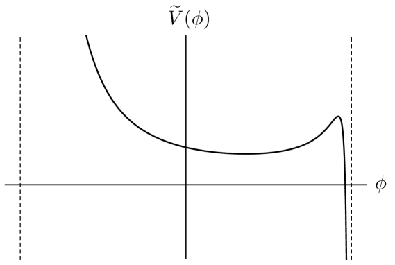
Figure 1: Effective potential for the $R\phi^{2}$ model.

To study stability we expand about the unstable point, $\phi=\langle\phi\rangle+\delta\phi$. To quadratic order the potential is (for $\rho_{\rm vac}^{\rm eff}\ll\rho_{\rm vac}$)

$$\widetilde{V}(\phi)=\rho_{\rm vac}^{\rm eff}-{\xi\rho_{\rm vac}\over(m_{P}^{\rm eff})^{2}}(\delta\phi)^{2}+{\cal O}((\delta\phi)^{3})\,.$$

The timescale associated with the instability is

$$\tau=\left(-\widetilde{V}^{\prime\prime}\right)^{-1/2}=\left({\rho_{\rm vac}^{\rm eff}\over 6\xi\rho_{\rm vac}}\right)^{1/2}H^{-1}\,.$$

So for sufficiently small $\xi$, say $\xi\lesssim 10^{-120}$, the solution will be stable for more than a Hubble time (and Hubble friction will play an important role in the evolution of $\phi$).

A.2 Solar system tests

In section 3 we constructed $F(R)$ models that give the right Planck length and de Sitter radius. However we also want models that are compatible with solar system tests of gravity. One way to achieve this is to give the scalar field a non-minimal kinetic term. As in (8) we take

$$S=\int d^{4}x\,\sqrt{-g}\left(f(\phi)R-{1\over 2}h(\phi)\partial_{\mu}\phi\partial^{\mu}\phi-V(\phi)\right)+S_{\rm matter}\,.$$

We assume that matter is minimally coupled to $g_{\mu\nu}$. By taking $h$ large any spatial variation in $\phi$ is suppressed and the model can be made compatible with solar system tests of gravity. Note that by a field redefinition $\phi\rightarrow\phi/\sqrt{\langle h\rangle}$ taking $h$ large is equivalent to making the scalar field very weakly coupled, i.e. $\xi$ small in the $R\phi^{2}$ context.

To show this in more detail we use the equivalence to Brans-Dicke gravity [26]. The classic solar system constraints on Brans-Dicke gravity were obtained by setting $V=0$. We can therefore translate the known constraints to our situation as long as terms related to $V$ in both the gravitational and scalar equations of motion are subdominant in the solar system. The Einstein equations read

$$G_{\mu\nu}=f^{-1}\left({1\over 2}T_{\mu\nu}^{\rm matter}+{1\over 2}T_{\mu\nu}^{\phi}+\nabla_{\mu}\nabla_{\nu}f-g_{\mu\nu}\Box f\right)$$ (46)

$$T_{\mu\nu}^{\phi}\equiv h\nabla_{\mu}\phi\nabla_{\nu}\phi-g_{\mu\nu}\left({1\over 2}h\nabla^{\rho}\phi\nabla_{\rho}\phi+V\right)$$

and the scalar equation of motion is

$$h\Box\phi+{1\over 2}{dh\over d\phi}\nabla^{\mu}\phi\nabla_{\mu}\phi-{dV\over d\phi}+{df\over d\phi}R=0\,.$$ (47)

¿From these equations it seems we need

$$fR\gg V\quad,\quad\left|{df\over d\phi}\right|R\gg\left|{dV\over d\phi}\right|$$ (48)

where $R$ is the curvature in the solar system. Recall that our static de Sitter solution has $f_{0}R_{0}=2V_{0}$ and $f^{\prime}_{0}R_{0}=V^{\prime}_{0}$, where $R_{0}\sim H_{0}^{2}\ll R_{\rm solar}$, and $f_{0}$ and $V_{0}$ denote cosmological vevs. It therefore seems the above two inequalities are easily satisfied. However there is an implicit assumption here, that the value of $\phi$ in the solar system does not differ too significantly from its cosmological value, so that $f_{\rm solar}\approx f_{0}$ and $V_{\rm solar}\approx V_{0}$. This will be true for sufficiently large $h$, as we now show.

To study the variation of $\phi$ within the solar system we linearize the scalar equation of motion, setting $\phi=\langle\phi\rangle+\delta\phi$ with $\delta\phi$ obeying

$$\nabla^{2}\delta\phi+{f_{0}^{\prime\prime}R-V_{0}^{\prime\prime}\over h_{0}}\delta\phi+{f_{0}^{\prime}(R-R_{0})\over h_{0}}=0\,.$$ (49)

For large $h_{0}$ we can neglect the mass term. The source term is dominated by the scalar curvature in the solar interior, where $R\approx\kappa_{\rm eff}^{2}\rho_{\odot}$. Thus to a good approximation

$$\nabla^{2}\delta\phi+{f_{0}^{\prime}\kappa_{\rm eff}^{2}M_{\odot}\over h_{0}}\delta^{3}({\bf x})=0\,.$$ (50)

So $\delta\phi$ is maximized at the surface of the sun, where

$$\delta\phi\approx{f_{0}^{\prime}\kappa_{\rm eff}^{2}M_{\odot}\over 4\pi h_{0}r_{\odot}}\,.$$ (51)

¿From (6) and (7) it follows that $\delta V/V\approx 2\,\delta\!f/f$, so we only need to impose

$${\delta V\over V}\approx{V_{0}^{\prime}f_{0}^{\prime}\kappa_{\rm eff}^{2}M_{\odot}\over 4\pi h_{0}V_{0}r_{\odot}}\ll 1\,.$$ (52)

This is easily satisfied for large $h_{0}$. Then the model is equivalent to Brans-Dicke theory, and solar system tests mostly bound two parameters [27]

$$\gamma={1+\omega\over 2+\omega}=1\pm O(10^{-5})\quad,\quad\beta=1+{\omega^{\prime}\over(3+2\omega)^{2}(4+2\omega)}=1\pm O(10^{-3})$$ (53)

where $\omega$ and $\omega^{\prime}$ are related to our $f$ and $h$ by:

$$\omega={1\over 2}hf\left({df\over d\phi}\right)^{-2}$$ (54)

$$\omega^{\prime}=2f\left({1\over 2}{dh\over d\phi}{f\over(df/d\phi)^{3}}+{1\over 2}{h\over(df/d\phi)^{2}}-{hf(d^{2}f/d\phi^{2})\over(df/d\phi)^{4}}\right)\,.$$ (55)

As long as $h$ is large enough the solar system tests are passed.

For example, as shown in [26], in the $R\phi^{2}$ model we have $h=1$, $f={1\over 2\kappa^{2}}-{1\over 2}\xi\phi^{2}$, $V=\rho_{\rm vac}-J\phi$ and therefore $\omega={1-\xi\kappa^{2}\phi^{2}\over 4\xi^{2}\kappa^{2}\phi^{2}}$. With the help of (26) this can be rewritten as

$$\omega={\rho_{\rm vac}^{\rm eff}\over\xi\left(\rho_{\rm vac}-\rho_{\rm vac}^{\rm eff}\right)}\,.$$ (56)

The bound (53) requires $\omega\gtrsim 10^{5}$ (we take $\omega>-3/2$ so that in Einstein frame the Brans-Dicke scalar has a right-sign kinetic term). This leads to the constraint on $\xi$ in (28). However for this constraint to be valid we should make sure that (52) is satisfied. Using $J\phi\approx\rho_{\rm vac}$ (52) can be rewritten as

$$\xi\ll 4\pi\cdot{\rho_{\rm vac}^{\rm eff}\over\rho_{\rm vac}}\cdot{r_{\odot}\over\kappa_{\rm eff}^{2}M_{\odot}}=4\pi\cdot 10^{-120}\cdot 10^{5}\,.$$ (57)

This is less stringent than (28).

A.3 Matter and radiation domination

The de Sitter solutions we found give us phenomenologically acceptable cosmic acceleration today. Here we study the conditions under which these solutions can be extended to the early universe in the presence of matter and radiation. More concretely we seek a solution of the form $\phi=\phi_{0}+\phi_{1}$ where $\phi_{0}$ is a constant chosen to give us phenomenologically acceptable cosmic acceleration today and $\phi_{1}$ is a small time-dependent perturbation. It is by no means obvious that this is the most interesting dynamical solution, but such a quasi-static solution for the scalar field, if it exists, provides a particularly simple way to satisfy all observational constraints.

Applying the FRW ansatz to the equations of motion of the $R\phi^{2}$ model we find

$$-R={2\over M_{b}^{2}-\xi\phi^{2}}\Big{[}{1\over 2}(-\rho+3p)^{\rm matter}+{1\over 2}(h\dot{\phi}^{2}-4(\rho_{\rm vac}+J\phi))$$ (58)

$$\quad\quad\quad-3(\xi\phi(\ddot{\phi}+3H\dot{\phi})+\xi\dot{\phi}^{2})\Big{]}$$

where we have taken the trace of the Einstein equations (46). The scalar equation of motion is

$$h(\ddot{\phi}+3H\dot{\phi})+{1\over 2}h^{\prime}\dot{\phi}^{2}=-J-\xi\phi R\,.$$ (59)

The static de Sitter solution obeys

$$J+\xi\phi_{0}R_{0}=0\,,\quad R_{0}=4(\rho_{\rm vac}+J\phi_{0})/(M_{b}^{2}-\xi\phi_{0}^{2})$$ (60)

where $R_{0}=12H_{0}^{2}$ is the curvature today and where we defined

$$\rho_{\rm vac}^{\rm eff}\equiv\rho_{\rm vac}+J\phi\,,\quad M_{\rm pl}^{2}\equiv M_{b}^{2}-\xi\phi_{0}^{2}\,.$$ (61)

Here $M_{b}$ is the bare Planck mass (the quantity we denoted $m_{P}$ previously).

Going back in time, the source term for the $\ddot{\phi}$ equation is $J+\xi\phi R\approx\xi\phi R$ because $R\propto a^{-3}$ during matter domination (we will discuss radiation domination below). Assuming $\phi_{1}\ll\phi_{0}$ we therefore have

$${H\over a^{2}}{d\over da}\left[a^{4}H{d\phi_{1}\over da}\right]\sim-3{\xi\over h}\phi_{0}H^{2}$$ (62)

where we have used $\ddot{\phi}_{1}+3H\dot{\phi}_{1}=(H/a^{2})(d/da)[a^{4}Hd\phi/da]$ and $R=3H^{2}$ during matter domination. Integrating we have

$$\phi_{1}=-3{\xi\over h}\phi_{0}\int{da\over a^{4}H}\left[\int a^{2}Hda\right]+A\int{da\over a^{4}H}+B$$ (63)

where $A$ and $B$ are dictated by initial conditions. The constant $B$ can be absorbed into $\phi_{0}$. The mode associated with $A$ decays with time, and one can reasonably argue that for a wide range of initial conditions this mode will be subdominant at all times relevant for observation. There remains the driven mode, given by

$$\phi_{1}=-2{\xi\over h}\phi_{0}\ {\rm ln}\ a\,.$$ (64)

Clearly one can make $\phi_{1}\ll\phi_{0}$ by choosing $\xi/h\ll 1$. The weak dependence on $a$ means it is easy to satisfy $\phi_{1}\ll\phi_{0}$ for all observationally relevant scale factors. However to be self-consistent we also need to check that the perturbation does not dominate over the matter energy density and pressure in (58). Examining the various contributions from $\phi_{1}$ and its derivatives, the dominant contributions are of order $(\xi^{2}/h)H^{2}\phi_{0}^{2}$ (such as from $\dot{\phi}_{1}^{2}$), and the self-consistency requirement is that this is much smaller than $\rho^{\rm matter}\sim H^{2}M_{\rm pl}^{2}$. In other words, we need to make sure that $(\xi/h)\xi\phi_{0}^{2}\ll M_{\rm pl}^{2}$. Recall that the phenomenologically interesting static de Sitter solution has $M_{b}^{2}\gg M_{\rm pl}^{2}$, which basically means $\xi\phi_{0}^{2}\sim M_{b}^{2}$ (see (61)). Therefore a solution for the scalar field that does not significantly modify the expansion rate at early times requires

$${\xi\over h}\ll{M_{\rm pl}^{2}\over M_{b}^{2}}\sim{\rho_{\rm vac}^{\rm eff}\over\rho_{\rm vac}}\,.$$ (65)

This requirement is rather severe, but it happens to be about the same as the requirement for stability of the static solution.

What happens if we go back even further, to the era of radiation domination? An interesting observation is that due to its traceless stress tensor radiation makes no contribution to $R$. However this doesn’t mean $R$ vanishes, due to the stress tensor for $\phi$, so in fact a quasi-static scalar field would mean $R\sim R_{0}+\delta R$ during radiation domination. Then the $\phi$ equation of motion (59) tells us

$$\ddot{\phi}_{1}+3H\dot{\phi}_{1}=-{\xi\over h}R_{0}\phi_{1}-{\xi\over h}\phi_{0}\delta R$$

$$\quad\quad\quad\quad=-{\xi\over h}R_{0}\phi_{1}+2{\xi\over h}R_{0}\phi_{1}{\xi\phi_{0}^{2}\over M_{\rm pl}^{2}}-6{\xi\over h}{\xi\phi_{0}^{2}\over M_{\rm pl}^{2}}(\ddot{\phi}_{1}+3H\dot{\phi}_{1})$$

$$\quad\quad\quad\quad\approx 2{\xi\over h}{M_{b}^{2}\over M_{\rm pl}^{2}}R_{0}\phi_{1}-6{\xi\over h}{M_{b}^{2}\over M_{\rm pl}^{2}}(\ddot{\phi}_{1}+3H\dot{\phi}_{1})$$ (66)

where we’ve used the fact that $J+\xi\phi_{0}R_{0}=0$.

We’re allowing $\phi_{1}$ to evolve on cosmological time-scales, so $H\dot{\phi}_{1}\sim H^{2}\phi_{1}$ which is much larger than $(\xi/h)(M_{b}^{2}/M_{\rm pl}^{2})R_{0}\phi_{1}$. This means we can drop the first term on the right hand side of (66). Also given (65) we can drop the last term on the right hand side of (66). So we’re left with a very simple equation

$$\ddot{\phi}_{1}+3H\dot{\phi}_{1}\sim 0$$ (67)

with solution

$$\phi_{1}=A/a+B\,.$$ (68)

$A$ and $B$ are determined by initial conditions. $B$ can be absorbed into $\phi_{0}$, and $A$ can always be chosen to be small enough to satisfy any self-consistency requirements one needs to impose. (Think of it this way: suppose $A/a$ takes some natural value in the very early universe, then for the $a$’s of interest it is likely that $A/a$ is very small.) The upshot is that a quasi-static approximation for the scalar field is valid during radiation domination as well.

In summary, the presence of matter and radiation is consistent with a quasi-static scalar field as long as (65) is satisfied. A similar analysis with similar conclusions can be made for the Gauss-Bonnet model.

A.4 Radiative stability

So far we have treated the $F(R)$ models as classical field theories. But one of the central mysteries of the cosmological constant is whether it can be protected from large radiative corrections. In this section we study quantum effects. To be concrete we will focus on the $R\phi^{2}$ model, although similar results should hold in general $F(R)$ models.

First let’s consider the model in Jordan frame.

$$S=\int d^{4}x\sqrt{-g}\left({1\over 2\kappa^{2}}R-{1\over 2}(\partial\phi)^{2}-{1\over 2}\xi R\phi^{2}+J\phi-\rho_{\rm vac}\right)$$

A key observation is that $\xi=J=0$ is an enhanced symmetry point, where the theory is invariant under shifts $\phi\rightarrow\phi+{\rm const}$. This means radiative corrections to quantities like $\xi$, $J$ and the scalar mass $m$ (set to zero above) have to be proportional to the symmetry-breaking parameters $\xi$ and $J$ themselves. To summarize the results of our analysis: radiative corrections to these symmetry-breaking parameters are under control if $\xi$ is sufficiently small, roughly $|\xi|<10^{-120}$. However this argument does not address radiative corrections to the vacuum energy $\rho_{\rm vac}$ itself. Indeed we will find that, from the point of view of quantum corrections to $\rho_{\rm vac}$, the $R\phi^{2}$ model is just as unstable as a bare cosmological constant.

We will perform the rest of our analysis in Einstein frame.

$$S=\int d^{4}x\sqrt{-\widetilde{g}}\left({1\over 2(\kappa_{\rm eff})^{2}}\widetilde{R}-{1\over 2}\widetilde{h}(\phi)\widetilde{g}^{\mu\nu}\partial_{\mu}\phi\partial_{\nu}\phi-\widetilde{V}(\phi)\right)$$

We will concentrate on quantum corrections to the scalar potential $\widetilde{V}$. Before studying our model, consider a scalar field theory in flat space with a potential

$$V_{\rm flat}=\rho+J\phi+{1\over 2}m^{2}\phi^{2}+{1\over 3}g\phi^{3}+{1\over 4}\lambda\phi^{4}\,.$$

In this flat-space theory a one-loop vacuum bubble should make a correction

$$\raisebox{-17.07182pt}{\includegraphics[height=42.67912pt]{5.pdf}}\quad\Rightarrow\quad\Delta\rho\sim\Lambda_{UV}^{4}$$

where $\Lambda_{UV}$ is a UV cutoff scale. A one-loop wart diagram should make a correction to the scalar mass

$$\raisebox{-17.07182pt}{\includegraphics[height=42.67912pt]{6.pdf}}\quad\Rightarrow\quad\Delta m^{2}\sim\lambda\Lambda_{UV}^{2}\,.$$

Finally a one-loop tadpole diagram should make a correction to the source

$$\raisebox{-17.07182pt}{\includegraphics[height=42.67912pt]{7.pdf}}\quad\Rightarrow\quad\Delta J\sim g\Lambda_{UV}^{2}\,.$$

This will generate a shift in the vev

$$\Delta\langle\phi\rangle=-\Delta J/m^{2}$$

which in turn produces a shift in the vacuum energy (for $J=0$)

$$\Delta\langle V\rangle=(\Delta J)^{2}/2m^{2}\,.$$

What do these results mean for the $R\phi^{2}$ model? Setting $\phi=\langle\phi\rangle+\delta\phi$, the effective potential of the $R\phi^{2}$ model has an expansion in powers of $J\delta\phi/\rho_{\rm vac}^{\rm eff}$.

$$\widetilde{V}(\phi) = {\kappa^{4}\over(\kappa_{\rm eff})^{4}}{\rho_{\rm vac}-J\phi\over(1-\xi\kappa^{2}\phi^{2})^{2}}$$

$$= \rho_{\rm vac}^{\rm eff}-{J^{2}\over 4\rho_{\rm vac}^{\rm eff}}(\delta\phi)^{2}-{J^{3}\over 4(\rho_{\rm vac}^{\rm eff})^{2}}(\delta\phi)^{3}-{3J^{4}\over 16(\rho_{\rm vac}^{\rm eff})^{3}}(\delta\phi)^{4}+{\cal O}(\delta\phi^{5})$$

There are three classes of corrections we will study.

Corrections to $m_{\phi}^{2}$

In Einstein frame the scalar mass is

$$m_{\rm Einstein}^{2}\sim J^{2}/\rho_{\rm vac}^{\rm eff}\,.$$

Given the quartic coupling in our model the radiative correction gives

$$\Delta m_{\rm Einstein}^{2}\sim J^{4}\Lambda_{UV}^{2}/(\rho_{\rm vac}^{\rm eff})^{3}$$

or

$${\Delta m_{\rm Einstein}^{2}\over m_{\rm Einstein}^{2}}\sim{J^{2}\Lambda_{UV}^{2}\over(\rho_{\rm vac}^{\rm eff})^{2}}\sim{\xi\rho_{\rm vac}\over\rho_{\rm vac}^{\rm eff}}\cdot{\Lambda_{UV}^{2}\over(m_{P}^{\rm eff})^{2}}\,.$$

Radiative corrections to the scalar mass are stabilized for $\xi\lesssim 10^{-120}$, assuming $\rho_{\rm vac}\sim(m_{P}^{\rm eff})^{4}$ and $\Lambda_{UV}\sim m_{P}^{\rm eff}$.

Linear source term

In Einstein frame we’ll generate a linear source term for the scalar field

$$\Delta J\sim J^{3}\Lambda_{UV}^{2}/(\rho_{\rm vac}^{\rm eff})^{2}\,.$$

This shifts the vev and in turn corrects the vacuum energy.

$$\Delta\widetilde{V}\sim(\Delta J)^{2}/m_{\rm Einstein}^{2}\sim J^{4}\Lambda_{UV}^{4}/(\rho_{\rm vac}^{\rm eff})^{3}$$

The quantity we need to look at is

$${\Delta\widetilde{V}\over\rho_{\rm vac}^{\rm eff}}\sim{J^{4}\Lambda_{UV}^{4}\over(\rho_{\rm vac}^{\rm eff})^{4}}\sim\left({\xi\rho_{\rm vac}\over\rho_{\rm vac}^{\rm eff}}\right)^{2}{\Lambda_{UV}^{4}\over(m_{P}^{\rm eff})^{4}}\,.$$

Again radiative corrections are stabilized for $\xi\lesssim 10^{-120}$, assuming $\rho_{\rm vac}\sim(m_{P}^{\rm eff})^{4}$ and $\Lambda_{UV}\sim m_{P}^{\rm eff}$.

Corrections to $\rho_{\rm vac}^{\rm eff}$

Here the $R\phi^{2}$ model suffers from the usual instability of vacuum energy with respect to radiative corrections: in Einstein frame, no symmetry forbids graviton loops or $\phi$ loops from generating

$$\Delta\rho_{\rm vac}^{\rm eff}\sim\Lambda_{UV}^{4}\,.$$

This means the $R\phi^{2}$ model doesn’t avoid the usual naturalness problems associated with vacuum energy. Although this is easiest to see in Einstein frame, one can reach the same conclusion in Jordan frame. In Jordan frame graviton and $\phi$ loops, or loops of standard model particle fields, should generate a shift $\Delta\rho_{\rm vac}\sim\Lambda_{UV}^{4}$. This change in $\rho_{\rm vac}$ can be compensated by shifting $\langle\phi\rangle$ to preserve a small $\rho_{\rm vac}^{\rm eff}$, but the necessary change in $\langle\phi\rangle$ completely destabilizes the effective Planck mass. To be more explicit about the difficulty, suppose we have a correction in Jordan frame

$$\Delta\rho_{\rm vac}\sim\Lambda_{UV}^{4}\,.$$

You might think we’ve achieved something: with $\rho_{\rm vac}\sim(m_{P}^{\rm eff})^{4}$ and $\Lambda_{UV}\sim m_{P}^{\rm eff}$, don’t we naturally have $\Delta\rho_{\rm vac}/\rho_{\rm vac}={\cal O}(1)$? Unfortunately the relation (30)

$${J^{2}m_{P}^{2}\over\xi\rho_{\rm vac}^{2}}=1+10^{-120}$$

requires $\Delta\rho_{\rm vac}/\rho_{\rm vac}\lesssim 10^{-120}$. Equivalently, it requires $\Delta\rho_{\rm vac}\lesssim\rho_{\rm vac}^{\rm eff}$. So the $R\phi^{2}$ model is just as sensitive to radiative corrections as a pure cosmological constant.

To summarize, with $\xi\lesssim 10^{-120}$ radiative corrections to the non-constant parts of the scalar potential seem to be under control. It’s curious that this value of $\xi$ was already required for cosmological stability. However the constant term in the potential is not protected, and makes the $R\phi^{2}$ model just as unstable with respect to quantum corrections as a bare cosmological constant. We expect this last conclusion to apply to any $F(R)$ model, since any $F(R)$ model can be given a scalar-tensor description and mapped to Einstein frame as in (44).

Appendix B Further examples of $F(R)$

In this appendix we present further examples of modified gravity actions, built purely from the scalar curvature, which have low-curvature de Sitter solutions. As in section 3 we will write the action as

$$S=\int d^{4}x\,\sqrt{-g}\,(m_{P}^{\rm eff})^{4}F(y)$$

where

$$y=R/4(m_{P}^{\rm eff})^{2}\,.$$

Recall that any function $F(y)$ satisfying (16), namely

$$F(\epsilon)=\epsilon\qquad\quad F^{\prime}(\epsilon)=2\,,$$ (70)

will have a low-curvature de Sitter solution with the right effective Planck mass, where $\epsilon=3H_{0}^{2}/(m_{P}^{\rm eff})^{2}\sim 10^{-120}$.

Clearly an infinite number of functions satisfy (70): $F(y)={\rm exp}\,(y^{2}/\epsilon)-1$, $\,\,\sqrt{1+2y^{2}/\epsilon}-1$, $\,\,2\epsilon\log(y/\epsilon)+\epsilon$, $\,\ldots$  To be a bit more systematic about this we make the ansatz

$$F(y)=\sum_{n=-\infty}^{\infty}a_{n}y^{n}\,.$$ (71)

Then (70) implies the conditions

$$\sum_{n}a_{n}\epsilon^{n}=\epsilon,\qquad\sum_{n}na_{n}\epsilon^{n-1}=2\,.$$ (72)

Here are a few examples.

Example 1. We can satisfy the necessary conditions with a single coupling constant by taking $F(y)=y^{2}/\epsilon$. That is, the gravity action

$$S=\int d^{4}x\,\sqrt{-g}\,R^{2}/16\epsilon$$ (73)

has a solution with both the correct Planck mass and the correct vacuum energy. To make the model compatible with solar tests we invert the Legendre transform and add a large scalar kinetic term.

$$S=\int d^{4}x\,\sqrt{-g}\,\left(\phi R-{1\over 2}h(\partial\phi)^{2}-4\epsilon\phi^{2}\right)$$ (74)

One curious feature: neglecting the scalar kinetic term, this action is invariant under the scale transformation

$$g_{\mu\nu}\rightarrow ag_{\mu\nu}\qquad\phi\rightarrow\phi/a\,.$$ (75)

This means the model has de Sitter solutions with arbitrary radius (and varying Planck mass). It is an extreme example of the fact that, although (70) guarantees the existence of a solution with the desired properties, it does not preclude other de Sitter solutions.

Example 2. With two coupling constants, the most obvious way to satisfy (70) is to take $F(y)=2y-\epsilon$. This just corresponds to ordinary Einstein gravity with a small cosmological constant. Another option is to choose $F=-2\epsilon^{2}/y+3\epsilon$. Going to the scalar-tensor description, and adding a large scalar kinetic term, the latter example shows that an Einstein-Hilbert term is not necessary to pass solar system tests.

The examples we have considered so far do not interest us much, because we want models with $a_{0}\sim-1$ representing a Planck-scale bare vacuum energy. Our remaining examples have arbitrary $a_{0}$.

Example 3. Choose

$$a_{0}={\rm arbitrary}\quad,\quad a_{1}={3\epsilon-a_{0}\over 2\epsilon}\quad,\quad a_{-1}=-\epsilon(a_{0}+\epsilon)/2$$ (76)

and the rest of the $a_{n}$’s vanish. That is, the gravitational action is

$$S=(m_{P}^{\rm eff})^{4}\int d^{4}x\sqrt{-g}\left({a_{1}R\over 4(m_{P}^{\rm eff})^{2}}+{4(m_{P}^{\rm eff})^{2}a_{-1}\over R}+a_{0}\right)\,.$$ (77)

Inverting the Legendre transformation, and choosing the relation between $f$ and $\phi$ to set $\phi=(m_{P}^{\rm eff})^{3}/R$, this is equivalent to the $R\phi^{2}$ model studied in section 4. The scalar-tensor action is

$$S=\int d^{4}x\sqrt{-g}\left[\Big{(}{a_{1}(m_{P}^{\rm eff})^{2}\over 4}-4a_{-1}\phi^{2}\Big{)}R-{1\over 2}h(\partial\phi)^{2}-V(\phi)\right]$$

$$V(\phi)=-8(m_{P}^{\rm eff})^{3}a_{-1}\phi-(m_{P}^{\rm eff})^{4}a_{0}$$ (78)

where we added a kinetic term for $\phi$.

Example 4. Choose

$$a_{0}={\rm arbitrary}\quad,\quad a_{-1}=-2\epsilon(a_{0}-2\epsilon)\quad,\quad a_{-2}=\epsilon^{2}(a_{0}-3\epsilon)$$ (79)

and the rest of the $a_{n}$’s vanish. That is, the gravitational action is

$$S=(m_{P}^{\rm eff})^{4}\int d^{4}x\sqrt{-g}\left({4(m_{P}^{\rm eff})^{2}a_{-1}\over R}+{16(m_{P}^{\rm eff})^{4}a_{-2}\over R^{2}}+a_{0}\right)\,.$$ (80)

This looks strange, but remember that for solar system tests one must revert back to the scalar-tensor theory. Inverting the Legendre transform, and again taking $\phi=(m_{P}^{\rm eff})^{3}/R$, we have the equivalent scalar-tensor theory

$$S=\int d^{4}x\sqrt{-g}\left[\Big{(}-4a_{-1}\phi^{2}-{32a_{-2}\phi^{3}\over m_{P}^{\rm eff}}\Big{)}R-{1\over 2}h(\partial\phi)^{2}-V(\phi)\right]$$

$$V(\phi)=-8(m_{P}^{\rm eff})^{3}a_{-1}\phi-48(m_{P}^{\rm eff})^{2}a_{-2}\phi^{2}-(m_{P}^{\rm eff})^{4}a_{0}\,.$$ (81)

Appendix C More on Gauss-Bonnet

In this appendix we study the classical stability of solutions to the Gauss-Bonnet equations of motion, and show that for $\xi\lesssim 1$ the low-curvature de Sitter solution is metastable for more than a Hubble time.

C.1 Equations of motion

We consider a generalized Gauss-Bonnet action coupled to matter,

$$S=\int d^{4}x\sqrt{-g}\left[\frac{1}{2\kappa^{2}}R-\frac{1}{2}h(\phi)\partial_{\mu}\phi\partial^{\mu}\phi-V(\phi)-f(\phi){\cal G}\right]+S_{M}$$ (82)

where the Euler density is

$${\cal G}=R^{2}-4R^{\mu\nu}R_{\mu\nu}+R^{\mu\nu\kappa\lambda}R_{\mu\nu\kappa\lambda}\,.$$ (83)

Define the following tensor

$${\cal G}^{\mu\nu} \equiv {1\over\sqrt{-g}}{\delta\over\delta g_{\mu\nu}}\left[\sqrt{-g}f(\phi){\cal G}\right]$$

$$= 2R\nabla^{\mu}\nabla^{\nu}f(\phi)+2g^{\mu\nu}\left[2R_{\rho\sigma}\nabla^{\rho}\nabla^{\sigma}f(\phi)-R\Box f(\phi)\right]$$

$$-8R^{\rho(\mu}\nabla^{\nu)}\nabla_{\rho}f(\phi)+4R^{\mu\nu}\Box f(\phi)-4R^{\mu\rho\nu\sigma}\nabla_{\rho}\nabla_{\sigma}f(\phi).$$

The equations of motion for the metric are then

$$R_{\mu\nu}-\frac{1}{2}Rg_{\mu\nu}=\kappa^{2}\Big{[}T^{M}_{\mu\nu}+T_{\mu\nu}^{\phi}-2{\cal G}_{\mu\nu}\Big{]}$$ (85)

where

$$T_{\mu\nu}^{\phi}=h(\phi)\left(\partial_{\mu}\phi\partial_{\nu}\phi-\frac{1}{2}g_{\mu\nu}(\partial\phi)^{2}\right)-g_{\mu\nu}V(\phi)\,.$$ (86)

The equation of motion for the scalar field is

$$h(\phi)\Box\phi+{1\over 2}h^{\prime}(\phi)\partial^{\mu}\phi\partial_{\mu}\phi-V^{\prime}(\phi)-f^{\prime}(\phi){\cal G}=0\,.$$ (87)

It’s a remarkable property of Gauss-Bonnet gravity that one obtains second-order equations of motion, even though one is starting from a higher-derivative action which naively would be expected to generate fourth-order equations [20].

In maximally symmetric spacetimes we have

$$R_{\mu\nu}-\frac{1}{2}Rg_{\mu\nu}=-{1\over 4}Rg_{\mu\nu}$$

$${\cal G}={R^{2}/6}$$

$${\cal G}_{\mu\nu}=0\,.$$

In the absence of matter, and assuming a maximally symmetric metric and constant $\phi$, the equations of motion simplify to

$$R=4\kappa^{2}V(\phi)$$

$$V^{\prime}(\phi)=-\frac{1}{6}f^{\prime}(\phi)R^{2}\,.$$ (88)

These are the Gauss-Bonnet analogs of (6), (7) in $F(R)$ gravity. We see that critical points of the scalar potential are not what give us de Sitter solutions. Rather we must look for points on the potential such that

$$V^{\prime}(\phi)=-\frac{8}{3}\kappa^{4}f^{\prime}(\phi)V(\phi)^{2}\,.$$ (89)

C.2 Classical stability

Here we show that for $\xi\lesssim 1$ the low-curvature de Sitter solution is metastable on cosmological timescales. Plugging in the FRW ansatz

$$ds^{2}=-dt^{2}+a^{2}(t)|d\vec{x}|^{2}\ ,\ \ \ \phi=\phi(t)$$ (90)

we obtain the Friedmann equation from the $\mu\nu=00$ component of (85),

$$\frac{3}{\kappa^{2}}H^{2}-\frac{h}{2}{\dot{\phi}}^{2}-V(\phi)-24\dot{\phi}f^{\prime}(\phi)H^{3}=\rho_{M}$$ (91)

where $\rho_{M}$ is the matter energy density. Assuming constant $h$, the scalar equation of motion (87) becomes

$$h\left(\ddot{\phi}+3H\dot{\phi}\right)+V^{\prime}(\phi)+24f^{\prime}(\phi)H^{2}\left(\dot{H}+H^{2}\right)=0\ .$$ (92)

In these equations $H\equiv\dot{a}/a$ is the Hubble parameter and some useful identities are

$$R=6\dot{H}+12H^{2},\ \ \ {\cal G}=24H^{2}(\dot{H}+H^{2})\,.$$ (93)

The remaining components of (85) do not yield independent equations, but rather are consequences of (91) and (92).

We are interested in fluctuations about a low curvature de Sitter solution in which $H$ and $\phi$ are constant. Setting

$$H(t)=H_{0}+\delta H(t),\ \ \ \phi(t)=\phi_{0}+\delta\phi(t)$$ (94)

to first order in the fluctuations (91) reads (in the absence of matter)

$$24f^{\prime}H_{0}^{3}\delta\dot{\phi}+V^{\prime}\delta\phi-{6H_{0}\over\kappa^{2}}\delta H=0$$ (95)

where $f^{\prime}$ and $V^{\prime}$ are evaluated on $\phi_{0}$. Similarly (92) reads

$$h\delta\ddot{\phi}+3hH_{0}\delta\dot{\phi}+\left(V^{\prime\prime}+24f^{\prime\prime}H_{0}^{4}\right)\delta\phi+24f^{\prime}H_{0}^{2}\delta\dot{H}+96f^{\prime}H_{0}^{3}\delta H=0\,.$$ (96)

Solving (95) for $\delta H$ and plugging into (96) gives an equation for $\delta\phi$,

$$\delta\ddot{\phi}+3H_{0}\delta\dot{\phi}+\frac{V^{\prime\prime}-384\kappa^{2}f^{\prime 2}H_{0}^{6}+24f^{\prime\prime}H_{0}^{4}}{h+96\kappa^{2}f^{\prime 2}H_{0}^{4}}\delta\phi=0$$ (97)

where we used (88) to eliminate $V^{\prime}$. Specializing to our model we set

$$V(\phi)=\rho_{\rm vac}-J\phi\,,\qquad f(\phi)={1\over 2}\xi\kappa^{2}\phi^{2}\,.$$ (98)

Then (97) reduces to (for $\rho_{\rm vac}\gg\rho_{\rm vac}^{\rm eff}$, and using (36) to eliminate the vev)

$$\delta\ddot{\phi}+3H_{0}\delta\dot{\phi}-16{\xi\over h}H_{0}^{2}\left({\kappa^{4}\rho_{\rm vac}\over 1+4(\xi/h)\kappa^{4}\rho_{\rm vac}}\right)\delta\phi=0\,.$$ (99)

This means the low-curvature de Sitter solution is unstable. Assuming $\rho_{\rm vac}\sim m_{P}^{4}$ and $\xi/h\lesssim 1$ the factor in parenthesis is ${\cal O}(1)$. So the timescale for the instability is

$$\tau\sim\left({h\over\xi}\right)^{1/2}H_{0}^{-1}\,.$$ (100)

Provided $\xi/h\lesssim 1$ the solution will be metastable for more than a Hubble time, and Hubble friction will play an important role in the evolution of $\phi$.

References

• [1] S. Weinberg, “The cosmological constant problem,” Rev. Mod. Phys. 61 (1989) 1–23.
• [2] S. Weinberg, “Theories of the cosmological constant,” astro-ph/9610044.
• [3] S. M. Carroll, “The cosmological constant,” Living Rev. Rel. 4 (2001) 1, astro-ph/0004075.
• [4] S. Weinberg, “The cosmological constant problems,” astro-ph/0005265.
• [5] J. Polchinski, “The cosmological constant and the string landscape,” hep-th/0603249.
• [6] S. Nobbenhuis, “Categorizing different approaches to the cosmological constant problem,” Found. Phys. 36 (2006) 613–680, gr-qc/0411093.
• [7] R. Bousso and J. Polchinski, “Quantization of four-form fluxes and dynamical neutralization of the cosmological constant,” JHEP 06 (2000) 006, hep-th/0004134.
• [8] M. R. Douglas and S. Kachru, “Flux compactification,” Rev. Mod. Phys. 79 (2007) 733–796, hep-th/0610102.
• [9] S. M. Carroll, V. Duvvuri, M. Trodden, and M. S. Turner, “Is cosmic speed-up due to new gravitational physics?,” Phys. Rev. D70 (2004) 043528, astro-ph/0306438.
• [10] S. Weinberg, The Quantum theory of fields. Vol. 1: Foundations. Cambridge Univ. Press, 1995. See section 7.7.
• [11] S. Nojiri and S. D. Odintsov, “Introduction to modified gravity and gravitational alternative for dark energy,” eConf C0602061, 06 (2006) [Int. J. Geom. Meth. Mod. Phys.  4, 115 (2007)] [arXiv:hep-th/0601213].
• [12] R. P. Woodard, “Avoiding dark energy with 1/R modifications of gravity,” Lect. Notes Phys.  720, 403 (2007) [arXiv:astro-ph/0601672].
• [13] S. Nojiri and S. D. Odintsov, “Modified gravity with negative and positive powers of the curvature: Unification of the inflation and of the cosmic acceleration,” Phys. Rev.  D 68, 123512 (2003) [arXiv:hep-th/0307288].
• [14] T. Chiba, “1/R gravity and scalar-tensor gravity,” Phys. Lett. B575 (2003) 1–3, astro-ph/0307338.
• [15] W. Hu and I. Sawicki, “Models of f(R) cosmic acceleration that evade solar-system tests,” Phys. Rev. D76 (2007) 064004, arXiv:0705.1158 [astro-ph].
• [16] B. Boisseau, G. Esposito-Farese, D. Polarski and A. A. Starobinsky, “Reconstruction of a scalar-tensor theory of gravity in an accelerating universe,” Phys. Rev. Lett.  85, 2236 (2000) [arXiv:gr-qc/0001066].
• [17] T. Chiba, T. L. Smith, and A. L. Erickcek, “Solar System constraints to general f(R) gravity,” Phys. Rev. D75 (2007) 124014, astro-ph/0611867.
• [18] S. M. Carroll et al., “The cosmology of generalized modified gravity models,” Phys. Rev. D71 (2005) 063513, astro-ph/0410031.
• [19] I. P. Neupane, “Constraints on Gauss-Bonnet Cosmologies,” arXiv:0711.3234 [hep-th].
• [20] K. S. Stelle, “Classical gravity with higher derivatives,” Gen. Rel. Grav. 9 (1978) 353–371.
• [21] B. Zwiebach, “Curvature Squared Terms and String Theories,” Phys. Lett. B156 (1985) 315.
• [22] L. Amendola, C. Charmousis, and S. C. Davis, “Solar System Constraints on Gauss-Bonnet Mediated Dark Energy,” arXiv:0704.0175 [astro-ph].
• [23] A. Linde, “Inflation and quantum cosmology,”. In Three hundred years of gravitation, eds. S.W. Hawking and W. Israel. Cambridge University Press (1987). See p. 622.
• [24] J. Garriga, A. Linde, and A. Vilenkin, “Dark energy equation of state and anthropic selection,” Phys. Rev. D69 (2004) 063521, hep-th/0310034.
• [25] L. McAllister and E. Silverstein, “String Cosmology: A Review,” arXiv:0710.2951 [hep-th]. See section 3.2.3.
• [26] T. Chiba, “Quintessence, the gravitational constant, and gravity,” Phys. Rev. D60 (1999) 083508, gr-qc/9903094.
• [27] C. M. Will, “The confrontation between general relativity and experiment,” gr-qc/0510072.